Invariant Solutions and Conservation Laws of the Variable-Coefficient Heisenberg Ferromagnetic Spin Chain Equation

The variable-coefficient Heisenberg ferromagnetic spin chain (vcHFSC) equation is investigated using the Lie group method. The infinitesimal generators and Lie point symmetries are reported. Four types of similarity reductions are acquired by virtue of the optimal system of one-dimensional subalgebras. Several invariant solutions are derived, including trigonometric and hyperbolic function solutions. Furthermore, conservation laws for the vcHFSC equation are obtained with the help of Lagrangian and non-linear self-adjointness.

Introduction

The investigation of physical phenomenon modeled by non-linear partial differential equations (NLPDEs) and searching for their underlying dynamics remain the hot issue of research for applied and theoretical sciences. A lot of attention has been concentrated on looking for the explicit solutions of NLPDEs, for they can provide accurate information with which to understand some interesting physical phenomena. A great many powerful methods have been proposed to construct the explicit solutions of NLPDEs, such as the inverse scattering method [1], the Lie group method [2–5], the Hirota bilinear method [6, 7], the extended tanh method [8–10], the homoclinc test method [11–13], the F-expansion technique [14], and so on [15–18]. Among these methods, the Lie group method is a powerful and prolific method for the study of NLPDEs. On the one hand, based on the Lie group method, we can obtain new exact solutions directly or from the known ones or via similarity reductions; on the other hand, the conservation laws can be constructed via the corresponding Lie point symmetries. Recently, invariant solutions of a class of constant and variable coefficient NLPDEs have been obtained by virtue of this method, such as Keller-Segel models [19], generalized fifth-order non-linear integrable equation [20], KdV equation [21], and Davey-Stewartson equation [22].

So far, many effective methods have been extended to construct exact solutions of different types of differential equations. For example, the generalized Bernoulli sub-ODE and the generalized tanh methods have been applied to establish optical soliton solutions of the Chen-Lee-Liu equation [23]. The Lie group method has been used to find the exact solutions of the time fractional Abrahams–Tsuneto reaction diffusion system [24] and the non-linear transmission line equation [25].

In this work, we will focus on the (2+1)-dimensional variable-coefficient Heisenberg ferromagnetic spin chain (vcHFSC) equation

$\begin{array}{ll}i{q}_t+{\delta }_1(t)q_{xx}+{\delta }_2(t)q_{yy}+{\delta }_3(t)q_{xy}+{\delta }_4(t){\left|q\right|}^{2}q=0,& (1)\end{array}$

where δ₁(t), δ₂(t), δ₃(t), and δ₄(t) are arbitrary functions with respect to t. The interaction properties and stability of the bright and dark solitons are presented in [26]. Non-autonomous complex wave and analytic solutions are obtained in [27]. When δ_i(t) (i = 1, ⋯ , 4) are arbitrary constants, Equation (1) can be reduced to the following (2+1)-dimensional Heisenberg ferromagnetic spin chain (HFSC) equation:

$\begin{array}{ll}i{q}_t+{\delta }_1{q}_{xx}+{\delta }_2{q}_{yy}+{\delta }_3{q}_{xy}+{\delta }_4{\left|q\right|}^{2}q=0.& (2)\end{array}$

Latha and Vasanthi [28] obtained multisoliton solutions by employing Darboux transformation and analyzed the interaction properties of Equation (2). Anitha et al. [29] derived the dynamical equations of motion by employing long wavelength approximation and discussed the complete non-linear excitation with the aid of sine-cosine function method. Periodic solutions were obtained by Triki and Wazwaz [30], and they also discussed conditions for the existence and uniqueness of wave solutions. Tang et al. [31] reported the explicit power series solutions and bright and dark soliton solutions of Equation (2), and they also obtained some other exact solutions via the sub-ODE method.

However, the Lie symmetries, invariant solutions, and conservation laws of the (2+1)-dimensional vcHFSC equation (1) have not been studied. In the current work, we study the vcHFSC equation (1) via the Lie group method and obtain new invariant solutions, including the trigonometric and hyperbolic function solutions. Moreover, based on non-linear self-adjointness, conservation laws for vcHFSC equation (1) are constructed.

The main structure of this paper is as follows. In section Lie Symmetry Analysis and Optimal System, based on the Lie symmetry analysis, we construct the Lie point symmetries and the optimal system of one-dimensional subalgebras for Equation (1). In section Symmetry Reductions and Invariant Solutions, four types of similarity reductions and some invariant solutions are studied by virtue of the optimal system. In section Non-linear Self-Adjointness and Conservation Laws, conservation laws for Equation (1) are obtained with the help of Lagrangian and non-linear self-adjointness. Section Results and Discussion provides the results and discussion. Finally, the conclusion is given in section Conclusion.

Lie Symmetry Analysis and Optimal System

In this section, our aim is to obtain the Lie point symmetries and the optimal system of the vcHFSC equation (1) by employing the Lie group method.

The vcHFSC equation (1) can be changed to the following system

$\begin{array}{ll}\{\begin{array}{l}{F}_1=u_t+{\delta }_1(t)v_{xx}+{\delta }_2(t)v_{yy}+{\delta }_3(t)v_{xy}\\ +{\delta }_4(t)(u^{2}v+v^3)=0,\\ F_2=-v_t+{\delta }_1(t)u_{xx}+{\delta }_2(t)u_{yy}+{\delta }_3(t)u_{xy}\\ +{\delta }_4(t)(u^3+u{v}^2)=0,\end{array}& (3)\end{array}$

by using the transformation

$\begin{array}{ll}q(x,y,t)=u(x,y,t)+iv(x,y,t),& (4)\end{array}$

where u(x, y, t) and v(x, y, t) are real and smooth functions.

Suppose that the associated vector field of system (3) is as follows:

$\begin{array}{l}V={\xi }^1(x,y,t,u,v)\frac{\partial }{\partial x}+{\xi }^2(x,y,t,u,v)\frac{\partial }{\partial y}+{\xi }^3(x,y,t,u,v)\frac{\partial }{\partial t}\\ +{\eta }^1(x,y,t,u,v)\frac{\partial }{\partial u}+{\eta }^2(x,y,t,u,v)\frac{\partial }{\partial v},& (5)\end{array}$

where ξ¹(x, y, t, u, v), ξ²(x, y, t, u, v), ξ³(x, y, t, u, v), η¹(x, y, t, u, v) and η²(x, y, t, u, v) are unknown functions that need to be determined.

If vector field (5) generates a symmetry of system (3), then V must satisfy symmetry condition

$\begin{array}{ll}p{r}^{(2)}V({\Delta }_1){|}_{{\Delta }_1}=0,p{r}^{(2)}V({\Delta }_2){|}_{{\Delta }_2}=0,& (6)\end{array}$

where

$\begin{array}{l}\{\begin{array}{l}{\Delta }_1=u_t+{\delta }_1(t)v_{xx}+{\delta }_2(t)v_{yy}+{\delta }_3(t)v_{xy}+{\delta }_4(t)(u^{2}v+v^3),\\ {\Delta }_2=-v_t+{\delta }_1(t)u_{xx}+{\delta }_2(t)u_{yy}+{\delta }_3(t)u_{xy}+{\delta }_4(t)(u^3+u{v}^2).\end{array}\end{array}$

The infinitesimals ξ¹, ξ², ξ³, η¹, and η²must satisfy the following invariant conditions

$\begin{array}{ll}\{\begin{array}{l}{\eta }_t^1+{\xi }^3{{\delta }_1}^{\prime }(t)v_{xx}+{\delta }_1(t){\eta }_{xx}^2+{\xi }^3{{\delta }_2}^{\prime }(t)v_{yy}+{\delta }_2(t){\eta }_{yy}^2\\ +{\xi }^3{{\delta }_3}^{\prime }(t)v_{xy}\\ +{\delta }_3(t){\eta }_{xy}^2+{\xi }^3{{\delta }_4}^{\prime }(t)(u^{2}v+v^3)+{\delta }_4(t)(2u{\eta }^{1}v\\ +u^2{\eta }^2+3v^2{\eta }^2)=0,\\ -{\eta }_t^2+{\xi }^3{{\delta }_1}^{\prime }(t)u_{xx}+{\delta }_1(t){\eta }_{xx}^1+{\xi }^3{{\delta }_2}^{\prime }(t)u_{yy}\\ +{\delta }_2(t){\eta }_{yy}^1+{\xi }^3{{\delta }_3}^{\prime }(t)u_{xy}\\ +{\delta }_3(t){\eta }_{xy}^1+{\xi }^3{{\delta }_4}^{\prime }(t)(u^3+u{v}^2)+{\delta }_4(t)(3u^2{\eta }^1\\ +{\eta }^1{v}^2+2uv{\eta }^2)=0,\end{array}& (7)\end{array}$

where

$\begin{array}{l}{\eta }_t^1=D_t({\eta }^1-{\xi }^1{u}_x-{\xi }^2{u}_y-{\xi }^3{u}_t)+{\xi }^1{u}_{xt}+{\xi }^2{u}_{yt}\\ +{\xi }^3{u}_{tt},\\ {\eta }_{xx}^1=D_{xx}({\eta }^1-{\xi }^1{u}_x-{\xi }^2{u}_y-{\xi }^3{u}_t)+{\xi }^1{u}_{xxx}\\ +{\xi }^2{u}_{xxy}+{\xi }^3{u}_{xxt},\\ {\eta }_{xy}^1=D_{xy}({\eta }^1-{\xi }^1{u}_x-{\xi }^2{u}_y-{\xi }^3{u}_t)+{\xi }^1{u}_{xxy}\\ +{\xi }^2{u}_{xyy}+{\xi }^3{u}_{xyt},\\ {\eta }_{yy}^1=D_{yy}({\eta }^1-{\xi }^1{u}_x-{\xi }^2{u}_y-{\xi }^3{u}_t)+{\xi }^1{u}_{xyy}\\ +{\xi }^2{u}_{yyy}+{\xi }^3{u}_{yyt},\\ {\eta }_t^2=D_t({\eta }^2-{\xi }^1{v}_x-{\xi }^2{v}_y-{\xi }^3{v}_t)+{\xi }^1{v}_{xt}\\ +{\xi }^2{v}_{yt}+{\xi }^3{v}_{tt},\\ {\eta }_{xx}^2=D_{xx}({\eta }^2-{\xi }^1{v}_x-{\xi }^2{v}_y-{\xi }^3{v}_t)+{\xi }^1{v}_{xxx}\\ +{\xi }^2{v}_{xxy}+{\xi }^3{v}_{xxt},\\ {\eta }_{xy}^2=D_{xy}({\eta }^2-{\xi }^1{v}_x-{\xi }^2{v}_y-{\xi }^3{v}_t)\\ +{\xi }^1{v}_{xxy}+{\xi }^2{v}_{xyy}+{\xi }^3{v}_{xyt},\\ {\eta }_{yy}^2=D_{yy}({\eta }^2-{\xi }^1{v}_x-{\xi }^2{v}_y\\ -{\xi }^3{v}_t)+{\xi }^1{v}_{xyy}+{\xi }^2{v}_{yyy}+{\xi }^3{v}_{yyt}.\end{array}$

Solving Equation (7), one can obtain

$\begin{array}{l}{\xi }^1=c_{1}x+c_2,{\xi }^2=c_{1}y+c_3,{\xi }^3=\frac{2c_1\int {\delta }_1(t)dt}{{\delta }_1(t)}\\ +\frac{c_4}{{\delta }_1(t)},{\eta }^1=c_{1}u,{\eta }^2=c_{1}v,& (8)\end{array}$

where c₁, c₂, c₃, and c₄ are arbitrary constants, and the coefficient functions δ₁(t), δ₂(t), δ₃(t), and δ₄(t) are determined by

$\begin{array}{l}{\xi }^3{\delta }_{2t}+{\xi }_t^3{\delta }_2-2{\delta }_2{c}_1=0,\\ {\xi }^3{\delta }_{3t}+{\xi }_t^3{\delta }_3-2{\delta }_3{c}_1=0,\\ {\xi }^3{\delta }_{4t}+{\xi }_t^3{\delta }_4+2c_1{\delta }_4=0.& (9)\end{array}$

The Lie algebra of infinitesimal symmetries of system (3) is generated by the four vector fields:

$\begin{array}{l}{𝔍}_1=x\frac{\partial }{\partial x}+y\frac{\partial }{\partial y}+\frac{2\int {\delta }_1(t)dt}{{\delta }_1(t)}\frac{\partial }{\partial t}+u\frac{\partial }{\partial u}+v\frac{\partial }{\partial v},\\ {𝔍}_2=\frac{\partial }{\partial x},{𝔍}_3=\frac{\partial }{\partial y},{𝔍}_4=\frac{1}{{\delta }_1(t)}\frac{\partial }{\partial t}.& (10)\end{array}$

The one-parameter groups g_i generated by the 𝔍_i are given as follows:

$\begin{array}{l}{g}_1:(x,y,t,u,v)\to \left(x{e}^{\epsilon },y{e}^{\epsilon },t+\epsilon \frac{2\int {\delta }_1(t)dt}{{\delta }_1(t)},u{e}^{\epsilon },v{e}^{\epsilon }\right),\\ g_2:(x,y,t,u,v)\to \left(x+\epsilon ,y,t,u,v\right),\\ g_3:(x,y,t,u,v)\to \left(x,y+\epsilon ,t,u,v\right),\\ g_4:(x,y,t,u,v)\to \left(x,y,t+\frac{\epsilon }{{\delta }_1(t)},u,v\right).& (11)\end{array}$

If {u = U(x, y, t), v = V(x, y, t)} is a solution of system (3), by employing symmetry groups g_i (i = 1, 2, 3, 4), we can obtain the following new solutions

$\begin{array}{l}(u^{(1)},v^{(1)})\to (e^{\epsilon }U\left(x{e}^{-\epsilon },y{e}^{-\epsilon },t-\epsilon \frac{2\int {\delta }_1(t)dt}{{\delta }_1(t)}\right),\\ e^{\epsilon }V\left(x{e}^{-\epsilon },y{e}^{-\epsilon },t-\epsilon \frac{2\int {\delta }_1(t)dt}{{\delta }_1(t)}\right)),\\ (u^{(2)},v^{(2)})\to (U(x-\epsilon ,y,t),V(x-\epsilon ,y,t)),\\ (u^{(3)},v^{(3)})\to (U(x,y-\epsilon ,t),V(x,y-\epsilon ,t)),\\ (u^{(4)},v^{(4)})\to \left(U\left(x,y,t-\frac{\epsilon }{{\delta }_1(t)}\right),V\left(x,y,t-\frac{\epsilon }{{\delta }_1(t)}\right)\right).& (12)\end{array}$

In order to construct the optimal system for system (3), we apply the formula

$\begin{array}{ll}Ad(\text{exp}(\epsilon {𝔍}_i)){𝔍}_j={𝔍}_j-\epsilon \left[{𝔍}_i,{𝔍}_j\right]+\frac{{\epsilon }^2}{2}\left[{𝔍}_i,\left[{𝔍}_i,{𝔍}_j\right]\right]-\cdots ,& (13)\end{array}$

where [𝔍_i, 𝔍_j] = 𝔍_i𝔍_j − 𝔍_j𝔍_i and ε is a parameter. The commutator table and the adjoint table of system (3) have been constructed and are presented in Tables 1, 2, respectively.

TABLE 1

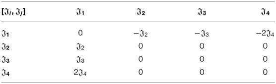
Table 1. Commutator table of the vector fields of system (3).

TABLE 2

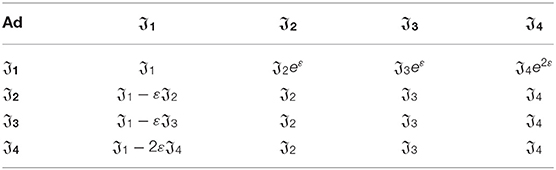
Table 2. Adjoint table of the vector fields of system (3).

Based on Tables 1, 2, system (3) has the following optimal system [3, 32]

$\begin{array}{ll}(\text{i}){𝔍}_1;(\text{ii}){𝔍}_2+\alpha {𝔍}_3+\beta {𝔍}_4;(\text{iii}){𝔍}_3+\chi {𝔍}_4;(\text{iv}){𝔍}_4,& (14)\end{array}$

where α, β, and χ are arbitrary constants.

Symmetry Reductions and Invariant Solutions

Based on the optimal system (14), our major goal is to deal with the similarity reductions and invariant solutions for system (3).

Subalgebra 𝔍₁

The characteristic equations of subalgebra 𝔍₁ can be written as

$\begin{array}{ll}\frac{dx}{x}=\frac{dy}{y}=\frac{dt}{\frac{2}{{\delta }_1(t)}\int {\delta }_1(t)dt}=\frac{du}{u}=\frac{dv}{v}.& (15)\end{array}$

Solving these equations yields the four similarity variables

$\begin{array}{l}r=x{\left({\displaystyle \int }{\delta }_1(t)dt\right)}^{-\frac{1}{2}},s=y{\left({\displaystyle \int }{\delta }_1(t)dt\right)}^{-\frac{1}{2}},\\ u=F(r,s)·{\left({\displaystyle \int }{\delta }_1(t)dt\right)}^{\frac{1}{2}},v=H(r,s)·{\left({\displaystyle \int }{\delta }_1(t)dt\right)}^{\frac{1}{2}},& (16)\end{array}$

and solving the constrained conditions (9), we get

$\begin{array}{l}{\delta }_2(t)=k_1{\delta }_1(t),{\delta }_3(t)=k_2{\delta }_1(t),\\ {\delta }_4(t)=k_3{\delta }_1(t){\left({\displaystyle \int }{\delta }_1(t)dt\right)}^{-2},& (17)\end{array}$

where k₁, k₂, and k₃ are arbitrary constants. These variables reduce system (3) to the following (1+1)-dimensional PDEs

$\begin{array}{ll}\{\begin{array}{l}F-r{F}_r-s{F}_s+2H_{rr}+2k_1{H}_{ss}+2k_2{H}_{rs}\\ +2k_3(F^{2}H+H^3)=0,\\ -H+r{H}_r+s{H}_s+2F_{rr}+2k_1{F}_{ss}+2k_2{F}_{rs}+2k_3(F^3\\ +F{H}^2)=0.\end{array}& (18)\end{array}$

Subalgebra 𝔍₁ does not give any group-invariant solutions.

Subalgebra 𝔍₂ + α𝔍₃ + β𝔍₄

The similarity variables of this generator are

$\begin{array}{r}r=\alpha x-y,s=\beta x-{\displaystyle \int }{\delta }_1(t)dt,\\ u=F(r,s),v=H(r,s),& (19)\end{array}$

and solving the constrained conditions (9), we get

$\begin{array}{ll}{\delta }_2(t)=k_1{\delta }_1(t),{\delta }_3(t)=k_2{\delta }_1(t),{\delta }_4(t)=k_3{\delta }_1(t),& (20)\end{array}$

where k_i(i = 1, 2, 3, 4) are arbitrary constants. Substituting Equations (19) and (20) into (3), we have

$\begin{array}{ll}\{\begin{array}{l}{F}_s-({\alpha }^2+k_1-\alpha k_2)H_{rr}-{\beta }^2{H}_{ss}-(2\alpha \beta -\beta k_2)H_{rs}\\ -k_3(F^{2}H+H^3)=0,\\ H_s+({\alpha }^2+k_1-\alpha k_2)F_{rr}+{\beta }^2{F}_{ss}+(2\alpha \beta -\beta k_2)F_{rs}\\ +k_3(F^3+F{H}^2)=0.\end{array}& (21)\end{array}$

For solving Equation (21), we use the transformation ζ = r − κs, F = f(ζ), H = h(ζ), where κ is an arbitrary constant, and then (21) can be reduced to the following ODEs

$\begin{array}{ll}\{\begin{array}{l}-\kappa f^{\prime }+(2\alpha \beta \kappa -\beta k_2\kappa -{\beta }^2{\kappa }^2-{\alpha }^2-k_1+\alpha k_2)h^{″}\\ -k_3(f^{2}h+h^3)=0,\\ -\kappa h^{\prime }-(2\alpha \beta \lambda -\beta k_2\lambda -{\beta }^2{\lambda }^2-{\alpha }^2-k_1+\alpha k_2)f^{″}\\ +k_3(f^3+f{h}^2)=0.\end{array}& (22)\end{array}$

Solving Equation (22) yields

$\begin{array}{ll}\{\begin{array}{l}f=-B_1\\ +A_{1}tan\left(r-\frac{4\alpha \beta -2\beta k_2+1-\sqrt{4{\beta }^2(k_2^2-4k_1)+4\beta (2\alpha -k_2)+1}}{4{\beta }^2}s\right),\\ h=A_1\\ +B_{1}tan\left(r-\frac{4\alpha \beta -2\beta k_2+1-\sqrt{4{\beta }^2(k_2^2-4k_1)+4\beta (2\alpha -k_2)+1}}{4{\beta }^2}s\right),\end{array}& (23)\end{array}$

and

$\begin{array}{ll}\{\begin{array}{l}f=-B_1\\ +A_{1}cot\left(r-\frac{4\alpha \beta -2\beta k_2+1-\sqrt{4{\beta }^2(k_2^2-4k_1)+4\beta (2\alpha -k_2)+1}}{4{\beta }^2}s\right),\\ h=A_1\\ +B_{1}cot\left(r-\frac{4\alpha \beta -2\beta k_2+1-\sqrt{4{\beta }^2(k_2^2-4k_1)+4\beta (2\alpha -k_2)+1}}{4{\beta }^2}s\right),\end{array}& (24)\end{array}$

where $k_3=-\frac{4\alpha \beta -2\beta k_2+1-\sqrt{4{\beta }^2(k_2^2-4k_1)+4\beta (2\alpha -k_2)+1}}{4{\beta }^2(A_1^2+B_1^2)}$ and A₁, B₁ are free parameters.

Based on Equations (19), (23), and (24), we obtain the following trigonometric function solutions for system (3)

$\begin{array}{ll}\{\begin{array}{l}u=-B_1\\ +A_{1}tan(\alpha x-y-\frac{4\alpha \beta -2\beta k_2+1-\sqrt{4{\beta }^2(k_2^2-4k_1)+4\beta (2\alpha -k_2)+1}}{4{\beta }^2}\\ (\beta x-\int {\delta }_1(t)dt)),\\ v=A_1\\ +B_{1}tan(\alpha x-y-\frac{4\alpha \beta -2\beta k_2+1-\sqrt{4{\beta }^2(k_2^2-4k_1)+4\beta (2\alpha -k_2)+1}}{4{\beta }^2}\\ (\beta x-\int {\delta }_1(t)dt)),\end{array}& (25)\end{array}$

and

$\begin{array}{ll}\{\begin{array}{l}u=-B_1\\ +A_{1}cot(\alpha x-y-\frac{4\alpha \beta -2\beta k_2+1-\sqrt{4{\beta }^2(k_2^2-4k_1)+4\beta (2\alpha -k_2)+1}}{4{\beta }^2}\\ (\beta x-\int {\delta }_1(t)dt)),\\ v=A_1\\ +B_{1}cot(\alpha x-y-\frac{4\alpha \beta -2\beta k_2+1-\sqrt{4{\beta }^2(k_2^2-4k_1)+4\beta (2\alpha -k_2)+1}}{4{\beta }^2}\\ (\beta x-\int {\delta }_1(t)dt)),\end{array}& (26)\end{array}$

where $k_3=-\frac{4\alpha \beta -2\beta k_2+1-\sqrt{4{\beta }^2(k_2^2-4k_1)+4\beta (2\alpha -k_2)+1}}{4{\beta }^2(A_1^2+B_1^2)}$ and A₁, B₁ are free parameters.

Subalgebra 𝔍₃ + χ𝔍₄

The similarity variables of this generator are

$\begin{array}{r}r=x,s=\chi y-{\displaystyle \int }{\delta }_1(t)dt,\\ u=F(r,s),v=H(r,s),& (27)\end{array}$

and solving the constrained conditions (9), we get

$\begin{array}{ll}{\delta }_2(t)=k_1{\delta }_1(t),{\delta }_3(t)=k_2{\delta }_1(t),{\delta }_4(t)=k_3{\delta }_1(t),& (28)\end{array}$

where k_i(i = 1, 2, 3, 4) are arbitrary constants. System (3) can then be transformed to

$\begin{array}{ll}\{\begin{array}{l}{F}_s-H_{rr}-{\chi }^2{k}_1{H}_{ss}-\chi k_2{H}_{rs}-k_3(F^{2}H+H^3)=0,\\ H_s+F_{rr}+{\chi }^2{k}_1{F}_{ss}+\chi k_2{F}_{rs}+k_3(F^3+F{H}^2)=0.\end{array}& (29)\end{array}$

For solving Equation (29), we use the transformation ζ = r − κs, F = f(ζ), H = h(ζ), where κ is an arbitrary constant; Equation (29) can then be written as

$\begin{array}{ll}\{\begin{array}{l}-\kappa f^{\prime }+(\chi k_2\kappa -{\chi }^2{\kappa }^2{k}_1-1)h^{″}-k_3(f^{2}h+h^3)=0,\\ -\kappa h^{\prime }-(\chi k_2\kappa -{\chi }^2{\kappa }^2{k}_1-1)f^{″}+k_3(f^3+f{h}^2)=0.\end{array}& (30)\end{array}$

To obtain the solutions of Equation (30), we shall apply the $\left(\frac{G^{\prime }}{G}\right)$ method, as described in [33].

Let us consider the solutions of (30), as

$\begin{array}{ll}f={\displaystyle \sum _{i=0}^n}{A}_i{\left(\frac{G^{\prime }}{G}\right)}^i,h={\displaystyle \sum _{i=0}^m}{B}_i{\left(\frac{G^{\prime }}{G}\right)}^i.& (31)\end{array}$

By balancing the highest order derivative term and non-linear term in (30), we obtain m = n = 1, and G = G(ζ) satisfies second-order ODE

$\begin{array}{l}{G}^{″}+\lambda G^{\prime }+\mu G=0.\end{array}$

Solving Equation (30), we obtain

$\begin{array}{r}\mu =\frac{{\lambda }^2(A_1^2+B_1^2)+4B_0(B_0-\lambda B_1)}{4A_1^2},\\ A_0=\frac{\lambda (A_1^2+B_1^2)-2B_0{B}_1}{2A_1},\kappa =\frac{k_3(A_1^2+B_1^2)(2B_0-\lambda B_1)}{2A_1},\\ k_1=\frac{-2A_1((A_1^2+B_1^2)(\lambda \chi B_1{k}_2{k}_3-2\chi A_1{B}_0{k}_2{k}_3+2A_1{k}_3)+2A_1)}{{\chi }^2{k}_3^2{(\lambda A_1^2{B}_1+\lambda B_1^3-2A_1^2{B}_0-2B_0{B}_1^2)}^2},& (32)\end{array}$

where λ, χ, d₁, B₀, B₁, k₂, and k₃ are arbitrary constants.

Substituting (32) into (30), we obtain two types of solutions of (30), as follows:

When λ² − 4μ > 0,

$\begin{array}{ll}\{\begin{array}{l}f=\frac{\lambda B_1-2B_0}{2i}\times \left(\frac{C_{1}cosh\left(\frac{1}{2}\sqrt{{\lambda }^2-4\mu }\zeta \right)+C_{2}sinh\left(\frac{1}{2}\sqrt{{\lambda }^2-4\mu }\zeta \right)}{C_{1}sinh\left(\frac{1}{2}\sqrt{{\lambda }^2-4\mu }\zeta \right)+C_{2}cosh\left(\frac{1}{2}\sqrt{{\lambda }^2-4\mu }\zeta \right)}\right)\\ -\frac{\lambda (\lambda B_1-2B_0)}{2i\sqrt{{\lambda }^2-4\mu }}-\frac{\lambda B_0-2\mu B_1}{i\sqrt{{\lambda }^2-4\mu }},\\ h=\frac{B_1}{2}\sqrt{{\lambda }^2-4\mu }\times \left(\frac{C_{1}cosh\left(\frac{1}{2}\sqrt{{\lambda }^2-4\mu }\zeta \right)+C_{2}sinh\left(\frac{1}{2}\sqrt{{\lambda }^2-4\mu }\zeta \right)}{C_{1}sinh\left(\frac{1}{2}\sqrt{{\lambda }^2-4\mu }\zeta \right)+C_{2}cosh\left(\frac{1}{2}\sqrt{{\lambda }^2-4\mu }\zeta \right)}\right)\\ -\frac{\lambda B_1}{2}+B_0,\end{array}& (33)\end{array}$

where

$\begin{array}{r}{k}_1=\frac{\begin{array}{l}2k_3(\lambda B_0{B}_1-\mu B_1^2-B_0^2)+{\lambda }^2-4\mu +2i\chi k_2{k}_3(\lambda B_0{B}_1\\ -\mu B_1^2-B_0^2)\sqrt{{\lambda }^2-4\mu }\end{array}}{4{\chi }^2{k}_3^2{(\lambda B_0{B}_1-\mu B_1^2-B_0^2)}^2},\\ \zeta =r-\frac{2k_3(\lambda B_0{B}_1-\mu B_1^2-B_0^2)}{i\sqrt{{\lambda }^2-4\mu }}s,\lambda ,\mu ,\chi ,B_0,B_1,\\ C_1,C_2,k_2,\text{and }{k}_3\text{ are arbitrary constants}.\end{array}$

When λ² − 4μ < 0,

$\begin{array}{ll}\{\begin{array}{l}f=\frac{\lambda B_1-2B_0}{2}\times \left(\frac{C_{1}cosh\left(\frac{1}{2}\sqrt{4\mu -{\lambda }^2}\zeta \right)-C_{2}sinh\left(\frac{1}{2}\sqrt{4\mu -{\lambda }^2}\zeta \right)}{C_{1}sinh\left(\frac{1}{2}\sqrt{4\mu -{\lambda }^2}\zeta \right)+C_{2}cosh\left(\frac{1}{2}\sqrt{4\mu -{\lambda }^2}\zeta \right)}\right)\\ -\frac{\lambda (\lambda B_1-2B_0)}{2\sqrt{4\mu -{\lambda }^2}}-\frac{\lambda B_0-2\mu B_1}{\sqrt{4\mu -{\lambda }^2}},\\ h=\frac{B_1}{2}\sqrt{4\mu -{\lambda }^2}\times \left(\frac{C_{1}cosh\left(\frac{1}{2}\sqrt{4\mu -{\lambda }^2}\zeta \right)-C_{2}sinh\left(\frac{1}{2}\sqrt{4\mu -{\lambda }^2}\zeta \right)}{C_{1}sinh\left(\frac{1}{2}\sqrt{4\mu -{\lambda }^2}\zeta \right)+C_{2}cosh\left(\frac{1}{2}\sqrt{4\mu -{\lambda }^2}\zeta \right)}\right)\\ -\frac{\lambda B_1}{2}+B_0,\end{array}& (34)\end{array}$

where

$\begin{array}{l}{k}_1=\frac{\begin{array}{l}2k_3(\lambda B_0{B}_1-\mu B_1^2-B_0^2)+{\lambda }^2-4\mu +2\chi k_2{k}_3(\lambda B_0{B}_1\\ -\mu B_1^2-B_0^2)\sqrt{4\mu -{\lambda }^2}\end{array}}{4{\chi }^2{k}_3^2{(\lambda B_0{B}_1-\mu B_1^2-B_0^2)}^2},\\ \zeta =r-\frac{2k_3(\mu B_1^2+B_0^2-\lambda B_0{B}_1)}{\sqrt{{\lambda }^2-4\mu }}s,\lambda ,\mu ,\chi ,B_0,B_1,C_1,C_2,k_2,\\ \text{\hspace{1em}\hspace{1em}\hspace{1em}\hspace{1em}\hspace{1em}\hspace{1em}\hspace{1em}\hspace{1em}\hspace{1em}\hspace{1em}\hspace{1em}and }{k}_3\text{ are arbitrary constants}.\end{array}$

Taking into account Equations (27), (33), and (34), we obtain the hyperbolic function solutions for system (3):

$\begin{array}{ll}\{\begin{array}{l}u=\frac{\lambda B_1-2B_0}{2i}\times \left(\frac{C_{1}cosh\left(\frac{1}{2}\sqrt{{\lambda }^2-4\mu }\zeta \right)+C_{2}sinh\left(\frac{1}{2}\sqrt{{\lambda }^2-4\mu }\zeta \right)}{C_{1}sinh\left(\frac{1}{2}\sqrt{{\lambda }^2-4\mu }\zeta \right)+C_{2}cosh\left(\frac{1}{2}\sqrt{{\lambda }^2-4\mu }\zeta \right)}\right)\\ -\frac{\lambda (\lambda B_1-2B_0)}{2i\sqrt{{\lambda }^2-4\mu }}-\frac{\lambda B_0-2\mu B_1}{i\sqrt{{\lambda }^2-4\mu }},\\ v=\frac{B_1}{2}\sqrt{{\lambda }^2-4\mu }\times \left(\frac{C_{1}cosh\left(\frac{1}{2}\sqrt{{\lambda }^2-4\mu }\zeta \right)+C_{2}sinh\left(\frac{1}{2}\sqrt{{\lambda }^2-4\mu }\zeta \right)}{C_{1}sinh\left(\frac{1}{2}\sqrt{{\lambda }^2-4\mu }\zeta \right)+C_{2}cosh\left(\frac{1}{2}\sqrt{{\lambda }^2-4\mu }\zeta \right)}\right)\\ -\frac{\lambda B_1}{2}+B_0,\end{array}& (35)\end{array}$

where λ² − 4μ > 0,

$\begin{array}{r}{k}_1=\frac{\begin{array}{l}2k_3(\lambda B_0{B}_1-\mu B_1^2-B_0^2)+{\lambda }^2-4\mu \\ +2i\chi k_2{k}_3(\lambda B_0{B}_1-\mu B_1^2-B_0^2)\sqrt{{\lambda }^2-4\mu }\end{array}}{4{\chi }^2{k}_3^2{(\lambda B_0{B}_1-\mu B_1^2-B_0^2)}^2},\\ \zeta =x-\frac{2k_3(\lambda B_0{B}_1-\mu B_1^2-B_0^2)}{i\sqrt{{\lambda }^2-4\mu }}\left(\chi y-{\displaystyle \int }{\delta }_1(t)dt\right),\\ \lambda ,\mu ,\chi ,B_0,B_1,C_1,C_2,k_2,\\ \text{and }{k}_3\text{are arbitrary constants}.\\ \{\begin{array}{l}u=\frac{\lambda B_1-2B_0}{2}\times \left(\frac{C_{1}cos\left(\frac{1}{2}\sqrt{4\mu -{\lambda }^2}\zeta \right)-C_{2}sin\left(\frac{1}{2}\sqrt{4\mu -{\lambda }^2}\zeta \right)}{C_{1}sin\left(\frac{1}{2}\sqrt{4\mu -{\lambda }^2}\zeta \right)+C_{2}cos\left(\frac{1}{2}\sqrt{4\mu -{\lambda }^2}\zeta \right)}\right)\\ -\frac{\lambda (\lambda B_1-2B_0)}{2\sqrt{4\mu -{\lambda }^2}}-\frac{\lambda B_0-2\mu B_1}{\sqrt{4\mu -{\lambda }^2}},\\ v=\frac{B_1}{2}\sqrt{4\mu -{\lambda }^2}\times \left(\frac{C_{1}cos\left(\frac{1}{2}\sqrt{4\mu -{\lambda }^2}\zeta \right)-C_{2}sin\left(\frac{1}{2}\sqrt{4\mu -{\lambda }^2}\zeta \right)}{C_{1}sin\left(\frac{1}{2}\sqrt{4\mu -{\lambda }^2}\zeta \right)+C_{2}cos\left(\frac{1}{2}\sqrt{4\mu -{\lambda }^2}\zeta \right)}\right)\\ -\frac{\lambda B_1}{2}+B_0,\end{array}& (36)\end{array}$

where λ² − 4μ < 0,

$\begin{array}{r}{k}_1=\frac{\begin{array}{l}2k_3(\lambda B_0{B}_1-\mu B_1^2-B_0^2)+{\lambda }^2-4\mu +2\chi k_2{k}_3(\lambda B_0{B}_1\\ -\mu B_1^2-B_0^2)\sqrt{4\mu -{\lambda }^2}\end{array}}{4{\chi }^2{k}_3^2{(\lambda B_0{B}_1-\mu B_1^2-B_0^2)}^2},\\ \zeta =x-\frac{2k_3(\mu B_1^2+B_0^2-\lambda B_0{B}_1)}{\sqrt{{\lambda }^2-4\mu }}\left(\chi y-{\displaystyle \int }{\delta }_1(t)dt\right),\\ \lambda ,\mu ,\chi ,B_0,B_1,C_1,C_2,k_2,\text{and }{k}_3\text{ are arbitrary constants}.\end{array}$

Subalgebra ${𝔍}_4=\frac{1}{{\delta }_1(t)}\frac{\partial }{\partial t}$

The similarity variables of this generator are

$\begin{array}{r}r=x,s=y,\\ u=F(r,s),v=H(r,s),& (37)\end{array}$

and solving the constrained conditions (9), we get

$\begin{array}{ll}{\delta }_2(t)=k_1{\delta }_1(t),{\delta }_3(t)=k_2{\delta }_1(t),{\delta }_4(t)=k_3{\delta }_1(t),& (38)\end{array}$

where k_i(i = 1, 2, 3) are arbitrary constants. Thus, system (3) can be transformed to

$\begin{array}{ll}\{\begin{array}{l}{H}_{rr}+k_1{H}_{ss}+k_2{H}_{rs}+k_3(F^{2}H+H^3)=0,\\ F_{rr}+k_1{F}_{ss}+k_2{F}_{rs}+k_3(F^3+F{H}^2)=0.\end{array}& (39)\end{array}$

For solving Equation (39), we use the transformation ζ = r − κs, F = f(ζ), H = h(ζ), where λ is an arbitrary constant, and then (39) can be reduced to the following ODEs

$\begin{array}{ll}\{\begin{array}{l}(1+{\kappa }^2{k}_1-\kappa k_2)h^{″}+k_3(f^{2}h+h^3)=0,\\ (1+{\kappa }^2{k}_1-\kappa k_2)f^{″}+k_3(f^3+f{h}^2)=0.\end{array}& (40)\end{array}$

Solving Equation (40) yields

$\begin{array}{ll}\{\begin{array}{l}f=C_{1}sin\left(r-\frac{k_2+\sqrt{4k_1{k}_3(C_1^2+C_2^2)+k_2^2-4k_1}}{2k_1}s\right)\\ -C_{2}cos\left(r-\frac{k_2+\sqrt{4k_1{k}_3(C_1^2+C_2^2)+k_2^2-4k_1}}{2k_1}s\right),\\ h=C_{2}sin\left(r-\frac{k_2+\sqrt{4k_1{k}_3(C_1^2+C_2^2)+k_2^2-4k_1}}{2k_1}s\right)\\ +C_{1}cos\left(r-\frac{k_2+\sqrt{4k_1{k}_3(C_1^2+C_2^2)+k_2^2-4k_1}}{2k_1}s\right),\end{array}& (41)\end{array}$

where C₁, C₂, k₁, k₂, and k₃ are arbitrary constants.

On combining Equations (37) and (41), we obtain the periodic function solutions for system (3):

$\begin{array}{ll}\{\begin{array}{l}u=C_{1}sin\left(x-\frac{k_2+\sqrt{4k_1{k}_3(C_1^2+C_2^2)+k_2^2-4k_1}}{2k_1}y\right)\\ -C_{2}cos\left(x-\frac{k_2+\sqrt{4k_1{k}_3(C_1^2+C_2^2)+k_2^2-4k_1}}{2k_1}y\right),\\ v=C_{2}sin\left(x-\frac{k_2+\sqrt{4k_1{k}_3(C_1^2+C_2^2)+k_2^2-4k_1}}{2k_1}y\right)\\ +C_{1}cos\left(x-\frac{k_2+\sqrt{4k_1{k}_3(C_1^2+C_2^2)+k_2^2-4k_1}}{2k_1}y\right),\end{array}& (42)\end{array}$

where C₁, C₂, k₁, k₂, and k₃ are arbitrary constants.

Non-linear Self-Adjointness and Conservation Laws

Conservation laws have been extensively researched due to their important physical significance. Many effective approaches have been proposed to construct conservation laws for NPDEs, such as Noether's theorem [34], the multiplier approach [35], and so on [36, 37]. Ibragimov [38, 39] proposed a new conservation theorem that does not require the existence of a Lagrangian and is based on the concept of an adjoint equation for NLPDEs. In this section, we will construct non-linear self-adjointness and conservation laws for vcHFSC equation (1).

Non-linear Self-Adjointness

Based on the method of constructing Lagrangians [38], we have the following formal Lagrangian ${L}$ in the symmetric form

$\begin{array}{l}{L}=ū[u_t+{\delta }_1(t)v_{xx}+{\delta }_2(t)v_{yy}+\frac{1}{2}{\delta }_3(t)v_{xy}\\ +\frac{1}{2}{\delta }_3(t)v_{yx}+{\delta }_4(t)(u^{2}v+v^3)]\\ +\bar{v}[-v_t+{\delta }_1(t)u_{xx}+{\delta }_2(t)u_{yy}+\frac{1}{2}{\delta }_3(t)u_{xy}\\ +\frac{1}{2}{\delta }_3(t)u_{yx}+{\delta }_4(t)(u^3+u{v}^2)],& (43)\end{array}$

where ū and $\bar{v}$ are two new dependent variables.

The adjoint system of system (3) is

$\begin{array}{ll}\{\begin{array}{l}{F}_1^{*}=\frac{\delta {L}}{\delta u}=0,\\ F_2^{*}=\frac{\delta {L}}{\delta v}=0,\end{array}& (44)\end{array}$

where

$\begin{array}{ll}\frac{\delta {L}}{\delta u}\text{=}\frac{\partial {L}}{\partial u}-D_t\frac{\partial {L}}{\partial u_t}+D_x{D}_x\frac{\partial {L}}{\partial u_{xx}}+D_x{D}_y\frac{\partial {L}}{\partial u_{xy}}+D_y{D}_y\frac{\partial {L}}{\partial u_{yy}},& (45)\end{array}$

$\begin{array}{ll}\frac{\delta {L}}{\delta v}\text{=}\frac{\partial {L}}{\partial v}-D_t\frac{\partial {L}}{\partial v_t}+D_x{D}_x\frac{\partial {L}}{\partial v_{xx}}+D_x{D}_y\frac{\partial {L}}{\partial v_{xy}}+D_y{D}_y\frac{\partial {L}}{\partial v_{yy}},& (46)\end{array}$

with D_x, D_y, and D_t the total differentiations with respect to x, y, and t.

For illustration, D_x can be expressed as

$\begin{array}{r}{D}_x=\frac{\partial }{\partial x}+u_x\frac{\partial }{\partial u}+v_x\frac{\partial }{\partial v}+u_{xx}\frac{\partial }{\partial u_x}+v_{xx}\frac{\partial }{\partial v_x}+u_{xt}\frac{\partial }{\partial u_t}\\ +v_{xt}\frac{\partial }{\partial v_t}+\cdots .\end{array}$

Substituting (43), (45), and (46) into (44), the adjoint system for system (3) is

$\begin{array}{ll}\{\begin{array}{l}{F}_1^{*}=-{ū}_t+{\delta }_1(t){\bar{v}}_{xx}+{\delta }_2(t){\bar{v}}_{yy}+{\delta }_3(t){\bar{v}}_{xy}\\ +2{\delta }_4(t)ūuv+{\delta }_4(t)\bar{v}(3u^2+v^2),\\ F_2^{*}={\bar{v}}_t+{\delta }_1(t){ū}_{xx}+{\delta }_2(t){ū}_{yy}+{\delta }_3(t){ū}_{xy}\\ +2{\delta }_4(t)\bar{v}uv+{\delta }_4(t)ū(u^2+3v^2).\end{array}& (47)\end{array}$

The system (3) is non-linear self-adjoint when adjoint system (47) satisfy the following conditions

$\begin{array}{ll}\{\begin{array}{l}{F_1^{*}|}_{ū=\varphi (x,y,t,u,v),\bar{v}=\psi (x,y,t,u,v)}={\lambda }_{11}{F}_1+{\lambda }_{12}{F}_2,\\ {F_2^{*}|}_{ū=\varphi (x,y,t,u,v),\bar{v}=\psi (x,y,t,u,v)}={\lambda }_{21}{F}_1+{\lambda }_{22}{F}_2,\end{array}& (48)\end{array}$

where ϕ(x, y, t, u, v)≠0 or ψ(x, y, t, u, v)≠0, and λ_ij (i, j = 1, 2) are undetermined coefficients.

Substituting the expressions of F_i (i = 1, 2) and $F_i^{*}$ (i = 1, 2) into (48), we obtain the following equations

$\begin{array}{l}({\lambda }_{12}-{\psi }_u)({\delta }_1(t)u_{xx}-{\delta }_2(t)u_{yy}-{\delta }_3(t)u_{xy})\\ -({\lambda }_{11}-{\psi }_v)({\delta }_1(t)v_{xx}+{\delta }_2(t)v_{yy}+{\delta }_3(t)v_{xy})\\ -({\lambda }_{11}+{\varphi }_u)u_t+({\lambda }_{12}-{\varphi }_v)v_t+{\psi }_{uv}(2{\delta }_1(t)u_x{v}_x\\ +2{\delta }_2(t)u_y{v}_y+{\delta }_3(t)u_x{v}_y+{\delta }_3(t)u_y{v}_x)\\ +{\psi }_{uu}({\delta }_1(t)u_x^2+{\delta }_2(t)u_y^2+{\delta }_3(t)u_x{u}_y)+{\psi }_{vv}({\delta }_1(t)v_x^2\\ +{\delta }_2(t)v_y^2+{\delta }_3(t)v_x{v}_y)\\ +(2{\delta }_1(t){\psi }_{xu}+{\delta }_3(t){\psi }_{yu})u_x+(2{\delta }_2(t){\psi }_{yu}+{\delta }_3(t){\psi }_{xu})u_y\\ +(2{\delta }_1(t){\psi }_{xv}+{\delta }_3(t){\psi }_{yv})v_x\\ +(2{\delta }_2(t){\psi }_{yv}+{\delta }_3(t){\psi }_{xv})v_y+{\delta }_1(t){\psi }_{xx}+{\delta }_2(t){\psi }_{yy}\\ +{\delta }_3(t){\psi }_{xy}-{\lambda }_{11}{\delta }_4(t)(u^{2}v+v^3)\\ -{\lambda }_{12}{\delta }_4(t)(u{v}^2+u^3)+2{\delta }_4(t)\varphi uv+3{\delta }_4(t)\psi u^2\\ +{\delta }_4(t)\psi v^2-{\varphi }_t=0,& (49)\end{array}$

$\begin{array}{l}-({\lambda }_{22}-{\varphi }_u)({\delta }_1(t)u_{xx}+{\delta }_2(t)u_{yy}+{\delta }_3(t)u_{xy})\\ -({\lambda }_{21}-{\varphi }_v)({\delta }_1(t)v_{xx}+{\delta }_2(t)v_{yy}+{\delta }_3(t)v_{xy})\\ -({\lambda }_{21}-{\psi }_u)u_t+({\lambda }_{22}+{\psi }_v)v_t+{\varphi }_{uv}(2{\delta }_1(t)u_x{v}_x\\ +2{\delta }_2(t)u_y{v}_y+{\delta }_3(t)u_x{v}_y+{\delta }_3(t)u_y{v}_x)\\ +{\varphi }_{uu}({\delta }_1(t)u_x^2+{\delta }_2(t)u_y^2+{\delta }_3(t)u_x{u}_y)+{\varphi }_{vv}({\delta }_1(t)v_x^2\\ +{\delta }_2(t)v_y^2+{\delta }_3(t)v_x{v}_y)\\ +(2{\delta }_1(t){\varphi }_{xu}+{\delta }_3(t){\varphi }_{yu})u_x\\ +(2{\delta }_2(t){\varphi }_{yu}+{\delta }_3(t){\varphi }_{xu})u_y+(2{\delta }_1(t){\varphi }_{xv}+{\delta }_3(t){\varphi }_{yv})v_x\\ +(2{\delta }_2(t){\varphi }_{yv}+{\delta }_3(t){\varphi }_{xv})v_y+{\delta }_1(t){\varphi }_{xx}+{\delta }_2(t){\varphi }_{yy}\\ +{\delta }_3(t){\varphi }_{xy}-{\lambda }_{21}{\delta }_4(t)(u^{2}v+v^3)\\ -{\lambda }_{22}{\delta }_4(t)(u{v}^2+u^3)+2{\delta }_4(t)\psi uv+3{\delta }_4(t)\varphi v^2\\ +{\delta }_4(t)\varphi u^2+{\psi }_t=0.& (50)\end{array}$

Solving the above systems, we have

$\begin{array}{ll}\varphi =-Cu,\psi =Cv,{\lambda }_{12}={\lambda }_{21}=0,{\lambda }_{11}=C,{\lambda }_{22}=-C.& (51)\end{array}$

Theorem 4.1. System (3) is non-linearly self-adjoint.

The formal Lagrangian corresponding to (43) reads as,

$\begin{array}{l}L=-Cu[u_t+{\delta }_1(t)v_{xx}+{\delta }_2(t)v_{yy}+\frac{1}{2}{\delta }_3(t)v_{xy}\\ +\frac{1}{2}{\delta }_3(t)v_{yx}+{\delta }_4(t)(u^{2}v+v^3)]\\ +Cv[-v_t+{\delta }_1(t)u_{xx}+{\delta }_2(t)u_{yy}+\frac{1}{2}{\delta }_3(t)u_{xy}\\ +\frac{1}{2}{\delta }_3(t)u_{yx}+{\delta }_4(t)(u^3+u{v}^2)].& (52)\end{array}$

Conservation Laws

In this section, we will construct the conservation laws for system (3) by Ibragimov's theorem. Next, we briefly review the notations used in the following sections. Let x = (x¹, x², …, xⁿ) be n independent variables, u = (u¹, u², …, u^m) be m dependent variables,

$\begin{array}{ll}X={\xi }_i(x,u,u_{(1)},\dots )\frac{\partial }{\partial x^i}+{\eta }_s(x,u,u_{(1)},\dots )\frac{\partial }{\partial u^s},& (53)\end{array}$

be a symmetry of m equations

$\begin{array}{ll}{F}_s(x,u,u_{(1)},\dots ,u_{(N)})=0,s=1,2,\dots ,m.& (54)\end{array}$

and the corresponding adjoint equation

$\begin{array}{r}{F}_s^{*}(x,u,v,u_{(1)},v_{(1)},\dots ,u_{(N)},v_{(N)})\\ =\frac{\delta (v^i{F}_i)}{\delta u^s}=0.s=1,2,\dots ,m.& (55)\end{array}$

Theorem 4.2. Any Lie point, Lie-Bäcklund and non-local symmetry X, as given in (53), of Equation (54) provides a conservation law for the system (54) and its adjoint system (55). The conserved vector is defined by

$\begin{array}{l}{T}^i={\xi }_i{L}+W^s\left[\frac{\partial {L}}{\partial u_i^s}-D_{x^j}\left(\frac{\partial {L}}{\partial u_{ij}^s}\right)+D_{x^j}{D}_{x^k}\left(\frac{\partial {L}}{\partial u_{ijk}^s}\right)-\cdots \right]\\ +D_{x^j}(W^s)\left[\frac{\partial {L}}{\partial u_{ij}^s}-D_{x^k}\left(\frac{\partial {L}}{\partial u_{ijk}^s}\right)+D_{x^k}{D}_{x^r}\left(\frac{\partial {L}}{\partial u_{ijkr}^s}\right)-\cdots \right]\\ +D_{x^j}{D}_{x^k}(W^s)\left[\frac{\partial {L}}{\partial u_{ijk}^s}-D_{x^r}\left(\frac{\partial {L}}{\partial u_{ijkr}^s}\right)+\cdots \right]+\cdots ,& (56)\end{array}$

where $W^s={\eta }_s-{\xi }_i{u}_i^s$ is the Lie characteristic function and ${L}={\displaystyle \sum _{i=1}^m}{v}^i{F}_i$ is the formal Lagrangian.

Based on the formula in Theorem 4.2, we next construct conserved vectors for system (3) by employing the formal Lagrangian (43) and the symmetry operator (10). For system (3), Equation (56) becomes the following form

$\begin{array}{l}{T}^x=\xi {L}-W^1\left[D_x\left(\frac{\partial {L}}{\partial u_{xx}}\right)+D_y\left(\frac{\partial {L}}{\partial u_{xy}}\right)\right]\\ +D_x(W^1)\left(\frac{\partial {L}}{\partial u_{xx}}\right)+D_y(W^1)\left(\frac{\partial {L}}{\partial u_{xy}}\right)\\ -W^2\left[D_x\left(\frac{\partial {L}}{\partial v_{xx}}\right)+D_y\left(\frac{\partial {L}}{\partial v_{xy}}\right)\right]+D_x(W^2)\left(\frac{\partial {L}}{\partial v_{xx}}\right)\\ +D_y(W^2)\left(\frac{\partial {L}}{\partial v_{xy}}\right)\\ =\xi {L}-W^{1}C({\delta }_1(t)v_x+\frac{1}{2}{\delta }_3(t)v_y)\\ +D_x(W^1)(C{\delta }_1(t)v)+D_y(W^1)\left(\frac{1}{2}C{\delta }_3(t)v\right)\\ +W^{2}C({\delta }_1(t)u_x+\frac{1}{2}{\delta }_3(t)u_y)-D_x(W^2)(C{\delta }_1(t)u)\\ -D_y(W^2)\left(\frac{1}{2}C{\delta }_3(t)u\right),& (57)\end{array}$

$\begin{array}{l}{T}^y=\eta {L}-W^1\left[D_x\left(\frac{\partial {L}}{\partial u_{yx}}\right)+D_y\left(\frac{\partial {L}}{\partial u_{yy}}\right)\right]\\ +D_x(W^1)\left(\frac{\partial {L}}{\partial u_{yx}}\right)+D_y(W^1)\left(\frac{\partial {L}}{\partial u_{yy}}\right)\\ -W^2\left[D_x\left(\frac{\partial {L}}{\partial v_{yx}}\right)+D_y\left(\frac{\partial {L}}{\partial v_{yy}}\right)\right]\\ +D_x(W^2)\left(\frac{\partial {L}}{\partial v_{yx}}\right)+D_y(W^2)\left(\frac{\partial {L}}{\partial v_{yy}}\right)\\ =\eta {L}-W^{1}C\left[\frac{1}{2}{\delta }_3(t)v_x+{\delta }_2(t)v_y\right]+D_x(W^1)\left(\frac{1}{2}C{\delta }_3(t)v\right)\\ +D_y(W^1)(C{\delta }_2(t)v)\\ +W^{2}C\left[\frac{1}{2}{\delta }_3(t)u_x+{\delta }_2(t)u_y\right]-D_x(W^2)\left(\frac{1}{2}C{\delta }_3(t)u\right)\\ -D_y(W^2)(C{\delta }_2(t)u),& (58)\end{array}$

$\begin{array}{r}{T}^t=\tau {L}+W^1\left(\frac{\partial {L}}{\partial u_t}\right)+W^2\left(\frac{\partial {L}}{\partial v_t}\right)=\tau \\ {L}-W^1(Cu)-W^2(Cv),& (59)\end{array}$

with

$\begin{array}{l}{W}^1=\Phi -\xi u_x-\eta u_y-\tau u_t,\\ W^2=\Omega -\xi v_x-\eta v_y-\tau v_t.\end{array}$

Case 1 ${𝔍}_1=x\frac{\partial }{\partial x}+y\frac{\partial }{\partial y}+\frac{2\int {\delta }_1(t)dt}{{\delta }_1(t)}\frac{\partial }{\partial t}+u\frac{\partial }{\partial u}+v\frac{\partial }{\partial v}$

The Lie characteristic functions for this operator are

$\begin{array}{ll}{W}^1=u-x{u}_x-y{u}_y-\frac{2\int {\delta }_1(t)dt}{{\delta }_1(t)}{u}_t,& (60)\end{array}$

$\begin{array}{ll}{W}^2=v-x{v}_x-y{v}_y-\frac{2\int {\delta }_1(t)dt}{{\delta }_1(t)}{v}_t.& (61)\end{array}$

The corresponding conservation laws are

$\begin{array}{l}{T}^x=-\frac{1}{2}C[2k_1{\delta }_1(t)(u{v}_{yy}-u_{yy}v)+k_2{\delta }_1(t)\\ (u{v}_{xy}-u_x{v}_y+u_y{v}_x-u_{xy}v)+2(u{u}_t+v{v}_t)]x\\ -\frac{1}{2}C[k_2{\delta }_1(t)(u_{yy}v-u{v}_{yy})+2{\delta }_1(t)\\ (u_{xy}v-u_y{v}_x-u{v}_{xy}+u_x{v}_y)]y\\ -\frac{1}{2}C\int {\delta }_1(t)dt[2k_2(u_{ty}v-u{v}_{ty}-u_t{v}_y+u_y{v}_t)\\ +4(u_{tx}v-u{v}_{tx}-u_t{v}_x+u_x{v}_t)]\\ -\frac{1}{2}C\left[k_2{\delta }_1(t)(u{v}_y-u_{y}v)+2{\delta }_1(t)(u{v}_x-u_{x}v)\right],& (62)\end{array}$

$\begin{array}{l}{T}^y=\frac{1}{2}C[2k_1{\delta }_1(t)(u{v}_{xy}+u_x{v}_y-u_y{v}_x-u_{xy}v)+k_2{\delta }_1(t)\\ (u{v}_{xx}-u_{xx}v)]x\\ +\frac{1}{2}C[2{\delta }_1(t)(u_{xx}v-u{v}_{xx})+k_2{\delta }_1(t)\\ (u_y{v}_x+u_{xy}v-u{v}_{xy}-u_x{v}_y)-2(u{u}_t+v{v}_t)]y\\ +\frac{1}{2}C\int {\delta }_1(t)dt[2k_2(u{v}_{tx}-u_{tx}v+u_t{v}_x-u_x{v}_t)\\ +4k_1(u{v}_{ty}-u_{ty}v+u_t{v}_y-u_y{v}_t)]\\ +\frac{1}{2}C\left[k_2{\delta }_1(t)(u_{x}v-u{v}_x)+2k_1{\delta }_1(t)(u_{y}v-u{v}_y)\right],& (63)\end{array}$

$\begin{array}{l}{T}^t=C\left[(u{u}_x+v{v}_x)x+(u{u}_y+v{v}_y)y-(u^2+v^2)\right]\\ -C\int {\delta }_1(t)dt[2k_1(u{v}_{yy}-u_{yy}v)\\ +2k_2(u{v}_{xy}-u_{xy}v)+2(u{v}_{xx}-u_{xx}v)].& (64)\end{array}$

Case 2 ${𝔍}_2=\frac{\partial }{\partial x}$

The Lie characteristic functions for this operator are

$\begin{array}{ll}{W}^1=-u_x,W^2=-v_x.& (65)\end{array}$

The corresponding conservation laws are

$\begin{array}{r}{T}^x=-\frac{1}{2}C[2{\delta }_2(t)(u{v}_{yy}-u_{yy}v)+{\delta }_3(t)\\ (u{v}_{xy}-u_{xy}v-u_x{v}_y+u_y{v}_x)+2(u{u}_t+v{v}_t)],& (66)\end{array}$

$\begin{array}{r}{T}^y=\frac{1}{2}C[2{\delta }_2(t)(u{v}_{xy}-u_{xy}v+u_x{v}_y-u_y{v}_x)+{\delta }_3(t)\\ (u{v}_{xx}-u_{xx}v)],& (67)\end{array}$

$\begin{array}{ll}{T}^t=C(u{u}_x+v{v}_x).& (68)\end{array}$

Case 3 ${𝔍}_3=\frac{\partial }{\partial y}$

The Lie characteristic functions for this operator are

$\begin{array}{ll}{W}^1=-u_y,W^2=-v_y.& (69)\end{array}$

The corresponding conservation laws are

$\begin{array}{r}{T}^x=\frac{1}{2}C[2{\delta }_1(t)(u{v}_{xy}-u_{xy}v-u_x{v}_y+u_y{v}_x)+{\delta }_3(t)\\ (u{v}_{yy}-u_{yy}v)],& (70)\end{array}$

$\begin{array}{r}{T}^y=\frac{1}{2}C[2{\delta }_1(t)(u_{xx}v-u{v}_{xx})-{\delta }_3(t)\\ (u{v}_{xy}-u_{xy}v+u_x{v}_y-u_y{v}_x)-2(u{u}_t+v{v}_t)],& (71)\end{array}$

$\begin{array}{ll}{T}^t=C(u{u}_y+v{v}_y).& (72)\end{array}$

Case 4 ${𝔍}_4=\frac{1}{{\delta }_1(t)}\frac{\partial }{\partial t}$

The Lie characteristic functions for this operator are

$\begin{array}{ll}{W}^1=-\frac{1}{{\delta }_1(t)}{u}_t,W^2=-\frac{1}{{\delta }_1(t)}{v}_t.& (73)\end{array}$

The corresponding conservation laws are,

$\begin{array}{r}{T}^x=\frac{1}{2}C[k_2(u{v}_{ty}-u_{ty}v+u_t{v}_y-u_y{v}_t)\\ +2(u{v}_{tx}-u_{tx}v+u_t{v}_x-u_x{v}_t)],& (74)\end{array}$

$\begin{array}{r}{T}^y=\frac{1}{2}C[k_2(u{v}_{tx}-u_{tx}v+u_t{v}_x-u_x{v}_t)\\ +2k_1(u{v}_{ty}-u_{ty}v+u_t{v}_y-u_y{v}_t)],& (75)\end{array}$

$\begin{array}{r}{T}^t=C[k_1(u_{yy}v-u{v}_{yy})\\ +k_2(u_{xy}v-u{v}_{xy})+(u_{xx}v-u{v}_{xx})].& (76)\end{array}$

Results and Discussion

The Lie group method has been successfully used to establish the invariant solutions for the vcHFSC equation. Some results for the vcHFSC equation have been published in the literature. Huang et al. [26] used the Hirota bilinear method and found the bright and dark solitons to Equation (1). Peng [27] reported some new non-autonomous complex wave and analytic solutions to Equation (1) with the aid of the (G′/G)method. In this article, we constructed the trigonometric and hyperbolic function solutions to the studied equation. Compared with the solutions obtained in references [26, 27], our results are new. To better understand the characteristics of the obtained solutions, the 3D graphical illustrations are plotted in Figures 1–3.

FIGURE 1

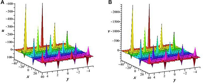
Figure 1. Plot of invariant solution (25) with δ₁(t) = sint, A₁ = 1, B₁ = 4, α = β = k₁ = 1, k₂ = 3 at t = 0. (A) Perspective view of the solution u. (B) Perspective view of the solution v.

FIGURE 2

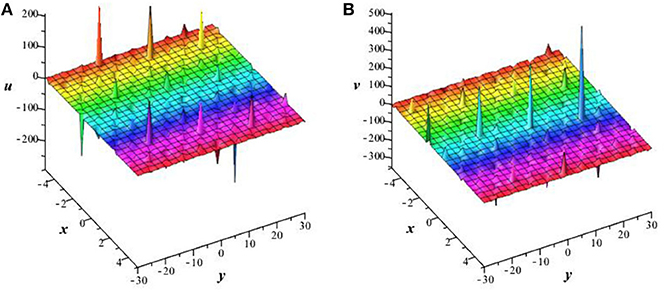
Figure 2. Plot of invariant solution (36) with δ₁(t) = 1, C₁ = 2, C₂ = 1, λ = μ = χ = 1, B₀ = B₁ = k₂ = k₃ = 1 at t = 5. (A) Perspective view of the solution u. (B) Perspective view of the solution v.

FIGURE 3

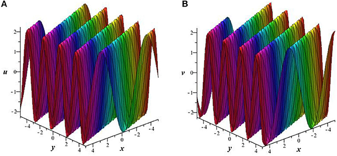
Figure 3. Plot of invariant solution (42) with C₁ = 1, C₂ = 2, k₁ = k₂ = k₃ = 1 at t = 0. (A) Perspective view of the solution u. (B) Perspective view of the solution v.

With the Lagrangian, we find that the vcHFSC equation is non-linearly self-adjoint. Furthermore, a new conservation theorem has been used to construct conservation laws for the vcHFSC equation. Based on the four infinitesimal generators, we obtained four conserved vectors. It worth noting that the conservation laws obtained in this article have been verified by Maple software.

Conclusion

In this research, the infinitesimal generators and Lie point symmetries of the vcHFSC equation have been investigated using the Lie group method. Based on the optimal system of one-dimensional subalgebras, four types of similarity reductions are presented. Taking similarity reductions into account, the invariant solutions are provided, including trigonometric and hyperbolic function solutions. Furthermore, conservation laws for the vcHFSC equation are derived by non-linear self-adjointness and a new conservation theorem.

Data Availability Statement

The original contributions presented in the study are included in the article; further inquiries can be directed to the corresponding author.

Author Contributions

The author confirms being the sole contributor of this work and has approved it for publication.

Funding

This work was supported by Shandong Provincial Government Grants, the National Natural Science Foundation of China-Shandong Joint Fund (No. U1806203), Program for Young Innovative Research Team in Shandong University of Political Science and Law, and the Project of Shandong Province Higher Educational Science and Technology Program (No. J18KA234).

Conflict of Interest

The author declares that the research was conducted in the absence of any commercial or financial relationships that could be construed as a potential conflict of interest.

Acknowledgments

We would like to express our sincerest thanks to the editor and the reviewers for their valuable suggestions and comments, which lead to further improvement of our original manuscript.

References

1. Mikhailov AV. The reduction problem and the inverse scattering method. Phys D. (1981) 3:73–117. doi: 10.1016/0167-2789(81)90120-2

CrossRef Full Text | Google Scholar

2. Olver PJ. Applications of Lie Groups to Differential Equations. Berlin: Springer (1993). doi: 10.1007/978-1-4612-4350-2

CrossRef Full Text | Google Scholar

3. Ovsiannikov LV. Group Analysis of Differential Equations. Cambridge: Academic (1982). doi: 10.1016/B978-0-12-531680-4.50012-5

CrossRef Full Text | Google Scholar

4. Bluman GW, Cheviakov AF, Anco SC. Applications of Symmetry Methods to Partial Differential Equations. Berlin: Springer (2010). doi: 10.1007/978-0-387-68028-6

CrossRef Full Text | Google Scholar

5. Hirota R, Satsuma J. Soliton solutions of a coupled Korteweg-de Vries equation. Phys Lett A. (1981) 85:407–8. doi: 10.1016/0375-9601(81)90423-0

CrossRef Full Text | Google Scholar

6. Ma WX. Lump solutions to the Kadomtsev-Petviashvili equation. Phys Lett A. (2015) 379:1975–8. doi: 10.1016/j.physleta.2015.06.061

CrossRef Full Text | Google Scholar

7. Fan EG. Extended Tanh-function method and its applications to nonlinear equations. Phys Lett A. (2000) 277:212–8. doi: 10.1016/S0375-9601(00)00725-8

CrossRef Full Text | Google Scholar

8. Abdou MA. The extended tanh method and its applications for solving nonlinear physical models. Appl Math Comput. (2010) 190:988–96. doi: 10.1016/j.amc.2007.01.070

CrossRef Full Text | Google Scholar

9. Wazwaz AM. The extended tanh method for the Zakharov-Kuznetsov (ZK) equation, the modified ZK equation, and its generalized forms. Comm Nonlinear Sci Numer Simul. (2008) 13:1039–47. doi: 10.1016/j.cnsns.2006.10.007

CrossRef Full Text | Google Scholar

10. Liu N, Liu YS. New multi-soliton solutions of a (3+1)-dimensional nonlinear evolution equation. Comput. Math. Appl. (2016) 71:1645–54. doi: 10.1016/j.camwa.2016.03.012

CrossRef Full Text | Google Scholar

11. Darvishi MT, Mohammad NA. Modification of extended homoclinic test approach to solve the (3+1)-dimensional potential-YTSF equation. Chin Phys Lett. (2011) 28:040201. doi: 10.1088/0256-307X/28/4/040202

CrossRef Full Text | Google Scholar

12. Wang CJ, Dai ZD, Lin L. Exact three-wave solution for higher dimensional KdV-type equation. Appl Math Comput. (2010) 216:501–5. doi: 10.1016/j.amc.2010.01.057

CrossRef Full Text | Google Scholar

13. Abdou MA. The extended F-expansion method and its application for a class of nonlinear evolution equations. Chaos Solitons Fractals. (2007) 31:95–104. doi: 10.1016/j.chaos.2005.09.030

CrossRef Full Text | Google Scholar

14. Emmanuel Y. The extended F-expansion method and its application for solving the nonlinear wave, CKGZ, GDS, DS and GZ equations. Phys Lett A. (2005) 340:149–60. doi: 10.1016/j.physleta.2005.03.066

CrossRef Full Text | Google Scholar

15. Liu N, Liu YS. Homoclinic breather wave, rouge wave and interaction solutions for a (3+1)-dimensional KdV-type equation. Phys Scr. (2019) 94:035201. doi: 10.1088/1402-4896/aaf654

CrossRef Full Text | Google Scholar

16. Liu N, Liu YS. Lump solitons and interaction phenomenon to a (3+1)-dimensional Kadomtsev-Petviashvili-Boussinesq-like equation. Mod Phys Lett. (2019) 33:1950395. doi: 10.1142/S0217984919503950

CrossRef Full Text | Google Scholar

17. Aliyu AI, Inc M, Yusuf A, Baleanu D, Bayram M. Dark-bright optical soliton and conserved vectors to the Biswas-Arshed equation with third-order dispersions in the absence of self-phase modulation. Front Phys. (2019) 7:28. doi: 10.3389/fphy.2019.00028

CrossRef Full Text | Google Scholar

18. Inc M, Aliyu AI, Yusuf A, Baleanu D. Optical solitons, conservation laws and modulation instability analysis for the modified nonlinear Schrödinger's equation for Davydov solitons. J Electromagn Waves Appl. (2018) 32:858–73. doi: 10.1080/09205071.2017.1408499

CrossRef Full Text | Google Scholar

19. Zhang LH, Xu FS. Conservation laws, symmetry reductions, and exact solutions of some Keller-Segel models. Adv Differ Equat. (2018) 2018:327. doi: 10.1186/s13662-018-1723-7

CrossRef Full Text | Google Scholar

20. Kaur L, Wazwaz AM. Painlevé analysis and invariant solutions of generalized fifth-order nonlinear integrable equation. Nonlinear Dyn. (2018) 94:2469–77. doi: 10.1007/s11071-018-4503-8

CrossRef Full Text | Google Scholar

21. Wang GW, Kara AH. A (2+1)-dimensional KdV equation and mKdV equation: symmetries, group invariant solutions and conservation laws. Phys Lett A. (2019) 383:728–31. doi: 10.1016/j.physleta.2018.11.040

CrossRef Full Text | Google Scholar

22. Wei GM, Lu YL, Xie YQ, Zheng WX. Lie symmetry analysis and conservation law of variable-coefficient Davey-Stewartson equation. Comput Math Appl. (2018) 75:3420–30. doi: 10.1016/j.camwa.2018.02.008

CrossRef Full Text | Google Scholar

23. Yusuf A, Inc M, Aliyu AI. Optical solitons possessing beta derivative of the Chen-Lee-Liu equation in optical fibers. Front. Phys. (2019) 7:34. doi: 10.3389/fphy.2019.00034

CrossRef Full Text | Google Scholar

24. Yusuf A, Inc M, Bayram M. Invariant and simulation analysis to the time fractional Abrahams-Tsuneto reaction diffusion system. Phys Scr. (2019) 94:125005. doi: 10.1088/1402-4896/ab373b

CrossRef Full Text | Google Scholar

25. Tchier F, Yusuf A, Aliyu AI. Soliton solutions and conservation laws for lossy nonlinear transmission line equation. Superlattices Microst. (2017) 107:320–36. doi: 10.1016/j.spmi.2017.04.003

CrossRef Full Text | Google Scholar

26. Huang QM, Gao YT, Jia SL. Bright and dark solitons for a variable-coefficient (2+1) dimensional Heisenberg ferromagnetic spin chain equation. Opt Quant Electron. (2018) 50:183. doi: 10.1007/s11082-018-1428-x

CrossRef Full Text | Google Scholar

27. Peng LJ. Nonautonomous complex wave solutions for the (2+1)-dimensional Heisenberg ferromagnetic spin chain equation with variable coefficients. Opt Quant Electron. (2019) 51:168. doi: 10.1007/s11082-019-1883-z

CrossRef Full Text | Google Scholar

28. Latha MM, Vasanthi CC. An integrable model of (2+1)-dimensional Heisenberg ferromagnetic spin chain and soliton excitations. Phys Scr. (2014) 89:065204. doi: 10.1088/0031-8949/89/6/065204

CrossRef Full Text | Google Scholar

29. Anitha T, Latha MM, Vasanthi CC. Dromions in (2+1) dimensional ferromagnetic spin chain with bilinear and biquadratic interactions. Phys A Stat Mech Appl. (2014) 415:105–15. doi: 10.1016/j.physa.2014.07.078

CrossRef Full Text | Google Scholar

30. Triki H, Wazwaz AM. New solitons and periodic wave solutions for the (2+1)-dimensional Heisenberg ferromagnetic spin chain equation. J Electromagn Wave. (2016) 30:788–94. doi: 10.1080/09205071.2016.1153986

CrossRef Full Text | Google Scholar

31. Tang GS, Wang SH, Wang GW. Solitons and complexitons solutions of an integrable model of (2+1)-dimensional Heisenberg ferromagnetic spin chain. Nonlinear Dyn. (2017) 88:2319–27. doi: 10.1007/s11071-017-3379-3

CrossRef Full Text | Google Scholar

32. Olver, P.J. Applications of Lie Groups to Differential Equations. New York, NY: Springer (1986). doi: 10.1007/978-1-4684-0274-2

CrossRef Full Text | Google Scholar

33. Wang ML, Li X, Zhang J. The $\left(\frac{G^{\prime }}{G}\right)$-expansion method and travelling wave solutions of nonlinear evolution equationsin mathematical physics. Phys Lett A. (2008) 372:417–23. doi: 10.1016/j.physleta.2007.07.051

PubMed Abstract | CrossRef Full Text | Google Scholar

34. Marwat DNK, Kara AH, Hayat T. Conservation laws and associated Noether type vector fields via partial Lagrangians and Noether's theorem for the liang equation. Int J Theor Phys. (2008) 47:3075–81. doi: 10.1007/s10773-008-9739-5

CrossRef Full Text | Google Scholar

35. Naz R. Conservation laws for some compacton equations using the multiplier approach. Appl Math Lett. (2012) 25:257–61. doi: 10.1016/j.aml.2011.08.019

CrossRef Full Text | Google Scholar

36. Bokhari AH, Al-Dweik AY, Kara AH, Mahomed FM, Zaman FD. Double reduction of a nonlinear (2+1) wave equation via conservation laws. Commun Nonlinear Sci Numer Simul. (2011) 16:1244–53. doi: 10.1016/j.cnsns.2010.07.007

CrossRef Full Text | Google Scholar

37. Sjöberg A. On double reductions from symmetries and conservation laws. Nonlinear Anal RWA. (2009) 10:3472–7. doi: 10.1016/j.nonrwa.2008.09.029

CrossRef Full Text | Google Scholar

38. Ibragimov NH. A new conservation theorem. J Math Anal Appl. (2007) 333:311–28. doi: 10.1016/j.jmaa.2006.10.078

CrossRef Full Text | Google Scholar

39. Ibragimov NH, Khamitovaa RS, Valenti A. Self-adjointness of a generalized Camassa-Holm equation. Appl Math Comput. (2011) 218:2579–83. doi: 10.1016/j.amc.2011.07.074

CrossRef Full Text | Google Scholar