 Carlo Pagani1*
 Martin Reuter2
- 1Université Grenoble Alpes, CNRS, LPMMC, Grenoble, France
- 2Institute of Physics (THEP), University of Mainz, Mainz, Germany
Background Independence is a sine qua non for every satisfactory theory of Quantum Gravity. If one tries to establish a corresponding notion of Wilsonian renormalization, or coarse graining, it presents a major conceptual and technical difficulty usually. In this paper, we adopt the approach of the gravitational Effective Average Action and demonstrate that, generically, coarse graining in Quantum Gravity and in standard field theories on a non-dynamical spacetime are profoundly different. By means of a concrete example, which, in connection with the cosmological constant problem, is also interesting in its own right, we show that the surprising and sometimes counterintuitive implications of Background Independent coarse graining are neither restricted to high energies nor to strongly non-perturbative regimes. In fact, while our approach has been employed in most studies of Asymptotic Safety, this particular ultraviolet behavior plays no essential role in the present context.
1. Introduction
The perhaps most remarkable feature of classical General Relativity is its ability to select and to describe the stage upon which all physics, both gravitational and non-gravitational, takes place. This stage, the set of all events, is what we call spacetime and try to model by means of (topological, differentiable, causal, pseudo-Riemannian,⋯) manifolds.
(1) The theory of General Relativity complies with the principle of Background Independence, which proclaims that no particular such “stage” should enjoy a privileged status a priori but rather should be a computable result of the dynamics. While this seems to be a natural and almost self-evident requirement for any classical or quantum theory of the physical world, all of our present non-gravitational physical theories violate Background Independence quite explicitly. In particular, the standard model of elementary particle physics is formulated on an externally prescribed and, thus, unexplained Minkowski spacetime.
In the realm of classical physics, it is well-known how to overcome this deficiency and to set up a matter-coupled gravity theory that determines the spacetime metric dynamically along with the matter fields. Historically, corresponding progress at the quantum level has been hampered by the non-renormalizability of perturbatively quantized General Relativity and the problems in finding a satisfactory microscopic theory of Quantum Gravity of any other sort.
As a result, two issues have gotten mixed up that, however, are quite independent logically, at least as long as no additional information is available. These are
(a) the difficulty of setting up a non-perturbative fundamental quantum theory of the gravitational (“spin-2”) interaction and
(b) the problem of repairing, in one way or another, the background dependence of the standard model and similar local quantum field theories on Minkowski space.
The respective classical variants of both problems are solved by General Relativity. A theory of “Quantum Gravity” in the modern sense of the word [1] likewise must address, and ultimately solve, the dynamics-related problem (a) as well as the Background Independence issue (b).
In the past, many discussions failed to appreciate (b) as an additional and independent point on the agenda, which has often led to severe misconceptions. One of them is the widespread prejudice that quantum gravity effects are numerically small and can be neglected for all practical purposes. It was nurtured by the observation that graviton corrections to standard model physics on a rigid Minkowski space tend to be numerically small, classically as well as quantum mechanically (to the extent they are under control). If one believes, however, that the ultimate Quantum Gravity theory is a Background Independent one, this kind of reasoning is flagrantly wrong.
Its deficiency is not so much that it leaves unexplained the Minkowskian spacetime, which we observe on the scale of our laboratories; the real flaw is that it closes its eyes toward the possibility that a state, which looks Minkowskian on laboratory scales, may well possess a completely different (metric, causal,⋯) structure on the shorter length scales from which we have no experimental information about gravity and the structure of spacetime. Instead, in a Background Independent theory, this structure is a computable prediction rather than a phenomenological input based upon incomplete experimental data.
(2) In this paper, we advocate the point of view that Quantum Gravity, regarded as a non-perturbative and Background Independent theory, can have substantial implications well beyond the areas envisaged in the past, questions of ultraviolet renormalizability, or tiny loop corrections due to gravitons.
To support this view, we analyzed the gravitational impact of vacuum fluctuations as an exemplary problem. It has the advantage that it allows for an almost perfect separation of the points (a) and (b) on our to do list. In fact, the dynamics-related part (a) is essentially trivial, while a number of unexpected results contradicting traditional beliefs follow from (b), that is, the imposition of Background Independence on an otherwise unspectacular dynamic.
(3) We employ a continuum approach to Quantum Gravity which quantizes pure or matter-coupled metric gravity in terms of the gravitational Average Action, a concept that is both covariant under diffeomorphisms and Background Independent [2]. This scale-dependent action functional satisfies a functional renormalization group equation. From very early on, it provided strong evidence for the theory's Asymptotic Safety, i.e., the non-perturbative renormalizability at a non-Gaussian ultraviolet fixed point [2–8], see [9, 10] for a general exposition and [10–25] for later extensions.
As a matter of principle, the Quantum Einstein Gravity constructed in this manner shares Background Independence and the choice of the metric as the field variables with General Relativity, though the microscopic action may well turn out different from the Einstein-Hilbert action. (See [9] for a detailed description of the various steps involved in the overall “Asymptotic Safety Program”).
While the gravitational Average Action does depend on a background metric besides the dynamical one, the setting complies with the requirements of Background Independence since the background metric is determined self-consistently by the so called “tadpole equation,” a generalization of Einstein's equation.
Self-consistent background metrics depend on the RG scale at which the Effective Average Action is evaluated. It follows that “going on-shell” at a given point of the renormalization group (RG) flow requires understanding two types of scale dependencies. First is the (familiar) direct dependence of the EAA on the RG scale, and second is an equally important indirect one associated to the re-adjustment of the self-consistent background metric as a solution to the scale dependent-tadpole condition.
The scale dependence of the Effective Average Action is due to a coarse graining or averaging process on the spacetime manifold. The occurrence of the indirect scale dependence is a concrete manifestation of the abstract principle of Background Independence.
(4) In this paper, we give a detailed account of the corresponding notion of Background Independent coarse graining, and we illustrate the discussion by studying explicitly the case where the self-consistent background metric is determined essentially by the cosmological constant and its RG flow.
To this end, we begin, in section 2, by reviewing the relevant aspects of the gravitational Effective Average Action (EAA). Then, in section 3, we turn to an object of central mathematical importance, namely the spectral flow induced by the Laplacian of the self-consistent background metric. As we shall see, such spectral flow acquires an explicit scale dependence.
Most importantly, this spectral flow tells us which field modes constitute the degree of freedom of the respective effective field theory at a given RG scale. We discover a surprising, seemingly paradoxical, behavior for a broad class of RG trajectories. A Background Independent theory of (matter coupled) quantum gravity looses rather than gains degrees of freedom at increasing energies in contrast with the expectation based on the off-shell formalism.
In section 4, we study to what extent the Background Independent theory can be reformulated as a theory of matter and gravity fluctuations on a rigid flat space. We will show that, in vacuo, such reformulation is possible only for a very short RG time since a “scale horizon” prevents one to go further.
Finally, in section 5 we use the insights gained to critically revisit, and refute, the argument leading to the naturalness problem of the energy density obtained by summing up the zero-point energies in quantum field theory.
Our presentation partly follows [26] to which the reader is referred for further information.
2. The Background Independent Effective Average Action
In this section we review some relevant properties of the gravitational EAA [2]. We focus mostly on properties that go beyond the standard EAA for matter fields on flat space, see [27–31].
(1) The EAA for Einstein gravity is defined by a functional integral over the metric μν. The integral is then expressed in terms of a fluctuation field μν and a background field μν. In the case of a linear split, the following relation holds: μν = μν − μν. The functional integral is characterized by a diffeomorphism invariant bare action S[, ⋯] and a suitable gauge-fixing term together with the associated Faddeev-Popov ghosts Cμ and [2]:
where is a multiplet of fields, with the dots denoting possible matter fields, and J ≡ (Ji) is a set of sources conjugate to them. On top of the bare action, the gauge-fixing, and the ghost terms, the total action includes a term ΔSk, the so-called cutoff action, which gives a mass of order k to the modes of which have a (covariantmomentum)2 smaller than k2.
(2) The background metric plays a crucial role in the present approach. By means of μν one constructs the associated Laplacian , with being the associated Levi-Civita connection. The spectrum of the Laplacian is determined by the following eigenvalue problem:
By expanding the fields on the associated eigen-modes {χn}, i.e., , we can view the functional integral as an integral over the coefficients an, . The cutoff action can then be expressed as a sum over the eigen-modes:
where R(0)(z) satisfies R(0)(0) = 1, and R(0)(∞) = 0, and is a monotonically decreasing function which smoothly “crosses over” near z = 1. As a consequence, a field eigen-mode χn(x) associated with an eigenvalue εn smaller than k2 is equipped with an effective mass term . The other modes remain essentially unaffected. This mechanism provides the IR cutoff that will cause the scale dependence of the EAA. In practice, it is convenient to rewrite (1.3) as , without resorting to an explicit mode decomposition, with the pseudo-differential operator
where Zk is a matrix acting in field space taking into account the different normalization of the fields.
(3) It is important to emphasize that the eigenvalue problem (1.2), the spectrum {εn[]}, and the set of eigenmodes, {χn[](x)}, depend on the background metric. This fact will play a crucial role later on.
(4) The gravitational EAA Γk[φ; ] is defined as the Legendre-Fenchel transform of Wk[J; ] with respect to the sources Ji, holding μν fixed and subtracting ΔSk[φ; ] from it. The EAA is a functional of the variables “dual” to J, viz. . The expectation value of the metric fluctuation is given by hμν ≡ 〈μν〉 = 〈μν〉−μν = gμν−μν, with gμν ≡ 〈μν〉.
(5) The path integral representation of Wk allows one to derive a number of properties satisfied by Γk, such as BRST- and split-symmetry Ward identities. In particular, one can derive the following exact functional RG equation (FRGE),
At least superficially, it has the same appearance as for matter theories [29–33]. Moreover, the following source-field relation (“effective Einstein equation”) holds
Instead of the pair (hμν, μν) one may employ gμν and μν as two independent variables and define
When setting the ghost fields to zero, , we write Γk[gμν, μν] ≡ Γk[hμν; μν], which is the proper vertex generating functional for the 1PI correlators of μν1. In this work, we limited ourselves to consider the EAA defined in this section. It could be interesting to extend our study to related functionals, see in particular [46], and pinpoint possible advantages and disadvantages of each choice.
For further details on the EAA, we refer to [2] and the comprehensive account in [9].
3. Scale-Dependent Spectra as a Diagnostic Tool
(1) In our argument, a central role will be played by the eigenbasis of □, henceforth denoted by Υ ≡ {χn}. The eigenmodes satisfy the -dependent eigenvalue equation
We refer to modes with as IR modes, while all others are UV modes. The lowest lying UV mode is the so called cutoff mode, χCOM. Its eigenvalue is either precisely equal to k2, or slightly larger if the spectrum is discrete. In the former case:
According to this division of the functions χn(x), the eigenbasis Υ ≡ Υ[] decomposes as
with ΥIR and ΥUV containing the IR and UV modes, respectively.
It needs to be emphasized that the decomposition (2.3) depends not only on the scale, k, but also on the background metric. Hence, dealing with a fixed functional
the attribute of being “UV” or “IR” depends on the μν-argument the functional is evaluated at. In particular the set of quantum numbers nCOM that characterizes the cutoff mode χCOM ≡ χn|n =nCOM depends on the background metric:
The spectrum of −□ is schematically represented in Figure 1 together with the cutoff mode at k = k1.
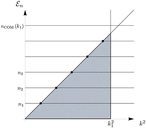
Figure 1. Representation of the spectral flow of −□ constructed via a scale independent background metric. This schematic representation shows a trivial spectral flow with the horizontal lines representing k-independent eigenvalues and the diagonal representing the identity k2 ↦ k2. The black dots denote the intersection points at which a mode is “integrated out.” At the scale k1, the IR degrees of freedom ΥIR[](k1) are associated to the eigenvalue lines passing through the shaded triangle.
(1) ΥIR[](k) and effective field theory. In the EAA-based quantization on a k-independent background metric the classification of the eigen-modes according to (2.3) can be interpreted physically:
(i) At a scale k = k1 the effect of the modes belonging to ΥUV[](k1) is encoded in the running (i.e., scale dependent) couplings that parametrize Γk1[φ; ]. Essentially, the modes in ΥUV[](k1) have been “integrated out.”
(ii) At the scale k1, the running couplings do not take into account the fluctuations of the modes in ΥIR[](k1), i.e., these modes have not been integrated out yet. It follows that Γk1 can be interpreted as an effective field theory that governs these modes at scales close to k1.
The term “effective field theory” has the following meaning for us. When employing the action functional Γk1 to compute some observable, only the modes belonging to ΥIR[](k1) remain to be quantized. Therefore, the scale k1 plays the role of an UV cutoff from an effective field theory point of view. All modes the effective field theory governs have eigenvalues .
Let us note that one may “integrate out” the IR-modes in ΥIR[](k1) by employing the FRGE and running the RG flow down to a lower scale (eventually k1 → 0). However, one may also “integrate out” these modes by any other suitable technique in principle.
(2) Self-consistent background geometries. Assume we solved the flow equation and obtained a certain RG trajectory k ↦ Γk, a curve on theory space. By differentiating the corresponding running action Γk[φ, ] with respect to φ, we may compute arbitrary proper vertices from which one may eventually calculate any arbitrary correlation function,
These correlators describe the dynamics of φ ≡ (hμν, ⋯)-fluctuations on a classical spacetime whose metric, μν, is enforced by unspecified external means. By appropriately changing the second argument of Γk[φ, ] and of its φ-derivatives, the RG trajectory informs us about the fluctuation dynamics on any given background geometry and at all scales.
A quantity of special interest is the one-point function 〈μν〉 since it determines the expectation value of the metric operator μν = μν + μν, i.e.,
In general, the expectation value (2.7) will be quite different from the background metric when the fields φ ≡ (hμν, ⋯) are quantized on a randomly chosen geometry.
Now, we go one step further and ask which metric expectation value the quantum system will realize when it is free from all external interferences. More concretely, if we quantize the set of fluctuation fields on a geometry with a given μν, we can ask which background(s) they would “like” most, in the sense that they dynamically produce a μν-expectation value that agrees precisely with the background metric prescribed. Such geometries are the called self-consistent geometries, and their metric is denoted . Hence,
Self-consistent background metrics can be found from the condition of a vanishing fluctuation one-point function, for historic reasons termed the tadpole condition. It comprises the equation
coupled to similar conditions where the differentiation is with respect to the other fluctuation fields.
In the following, it is of central importance that, generally, self-consistent backgrounds depend on the RG scale. By (2.9), it is clear that solutions inherit a certain k-dependence from Γk.
(3) Generalized RG trajectory. Henceforth, we assume that we solved the RG flow equation and have a certain trajectory k ↦ Γk in our hands. Furthermore, we assume that, using this running action as an input, we solved the tadpole equation and found a family of metrics labeled by k, or, stated differently, a curve in the space of metrics. It is natural therefore to refer to the map
as a generalized RG trajectory and to visualize it as a parametrized curve in the product of theory space with the space of metrics.
(4) Spectral flow. At every point of the generalized RG trajectory, we use the metric in order to construct the associated Laplacian . This results in a family of Laplacians whose members are distinguished by their respective value of k. Each family member gives rise to its own eigenvalue equation. It reads, for every value of k,
Solving the family of eigenvalue problems (2.11), we obtain a “curve of spectra,” i.e., a spectral flow,
and the corresponding eigenbasis, {χn(·;k)}.
If , the effective field equations implied by Γk admit the simple solution h = 0. The correlation functions (2.6) are thus taken “on-shell” when we evaluate them, separately for every k, at the self-consistent metric and simultaneously set h = 02. In this sense, the graviton n-point functions, for instance,
enjoy the property of being on-shell for each scale separately.
(5) Direct vs. indirect k-dependence. While on-shell at all points along the generalized RG trajectory, the n-point functions (2.13) possess a rather complicated scale dependence in general, which has two independent sources: the (naively expected) direct scale dependence, stemming from the k-dependence of the Γk, and the indirect scale dependence, caused by the continually changing, dynamically selected background metric.
The indirect scale dependence makes the physical interpretation of the coarse graining procedure rather non-trivial in general and striking surprises can occur, as we shall see.
(6) At the heart of Background Independent coarse graining. Recall that, when still “off-shell,” the Effective Average Action maps k-independent arguments onto a k-dependent number,
such that k2 is a cutoff in the spectrum of an operator, namely, −□, which is determined by the functional's second argument, .
By taking Γk and its h-derivatives on-shell, this operator gets concretely specified as , which possesses an explicit parametric dependence on k. k2 thus appears to be a cutoff in the spectrum of an operator that is k-dependent in itself.
With this somewhat confusing and paradoxical-looking situation, we have reached the very core of the Background Independent coarse graining: since physics (i.e., on-shell data) may not depend on any distinguished metric that was chosen ad hoc, spectral information of physical relevance is bound to come from operators which are determined dynamically [9].
The following steps are aiming at a first physical understanding of what it means to “coarse grain” under such conditions in a fully Background Independent fashion.
(7) Local IR-UV separation along the trajectory. We may assume that the eigenvalue problems (2.11) have been solved all the way along the generalized RG trajectory so that the spectral flow
can be analyzed explicitly. At first, we determine the cutoff modes of all the spectra occurring on the trajectory. At a given scale, say k = k1, we require that
and solve this condition for nCOM ≡ nCOM(k1). Equation (2.16) determines the label associated to the cutoff mode in the spectrum of the (on-shell!) background Laplacian at a given point of the theory space, which is visited by the RG flow when k = k1. When the spectrum is discrete, the cutoff mode corresponds to the smallest eigenvalue nCOM(k1) equal to or above .
Furthermore, we distribute the modes of the eigenbasis {χn(·;k1)} over two sets, putting those with eigenvalues n(k1) ≥ nCOM(k1)(k1) and n(k1) < nCOM(k1)(k1) into the sets ΥUV(k1) and ΥIR(k1), respectively.
By performing the outlined algorithm for all k1, one can construct the map k ↦ nCOM(k) or, more explicitly, k ↦ χnCOM(·;k). In the same manner, we can construct the “curves” k ↦ ΥUV/IR(k), and the decomposition of the eigenbasis,
which replaces (2.3) when going on-shell.
(8) Spectral flow and mode reshuffling. In Figure 2, we sketch a typical spectral flow of the kind that will arise later in our example. The trajectory's curve parameter k is on the horizontal axis, while two specific values, k = k1 and k = k2, are represented by two vertical lines. Figure 2 is analogous to Figure 1, the difference being that the eigenvalues εn are replaced by n(k). We refer to the k-dependence of the spectrum {n(k)} as the spectral flow induced by the (scale dependent) self-consistent background metric.
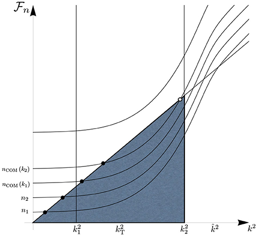
Figure 2. Schematic sketch of a non-trivial spectral flow.
(8.1) The cutoff mode at the scale k = k1 can be determined as follows. First one identifies all the intersection points between the graphs n(k) and the vertical line k = k1. The modes are then separated into two sets, i.e., ΥUV(k1) and ΥIR(k1), according to whether the intersection point lies above or exactly on the diagonal or below the diagonal, respectively.
The cutoff mode is defined as the mode associated to the smallest eigenvalue in ΥUV(k1). At the scale k = k1, the cutoff mode is labeled by nCOM(k1) as illustrated in Figure 2.
The mode carrying the label n = nCOM(k1), k1 fixed, is associated to a scale dependent eigenvalue nCOM(k1)(k). For values k ≠ k1, this mode plays no special role in general.
(8.2) As we explained, the effective action Γk|k =k1 governs the degrees of freedom associated to the modes in ΥIR(k1). These latter modes correspond to the eigenvalues passing within the shaded area to the left of the vertical k = k1-line in Figure 2. At scales lower than k1 these eigenvalues intersect the diagonal only once. The intersection is marked by a black dot similarly to the case of constant εn displayed in Figure 1.
This behavior can be interpreted as follows. By lowering k1, the vertical k = k1-line sweeps over one of the black dots on the diagonal. This implies that the associated mode is moved from ΥIR(k1) to ΥUV(k1). At first sight, one may suspect that this is what has to be expected in general since by lowering the cutoff one “integrates out” more and more modes.
(8.3) However, this picture changes dramatically at higher scales. Let us consider the scale k = k2, in Figure 2. As we shall see explicitly later on, the crucial point is that, if the cosmological constant increases with k rapidly enough, then the graph of an eigenvalue n(k) may intersects the diagonal more than once below k2. In Figure 2, we observe eigenvalues both entering and exiting from the shaded area to the left of the vertical k2-line, and the intersection points are marked by black dots or open circles accordingly. By lowering k2, it is possible for the k2-line to sweep over an open circle. This implies that a certain mode has changed its UV/IR status. However, this time, the mode moved from ΥUV(k2) to ΥIR(k2)!
At first glance, such behavior appears paradoxical and may seem “unphysical.” Indeed, we normally expect that, by integrating out further field modes, we are actually relocating them from the set ΥIR to the set ΥUV. In the present case, however, the opposite happens and a UV-mode in ΥUV becomes an IR-mode in ΥIR by lowering the RG scale.
(8.4) This conundrum is solved by recalling that the standard expectation, i.e., (klowered) ⇔ (mode transferΥIR → ΥUV), is valid for k-independent (off-shell) field arguments of the functional Γk[φ; ]. It must be emphasized that, during the computation of the EAA, this expectation holds true also in the present case. Such unexpected spectral behavior is due to the fact that, when the fields are taken on-shell and one employs the self-consistent background, they acquire a further scale dependence, which causes this non-trivial spectral flow.
It follows that there is nothing “unphysical” if, by lowering the value of k2, one observes a transition ΥUV → ΥIR. Actually, such transition encodes the physically important fact that the effective field theory described by Γk has gained a degree of freedom, whose fluctuations have not been taken into account in the values of the renormalized couplings in Γk.
As displayed in Figure 2, by lowering k further, the new IR-mode crosses the diagonal again and eventually becomes a UV-mode.
(9) Illustrative example: Einstein-Hilbert truncation. Let us pause for a moment and introduce an approximation that will be invoked for illustrative purposes in the following.
We truncate the gravity action to the Einstein-Hilbert form, and we either consider pure gravity, or matter coupled gravity in situations where the matter stress tensor in the effective field equation plays no significant role (at least at the level of the qualitative discussion we present here).
As a result, the tadpole condition (2.9) happens to assume the form of the classical Einstein equation in vacuo with a scale dependent cosmological constant:
Herein, k ↦ Λk is one of the functions that constitute the RG trajectory on theory space.
(i) As for the solution to Equation (2.18), we focus on the instructive, yet technically simple, class of solutions of the scaling type:
Here is an arbitrary solution to (2.18) for the cosmological constant Λ0. (Instead of the reference point k = 0, any other would do as well).
(ii) It is easy to determine the spectral flow caused by the k-dependence of the self-consistent background metric (2.19):
Moving along the generalized RG trajectory, the eigenvalues n(k) get rescaled, while the eigenfunctions remain unaltered.
(iii) For every fixed spectrum occurring along the trajectory we must determine the cutoff mode, i.e., the label nCOM ≡ nCOM(k). It is easy to show that this can be done by the following two-step algorithm:
• Determine the cutoff mode in the reference spectrum obtained with Λ0. In this case, denote the cutoff by q2 rather than, as usual, k2. Set up the equation
and solve it for nCOM. Denote the result by
thus defining the function .
• We would like to solve
Upon defining the function q (k) by
the solution to the problem (2.24) can be found in terms of the above as follows:
In the discussion of Figure 2, we have determined this k-dependence of nCOM by graphical means.
(10) Illustrative example: S4 spacetimes. Assuming a positive cosmological constant, the maximally symmetric solution to the (Euclidean) Einstein equation (2.18) is a sphere S4. Its radius follows from , i.e., , implying
The radius can be thought of as the Euclidean analog of the Hubble length.
(i) On S4, the eigenmodes of the tensor Laplacian are labeled by a positive integer, n, and a set of further quantum numbers the associated eigenvalue is independent of. The latter generalize the familiar magnetic quantum number m that appears as a label of the spherical harmonics Yl,m, i.e., the scalar eigenfunctions on S2, while the former is analogous to l which determines the eigenvalue, l (l + 1). For not too small values of n, the eigenvalues of the S4 harmonics, for tensors of any rank, are given by n2/r2, whence for the radius ,
The approximation behind Equation (2.28) is analogous to replacing l (l + 1) with l2 in the S2 case. Its advantage is that it is valid for tensors of any rank, contrary to the exact formula [47–50]. For the purposes of the present discussion we do not loose any relevant information by specializing for n ≫ 1. In fact, treating n as a large, quasi-continuous number also helps avoiding a number of inessential technicalities.
(ii) Using (2.27) and (2.28), the above algorithm yields the following answer for the quantum number of the cutoff mode:
Herein, q (k) is given by Equation (2.25), which we rewrite in the suggestive form
where is the dimensionless cosmological constant in cutoff units.
(11) The generic semiclassical RG trajectory. To go on and study the contents of (2.29), (2.30) we must pick an RG trajectory which then supplies a concrete function k ↦ Λk. In this paper, we focus on the semiclassical regime below the Planck scale (k ≲ mPl), where qualitatively the k-dependence of Λk is essentially the same for a large class of trajectories in pure gravity and also in matter-coupled gravity with many different matter systems. It reads, with constants Λ0 and ℓ,
The concomitant running of Newton's constant is trivial, Gk = G0 = const. This behavior applies in particular to the semiclassical regime of the Type IIIa trajectories in pure Quantum Einstein Gravity, see Figure 3.
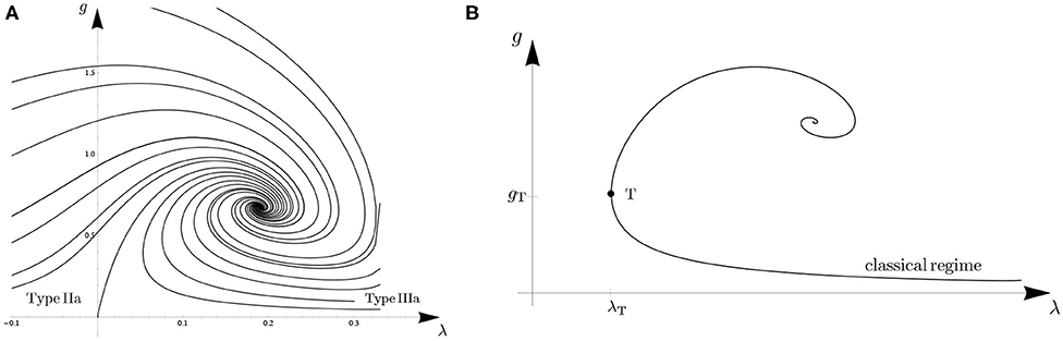
Figure 3. (A) Phase portrait of the RG flow in the Einstein-Hilbert truncation on the dimensionless (g, λ)-plane. The RG trajectories start out from the UV non-Gaussian fixed point and flow toward the IR. (B) An example of a trajectory of Type IIIa. Its turning point (λT, gT) is passed when k = kT = 1/ℓ.
There, thanks to Asymptotic Safety, the k → ∞ behavior is determined by the non-Gaussian UV fixed point, being λk → λ*, and so . In what follows, use will not be made of this specific UV completion, and many others would do as well for what concerns our main argument. It will only rely on the semiclassical formula (2.31). Despite this, the choice of trajectory, having a positive cosmological constant in the IR, Λ0, is essential.
The simple formula (2.31) should be seen as a “caricature” of a generic semiclassical behavior that is precise enough to display the crucial feature of a turning point when the trajectory is plotted on the dimensionless g − λ-plane. There,
and so λk is seen to switch from decreasing to increasing when k passes the turning point scale kT = 1/ℓ from below, see Figure 3B.
We assume that, on the one hand, kT is much smaller than the Planck scale, but, on the other, it is much larger than the Hubble parameter at k = 0:
For illustration's sake, we may fit the formula (2.31) to the values of Λ0 and G0 measured in Nature. Up to factors of order unity, this yields
with the present Hubble parameter . Both inequalities in (2.33) are well-satisfied then.
(12) The S4 family in the semiclassical regime. With Λk given by (2.31), the members of the S4 family of maximally symmetric self-consistent backgrounds have radii
where . In the strictly classical regime (k≪kT) the radius is essentially constant, , while it decreases rapidly () when k ≫ kT. As a consequence, the eigenvalues on the S4 with radius are
This spectral flow has the qualitative features anticipated in Figure 2.
The k-dependent cutoff quantum number is explicitly known at this point, with (2.30) yielding
The functions q (k) and nCOM(k) are plotted in Figure 4. They possess a maximum at the turning point scale k = kT ≡ 1/ℓ, where q (k) assumes the value
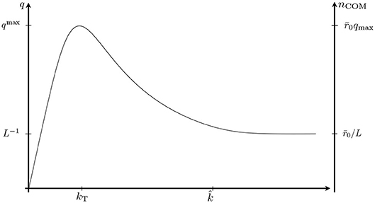
Figure 4. Representations of the functions q (k) and along a trajectory of the Type IIIa. The semiclassical regime extends from k = 0 to . Beyond this point, the Asymptotic Safety result is shown for concreteness, being q (k) = L−1 = const, with .
Under the condition (2.33), this maximum is situated well within the semiclassical regime. The value of the quantum number nCOM never can become really large. At the very least in the semiclassical domain, it is bounded above:
(13) Fuzzy appearance of spacetime. Recall that the integer n, much like the quantum number l of Ylm, measures the degree of complexity (number of nodes etc.) of the corresponding eigenfunctions. Hence nCOM(k) characterizes the maximum “resolving power” or “fineness” that can be achieved on the self-adjusting 4-sphere with an eigenfunction expansion that is truncated at n = nCOM(k).
Since nCOM(k) is bounded above by its value at the turning point, nCOM(kT), it follows that on the family of self-consistent spacetimes, whatever is the value of k, the “resolving power” of the eigenmodes is never perfect.
The best angular resolution that can be achieved on S4 is of order 2π/nCOM(kT), and this renders spacetime a kind of “fuzzy sphere.” (See also [51–53] for a discussion of a related dynamically generated minimum length, and [54] for the concomitant effect on the entanglement entropy).
(14) Anomalous mode reshuffling explained. Our usual intuition being trained on k-independent metrics, the behavior of nCOM(k) shown in Figure 4 comes as a surprise: while we expect that by increasing the characteristic momentum of the coarse graining, i.e., k, higher eigenmodes of the Laplacian with shorter wavelength get involved, the opposite happens according to Figure 4 at scales above the turning point (k > kT). Increasing k leads to a lower cutoff mode then, i.e., a function with less structure (having fewer nodes, etc.).
Another side of the same medal is that, above the turning point, lowering k converts UV-modes to IR-modes (rather than vice versa). Hence, at low scales, the effective field theory has more degrees of freedom to deal with than at high scales. This is again in conflict with the naive fixed k intuition, which would suggest that lowering k means “integrating out,” hence a relocation of modes in the opposite direction, ΥUV → ΥIR.
Thus, we observe that the spectral flow at hand, Equation (2.36), does indeed realize the possibility of eigenvalues which, in Figure 2, cross the diagonal twice.
Given the explicit form of the eigenvalues in (2.36), we can explain the above “paradoxes” in elementary physical terms:
when k is increased, the radius of the self-consistent sphere shrinks, and this causes n(k), n fixed, to grow. There are two ways of making n(k) large: the familiar one of increasing n at fixed radius and the new one of keeping n fixed, or making it smaller, while decreasing the radius. Above the turning point, this second mechanisms turns out to be the dominant one.
The analysis carried out in this section assumes a positive curvature, the extension of our investigation to the cases of negative curvature or Lorentzian signature is interesting and requires further study (Ferrero R and Reuter M, work in progress).
4. Running vs. Rigid Picture of the RG Evolution
(1) The familiar “running picture.” Assume we are given a certain solution to the functional RG equation, Γk[h, ψ; ], describing gravity coupled to a set of matter fields, ψ. Then, as for the associated effective field theory, the couplings it encapsulates apply to the “particle physics” of hμν and the other quanta when they propagate on the running geometries.
The high-k matter physics predictions supplied by Γk are valid only in conjunction with a high-k gravitational background.
This is the standard way of interpreting the RG trajectories. It refers all “particle physics” to the k-dependent on-shell geometry and is therefore called the “running picture” of the generalized RG trajectory.
(2) The novel “rigid picture” ⋯. To describe the alternative “rigid picture” let us put ourselves in the place of collider physicists who are able to measure the matter couplings governed by , but are unable to explore the microscopic spacetime structure. They would find it natural to construct a new action functional, Γq, which makes no reference to a running metric and eliminates everywhere in favor of the (essentially flat) macroscopic metric . In the sought for description only the particle physics runs, while the metric stays fixed, being always .
Among other changes of an essentially kinematic character, the construction of Γq from Γk involves re-interpreting the cutoff scale as an eigenvalue of (−□) built from rather than the usual . It is easy to see that the two operators have the same eigenfunctions and that, if the eigenvalue in the latter case is k2, then it equals q2 in the former. (Note that for metrics of the rescaling type).
In this rigid picture, therefore, the quantity q plays the same role the usual cutoff k plays in the running picture and, consequently, the notation Γq for the new running action. From the perspective of Γq, all momenta are proper with respect to the fixed metric , as desired by the collider physicists.
In order to actually construct the new action functional, we would have to reparametrize the RG time axis,
which requires inverting the function k ↦ q (k) to obtain k = k (q). This is impossible though.
In the semiclassical regime a given value q < qmax is associated to two k-values via Equation (2.37), see Figure 4. It follows that, globally speaking, the map k ↦ q (k) is not a valid reparametrization of the whole RG trajectory since it does not provide a diffeomorphism on the RG-time axis.
Locally, however, it is possible to invert Equation (2.37) for either k < kT or k > kT. The inversion yields the following two maps k = k (q) for q ∈ [0, qmax]:
The functions k+(q) and k−(q) joins at while, for a generic q, the upper branch is given by k+(q) > kT and the lower branch by k−(q) < kT.
(3) ⋯ and its breakdown. The non-invertibility of q (k) implies that the rigid picture is applicable from k = 0 up to k = kT only. It breaks down at the turning point, which acts as a sort of horizon in the one-dimensional space of scales [26].
Figure 5 illustrates the role played by this “scale horizon” in connection with the cosmological constant. The action Γq includes a term , with Λk (q) ≡ Λrigid(q) the natural scale dependent cosmological constant in the running picture. From , and with (3.2) we obtain the double-valued relation
The behavior of Λrigid is displayed in Figure 5, with the minus (plus) sign corresponding to the lower (upper) branch of the function.
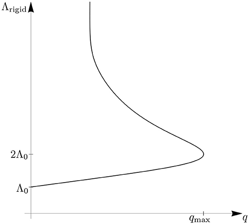
Figure 5. The cosmological constant appearing in the rigid picture's Γq in dependence on its natural RG scale q. While we are able to consistently interpret the diagram's lower branch (Λ0 ≤ Λrigid ≤ 2Λ0), the “scale horizon” at qmax prevents us from passing to the upper branch straightforwardly.
A hypothetical collider physicist that insists on using the scale q has no problems in interpreting the lower branch of Λrigid(q) but is not able to go beyond the horizon located at q = qmax.
By viewing q as a curve parameter for the RG trajectory, we note that it provides a “good” coordinate on the RG time axis only below the turning point. A different coordinate is needed to go beyond the horizon, an example is offered by k, which is valid globally. The situation is somewhat similar to the usual coordinate horizons in spacetime. In terms of q the rigid picture based on the (perturbative) k−-branch is valid for momenta q ≤ qmax.
5. Implications for Gravitating Vacuum Fluctuations and the Cosmological Constant
The cosmological constant has been puzzling physicists for a long time [55–58]. The problem involves classical and quantum aspects of both matter and gravitation. There is a general consensus that such a small cosmological constant poses an extraordinary naturalness problem. According to usual arguments the cosmological constant is unnaturally small in comparison to the vacuum energy density due to the quantum fluctuations of the quantum field theories describing particle physics. In another variant of the argument, the cosmological constant is small in relation to the Planck scale.
In this section we will focus on the former version of the “cosmological constant problem” and we shall revisit it from the perspective of Background Independent quantum field theory.
5.1. The Standard Argument
The best-known argument showing the claimed tension between quantum field theory and general relativity goes as follows. In Minkowski space, one assumes that each mode pertaining to a certain quantum field behaves like a harmonic oscillator, which contributes to the field's ground state energy by an amount . In flat space, the modes of a quantum fields are labeled by the 3-momentum p. By summing over all momenta, one obtains the total vacuum energy as . For instance, in the case of a massless free field the energy density is given by the integral
which is ultraviolet divergent and requires regularization. For instance, one may regularize the integral (4.1) via a sharp cutoff |p| ≤ . Clearly, different regularization can also be employed. In any case the vacuum energy density is quartically divergent, i.e.,
where the particular value of c depends on the chosen regularization scheme and is of order unity. Next, the UV cutoff is fixed to some high value (typically related to a new physics scale). The energy density ρvac is then taken into account in the Einstein's equation as a contribution to the cosmological constant in the amount of .
Similar semiclassical arguments goes back to Pauli [57]. He had already realized that a cosmological constant of order ΔΛ would produce a curvature, which is unacceptable even if the UV cutoff is taken to be the scale of atomic physics.
In the modern version of the argument, the UV cutoff often corresponds to the Planck scale ( = mPl). In this latter case, the contribution to the cosmological constant ΔΛ is roughly 10120 times bigger than the observed cosmological constant, Λobs. Then, by expressing the observed cosmological constant as the sum of a bare cosmological constant Λbare and ΔΛ, i.e., Λobs = Λbare + ΔΛ, one observes that Λbare must be fine tuned at the level of 120 digits. This is thus considered a major naturalness problem.
Similar issues arise with essentially any plausible choice for the UV cutoff . This has triggered the suspicion that there may be something incorrect in the previous argument. In the following we argue that this is indeed the case. Let us note that, along different lines with respect to the ones invoked in the present work, quartic divergences on a fixed Minkowski background have been shown incompatible with Lorentz symmetry [59–61].
5.2. Lessons From the Rigid Picture
Comparing the above standard argumentation to our approach we observe that
(1) The standard calculation amounts to the quantization of a free matter field's modes in ΥIR(). They constitute a low energy effective field theory with UV cutoff at . The field quantization it amounts to is equivalent to staying within the EAA framework and lowering the cutoff from down to zero.
(2) Since the calculation includes no gravitational back reaction on the Minkowski metric, it possesses a translation to the Background Independent EAA language at best if the “rigid picture” of the RG flow is invoked.
(3) The domain of applicability of the rigid picture restricts the cutoff to the interval 0 ≤ ≤ qmax below the turning point. Within this interval, the vacuum fluctuations change the cosmological constant by not more than a factor 2; according to (3.3), Λrigid(q) increases from Λrigid(0) = Λ0 to Λrigid(qmax) = 2Λ0 along the k−-branch.
It therefore follows that the traditional argument on the gravitational impact of summed up zero-point energies overstretches its domain of validity quite considerably.
We just learned that the enormous cosmological constants that are often claimed to be induced by quantum vacuum fluctuations, like , can never result from such a calculation if one restricts it to the momentum scales it is valid for, i.e., those where the rigid picture is available (q ≤ qmax). A calculation neglecting the backreaction on the metric becomes invalid already when the zero-point energies have changed the cosmological constant from Λ0 to 2Λ0.
Because no large numbers are involved in the renormalization Λ0 → 2Λ0, we can also say that it is incorrect to claim on the basis of the traditional argument that a small value of the cosmological constant is necessarily afflicted by a naturalness problem [26].
5.3. Lessons From the Running Picture
Let us now move to scales above the turning point and ask about the physical contents of the generalized RG trajectory there.
(1) Since the rigid picture is unavailable at scales k > kT, we fall back upon the running picture which applies everywhere along the trajectory. Now, the complication is that the running of the consistent background metric cannot be “transformed away” any longer and must be taken into account in explicit form.
(2) The metric is determined by the k-dependent Einstein equation (2.18). To see the essential point, its contraction is sufficient:
We are interested in the question why the rapidly increasing cosmological constant for k ≫ kT seems in no way mirrored by our cosmological observations. On the basis of the effective field theory description with Equation (4.3), the answer is as follows:
when Λk grows with increasing k beyond the experimental bounds of the observed cosmological constant Λ0 ≡ Λk = 0, the effective field theory with the Einstein equation (4.3) ascribes the associated growing curvature to much smaller, non-cosmological distance scales; the smaller they are, the larger is k. On those sub-cosmological length scales, however, we have no observational tools (yet) that could measure .
This explains why to date we have seen no manifestation of the huge values that can reach and that play a central role in the traditional discussions of the cosmological constant. [see [26] for further details, and [62] for a purely classical discussion of “hiding” the cosmological constant at small distances].
(3) Paraphrasing a well-known concise summary of classical General Relativity, it can be said that Matter at scale k tells space at scale k how to curve, and space at scale k tells matter at scale k how to move.
Modeling the gravitational effect of vacuum fluctuations by simply declaring their summed zero-point energies to be a part of the cosmological constant in an otherwise classical Einstein equation violates this principle spectacularly.
Being the coefficient of the zero-derivative term in the classical gravity action, the cosmological constant should play a role for the universe on its largest scales only. However, the traditional approach, limited by the simple two-parameter form of the Einstein-Hilbert action, cannot but package the energy and momentum of even a Planck scale fluctuation, say, into this IR-related parameter.
Clearly, this hints at the necessity of much more general actions to better describe the generation of spacetime curvature scale by scale [26].
(4) Assume we were able to measure the spacetime curvature on sub-cosmological scales, say in a terrestrial lab, and that kT is indeed in the milli-electron Volt range, as suggested by (2.34). Can we observe the scale dependence of the vacuum curvature then?
The answer is that, even then, this would be extremely difficult since has a significant k-dependence only when the Λkgμν term in the Einstein's equation dominates over the matter field's stress tensor Tμν.
As long as Tμν is k-independent, the effect we are after requires ordinary matter and its fields to be very “diluted.” The late Universe, the present epoch of cosmology, is one instance where this condition is met. It remains to be seen if there are also others.
6. Conclusion
In this paper, we advocated the general expectation that the lessons from Quantum Gravity may reach far beyond its traditional realm of small Planck mass suppressed effects and questions of UV renormalizability. We emphasized that what defines modern Quantum Gravity and makes it radically different from all present theories of particle physics is the key desideratum of Background Independence. As such unrelated to any specific scale, there is no reason a priori why it should have implications for the microscopic world only.
Indeed, we argued that it is relevant to one of the purported problems surrounding the cosmological constant, namely, the gravitational effect of quantum vacuum fluctuations. Exploiting Background Independence in an essential way we demonstrated that most of the vacuum fluctuations could not manifest themselves in the cosmological constant Λ measured at cosmological scales since such fluctuations affect the curvature of spacetime only at sub-cosmological scales.
In principle, a mechanism of this sort could resolve the conundrum regarding the invisibility of spacetime curvature due to quantum vacuum fluctuations and the associated energy density, which is possibly the most mysterious facet of the cosmological constant problem.
From the perspective adopted in this work, our analysis shows no tension or “clash” between theoretical expectations and actual observations.
Data Availability Statement
The original contributions presented in the study are included in the article/supplementary materials, further inquiries can be directed to the corresponding author/s.
Author Contributions
All authors listed have made a substantial, direct and intellectual contribution to the work, and approved it for publication.
Conflict of Interest
The authors declare that the research was conducted in the absence of any commercial or financial relationships that could be construed as a potential conflict of interest.
Footnotes
1. ^More general composite operators O (μν) can be included in the gravitational EAA [34–38] by coupling them to independent sources [39–45].
2. ^Alongside with h = 0 we also fix other fluctuation fields in the multiplet φ = (h, ⋯), e.g., the ghosts and matter fields, according to their solution from the coupled field or tadpole equations.
References
1. Ashtekar A, Reuter M, Rovelli C. From general relativity to quantum gravity. In: Ashtekar A, Berger BK, Isenberg J, MacCallum M, editors. General Relativity and Gravitation: A Centennial Perspective. Cambridge, UK: Cambridge University Press (2015). Available online at: https://www.cambridge.org/core/books/general-relativity-and-gravitation/57AFB47FCEB825B190CAB4ABD04BB297
2. Reuter M. Nonperturbative evolution equation for quantum gravity. Phys Rev D. (1998) 57:971. doi: 10.1103/PhysRevD.57.971
3. Weinberg S. Ultraviolet divergences in quantum theories of gravitation. In: Hawking SW, Israel W, editors. General Relativity: An Einstein Centenary Survey. Cambridge, MA: Cambridge University Press (1979). p. 790–831.
5. Reuter M, Saueressig F. Renormalization group flow of quantum gravity in the Einstein-Hilbert truncation. Phys Rev D. (2002) 65:065016. doi: 10.1103/PhysRevD.65.065016
6. Lauscher O, Reuter M. Ultraviolet fixed point and generalized flow equation of quantum gravity. Phys Rev D. (2002) 65:025013. doi: 10.1103/PhysRevD.65.025013
7. Lauscher O, Reuter M. Is quantum Einstein gravity nonperturbatively renormalizable? Class Quant Grav. (2002) 19:483–92. doi: 10.1088/0264-9381/19/3/304
8. Lauscher O, Reuter M. Flow equation of quantum Einstein gravity in a higher derivative truncation. Phys Rev D. (2002) 66:025026. doi: 10.1103/PhysRevD.66.025026
9. Reuter M, Saueressig F. Quantum Gravity and the Functional Renormalization Group – The road towards Asymptotic Safety. Cambridge UK: Cambridge University Press (2019).
10. Percacci R. An Introduction to Covariant Quantum Gravity and Asymptotic Safety. Singapore: World Scientific (2017).
11. Gies H, Knorr B, Lippoldt S, Saueressig F. Gravitational two-loop counterterm is asymptotically safe. Phys Rev Lett. (2016) 116:211302. doi: 10.1103/PhysRevLett.116.211302
12. Knorr B, Lippoldt S. Correlation functions on a curved background. Phys Rev D. (2017) 96:065020. doi: 10.1103/PhysRevD.96.065020
13. Gonzalez-Martin S, Morris TR, Slade ZH. Asymptotic solutions in asymptotic safety. Phys Rev D. (2017) 95:106010. doi: 10.1103/PhysRevD.95.106010
14. Eichhorn A, Labus P, Pawlowski JM, Reichert M. Effective universality in quantum gravity. SciPost Phys. (2018) 5:031. doi: 10.21468/SciPostPhys.5.4.031
15. De Brito GP, Ohta N, Pereira AD, Tomaz AA, Yamada M. Asymptotic safety and field parametrization dependence in the f (R) truncation. Phys Rev D. (2018) 98:026027. doi: 10.1103/PhysRevD.98.026027
16. Falls KG, Litim DF, Schröder J. Aspects of asymptotic safety for quantum gravity. arXiv [Preprint]. arXiv:1810.08550. doi: 10.1103/PhysRevD.99.126015
17. Manrique E, Reuter M. Bimetric truncations for quantum Einstein gravity and asymptotic safety. Ann Phys. (2010) 325:785. doi: 10.1016/j.aop.2009.11.009
18. Manrique E, Reuter M, Saueressig F. Matter induced bimetric actions for gravity. Ann Phys. (2011) 326:440–62. doi: 10.1016/j.aop.2010.11.003
19. Manrique E, Reuter M, Saueressig F. Bimetric renormalization group flows in quantum Einstein gravity. Ann Phys. (2011) 326:463–85. doi: 10.1016/j.aop.2010.11.006
20. Becker D, Reuter M. En route to background independence: broken split-symmetry, and how to restore it with bi-metric average actions. Ann Phys. (2014) 350:225–301. doi: 10.1016/j.aop.2014.07.023
21. Percacci R, Perini D. Constraints on matter from asymptotic safety. Phys Rev D. (2003) 67:081503. doi: 10.1103/PhysRevD.67.081503
22. Donà P, Eichhorn A, Percacci R. Matter matters in asymptotically safe quantum gravity. Phys Rev D. (2014) 89:084035. doi: 10.1103/PhysRevD.89.084035
23. Christiansen N, Litim DF, Pawlowski JM, Reichert M. Asymptotic safety of gravity with matter. Phys Rev D. (2018) 97:106012. doi: 10.1103/PhysRevD.97.106012
24. Alkofer N, Saueressig F. Asymptotically safe f (R)-gravity coupled to matter I: the polynomial case. Ann Phys. (2018) 396:173–203. doi: 10.1016/j.aop.2018.07.017
25. Eichhorn A. An asymptotically safe guide to quantum gravity and matter. arXiv [Preprint]. arXiv:1810.07615. doi: 10.3389/fspas.2018.00047
26. Pagani C, Reuter M. Background independent quantum field theory and gravitating vacuum fluctuations. Ann Phys. (2019) 411:167972. doi: 10.1016/j.aop.2019.167972
27. Reuter M, Wetterich C. Average action for the Higgs model with Abelian gauge symmetry. Nucl Phys B. (1993) 391:147–75. doi: 10.1016/0550-3213(93)90145-F
28. Reuter M, Wetterich C. Running gauge coupling in three-dimensions and the electroweak phase transition. Nucl Phys B. (1993) 408:91–130. doi: 10.1016/0550-3213(93)90134-B
29. Wetterich C. Exact evolution equation for the effective potential. Phys Lett B. (1993) 301:90–4. doi: 10.1016/0370-2693(93)90726-X
30. Reuter M, Wetterich C. Effective average action for gauge theories and exact evolution equations. Nucl Phys B. (1994) 417:181–214.
31. Reuter M, Wetterich C. Exact evolution equation for scalar electrodynamics. Nucl Phys B. (1994) 427:291–324. doi: 10.1016/0550-3213(94)90278-X
33. Morris TR. The Exact renormalization group and approximate solutions. Int J Mod Phys A. (1994) 9:2411–50.
34. Pagani C, Reuter M. Composite operators in asymptotic safety. Phys Rev D. (2017) 95:066002. doi: 10.1103/PhysRevD.95.066002
35. Becker M, Pagani C. Geometric operators in the asymptotic safety scenario for quantum gravity. Phys Rev D. (2019) 99:066002. doi: 10.1103/PhysRevD.99.066002
36. Becker M, Pagani C. Geometric operators in the Einstein–Hilbert truncation. Universe. (2019) 5:75. doi: 10.3390/universe5030075
37. Becker M, Pagani C, Zanusso O. Fractal geometry of higher derivative gravity. arXiv [Preprint]. arXiv:1911.02415. doi: 10.1103/PhysRevLett.124.151302
38. Houthoff W, Kurov A, Saueressig F. On the scaling of composite operators in asymptotic safety. arXiv [Preprint]. arXiv:2002.00256. doi: 10.1007/JHEP04(2020)099
39. Pawlowski JM. Aspects of the functional renormalisation group. Ann Phys. (2007) 322:2831–915. doi: 10.1016/j.aop.2007.01.007
40. Igarashi Y, Itoh K, Sonoda H. Realization of symmetry in the ERG approach to quantum field theory. Prog Theor Phys Suppl. (2010) 181:1. doi: 10.1143/PTPS.181.1
41. Pagani C. Note on scaling arguments in the effective average action formalism. Phys Rev D. (2016) 94:045001. doi: 10.1103/PhysRevD.94.045001
42. Pagani C, Sonoda H. Products of composite operators in the exact renormalization group formalism. Prog Theor Exp Phys. (2018) 2018:023B02. doi: 10.1093/ptep/ptx189
43. Pagani C, Sonoda H. Geometry of the theory space in the exact renormalization group formalism. Phys Rev D. (2018) 97:025015. doi: 10.1103/PhysRevD.97.025015
44. Pagani C. Functional renormalization group approach to the Kraichnan model. Phys Rev E. (2015) 92:033016. doi: 10.1103/PhysRevE.92.033016
45. Pagani C, Sonoda H. Operator product expansion coefficients in the exact renormalization group formalism. arXiv [Preprint]. arXiv:2001.07015. doi: 10.1103/PhysRevD.101.105007
46. Lippoldt S. Renormalized functional renormalization group. Phys Lett B. (2018) 782:275–9. doi: 10.1016/j.physletb.2018.05.037
47. Pilch K, Schellekens AN. Formulae for the Eigenvalues of the Laplacian on tensor harmonics on symmetric coset spaces. J Math Phys. (1984) 25:3455. doi: 10.1063/1.526101
48. Rubin MA, Ordonez CR. Symmetric tensor Eigen spectrum of the Laplacian on n spheres. J Math Phys. (1984) 25:2888.
49. Rubin MA, Ordonez CR. Symmetric tensor Eigen spectrum of the Laplacian on n spheres. J Math Phys. (1985) 26:65. doi: 10.1063/1.526749
50. Higuchi A. Symmetric tensor spherical harmonics on the N sphere and their application to the De Sitter group SO(N,1). J Math Phys. (1987) 28:1553.
51. Reuter M, Schwindt JM. A Minimal length from the cutoff modes in asymptotically safe quantum gravity. J High Energy Phys. (2006) 0601:070. doi: 10.1088/1126-6708/2006/01/070
52. Reuter M, Schwindt JM. Scale dependent metric and minimal length in QEG. J Phys A. (2007) 40:6595. doi: 10.1088/1751-8113/40/25/S04
53. Reuter M, Schwindt JM. Scale-dependent metric and causal structures in Quantum Einstein Gravity. J High Energy Phys. (2007) 0701:049. doi: 10.1088/1126-6708/2007/01/049
54. Pagani C, Reuter M. Finite entanglement entropy in asymptotically safe quantum gravity. J High Energy Phys. (2018) 1807:039. doi: 10.1007/JHEP07(2018)039
57. Straumann N. The mystery of the cosmic vacuum energy density and the accelerated expansion of the universe. Eur J Phys. (1999) 20:419. doi: 10.1088/0143-0807/20/6/307
58. Straumann N. The history of the cosmological constant problem. arXiv [Preprint]. arXiv:gr-qc/0208027.
59. Ossola G, Sirlin A. Considerations concerning the contributions of fundamental particles to the vacuum energy density. Eur Phys J C. (2003) 31:165–75. doi: 10.1140/epjc/s2003-01337-7
61. Vacca G, Zambelli L. Functional RG flow equation: regularization and coarse-graining in phase space. Phys Rev D. (2011) 83:125024. doi: 10.1103/PhysRevD.83.125024
Keywords: asymptotic safety, background independent quantum gravity, renormalization group, cosmological constant, functional renormalization group
Citation: Pagani C and Reuter M (2020) Why the Cosmological Constant Seems to Hardly Care About Quantum Vacuum Fluctuations: Surprises From Background Independent Coarse Graining. Front. Phys. 8:214. doi: 10.3389/fphy.2020.00214
Received: 11 March 2020; Accepted: 20 May 2020;
Published: 13 August 2020.
Edited by:
Antonio D. Pereira, Universidade Federal Fluminense, BrazilReviewed by:
Luca Zambelli, Real Jardín Botánico (RJB), SpainJulien Serreau, Université de Paris, France
Copyright © 2020 Pagani and Reuter. This is an open-access article distributed under the terms of the Creative Commons Attribution License (CC BY). The use, distribution or reproduction in other forums is permitted, provided the original author(s) and the copyright owner(s) are credited and that the original publication in this journal is cited, in accordance with accepted academic practice. No use, distribution or reproduction is permitted which does not comply with these terms.
*Correspondence: Carlo Pagani, Y2FybG8ucGFnYW5pQGxwbW1jLmNucnMuZnI=