Research on Dynamic Evolution of Systemic Risk in Chinese Banking System

Systemic risk is not only related to the contagious risk of interbank market risk exposure, but also to the credit risk exposure. At the same time, the dynamic characteristics of banking system also affect the systemic risk. A large number of studies have revealed the contagious risk of interbank market risk exposure, but the systematic risk research that considers these factors at the same time is still rare. Therefore, the present paper constructs dynamically evolving banking systemic risk assessment model under double risk exposures in the same framework that includes two parts: one is the assessment of credit risk; the other is the contagious risk. On the assessment of credit risk, we use Geometric Brownian Motion in physics and Monte Carlo simulation calculation method based on the big data of the stock market. On the assessment of contagious risk, we use the method of Geometric Brownian Motion in physics and minimum density method. Then we use data of 205 Banks and 3,017 listed companies in 18 industries in Chinese to study the dynamic evolution law of the Chinese banking systemic risk. The results show that the evolution characteristics of credit risk of 18 real industries can be divided into 4 types which are stability after decline, increase in fluctuation, decrease in fluctuation, and fluctuation. The systemic risk of Chinese banking system with the double risk exposures gradually increased with the evolution of time, and then stabilized at a certain degree. Among them, the initial increase of contagious risk is fast, and then stable; the credit risk starts small, slowly increases, and eventually stabilizes. The evolution degree of contagious risk is higher than that of credit risk. Large banks have the strongest ability to withstand the impact of double risk exposures, while foreign banks have the weakest.

Introduction

After the international financial crisis in 2008 and the European debt crisis in 2010, countries have paid enough attention to strengthening financial supervision, maintaining financial stability, and preventing and controlling systemic risks. In October 2017, the report of the 19th National Congress of the Communist Party of China clearly pointed out that it is necessary to “improve the financial supervision system, keep the bottom line of no systemic financial risks,” and raised the prevention of systemic risk to the height of national security. However, due to the complexity of systemic risk itself, the definition of systemic risk has not been unified in academia. But, some studies have clearly pointed out that systemic risk is a global and systematic risk, which is not limited to the financial system. It is worth noting that the real industry plays a more and more important role in the process of economic development, and the relationship between the real industry and the financial industry is increasingly close. These correlations not only constitute the channel of risk transmission, but also further expand the negative impact on the entire economic system. When the important real industries encounter difficulties, the contagion risk brought by the recession makes our economy face great risks.

In financial system, the banking industry plays an important role. To prevent the systemic risk of the banking industry has become the core of maintaining financial stability. At present, the systemic risk is mainly studied on the contagious risk of interbank market risk exposure, while there are few studies on the double risk exposures of basic failure caused by credit risk exposure and contagious risk caused by interbank market risk exposure.

Since Allen and Gale [1] used the network model to study the impact of the interbank network structure on the banking systemic risk, the research on the banking systemic risk has been emerging. The mutual loan relationship between banks can solve the short-term liquidity shortage of banks and increase investment opportunities, but it can also improve the contagion risk between banks. Most researches show that the risk exposure of interbank market is the main channel of systemic risk. Allen and Gale [1] found that the fully connected network structure is more robust than the incomplete network structure, and the contagion risk is significantly smaller. Freixas et al. [2] found the probability of contagion risk depends on the setting of network model parameters by comparing the fully connected network structure with the ring network structure. Using the data of 27 Mexican banks in 2007, Martínez-Jaramillo [3] found that the vulnerability of the banking system is determined by the probability of banks default, the connectivity between banks, and the banks that are over exposed to the network. Mistrulli [4] found that the fully connected interbank market is more susceptible to contagion than the incompletely connected interbank market. Ladley [5] found that there is no interbank market structure that can maximize the stability under any conditions. Sui et al. [6] studied the problem of contagion risk in scale-free networks with different scale parameters and found that the higher the concentration, the more the number of banks in the network with contagion failure. Bao and Sun [7] studied financial structure and contagion risk by establishing a multi-agent simulation model and found that the hierarchical structure of center edge will increase the degree and scope of contagion risk compared with the fully connected structure.

Although the interbank market risk exposure is the core of the study of banking systemic risk, the impact of credit risk exposure on the systemic risk of banks cannot be ignored. At present, there are few studies on credit risk exposure based on VaR-based method, while those researches did not consider the effect of the interbank market risk exposure on systemic risk. In the existing literature, Adrian and Brunnermeier [8] proposed a CoVaR to measure the contribution of financial institution to the systemic risk. Huang et al. [9] measured the systemic risk as the marginal contribution of a financial firm to the distress insurance premium of the financial sector. A large number of contributions on VaR-based systemic risk measurement associate the systemic risk with the degree of interdependence among financial firms as in Billio et al. [10], Ang and Longstaff [11], and Diebold and Yilmaz [12]. In China, Li et al. [13] used 11 industry VaR indexes to build the systemic risk spillover network among industries in China from 2002 to 2017 to find that the financial industry is not the only systemic risk source and the systemic importance of information technology, materials, industry, and other real economic industries is increasing day by day. Zhai [14] established GARCH-Copula-CoVaR model based on industry indexes to empirically analyze the two-way risk spillover effect between each real industry and banking industry. Zhu and Ma [15] used the method of eigenvector centrality to measure the systemic risk of China's industry and found that the systemic risk of the financial industry is generally on the decline, while the systemic risk of the non-financial industry is at a relatively high level. Sun et al. [16] used the real estate industry index to measure the systemic risk spillover intensity of China's real estate industry to the financial industry based on the CoVaR model and quantile regression method.

Based on the perspective of complex network, few studies consider credit risk exposure and interbank market risk exposure at the same time; most of them are theoretical studies and lack of empirical data support. In addition, the systemic risk of those studies is mainly based on the static model without considering the evolution of the systemic risk over time. Lu and Wang [17] used the maximum entropy method to estimate the complete interbank network and set up a common loan network of banks based on the covariance of industry indexes, but they did not consider the credit risk of industry default and the evolution of the systemic risk over time. In their study, they found that the impact of different loan industry shocks on the degree of contagion risk is different. The crisis in the industry with more loan funds is more serious for the financial system. Wu et al. [18] studied theoretically the impact of the price fluctuation of common assets on the systemic risk and found that the indirect linked contagion of the sale of common assets is far greater than the direct linked contagion. Although this study involves credit risk exposure, the systematic risk in this study is based on the assumption of the model, not supported by the actual data, and the model of the credit risk exposure is static. Zhai and Bian [19] used the maximum entropy estimation method to construct the interbank network structure and the bipartite network structure between banks and real industries to identify the systemic important bank and the systemic important industry, but they did not study the effect of credit risk on the systemic risk. Caccioli et al. [20] found theoretically that interbank market risk exposure magnified the chain reaction of bank portfolio risk exposure. Glasserman and Young [21] also found theoretically that the probability of bank default caused by the direct impact of external asset loss is higher than that of bank contagion default, and the interconnected financial network can increase the expected loss and default degree. Chiu et al. [22] found that there is a relationship between creditor's rights and debts between the real industry and the banking industry and the risk will circulate among different departments. In addition, the systemic risk should be discussed from the perspective of the whole industry. The banking industry and the real industry are closely linked through credit. Wang and Li [23] established an extended matrix model based on the credit market between the banking and real estate industry. They found that the financial system composed of the real estate industry and the banking industry is more vulnerable than the separate banking system and the risk transmission speed is significantly faster. Li et al. [24] studied the joint impact of Chinese Banks' internal lending market and real estate industry's credit risk exposure on the systemic risk of the banking system and found that the two had a great joint resonance effect on contagion risk. The study only considered real estate credit risk exposure, instead of all the industries.

To sum up, at present, most of the researches on credit risk exposure use VaR-based method to study the impact of credit risk spillover on systemic risk without considering the interbank market risk exposure, and these studies only qualitatively point out the importance of credit risk exposure of the real industry for the assessment of systemic risk and do not quantitatively analyze the default probability of the real industry and the quantitative effect of credit risk on systemic risk. Few studies consider both credit risk exposure and the interbank market risk exposure; however, most of them are theoretical studies and lack of empirical data support; in addition, the systematic risk of those studies is mainly based on the static model without considering the evolution of systemic risk over time. Therefore, the present paper studies the dynamical evolution of systemic risk in the same framework of both the credit risk exposure of the real industry and the contagion risk exposure of the interbank market. In order to construct the dynamical evolution of the systemic risk, the present paper uses the Geometric Brownian Motion to simulate the movement of assets of the real industry and banks, which is often used to estimate the dynamic motion of assets in economics [25, 26]. In Lehar [25], Lehar first used the Geometric Brownian Motion to simulate the movement of assets of banks and studied the systemic risk based on the correlation of assets of banks, but the study did not consider the interbank market and the real industry that banks loan to. After constructing the dynamic evolution of assets and liabilities, the present paper uses the simulation methods, complex network methods, and empirical data to build a dynamic evolution model of banking systemic risk assessment to analyze the impact of the direct shock of credit risk exposure of the real industry and the indirect shock of interbank market exposure on the systemic risk of China's banking system.

The innovation of this paper is mainly in three aspects. First, inspired by the research of Caccioli et al. [20] and Lehar [25], the present paper is the first to combine the credit risk exposure of the real industry and the risk exposure of the interbank lending market in the same framework to conduct the dynamic evolution study of systemic risk by using Geometric Brownian Motion in physics. Second, consider that most of studies used the maximum entropy method to estimate the interbank network and lacked real data support, the present paper uses real data of listed companies in the real industry to estimate the dynamic credit risk exposure of real industry, then uses the minimum density method and real banking data to estimate the more realistic dynamic interbank market risk exposure. Third, in the existing literature, the method of stress test for banks is to let one or one type of bank assets lose, while in this paper, the listed companies in the real industry are shocked, which causes those companies bankruptcy, thus the credit risk of the real industry is formed.

This paper is organized as follows. In section Model, we describe the dynamic evolution model of banking systemic risk assessment under double risk exposures. In section The Calculation of Banking Systemic Risk Under Double Risk Exposures, we propose how to calculate the systemic risk of the banking system. In section Data, we explain the source of data. In section Results, we discuss the assessment of dynamically evolving banking systemic risk under double risk exposures which include two parts: one is the assessment of credit risk of the real industry in section The Assessment of Credit Risk of the Real Industry; the other is the contagious risk section The Assessment of Systemic Risk under Double Risk Exposures. In section Discussion and Conclusions, we give conclusions.

Model

In this section, we first build a dynamic evolution model of banking systemic risk assessment under double risk exposures, as shown in Figure 1. We assume that there are a set N = {1, ⋯N} of banks in the system, each bank has a dynamically evolved bank balance sheet structure as shown in Figure 1A. Each bank's assets include interbank lending assets A_i(t) and external assets V_i(t). Each bank's liabilities include interbank borrowing liabilities L_i(t) and external liabilities D_i(t). Each bank's assets minus liabilities is owner's equity e_i(t). The double risk exposures faced by banks refer to the credit risk exposure of the real industry shown in Figure 1B and the interbank market risk exposure shown in Figure 1C (The payment matrix of the interbank market risk exposure can be described as Equation (16), which shows the interbank loan assets A_i(t)and the interbank loan liabilitiesL_i(t).). At time step T, the dynamic evolution of the credit risk exposure of the real industry (see Figure 1B) results in dynamic external asset losses for the banks (see the dashed boxes Loss_i(t) and Loss_j(t) in Figure 1A). The interbank loan assets A_i(t) and interbank loan liabilities L_i(t) are dynamic, so the interbank market risk exposure is also dynamically evolving. As shown in Figure 1D, the dynamic interbank market network structure evolved from time step t₁ to time step t₁₅₀. At each time step, we use the clearing payment vector to conduct asset and liability liquidation on the banking system under double risk exposures and to calculate the systemic risk of the banking system at each time step.

FIGURE 1

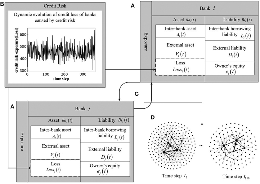
Figure 1. A dynamic evolution model of bank systemic risk assessment under double risk exposures. (A) Represents dynamic evolution of bank balance sheet structure of bank i and j. (B) Plots the dynamic evolution curve of credit loss of banks caused by credit risk of the real industry. (C) Represents interbank market risk exposure. (D) Shows dynamic evolution of interbank market network structure from time step t₁ to time step t₁₅₀.

Next, this paper constructs a dynamic evolution of credit risk exposure of the real industry corresponding to Figure 1B in section Dynamic Evolution of Credit Risk Exposure of the Real Industry and Estimation of the Interbank Market Risk Exposure constructs an interbank market risk exposure estimation model corresponding to Figure 1C. Section Default Algorithms Based on the Dynamic Evolution of Bank Balance Sheet Structure explains the default algorithms based on dynamic evolution of bank balance sheet structure corresponding to Figure 1A. Section The Dynamic Evolution of Interbank Market Network discusses the dynamic evolution of interbank market network corresponding to Figure 1D.

Dynamic Evolution of Credit Risk Exposure of the Real Industry

The credit relationship between banks and the real industry constitutes a bank-real industry credit network. When credit default occurs in the real industry, it will cause loss of external assets of the related banks. Therefore, credit risk exposure of the real industry faced by banks includes three parts that are credit network between banks and the real industry, the distribution of credit default probability in the real industry, and loss of banks' external assets caused by credit risk exposure.

Credit Network Between Banks and Real Industry

Assuming that there is m real industries in China, the loan that bank i provide to the real industry are expressed as L_ik, the assets of bank i is V_i, the proportion of loans L_ik provided by bank i to the real industry k in the assets V_i of bank i is called loan proportion, expressed as R_ik.

$\begin{array}{ll}{R}_{ik}=\frac{L_{ik}}{V_i}i=1,2,\cdots ,N,k=1,2,\cdots ,m& (1)\end{array}$

Considering that the distribution data of loan that a bank provides to the real industry is not disclosed in the annual report, it is impossible to calculate the loan proportion of all banks. Therefore, R_ikindicates the loan proportion provided by the banks that can obtain the data to the real industry.

In order to determine the loan proportion of all banks, we have divided N banks into a types, with Z banks under each type. Assuming that banks of the same type have the same loan proportion, Nbanks all provide loans to m real industries. R_bik is used to represent the proportion of loans provided by bank i under type b to real industry k. The calculation formula is as follows.

$\begin{array}{ll}{R}_{bik}=\frac{\sum R_{ik}}{Z_b}b=1,2,\cdots ,a& (2)\end{array}$

∑R_ik is the sum of Equation (1) and Z_b indicates the number of banks under type b. In the end, we calculate the proportion of loans R provided by N banks to m industries is a matrix of N × m.

$\begin{array}{cc}R=\left[\begin{array}{ccccc}{R}_{111}& \cdots & R_{11k}& \cdots & R_{11m}\\ ⋮& \ddots & ⋮& & ⋮\\ R_{bi1}& \cdots & R_{bik}& \cdots & R_{bim}\\ ⋮& & ⋮& \ddots & ⋮\\ R_{aN1}& \cdots & R_{aNk}& \cdots & R_{aNm}\\ \end{array}\right]& (3)\end{array}$

This paper assumes that every bank provides loans to every industry, then credit network Z between banks and real industry can be expressed as a matrix of N × m.

$\begin{array}{cc}Z=\left[\begin{array}{ccccc}{V}_1{R}_{111}& \cdots & V_1{R}_{11k}& \cdots & V_1{R}_{11m}\\ ⋮& \ddots & ⋮& & ⋮\\ V_i{R}_{bi1}& \cdots & V_i{R}_{bik}& \cdots & V_i{R}_{bim}\\ ⋮& & ⋮& \ddots & ⋮\\ V_N{R}_{aN1}& \cdots & V_N{R}_{aNk}& \cdots & V_N{R}_{aNm}\\ \end{array}\right]& (4)\end{array}$

Probability Distribution of Credit Default in Real Industry

Estimation of dynamic evolution of assets and liabilities of listed company in the real industry

Supposing the asset value V_g of the Listed Company in the real industryg obeys Geometric Brownian Motion in physics [25], its drift rate is μ_gand volatility is σ_g.

$\begin{array}{ll}d{V}_g={\mu }_g{V}_{g}dt+{\sigma }_g{V}_{g}dz& (5)\end{array}$

The owner's equity E_g(t) of Listed Company g is regarded as call option, whose value is equal to the nominal value of liabilities D_g(t) of Listed Company g in mature period T. Based on Black Scholes Model [26], we can obtain the relationship between owner's equity and asset value of Listed Company as Equation (6).

$\begin{array}{ll}{E}_g(t)=V_g(t)N(d_t)-D_g(t)N(d_t-{\sigma }_g\sqrt{T})& (6)\end{array}$

$\begin{array}{ll}{d}_t=\frac{ln\left(V_g(t)/D_g(t)\right)+\left({\sigma }_g^2/2\right)T}{{\sigma }_g\sqrt{T}}& (7)\end{array}$

$\begin{array}{ll}{D}_g(t)=D_g(0)e^{rt}& (8)\end{array}$

Where T is the maturity andT = 365; t is the day before maturity. E_g(t) is the daily equity value of Listed Company g, which can be obtained from the stock market. D_g(0) is the initial liability value of Listed Company g, which can be obtained from the balance sheet. This paper assumes that the liabilities of all listed companies increase according to the risk-free rate of return r.

In this paper, we first set the initial drift rate μ_g(0) and volatility σ_g(0) as any value, then get the initial asset value V_g(0) from the balance sheet of the Listed Company and the owner's equity value of each day can be expressed as E_g(0), E_g(1), ⋯ , E_g(T). According to Equation (8), the liability can be expressed as D_g(0), D_g(1), ⋯ , D_g(T), then we estimate the asset value of each day as $\stackrel{\wedge }{V_g}(0),\stackrel{\wedge }{V_g}(1),\cdots ,\stackrel{\wedge }{V_g}(T)$ according to Equations (6–8). Using the maximum likelihood function proposed by Duan J-C [27] to calculate the parameter of drift rate μ_g and volatility σ_g.

$\begin{array}{l}L\left({\mu }_g,{\sigma }_g;\stackrel{\wedge }{V_g}(0),\stackrel{\wedge }{V_g}(1),\cdots ,\stackrel{\wedge }{V_g}(T)\right)=-\frac{T}{2}ln(2\pi {\sigma }_g^{2}h)\\ -\frac{T}{2}{\displaystyle \sum _{k=1}^T}\frac{{\left({R^{*}}_g(k^{*})-({\mu }_g-\frac{{\sigma }_g^2}{2})h\right)}^2}{{\sigma }_g^{2}h}-{\displaystyle \sum _{k=1}^T}ln{\stackrel{\wedge }{V}}_t& (9)\end{array}$

In Equation (9), ${R^{*}}_g\left(k^{*}\right)=ln({\stackrel{\wedge }{V}}_g(t)/{\stackrel{\wedge }{V}}_g(t-1))$, $h=\frac{1}{365}$.

Finally, the drift rate μ_g and volatility σ_g estimated by Equation (9) are substituted into Equation (10) to estimate the assets of listed companies V_g(t).

$\begin{array}{ll}{V}_g(t)=V_g(0)e^{{\mu }_g-\left({\sigma }_g^2/2\right)th+{\sigma }_g\sqrt{th*z_g(t)}}& (10)\end{array}$

In Equation (10), z_g(t)obeys the standard distribution of N(0, 1), h = 1/T.

Calculation of basic bankruptcy status of listed companies in real industry

Basic bankruptcy occurs when assets of listed companies in various industries are less than liabilities, which can be expressed by Equation (11).

$\begin{array}{ll}{V}_g(t)-D_g(t)<0& (11)\end{array}$

In Equation (11), the assets V_g(t) and liabilities D_g(t) of listed companies have estimated in section Estimation of Dynamic Evolution of Assets and Liabilities of Listed Company in the Real Industry.

In this paper, the basic failure state variable is defined as integer of 0 or 1, which can be expressed by Equation (12):

$\begin{array}{ll}{S}_g(t)=\{\begin{array}{c}1\\ 0\end{array}\begin{array}{c}if{V}_g(t)-D_g(t)<0\\ otherwise\end{array}& (12)\end{array}$

Calculation of probability distribution of default in real industry

The number of listed companies in the industry k can be expressed as n_k.By using Monte Carlo simulation method, we calculate S_g(t) according to Equation (12), then we calculate the default probability of industry k at time step t. This paper defines the default probability of industry as Equation (13).

$\begin{array}{ll}{P}_k(t)=\frac{\sum S_g(t)}{n_k},k=1,2,\dots ,m& (13)\end{array}$

In Equation (13), P_k(t) is the default probability of industry k at time step t, ∑S_g(t) is the sum of the number of all the failed listed companies in the industry k at time step t. In this paper, P_k(t) that is the default probability curve with time changes is used to measure the evolution of credit default probability of the real industry.

Loss of Bank's External Assets Caused by Credit Risk Exposure

When listed companies in the real industry are unable to repay banks' loans in case of insolvency, the banks will suffer external asset losses due to the credit default of real industry. The loss of external assets of a bank can be calculated by combining Equation (1) and (13), which is expressed by Equation (14).

$\begin{array}{ll}Los{s}_{ik}(t)=R_{bik}\times V_i(t)\times P_{\text{k}}(t)& (14)\end{array}$

In Equation (14), Loss_ik(t) is the loss of external asset loans from bank i provides to the real industry k at time step t, V_i(t) is the asset value of bank i at time step t.

Finally, we combine the credit network between banks and real industry, the evolution sequence of bank's assets V_i, and the distribution of bank's loss of external assets Loss_ik(t) to calculate the dynamic evolution of credit risk exposure between banks and the real industry, which can be expressed by Equation (15).

$\begin{array}{ll}Loss(t)=\left[\begin{array}{ccccc}{V}_1(t)R_{111}& \cdots & V_1(t)R_{11k}& \cdots & V_1(t)R_{11m}\\ ⋮& \ddots & ⋮& & ⋮\\ V_i(t)R_{bi1}& \cdots & V_i(t)R_{bik}& \cdots & V_i(t)R_{bim}\\ ⋮& & ⋮& \ddots & ⋮\\ V_N(t)R_{aN1}& \cdots & V_N(t)R_{aNk}& \cdots & V_N(t)R_{aNm}\\ \end{array}\right]\times \left[\begin{array}{c}{P}_{\text{1}}(t)\\ ⋮\\ P_k(t)\\ ⋮\\ P_N(t)\\ \end{array}\right]& (15)\end{array}$

Estimation of the Interbank Market Risk Exposure

Considering an interbank lending network formed by N banks, this network can be expressed in N × N matrix form by Equation (16).

$\begin{array}{l}X=\left[\begin{array}{ccccc}{x}_{11}& \cdots & x_{1j}& \cdots & x_{1N}\\ ⋮& \ddots & ⋮& & ⋮\\ x_{i1}& \cdots & x_{ij}& \cdots & x_{iN}\\ ⋮& & ⋮& \ddots & ⋮\\ x_{N1}& \cdots & x_{Nj}& \cdots & x_{NN}\\ \end{array}\right]\begin{array}{c}{A}_1\\ ⋮\\ A_i\\ ⋮\\ A_N\\ \end{array}\\ \begin{array}{lllll}{L}_1& \cdots & L_j& \cdots & \\ \end{array}{L}_N& (16)\end{array}$

In the interbank lending market, x_ij refers to the loans borrowed by bankj from bank i; the sum of each row in the matrix A_i represents the total lending assets of bank i; the sum of each column in the matrix L_j represents the total lending liabilities of bank i. Since a bank itself has no lending relationship, the matrix in Equation (16) is modified to a new interbank lending network matrix with diagonal 0, which is expressed as X^* by Equation (17).

$\begin{array}{l}{X}^{*}=\left[\begin{array}{ccccc}0& \cdots & x_{1j}& \cdots & x_{1N}\\ ⋮& \ddots & ⋮& & ⋮\\ x_{i1}& \cdots & 0& \cdots & x_{iN}\\ ⋮& & ⋮& \ddots & ⋮\\ x_{N1}& \cdots & x_{Nj}& \cdots & 0\\ \end{array}\right]\begin{array}{c}{A}_1\\ ⋮\\ A_i\\ ⋮\\ A_N\\ \end{array}\\ \begin{array}{lllll}{L}_1& \cdots & L_j& \cdots & \\ \end{array}{L}_N& (17)\end{array}$

In this paper, we use the minimum density method proposed by Anand et al. [28] to estimate the interbank market risk exposure matrix X^*.

In the minimum density method, parameter c is introduced, which represents the fixed cost of establishing connection between banks, that is, if there is a connection between banks, there will be a connection cost of c, then the minimum density method can be expressed as a constraint optimization problem for matrix X such as Equation (18):

$\begin{array}{cc}\begin{array}{c}{\displaystyle \underset{X}{min}}c{\displaystyle \sum _{i=1}^N}{\displaystyle \sum _{j=1}^N}{1}_{\left[x_{ij}>0\right]}st.\\ {\displaystyle \sum _{j=1}^N}{x}_{ij}=A_i\forall i=1,2,\dots ,N\\ {\displaystyle \sum _{i=1}^N}{x}_{ij}=L_j\forall j=1,2,\dots ,N\\ x_{ij}\ge 0\forall i,j\end{array}& (18)\end{array}$

The integer 1 is 1 only when there is a loan relationship between bank i and bank j, otherwise it is 0. Because in the real interbank system, there is a service charge for lending between two banks, so the significance of the objective equation is to reduce the cost as much as possible, so as to make the interbank network “less dense.” The constraint equation is to meet the constraints of the total amount of interbank lending and interbank borrowing of each bank. After estimating the interbank network, we add this network to the time step evolution process to obtain the dynamically evolving interbank market risk exposure, see section The Dynamic Evolution of Interbank Market Network.

Default Algorithms Based on the Dynamic Evolution of Bank Balance Sheet Structure

Combining with the dynamically evolving balance sheet in the evolution process of time step t in Figure 1A, the owner's equity e_i(t) of bank i at t time step can be calculated by Equation (19).

$\begin{array}{ll}{e}_i(t)=(V_i(t)-Los{s}_i(t))\text{+}{A}_i(t)-D_i(t)-L_i(t)& (19)\end{array}$

In Equation (19), we use the method proposed by Fan et al. [29] to estimate the asset sequence of bank i V_i(t) and liability sequence D_i(t); the borrowing asset sequence A_i(t) and liability sequence L_i(t) will be discussed in section The Dynamic Evolution of Interbank Market Network; Loss_i(t) indicates the external asset loss of bank i caused by the impact of the credit risk exposure, which can be found in Equation (15).

If Equation (20) is satisfied, bank i will suffer the basic failure under the impact of the credit risk exposure of the real industry. We mark the basic failure state variable as TagFR_i(t) = 1.

$\begin{array}{ll}{e}_i(t)=(V_i(t)-Los{s}_i(t))\text{+}{A}_i(t)-D_i(t)-L_i(t)<0& (20)\end{array}$

If Equation (20) does not hold, we first standardize the interbank market risk exposure X^*(t) to obtain a new matrix ∏(t), as shown in Equation (21). $L_i(t)\text{=}{\displaystyle \sum _{j=1}^N{x}_{ji}(t)}$ represents the borrowing liabilities of bank i. Then, the clearing vector mechanism proposed by Eisenberg and Noe [30] is cited to clear all the banks through the clearing payment vector C^*(t), as shown in Equation (22).

$\begin{array}{ll}{\displaystyle \prod _{ij}(t)}=\{\begin{array}{cc}\frac{x_{ij}(t)}{L_i(t)}& L_i(t)>0\\ 0& L_i(t)=0\end{array}& (21)\end{array}$

$\begin{array}{ll}{C}^{*}(t)=\{\begin{array}{cc}{L}_i(t)& if{\displaystyle \sum _{j=1}^N\prod _{ji}{C}_j^{*}(t)+e_i^{*}(t)\ge L_i(t)}\\ {\displaystyle \sum _{j=1}^N\prod _{ji}{C}_j^{*}(t)+e_i^{*}(t)}& if0\le {\displaystyle \sum _{j=1}^N\prod _{ji}{C}_j^{*}(t)+e_i^{*}(t)<L_i(t)}\\ 0& if{\displaystyle \sum _{j=1}^N\prod _{ji}{C}_j^{*}(t)+e_i^{*}(t)<0}\end{array}& (22)\end{array}$

The following Equation (23) is used to calculate the banks with contagious failure. Among them, ${\displaystyle \sum _{j=1}^N\underset{ji}{{{\displaystyle \prod }}^{\text{}}}{C}_j^{*}(t)}$ refers to the interbank lending assets of bank i; L_i(t) refers to the interbank borrowing liabilities of bank i; ${\displaystyle \sum _{j=1}^N\underset{ji}{{{\displaystyle \prod }}^{\text{}}}{C}_j^{*}(t)-L_i(t)}$ refers to the owner's equity of interbank lending; $e_i^{*}(t)\mathrm{\text{=}}(V_i(t)-Los{s}_i(t))-D_i(t)$ refers to the owner's equity outside the interbank lending market.

$\begin{array}{ll}{\displaystyle \sum _{j=1}^N}{\displaystyle \prod _{ji}}{C}_j^{*}(t)+e_i^{*}(t)-L_i(t)<0& (23)\end{array}$

Equation (23) indicates that the total owner's equity of bank i is <0 due to the impact of the interbank market risk exposure and Equation (20) does not hold at this time. Because of the failure of other banks, bank i can not recover all the interbank loans. Finally, bank i suffers contagious failure. We mark the contagious failure state variable as TagCR_i(t) = 1.

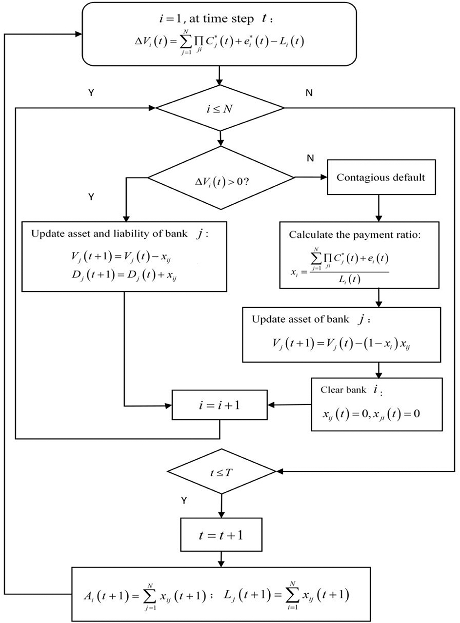
The next step is to clean up all the failed banks in the banking system, then the banking network changes accordingly. We update the lending matrix X^*(t + 1), interbank lending assets A_i(t + 1), and interbank lending liabilities L_i(t + 1) at the next time step in section The Dynamic Evolution of Interbank Market Network. We cycle through the above operations at each time step until the end of the time step T.

The Dynamic Evolution of Interbank Market Network

After calculating the clearing payment vector C^*(t) under the time step t, next we update the interbank borrowing assets A_i(t + 1) and borrowing liabilities L_j(t + 1). Combined with the minimum density method in section Default Algorithms Based on the Dynamic Evolution of Bank Balance Sheet Structure, we update the total interbank borrowing assets and total liabilities constraints to get a new borrowing matrix X^*(t + 1). We can see Figure 2 for the specific evolution flow chart.

FIGURE 2

Figure 2. Flow chart of dynamic evolution of interbank market network.

The Calculation of Banking Systemic Risk under Double risk exposures

This paper defines a basic risk when the total assets of bank i are less than the total liabilities due to the loss of external assets under the impact of credit risk exposure of the real industry. When the total assets of bank j are less than the total liabilities due to the failure of bank i and the inability to recover all the interbank loans (the impact of the interbank market risk exposure), a contagious risk occurs. In the system, under the impact of double risk exposures, a bank's total assets are less than its total liabilities (including basic risk and contagious risk), the bank defaults. In this paper, the basic risk is represented by the basic failure probability FR(t), the contagious risk is represented by the contagious failure probability CR(t), and the systemic risk is represented by the system failure probability SR(t), SR(t) = FR(t) + CR(t).

$\begin{array}{ll}FR(t)=\frac{{\displaystyle \sum _{i=1}^N}TagF{R}_i(t)}{N}& (24)\end{array}$

$\begin{array}{ll}CR(t)=\frac{{\displaystyle \sum _{j=1}^N}TagC{R}_j(t)}{N}& (25)\end{array}$

$\begin{array}{ll}SR(t)=\frac{{\displaystyle \sum _{i=1}^N}TagF{R}_i(t)+{\displaystyle \sum _{j=1}^N}TagC{R}_j(t)}{N}& (26)\end{array}$

Data

This paper uses the balance sheet of Chinese banks in 2016 and the China Securities Regulatory Commission's 2012 version of industry classification Listed Company information in the CSMAR economic and financial database, as well as the data of the 2016 annual report publicly disclosed on the official website. China has a large number of banks, which are mainly divided into six types according to the definition of the CBRC annual report: policy banks, large commercial banks, joint-stock banks, urban commercial banks, rural commercial banks, and foreign banks. By analyzing the collected data, we have found that the same type of banks has the same order of magnitude of assets and liabilities. Moreover, assets and liabilities of policy banks and large commercial banks belong to the same order of magnitude. Consider that the nature and function of banks are irrelevant factors in this study, so policy banks and large commercial banks can be simplified into one type and named large banks. Finally, this paper has divided Chinese banks into five types: large banks, joint-stock banks, urban commercial banks, rural commercial banks, and foreign banks. Due to the limitation of data availability, this paper finally selects 205 banks, which are large banks (8 Banks), joint-stock banks (13 banks), urban commercial banks (102 banks), rural commercial banks (63 banks), and foreign banks (19 banks). It selects individual stock transaction amount in 244 days and balance sheet of 3,017 listed companies in 18 industries that are classified according to the China securities regulatory commission 2012 edition of industry classification guidelines, and then selects loan industry concentration data of 104 banks. For convenience of presentation, the chart in this article indicates 205 banks with numbers 1–205 (see Appendix Table 1 for bank names) and 18 industries with numbers 1–18 (see Appendix Table 2 for industry names). In addition, the descriptive statistics of data can be seen in Appendix Tables 3–6.

Results

The Assessment of Credit Risk of the Real Industry

The Evolution Curve of Credit Risk of the Real Industry

In this paper, the stress test is carried out for the listed companies in 18 real industries to make each Listed Company lose 30% of its assets in the same real industry, so that some listed companies have credit default and the dynamic evolution chart of credit risk in each industry is obtained (see Figure 1B). According to the evolution characteristics of default probabilities in various industries, credit risks in 18 industries can be divided into 4 types that are stability after decline (see Figure 3A), increase in fluctuation (see Figure 3B), decrease in fluctuation (see Figure 3C), fluctuation (see Figure 3D).

FIGURE 3

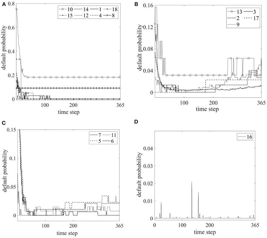
Figure 3. Credit default probability curve of the real industry. (A) Curve of stability after decline. (B) Curve of increasing in fluctuation. (C) Curve of decreasing in fluctuation. (D) Curve of fluctuation.

The evolution of credit risk is characterized by the first decline and then stability in eight industries: finance industry, education industry, water conservancy, environment and public facilities management industry, leasing and business services industry, agriculture, forestry, animal husbandry and fishery industry, electricity, heat, gas and water production and supply industry, comprehensive industry, and accommodation and catering industry. The credit risk of the eight industries decreased within 100 time steps and then stabilized, among which the credit risk of the financial industry stabilized at 0.2, the credit risk of the accommodation and catering industry stabilized at 0.1, and the credit risk of the other six industries stabilized at 0.

The evolution of credit risk is characterized by increase in fluctuation in five industries: scientific research and technology services industry, mining industry, information transmission software and information technology services industry, manufacturing industry, culture, and sports and entertainment industry. Among them, the risk fluctuation range of scientific research and technical services industry is the largest, while the risk fluctuation range of culture, sports and entertainment industry is the smallest. The credit risk of information transmission software and information technology service industry and manufacturing industry showed an evolutionary trend of increasing continuously, while the credit risk of scientific research and technology service industry, mining industry, and culture, sports and entertainment industry showed an evolutionary trend of stabilizing.

The evolution of credit risk is characterized by decrease in fluctuation in four industries: transportation, warehousing and postal industry, construction industry, real estate industry, and wholesale and retail industry. The risk characteristics of these four industries are similar. The failure probability of the industry falls to a certain value within the first 100 time steps, and then fluctuates slightly within the probability range of 0 to 0.05.

The evolution of credit risk in the health and social work industry is characterized by fluctuation, which fluctuates around 0.

Stability of Credit Risk of the Real Industry

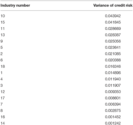
From Figure 3 in The Evolution Curve of Credit Risk of the Real Industry, we can see that the credit risk of 18 real industries has different volatility, indicating that the credit risk of these industries is unstable. Therefore, this section further evaluates the stability of credit risk of the real industry by calculating the variance of credit risk. Table 1 is the result of ranking the variance of credit risk of 18 real industries in descending order. It can be seen that the top three real industries with the largest variance are financial industry, education industry, and real estate industry, that is to say, the credit risk of these three real industries is the most unstable. The real industry with the least variance is health and social work industry, which has the most stable credit risk.

TABLE 1

Table 1. Statistical table of variance of credit risk of each real industry.

Mean Credit Risk of the Real Industry

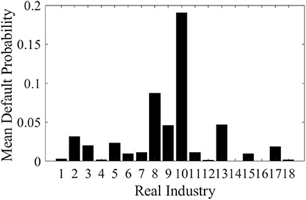
From Figure 3 in section Default Algorithms Based on the Dynamic Evolution of Bank Balance Sheet Structure and Table 1 in section Stability of Credit Risk of the Real Industry, we can see that the dynamic evolution credit risk of real industries presents a fluctuating state, most industries are unstable. It is impossible to accurately assess the value of credit risk of different real industries. Therefore, the next step of this paper is to carry out Monte Carlo simulation in 1000 time steps on the basis of pressure test. In order to eliminate the simulation error as much as possible, this paper adopts the mean value for comparative analysis. We use S_g(t) in Equation (12) and AVG(S_g(t)) is taken as the mean value of the number of enterprise failures in the real industry during 1000 simulations. If the industry credit risk is expressed as P_K in 1,000 simulations, the calculation formula is: $P_K\mathrm{\text{=}}\frac{\sum AVG(S_g(t))}{T\times n_k}$, k = 1, 2, …, 18 indicates 18 industries, T is the dynamic evolution time step 1,000, n_k is number of listed companies in the k industry.

Figure 4 is the result of Monte Carlo simulation of mean credit risk of various industries under 1,000 times. From Figure 4, it can be analyzed that the top four real industries with the highest mean credit risk are: finance, accommodation and catering, scientific research and technical services, and information transmission, and software and information technology services. It is suggested to strengthen the credit risk management of enterprises in the fields of finance, science and technology, and national life. Two real industries with the lowest mean credit risk are: water conservancy environment and public facilities management, and health and social work, while the other 12 real industries have medium mean credit risk.

FIGURE 4

Figure 4. The mean credit risk of the credit industry under the simulation of 1,000 times.

Combined with the industry stability analysis results in section Stability of Credit Risk of the Real Industry, it can be found that the mean credit risk of the financial industry is the highest and the most unstable. The mean credit risk of accommodation and catering industry is high but stable. The mean credit risk and stability of scientific research and technical services, information transmission software and information technology services are relatively high. However, two real industries: water conservancy environment and public facilities management, health and social work, have the lowest mean credit risk and the highest stability.

Default State Analysis of Listed Companies in the Real Industry

The credit risk of the real industry is directly proportional to the number of default listed companies in the industry. In the process of dynamic evolution, the listed companies with higher probability of bankruptcy are more unstable. It can be considered that the enterprises with higher probability of bankruptcy contribute more to the credit risk of the industry.

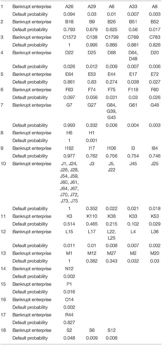
Table 2 shows the top five listed companies in the default probability of 18 industries after stress test. These companies have the largest contribution to the credit risk of their industries, and the default status of listed companies in different industries is significantly different. A total of 17 listed companies in 18 real industries have a default probability of 1 during 1,000 times of dynamic evolution, which belongs to the state of extremely easy default. Among them, 14 listed companies belong to the financial industry. Combined with the mean credit risk results of the real industry in section Mean Credit Risk of the Real Industry, it can be seen that 20% of listed companies in the financial industry are very vulnerable to bankruptcy, and these companies contribute the most to credit risk of financial industry.

TABLE 2

Table 2. Listed companies with the top five bankruptcy frequency in the real industry.

There are no more than three listed companies in five real industries: accommodation and catering industry, water conservancy environment and public facilities management industry, education industry, culture, sports and entertainment industry, and comprehensive industry. In the dynamic evolution process, only two listed companies have the default probability of more than 0.8, and other listed companies have the default probability of <0.1. There are 11 listed companies in the accommodation and catering industry, among which one is very vulnerable to bankruptcy and contributes the most to the credit risk of the accommodation and catering industry.

The top five listed companies in manufacturing, information transmission software and information technology services have a high default probability, which are all over 0.7. However, due to the large number of listed companies in the manufacturing industry, the mean credit risk is not high. The number of listed companies in the information transmission software and information technology services industry is close to one ninth of the manufacturing industry, so the mean credit risk is higher.

The Assessment of Systemic Risk Under Double Risk Exposures

Analysis of the Network Structure With Double Risk Exposures

Credit network structure between banks and the real industry

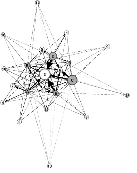
According to the model of credit network between banks and real industry in section Credit Network Between Banks and Real Industry and the data in section Data, the credit network structure diagrams between 5 types of banks and 18 real industries are constructed, as shown in Figure 5. Among them, 18 white circles marked with numbers represent the 18 real industries in which banks provide loans. The circle size reflects the number of listed companies in the real industry. The larger the circle, the more listed companies in the real industry. For example, the number of listed companies in the manufacturing industry is the largest and the circle is the largest. Five gray circles marked with letters indicate five types of banks, which are A (large bank), B (joint-stock bank), C (urban commercial bank), D (rural commercial bank), and E (foreign bank). The circle size indicates the number of banks under this type. The larger the circle, the more banks under this type. The connection between the five types of banks and the real industry means that banks provide loans to the real industry. This paper assumes that each type of banks provides loans to 18 real industries. The line thickness indicates the proportion of loans. Industries with large proportion of loans are concentrated in the center of the map, while industries with small proportion of loans are scattered around.

FIGURE 5

Figure 5. Credit network between banks and real industry.

As can be seen from the thickness of the connection line in Figure 5, the top four real industries with the highest proportion of loans provided by the five types of banks to the real industry are 3 (manufacturing), 6 (wholesale and retail), 11 (real estate), and 12 (leasing and business services), while the lowest industry is 13 (scientific research and technical services). There are differences in the concentration of loans by industries among different types of banks. Table 3 lists the industries with the highest concentration of loans among the five types of banks.

TABLE 3

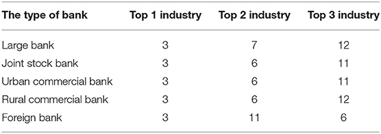
Table 3. Top three real industries with the most loans from banks (the figure in the table is the industry number).

Dynamic evolution of interbank market network structure

We use the minimum density method in section Estimation of the Interbank Market Risk Exposure, interbank market network in section The Dynamic Evolution of Interbank Market Network, and data in section Data to obtain the dynamic evolution of interbank market network structure diagram, as shown in Figures 6A,B, which corresponds to Figure 1D in section Model. Figure 6A shows the network structure diagram of the interbank market at time step t₁. In the Figure 6A, network nodes marked with numbers represent 205 banks, the size of the node indicates the connection degree between banks. The larger the connection degree is, the larger the node is. The directed line between nodes indicates the interbank lending relationship, and the line thickness indicates the lending amount. From Figure 6A, it can be found that there are 8 nodes with relatively large connection degree at time step t₁, which are 190 (industrial and commercial bank of China), 193 (agricultural bank of China), 191 (China construction bank), 194 (bank of China), 82 (bank of communications), 118 (Shanghai Pudong Development Bank), 192 (China Minsheng bank), and 184 (China merchants bank). The connection between these eight nodes is relatively thick, of which the connection from 190 to 193 is the thickest, which indicates that Industrial and Commercial Bank of China lends the largest amount of funds to Agricultural Bank of China. In Figure 6B, the network structure of the interbank market at time step t₁₅₀ has changed compared with time step t₁. The number of network nodes has been reduced to 120 (due to the removal of some default banks from the network), the node size and the connections between nodes have also changed (the interbank lending relationship has changed).

FIGURE 6

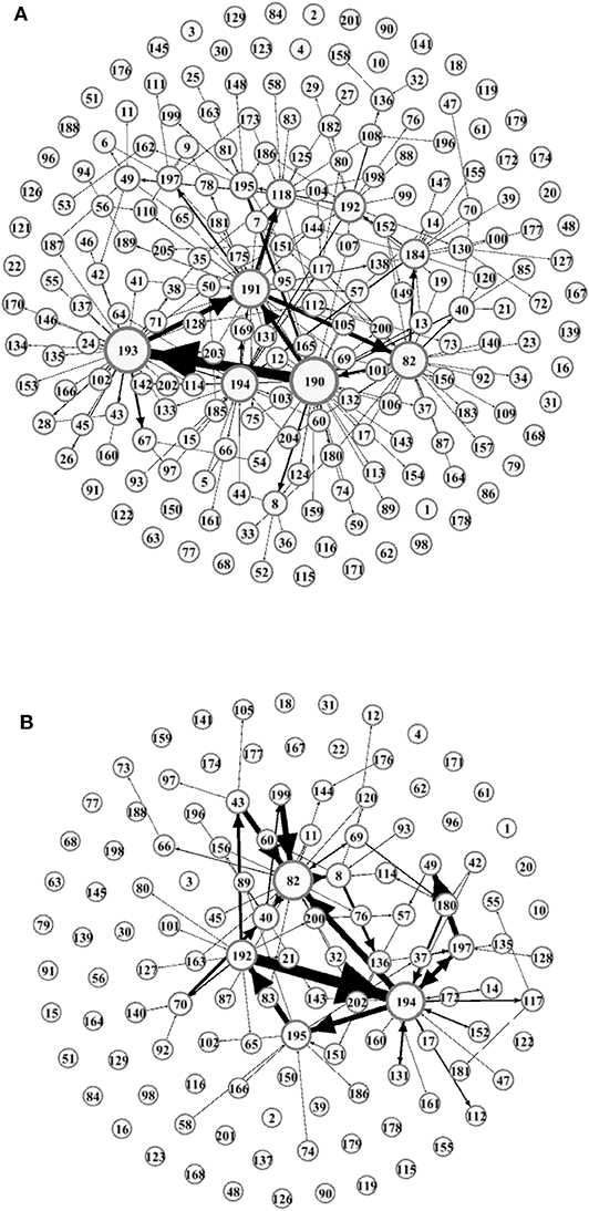
Figure 6. Network structure of interbank market. (A) Represents Chinese interbank market network structure at time step t₁. (B) Represents Chinese interbank market network structure at time step t₁₅₀.

Dynamic Evolution of Systemic Risk in Chinese Banking System

Basic Default, Contagious, and Systemic Risk of Chinese Banks

Figure 7 represents the dynamic evolution law of basic default, contagious, and systemic risk under double risk exposures. It can be seen from the Figure 7 that during the evolution of 365 time steps, the systemic risk has the characteristic of stabilizing after increasing and reaching a stable state at 250 steps. The degree of evolution of contagious risk is higher than that of basic default and the dynamic evolution characteristics of basic default and contagious risk are different. Contagious risk tends to stabilize after increasing and reaching a stable state at 200 steps. The probability of basic default is low and stable in the first 100 time steps, then jumping growth in 101 to 250 time steps, and finally slowing down and stabilizing in 250 steps.

FIGURE 7

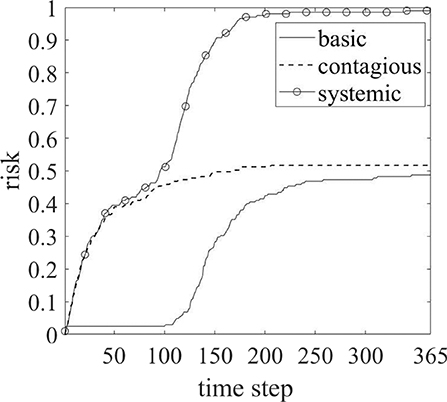
Figure 7. Dynamic evolution curve of basic default, contagious, and systemic risk of Chinese banking system.

Basic Risk, Contagious Risk, and Systemic Risk Characteristics of Different Types of Banks

On the basis of section Basic Default, Contagious, and Systemic Risk of Chinese Banks, this paper further analyzes whether there are differences in basic risk, contagious risk, and systemic risk characteristics of different types of banks under the impact of double risk exposures. Figure 8A represents the basic risk curve of five types of banks, Figure 8B represents the contagious risk curve of five types of banks, and Figure 8C represents the systemic risk curve of five types of banks. On the whole, the dynamic evolution trend of basic risk, contagious risk, and systemic risk in the five types of banks are stable after growth. However, the dynamic characteristics of basic risk, contagious risk, and systemic risk in the five types of banks are different.

FIGURE 8

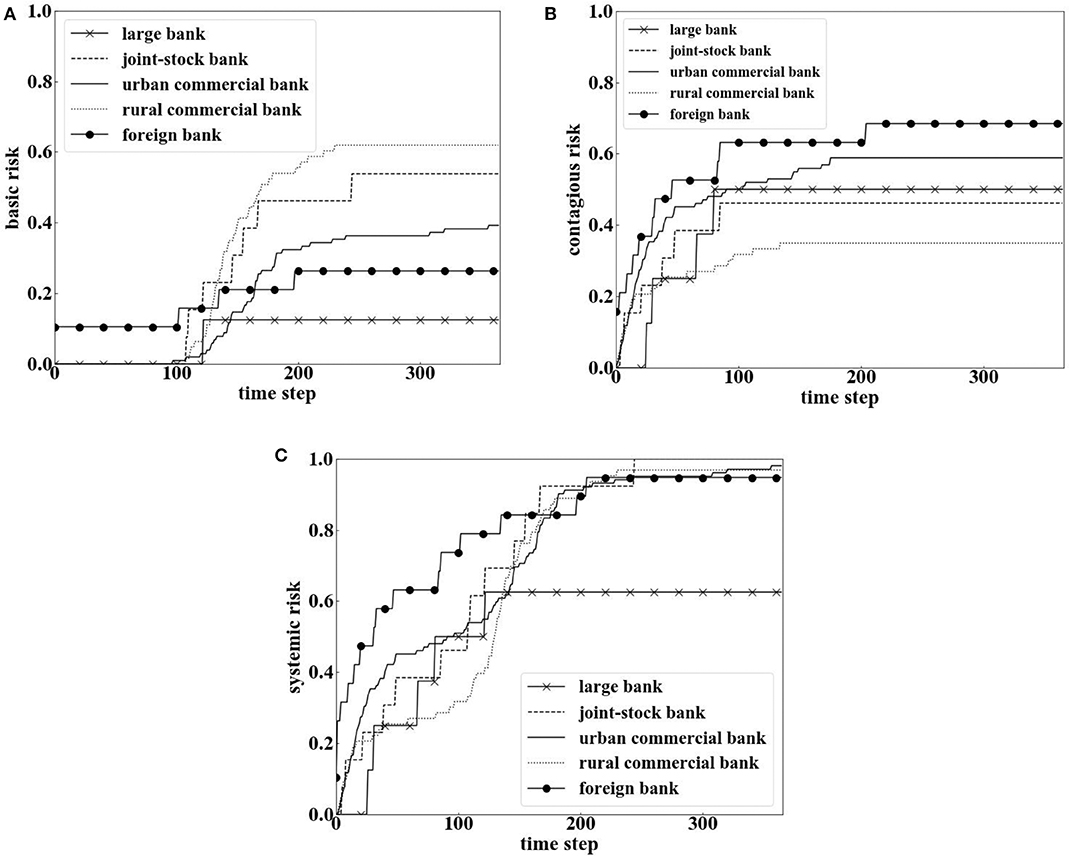
Figure 8. Basic risk, contagious risk, and systemic risk evolution curve of different types of Chinese banks.

In Figure 8A, we can see five types of banks reach a stable state with different time and basic risk finally. The order of basic risk from high to low is: rural commercial bank, joint-stock bank, urban commercial bank, foreign bank, and large bank. The order of time to reach stability from fast to slow is: large bank, foreign bank, rural commercial bank, joint-stock bank, and urban commercial bank.

In Figure 8B, we also can see five types of banks reach a stable state with different time and contagious risk finally. The order of contagious risk from high to low is: foreign bank, urban commercial bank, large bank, joint-stock bank, and rural commercial bank. The order of time to reach stability from fast to slow is: large bank, joint-stock bank, rural commercial bank, urban commercial bank, and foreign bank.

In Figure 8C, the systemic risk of large bank reaches a stable state at the earliest with the lowest risk, while the other four types of banks reach a stable state later with high systemic risk, of which the mean systemic risk of foreign bank is the highest. This reflects that large banks are stronger than the other four types of banks in resisting the impact of double risk exposures, while foreign bank are the weakest.

Discussion and Conclusions

This paper first used Geometric Brownian Motion in physics, Monte Carlo simulation, and real data of the real industry to estimate the dynamic evolution credit risk exposure of the real industry. Then, it used the minimum density method and Chinese real banking data to estimate the more realistic dynamic interbank market risk exposure. So far, we have successfully built up the double risk exposure. Finally, based on the double risk exposure, we use the data of assets, liabilities, and industry loans of 205 Chinese banks, as well as the data of 3017 listed companies' stock market to study the dynamic evolution law of the systemic risk of Chinese banking system. The important conclusions are as follows:

First, our dynamic evolution model highlighted the impact of credit risk exposure and enables to assess which real industries are more/less risky. In addition, we also assessed listed companies with top five bankruptcy frequency of the real industry. Therefore, this information can assist financial regulators to weigh credit loans by credit risk of the real industry/Listed Company. Financial industry, accommodation and catering industry, scientific research and technology service industry, and information transmission software, and technology service industry have higher credit risk, while financial industry, scientific research and technology service industry, and information transmission software and technology service industry have lower stability. It is suggested that financial regulators should pay special attention to the credit risk management of these four real industries when serving the development of the real economy. It is expected that this methodology would engender a reduction in credit loans to risky real industry/Listed Company, leading to a decrease in the systemic risk of Chinese banking system.

Second, the uniqueness of the dataset of Chinese banks and real industries not only permit us to construct credit network and interbank network, but also enables us to broaden other contagion channels apart from classical interbank market. Under the impact of double risk exposures, the systemic risk gradually rises and then reaches a stable state in the evolution process; the contagious risk initially grows faster and then stabilizes; however, the basic default is very small at first, then slowly rises, and finally stabilizes. Further results showed that the dynamic characteristics of the systemic risk in different types of banks are shown as growth first and then stabilization, among which the ability of large banks to resist the impact of double risk exposures is stronger than the other four types of banks, while the ability of foreign bank to resist is the weakest.

The present paper focused on the Chinese system market, however, in the future, the methods proposed can be extended to other global markets or a mature market in other countries. In addition, due to the use of different system risk measurement methods, the results will be different. In the future, we will use other methods to compare with the proposed method, so as to compare the robustness of the proposed method in the present paper.

Data Availability Statement

All datasets generated for this study are included in the article/Supplementary Material.

Author Contributions

HF and WS performed analyses, discussed the results, and wrote the manuscript.

Funding

We are grateful for the support from national natural science foundation of China (71971054) and natural science foundation of Shanghai (19ZR1402100).

Conflict of Interest

The authors declare that the research was conducted in the absence of any commercial or financial relationships that could be construed as a potential conflict of interest.

Supplementary Material

The Supplementary Material for this article can be found online at: https://www.frontiersin.org/articles/10.3389/fphy.2020.00199/full#supplementary-material

References

1. Allen F, Gale D. Financial contagion. J Polit Econ. (2000) 108:1–33. doi: 10.1086/262109

CrossRef Full Text | Google Scholar

2. Freixas X, Parigi B, Rochet JC. Systemic risk, interbank relations and liquidity provision by the central bank. J Money Credit Bank. (2000) 32:611–38. doi: 10.2307/2601198

CrossRef Full Text | Google Scholar

3. Martínez-Jaramillo S, Pérez OP, Embriz FA, Dey FLG. Systemic risk, financial contagion and financial fragility. J Econ Dyn Control. (2010) 34:2358–74. doi: 10.1016/j.jedc.2010.06.004

CrossRef Full Text | Google Scholar

4. Mistrulli PE. Assessing financial contagion in the interbank market: maximum entropy versus observed interbank lending patterns. J Bank Finan. (2011) 35:1114–27. doi: 10.1016/j.jbankfin.2010.09.018

CrossRef Full Text | Google Scholar

5. Ladley D. Contagion and risk-sharing on the interbank market. J Econ Dyn Control. (2013) 37:1384–400. doi: 10.1016/j.jedc.2013.03.009

CrossRef Full Text | Google Scholar

6. Sui C, Chi GT, Wang ZY. Network structure and banking systemic risk. J Manage Sci. (2014) 17:57–70. doi: 10.3969/j.issn.1007-9807.2015.12.002

CrossRef Full Text | Google Scholar

7. Bao Q, Sun YX. Financial structure and financial risk contagion from the perspective of network. Syst Eng Theor Prac. (2014) 34:2202–11. doi: 10.12011/1000-6788(2014)9-2202

CrossRef Full Text | Google Scholar

8. Adrian T, Brunnermeier MK. CoVaR. Technical Report. Department of Economics Princeton University (2011). doi: 10.3386/w17454

CrossRef Full Text | Google Scholar

9. Huang X, Zhou H, Zhu H. Systemic risk contributions. J Finan Serv Res. (2011) 42:55–83. doi: 10.1007/s10693-011-0117-8

CrossRef Full Text | Google Scholar

10. Billio M, Getmansky M, Lo A, Pellizzon L. Econometric measures of connectedness and systemic risk in the finance and insurance sectors. J Finan Econ. (2012) 104:535–59. doi: 10.1016/j.jfineco.2011.12.010

CrossRef Full Text | Google Scholar

11. Ang A, Longstaff FA. Systemic sovereign credit risk: lessons from the U.S. and Europe. J Monet Econ. (2013) 60:493–510. doi: 10.1016/j.jmoneco.2013.04.009

CrossRef Full Text | Google Scholar

12. Diebold F, Yilmaz K. On the network topology of variance decompositions: measuring the connectedness of financial firms. J Econometr. (2014) 182:119–34. doi: 10.1016/j.jeconom.2014.04.012

CrossRef Full Text | Google Scholar

13. Li Z, Liu Q, Liang Q. Research on China's systemic risk prevention based on economic and financial correlation network. Stat Res. (2019) 36:25–39. doi: 10.19343/j.cnki.11-1302/c.2019.02.003

CrossRef Full Text | Google Scholar

14. Zhai YH. A study on risk spillovers between the real industry and the banking sector from the perspective of systemic risk management. Int Finan Res. (2019) 12:74–84. doi: 10.13891/j.cnki.mer.2019.12.009

CrossRef Full Text | Google Scholar

15. Zhu B, Ma YT. Industry characteristics, monetary policy and systemic risk-analysis based on the correlation network of “economy and finance”. Int Finan Res. (2018) 4:22–32. doi: 10.16475/j.cnki.1006-1029.2019.12.008

CrossRef Full Text | Google Scholar

16. Sun L, Zhang Y L, Li JY. The real estate industry spillover effects on the systemic risk of financial institutions research - an empirical analysis of the point of view based on industry and enterprise. Southern Econ. (2020) 2:1–16. doi: 10.16475/j.cnki.1006-1029.2018.04.003

CrossRef Full Text | Google Scholar

17. Lu JG, Wang C. Study on bank risk contagion based on interbank borrowing and joint lending. Mod Econ. (2019) 12:41–8. doi: 10.19592/j.cnki.scje.370208

CrossRef Full Text | Google Scholar

18. Wu YY, Hu RD, Yuan ZZ. Network risk contagion and government rescue in common asset holding. Finan Forum. (2017) 8:37–47. doi: 10.16529/j.cnki.11-4613/f.2017.08.006

CrossRef Full Text | Google Scholar

19. Zhai YH, Bian QM. Bank lending and systemic risk prevention and control—research based on complex network model. Wuhan Finan. (2019) 11:12–22. doi: 10.3969/j.issn.1009-3540.2019.11.002

CrossRef Full Text | Google Scholar

20. Caccioli F, Farmer JD, Foti N, Rockmore D. Overlapping portfolios, contagion, and financial stability. J Econ Dyn Control. (2015) 51:50–63. doi: 10.1016/j.jedc.2014.09.041

CrossRef Full Text | Google Scholar

21. Glasserman P, Young HP. How likely is contagion in financial networks? J Bank Finan. (2015) 50:383–99. doi: 10.1016/j.jbankfin.2014.02.006

CrossRef Full Text | Google Scholar

22. Chiu W-C, Peña JI, Wang C-W. Industry characteristics and financial risk contagion. J Bank Finan. (2015) 50:411–27. doi: 10.1016/j.jbankfin.2014.04.003

CrossRef Full Text | Google Scholar

23. Wang H, Li S. A study on the measurement of systemic risk contagion in China's real estate industry and banking industry from an internal perspective. Int Finan Res. (2015) 9:76–85. doi: 10.16475/j.cnki.1006-1029.2015.09.008

CrossRef Full Text | Google Scholar

24. Li SZ, Ma JL, Zhu SS. The impact of real estate credit on the systemic risk of China's banking system – a simulated empirical study based on the internal lending network of the banking system. J Zhongsan Univ. (2019) 59:186–96. doi: 10.13471/j.cnki.jsysusse.2019.03.020

CrossRef Full Text | Google Scholar

25. Lehar A. Measuring systemic risk: a risk management approach. J Bank Finan. (2005) 29:2577–603. doi: 10.1016/j.jbankfin.2004.09.007

CrossRef Full Text | Google Scholar

26. Black F, Scholes MS. The pricing of options and corporate liabilities. J Polit Econ. (1973) 81:637–54. doi: 10.1086/260062

CrossRef Full Text | Google Scholar

27. Duan J-C. Correction: maximum likelihood estimation using price data of the derivative contract. Math Finan. (2000) 10:461–2. doi: 10.1111/1467-9965.00105

CrossRef Full Text | Google Scholar

28. Anand K, Craig B, Peter GV. Filling in the blanks: network structure and interbank contagion. Quant Finan. (2015) 15:625–36. doi: 10.1080/14697688.2014.968195

CrossRef Full Text | Google Scholar

29. Fan H, Amalia AA, Gao QQ. The assessment of systemic risk in the Kenyan banking sector. Complexity. (2018) 2018:1–15. doi: 10.1155/2018/8767836

CrossRef Full Text | Google Scholar

30. Eisenberg L, Noe TH. Systemic risk in financial systems. Manage Sci. (2001) 47:236–49. doi: 10.1287/mnsc.47.2.236.9835

CrossRef Full Text | Google Scholar