Necessary and Sufficient Conditions for Expressing Quadratic Rational Bézier Curves

Quadratic rational Bézier curve transformation is widely used in the field of computational geometry. In this paper, we offer several important characteristics of the quadratic rational Bézier curve. More precisely, on the basis of proving its monotonicity, the necessary and sufficient conditions for transforming a quadratic rational Bézier curve into a point, line segment, parabola, elliptic arc, circular arc, and hyperbola are proved, respectively.

1. Introduction

Bézier curves have wide application in computer-aided geometric design, being used to provide precisely described points along a given curve [1]. Compared to other methods, such as the French curve, Bézier-based approaches are more computationally affordable and reliable. Additionally, the advantages of the Bézier curve in geometric design include its simple but clear mathematical function [2]. For instance, it is capable of incorporating both conic sections and parametric cubic curves as special cases [3]. As such, one can deal with two different curves simultaneously using one unique computational procedure. Some preliminary studies and applications of Bézier curves can be found in Lu et al. [4], Lee [5], and Han [6].

In this paper, to better understand the basic characteristics of Bézier curves, we conduct some fundamental research. In particular, we discuss the necessary and sufficient conditions for representing six different basic shapes, including a point, line segment, parabola, elliptic arc, circular arc, and hyperbola, using Bézier curves [7, 8]. These results play a fundamental role in the shape formulation and can help in facilitating any subsequent computer-based geometric design.

To begin with, we introduce the mathematical model of the quadratic rational Bézier curve [1].

Definition 1. The quadratic rational Bézier curve is defined as follows:

$\begin{array}{ll}p(t)=\frac{{(1-t)}^2{\omega }_0{P}_0+2t(1-t){\omega }_1{P}_1+t^2{\omega }_2{P}_2}{{(1-t)}^2{\omega }_0+2t(1-t){\omega }_1+t^2{\omega }_2},t\in [0,1],& (1)\end{array}$

where

$\begin{array}{ll}t=\frac{\sqrt{{\omega }_0}\mu }{\sqrt{{\omega }_0}\mu +\sqrt{{\omega }_2}(1-\mu )},\mu \in \left[0,1\right],& (2)\end{array}$

and ω₀ and ω₂ are not zero values at the same time.

The monotonicity of Formula (1.2) is discussed below. Let μ₁ ∈ [0, 1], μ₂ ∈ [0, 1], and μ₁ ≤ μ₂. Accordingly, in the case of μ₁ = 0, we have:

$\begin{array}{ll}{t}_1=\frac{\sqrt{{\omega }_0}{\mu }_1}{\sqrt{{\omega }_0}{\mu }_1+\sqrt{{\omega }_2}(1-{\mu }_1)}=0.& (3)\end{array}$

Note that 1 ≥ μ₂ > μ₁ ≥ 0, and $t_2=\frac{\sqrt{{\omega }_0}{\mu }_2}{\sqrt{{\omega }_0}{\mu }_2+\sqrt{{\omega }_2}(1-{\mu }_2)}\ge 0$; then it is easy to have t₂ ≥ t₁ = 0.

In the case of μ₁ ≠ 0 and μ₂ ≠ 0, according to Formula (1.2), we have:

$\begin{array}{l}\frac{t_1}{t_2}=\frac{\sqrt{{\omega }_0}{\mu }_1}{\sqrt{{\omega }_0}{\mu }_1+\sqrt{{\omega }_2}(1-{\mu }_1)}/\frac{\sqrt{{\omega }_0}{\mu }_2}{\sqrt{{\omega }_0}{\mu }_2+\sqrt{{\omega }_2}(1-{\mu }_2)}\\ =(\sqrt{{\omega }_0}+\sqrt{{\omega }_2}(\frac{1}{{\mu }_2}-1))/(\sqrt{{\omega }_0}+\sqrt{{\omega }_2}(\frac{1}{{\mu }_1}-1))\le 1.& (4)\end{array}$

In other words, we have the conclusion that t is monotonically increasing [9–11]. Furthermore, if we apply linear transformation to Formula (1.1), it is easy to know

$\begin{array}{ll}\begin{array}{l}p(\mu )=\frac{{\omega }_0{\omega }_2{(1-\mu )}^2{P}_0+2\sqrt{{\omega }_0}\sqrt{{\omega }_2}{\omega }_1\mu (1-\mu )P_1+{\omega }_0{\omega }_2{\mu }^2{P}_2}{{\omega }_0{\omega }_2{(1-\mu )}^2+2\sqrt{{\omega }_0}\sqrt{{\omega }_2}{\omega }_1\mu (1-\mu )+{\omega }_0{\omega }_2{\mu }^2}\hfill \\ =({\left(1-\mu \right)}^2{{\rm P}}_0+2\sqrt{\frac{{\omega }_1^2}{{\omega }_0{\omega }_2}}\mu (1-\mu ){{\rm P}}_1+{\mu }^2{{\rm P}}_2)/({\left(1-\mu \right)}^2\hfill \\ +2\sqrt{\frac{{\omega }_1^2}{{\omega }_0{\omega }_2}}\mu (1-\mu )+{\mu }^2).\hfill \end{array}& (5)\end{array}$

Let $\omega =\sqrt{\frac{{\omega }_1^2}{{\omega }_0{\omega }_2}}$ and substitute μ with t in the standard form of the quadratic rational Bézier curve. To this end, we have the simplified version of the quadratic rational Bézier curve, which is expressed as follows:

$\begin{array}{ll}p(t)=\frac{{(1-t)}^2{P}_0+2\omega t(1-t)P_1+t^2{P}_2}{{(1-t)}^2+2\omega t(1-t)+t^2}.& (6)\end{array}$

2. Sufficient and Necessary Conditions for a Quadratic Rational Bézier Curve to Degenerate into a Point

Theorem 1. A quadratic rational Bézier curve degenerates into a point if and only if three control points P₀, P₁, P₂ coincide.

Proof. Assume that the quadratic rational Bézier curve degenerates to a point P_A. That is,

$\begin{array}{r}p(t)=\frac{{(1-t)}^2{P}_0+2\omega t(1-t)P_1+t^2{P}_2}{{(1-t)}^2+2\omega t(1-t)+t^2}=P_A\iff \\ {(1-t)}^2(P_0-P_A)+2t(1-t)\omega (P_1-P_A)+t^2(P_2-P_A)=0.& (7)\end{array}$

As can be seen from Formula (7), when t ∈ (0, 1), we have (1−t)² ≠ 0, t² ≠ 0, 2t(1−t) ≠ 0, so P₀ = P_A, P₁ = P_A, P₂ = P_A. That is, when the quadratic rational Bézier curve degenerates into a point, P₀, P₁, P₂ are the same point of P_A.

On the other hand, when three control points coincide (say, the same point P_A), we know that:

$\begin{array}{ll}p(t)=\frac{{(1-t)}^2{P}_A+2t(1-t)\omega P_A+t^2{P}_A}{{(1-t)}^2+2t(1-t)\omega +t^2}=P_A.& (8)\end{array}$

As can be seen from Formula (8), when three control points P₀, P₁, P₂ coincide, the quadratic rational Bézier curve degenerates into a point [12, 13].

ALGORITHM 1

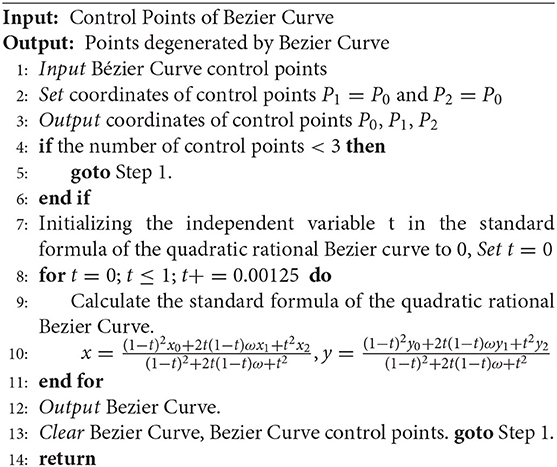
Algorithm 1: To degenerate a Quadratic Rational Bézier Curve into a Point

3. Necessary and Sufficient Conditions for Degradation of a Quadratic Rational Bézier Curve into a Linear Section

Theorem 2. The quadratic rational Bézier curve degenerates into a straight line segment if and only if the control points P₀, P₂ do not coincide, the weight factor ω = 0, or the control point P₁ is on the line segment [14–16].

Proof. First, we assume that one point is with two coordinates; alternatively, we have P₀ = (x₀, y₀), P₁ = (x₁, y₁), and P₂ = (x₂, y₂). As such, for an arbitrary point p(t) = (x, y), according to Formula (6) it is easy to have:

$\begin{array}{l}x=\frac{{(1-t)}^2{x}_0+2t(1-t)\omega x_1+t^2{x}_2}{{(1-t)}^2+2t(1-t)\omega +t^2},\\ y=\frac{{(1-t)}^2{y}_0+2t(1-t)\omega y_1+t^2{y}_2}{{(1-t)}^2+2t(1-t)\omega +t^2},& (9)\end{array}$

On the other hand, a general form for a line function can be expressed as: y = ax + b, where a, and b is a constant [17]. Then, substituting x and y using Formula (12), we can get:

$\begin{array}{l}\frac{{(1-t)}^2{y}_0+2t(1-t)\omega y_1+t^2{y}_2}{{(1-t)}^2+2t(1-t)\omega +t^2}\\ =a\frac{{(1-t)}^2{x}_0+2t(1-t)\omega x_1+t^2{x}_2}{{(1-t)}^2+2t(1-t)\omega +t^2}+b,& (10)\end{array}$

If we simplify the above formula, it is easy to know:

$\begin{array}{ll}(y_0-a{x}_0-b+y_2-a{x}_2-b-2y_1\omega +2a{x}_1\omega +2b\omega )t^2& (11)\end{array}$

$\begin{array}{l}-2(y_0-a{x}_0-b-y_1\omega +a{x}_1\omega +b\omega )t+y_0-a{x}_0-b=0.\end{array}$

First, we assume that one point is with two coordinates; alternatively, we have P₀ = (x₀, y₀), P₁ = (x₁, y₁), and P₂ = (x₂, y₂). As such, for an arbitrary point p(t) = (x, y), according to Formula (6) it is easy to have:

$\begin{array}{l}x=\frac{{(1-t)}^2{x}_0+2t(1-t)\omega x_1+t^2{x}_2}{{(1-t)}^2+2t(1-t)\omega +t^2},\\ y=\frac{{(1-t)}^2{y}_0+2t(1-t)\omega y_1+t^2{y}_2}{{(1-t)}^2+2t(1-t)\omega +t^2},& (12)\end{array}$

Now, control points P₀ and P₂ are the first and last points of the Bézier curve. As they are all on the Bézier curve, they will also be on the straight line [18–20]. Alternatively, we have:

$\begin{array}{ll}{y}_0=a{x}_0+b,y_2=a{x}_2+b.& (13)\end{array}$

Therefore, Formula (11) is further simplified:

$\begin{array}{ll}(y_1-a{x}_1-b)(\omega t-\omega t^2)=0.& (14)\end{array}$

Next, Formula (14) is analyzed in the following aspects:

1. If the control point P₁ is also on the Bézier curve (or on the straight line), then y₁ − ax₁ − b = 0, and Formula (14) clearly holds.

2. If the control point P₁ is not on the Bézier curve (or not on the straight line), then y₁ − ax₁ − b ≠ 0, and Formula (14) can be simplified as

$\begin{array}{ll}-\omega t^2+\omega t=0.& (15)\end{array}$

Therefore, when t ∈ [0, 1], in order to make Formula (15) hold, we have ω = 0.

As such, it is proved that when the quadratic rational Bézier curve degenerates into a straight line segment, two conditions are met: (1) the weight factor ω = 0, or (2) the control point P₁ is on the line segment with the control point P₀, P₂ as the end point. In the following, we discuss these two conditions separately.

1. According to Formula (6), when the weight factor ω = 0, we have:

$\begin{array}{ll}p(t)=\frac{{(1-t)}^2{P}_0+2\omega t(1-t)P_1+t^2{P}_2}{{(1-t)}^2+2\omega t(1-t)+t^2}=\frac{{(1-t)}^2{P}_0+t^2{P}_2}{{(1-t)}^2+t^2},& (16)\end{array}$

and

$\begin{array}{ll}x=\frac{{(1-t)}^2{x}_0+t^2{x}_2}{{(1-t)}^2+t^2}=\frac{{(1-t)}^2{x}_0}{{(1-t)}^2+t^2}+\frac{t^2{x}_2}{{(1-t)}^2+t^2}.& (17)\end{array}$

$\begin{array}{ll}y=\frac{{(1-t)}^2{y}_0+t^2{y}_2}{{(1-t)}^2+t^2}=\frac{{(1-t)}^2{y}_0}{{(1-t)}^2+t^2}+\frac{t^2{y}_2}{{(1-t)}^2+t^2}.& (18)\end{array}$

To simplify the calculation process, let us assume that:

$\begin{array}{ll}\alpha =\frac{{(1-t)}^2}{{(1-t)}^2+t^2}.& (19)\end{array}$

and

$\begin{array}{ll}1-\alpha =\frac{t^2}{{(1-t)}^2+t^2}.& (20)\end{array}$

Now the following formula holds:

$\begin{array}{ll}x=\alpha x_0+(1-\alpha )x_2\to x-x_2=\alpha (x_0-x_2).& (21)\end{array}$

$\begin{array}{ll}y=\alpha y_0+(1-\alpha )y_2\to y-y_2=\alpha (y_0-y_2).& (22)\end{array}$

As the control points P₀, P₂ do not coincide, x₀ ≠ x₂, y₀ ≠ y₂,

$\begin{array}{ll}\alpha =\frac{y-y_2}{y_0-y_2}=\frac{x-x_2}{x_0-x_2}& (23)\end{array}$

$\begin{array}{ll}\frac{y}{y_0-y_2}-\frac{x}{x_0-x_2}=\frac{y_2}{y_0-y_2}-\frac{x_2}{x_0-x_2},& (24)\end{array}$

where x₀, x₂, y₀, y₂ are constants. We assume that $\frac{1}{y_0-y_2}=A,\frac{1}{x_0-x_2}=B,\frac{y_2}{y_0-y_2}-\frac{x_2}{x_0-x_2}=C$ (that is, A,B,C are all constants). Accordingly, we know that Ay − Bx = C is a line segment [21].

2. Let the conditional control point P₁ be the end point (on the line segment with the control points P₀ and P₂) [22]; thus, it can be seen that:

$\begin{array}{ll}{P}_1=(1-v)P_0+v{P}_2,v\in \left[0,1\right],& (25)\end{array}$

The Formula (25) can be substituted with Formula (6) to have:

$\begin{array}{l}p(t)=\frac{{(1-t)}^2+2t(1-t)\omega (1-v)}{{(1-t)}^2+2t(1-t)\omega +t^2}{P}_0\\ +\frac{(2t(1-t)\omega v+t^2}{{(1-t)}^2+2t(1-t)\omega +t^2}{P}_2.& (26)\end{array}$

Then we set:

$\begin{array}{ll}u=\frac{(2t(1-t)\omega v+t^2}{{(1-t)}^2+2t(1-t)\omega +t^2}.& (27)\end{array}$

Comparing Formula (26) with Formula (27), it is easy to find that

$\begin{array}{ll}p(t)=(1-u)P_0+u{P}_2.& (28)\end{array}$

In conclusion, Formula (28) is the parametric formula of the line segment. When the control point P₁ is on the line segment with the control point (P₀, P₂) as the end point, Formula (26) can be written as the parametric formula of the line segment of Formula (28). As such, it is proved that it degenerates into a line segment [23, 24].

ALGORITHM 2

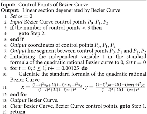
Algorithm 2: To Degenerate a Quadratic Rational Bézier Curve into a Linear section

ALGORITHM 3

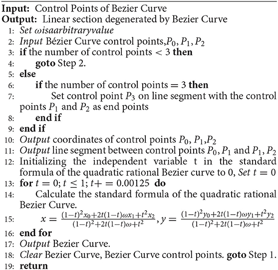
Algorithm 3: To degenerate a Quadratic Rational Bézier Curve into a Linear section

4. Necessary and Sufficient Conditions for a Quadratic Rational Bézier Curve to Represent a Section of Arc

Theorem 3. Quadratic rational Bézier curves can be used to represent an arc if and only if |P₀P₁| = |P₂P₁| and 0 ≤ ω ≤ 1 [25].

Proof. The equation of a circle passing through three collinear points Q_i(x_i, y_i), (i = 1, 2, 3), on a rectangular coordinate plane is:

$\begin{array}{ll}\left|\begin{array}{cccc}{x}^2+y^2& x& y& 1\\ x_0^2+y_0^2& x_0& y_0& 1\\ x_1^2+y_1^2& x_1& y_1& 1\\ x_2^2+y_2^2& x_2& y_2& 1\end{array}\right|=0.& (29)\end{array}$

Given three points that are not collinear, we have:

$\begin{array}{ll}{P}_0(x_0,y_0,0)=(-a,0,0),A(x_A,y_A,0),P_2(x_2,y_2,0)=(a,0,0).& (30)\end{array}$

The arc curve starts from point P₀ and passes through point A to point P₂. Now, let us find another control vertex P₁. To do so, P₀, A, P₂ are substituted into the three-point common-circle equation 29, and we get

$\begin{array}{ll}\left|\begin{array}{cccc}{x}^2+y^2& x& y& 1\\ x_0^2+y_0^2& x_0& y_0& 1\\ x_A^2+y_A^2& x_A& y_A& 1\\ x_2^2+y_2^2& x_2& y_2& 1\end{array}\right|=0.& (31)\end{array}$

From Formula (30) to Formula (31), we can find that x₀ = −a, y₀ = 0, x₂ = a, y₂ = 0. Furthermore, by expanding the determinant 31 in the first row, we have

$\begin{array}{l}(x^2+y^2)\left|\begin{array}{ccc}-a& 0& 1\\ 0& y_A& 1\\ a& 0& 1\end{array}\right|+(-1)x\left|\begin{array}{ccc}{a}^2& 0& 1\\ y_A^2& y_A& 1\\ a^2& 0& 1\end{array}\right|+y\left|\begin{array}{ccc}{a}^2& -a& 1\\ y_A^2& 0& 1\\ a^2& a& 1\end{array}\right|\\ +(-1)\left|\begin{array}{ccc}{a}^2& -a& 0\\ y_A^2& 0& y_A\\ a^2& a& 0\end{array}\right|=0.& (32)\end{array}$

Among them,

$\begin{array}{l}\left|\begin{array}{ccc}-a& 0& 1\\ 0& y_A& 1\\ a& 0& 1\end{array}\right|=-2a{y}_A,\left|\begin{array}{ccc}{a}^2& 0& 1\\ y_A^2& y_A& 1\\ a^2& 0& 1\end{array}\right|=0,\\ \left|\begin{array}{ccc}{a}^2& -a& 1\\ y_A^2& 0& 1\\ a^2& a& 1\end{array}\right|=-a^3+a{y}_A^2+a{y}_A^2-a^3,\\ \left|\begin{array}{ccc}{a}^2& -a& 0\\ y_A^2& 0& y_A\\ a^2& a& 0\end{array}\right|=-a^3{y}_A-a^3{y}_A.& (33)\end{array}$

Finally, the above formula can be simplified as follows:

$\begin{array}{ll}(-2a{y}_A)(x^2+y^2)+y(-a^3+2a{y}_A^2-a^3)+2a^3{y}_A=0.& (34)\end{array}$

Because y_A ≠ 0, it is easy to know

$\begin{array}{ll}{x}^2+{\left(y+\frac{a^2-y_A^2}{2y_A}\right)}^2=a^2+\frac{{(a^2-y_A^2)}^2}{4y_A^2}.& (35)\end{array}$

On the other hand, as x_A = 0, we can add x_A to have

$\begin{array}{ll}{x}^2+{\left(y+\frac{a^2-(x_A^2+y_A^2)}{2y_A}\right)}^2=a^2+\frac{{(a^2-(x_A^2+y_A^2))}^2}{4y_A^2}.& (36)\end{array}$

Summarizing the above formula, the coordinates of the center of the circle O are:

$\begin{array}{ll}{x}_O=0,y_O=\frac{a^2-(x_A^2+y_A^2)}{2y_A}.& (37)\end{array}$

The radius of the circle is:

$\begin{array}{ll}r=\sqrt{a^2+\frac{{(a^2-(x_A^2+y_A^2))}^2}{4y_A^2}}.& (38)\end{array}$

The vertical lines of OP₀ and OP₂ are made from points P₀ and P₂, respectively. According to the symmetry, if two vertical lines intersect with the Y axis at point P₁, then point P₁ is the control vertex of the arc curve. That is,

$\begin{array}{ll}{y}_1=\frac{2a^2{y}_A}{a^2-(x_A^2+y_A^2)}.& (39)\end{array}$

Accordingly, the coordinates of point P₁ are:

$\begin{array}{ll}{x}_1=0,y_1=\frac{2a^2{y}_A}{a^2-(x_A^2+y_A^2)}.& (40)\end{array}$

From the definition of the Bézier Curve in Formula (1), we have:

$\begin{array}{l}x(t)=\frac{{(1-t)}^2{\omega }_0{x}_0+2t(1-t){\omega }_1{x}_1+t^2{\omega }_2{x}_2}{{(1-t)}^2{\omega }_0+2t(1-t){\omega }_1+t^2{\omega }_2},\\ y(t)=\frac{{(1-t)}^2{\omega }_0{y}_0+2t(1-t){\omega }_1{y}_1+t^2{\omega }_2{y}_2}{{(1-t)}^2{\omega }_0+2t(1-t){\omega }_1+t^2{\omega }_2}.& (41)\end{array}$

To simply Formula (41), we further introduce the Quadratic Bernstein Basis Function (B_i,2(t)), which can be expressed as follows:

$\begin{array}{ll}{B}_{0,2}(t)={(1-t)}^2,B_{1,2}(t)=2t(1-t),B_{2,2}(t)=t^2.& (42)\end{array}$

As such, Formula (41) can be rewritten by applying B_i,2(t) in the following format:

$\begin{array}{l}x(t)=\frac{-a{\omega }_0{B}_{0,2}(t)+a{\omega }_2{B}_{2,2}(t)}{{\omega }_0{B}_{0,2}(t)+{\omega }_1{B}_{1,2}(t)+{\omega }_2{B}_{2,2}(t)},\\ y(t)=\frac{2t(1-t){\omega }_1{y}_1}{{\omega }_0{B}_{0,2}(t)+{\omega }_1{B}_{1,2}(t)+{\omega }_2{B}_{2,2}(t)}.& (43)\end{array}$

On the other hand, note that the standard equation of curve arc circle can be estimated as

$\begin{array}{ll}{x}^2(t)+{(y(t)+acot\theta )}^2=a^2/{sin}^2\theta .& (44)\end{array}$

Consequently, by substituting Formulas (43) into Equation (44), the following results are obtained:

$\begin{array}{l}\left(\frac{-a{\omega }_0{B}_{0,2}(t)+a{\omega }_2{B}_{2,2}(t)}{{\omega }_0{B}_{0,2}(t)+{\omega }_1{B}_{1,2}(t)+{\omega }_2{B}_{2,2}(t)}\right){\text{}}^2\\ +\left(\frac{{\omega }_1{y}_1{B}_{1,2}(t)}{{\omega }_0{B}_{0,2}(t)+{\omega }_1{B}_{1,2}(t)+{\omega }_2{B}_{2,2}(t)}+a\cot \theta \right){\text{}}^2=\frac{a^2}{{\sin }^2\theta },& (45)\end{array}$

Note that

$\begin{array}{ll}\frac{a^2}{{sin}^2\theta }-a^2{cot}^2\theta =a^2.& (46)\end{array}$

As such, Formula (45) can be further simplified as

$\begin{array}{r}{a}^2{\omega }_0^2{B}_{0,2}^2(t)+a^2{\omega }_2^2{B}_{2,2}^2(t)-2a^2{\omega }_0{\omega }_2{B}_{0,2}(t)B_{2,2}(t)+{\omega }_1^2{y}_1^2{B}_{1,2}^2(t)\\ +(2{\omega }_1{y}_1{B}_{1,2}(t)a\cot \theta ({\omega }_0{B}_{0,2}(t)+{\omega }_1{B}_{1,2}(t)+{\omega }_2{B}_{2,2}(t))\\ =a^2{({\omega }_0{B}_{0,2}(t)+{\omega }_1{B}_{1,2}(t)+{\omega }_2{B}_{2,2}(t))}^2& (47)\end{array}$

Furthermore, according to Formula (38) and Formula (40), we can have

$\begin{array}{ll}{y}_{1}cot\theta =\frac{2a^2{y}_A}{a^2-(x_A^2+y_A^2)}\times \frac{(a^2-(x_A^2+y_A^2))}{2a{y}_A}=a,& (48)\end{array}$

and then,

$\begin{array}{ll}(y_1^2+a^2){\omega }_1^2{B}_{1,2}^2(t)-4a^2{\omega }_0{\omega }_2{B}_{0,2}(t)B_{2,2}(t)=0.& (49)\end{array}$

Again, we consider the Quadratic Bernstein Basis Function, and then the above formula (in Formula 49) can be simplified as follows:

$\begin{array}{ll}((y_1^2+a^2){\omega }_1^2-a^2{\omega }_0{\omega }_2){(1-t)}^2{t}^2=0.& (50)\end{array}$

Next, according to Formula (40), we know

$\begin{array}{ll}({\omega }_1^2{sec}^2\theta -{\omega }_0{\omega }_2){(1-t)}^2{t}^2=0,& (51)\end{array}$

and t ∈ (0, 1), t²(1 − t)² ≠ 0. It is thus easy to know

$\begin{array}{ll}{\omega }_1^2={\omega }_0{\omega }_2{cos}^2\theta .& (52)\end{array}$

According to the standard form of the quadratic rational Bézier curve (see Formula 6), we can further estimate ω₀ = ω₂ = 1, ω₁ = cosθ, and the value range of θ of the center angle of the semicircle should be 0 ≤ θ ≤ π/2 [26].

In summary, the rational quadratic Bézier expressions of arc curves passing through points P₀, A, P₂ are as follows,

$\begin{array}{ll}C(t)=\frac{{(1-t)}^2{P}_0+2cos(\theta )t(1-t)P_1+t^2{P}_2}{{(1-t)}^2+2cos(\theta )t(1-t)+t^2}.& (53)\end{array}$

Compared with the standard formula of a rational quadratic Bézier, the following results are obtained,

$\begin{array}{ll}\omega =cos(\theta ),& (54)\end{array}$

where 0 ≤ θ ≤ π/2, 0 ≤ ω ≤ 1. Consequently, the necessary and sufficient conditions for a rational quadratic Bézier curve to represent a circular arc are expressed as follows:

$\begin{array}{ll}\left|P_0{P}_1\right|=\left|P_2{P}_1\right|and0\le \omega \le 1.& (55)\end{array}$

ALGORITHM 4

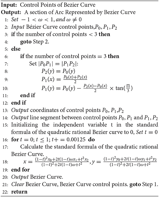
Algorithm 4: For a Quadratic Rational Bézier Curve to Represent a section of an Arc

5. Necessary and Sufficient Conditions for Quadratic Rational Bézier Curves to Represent a Parabola, Elliptic Arc and Hyperbola

Theorem 4. Quadratic rational Bézier curve represents a parabola, elliptic arc, and hyperbola if and only if ω = ±1, −1 < ω < 1, and ω < −1 or ω> 1, respectively [27].

Proof. According to the second order Bernstein basis function of Formula (42), Bézier curve from Formula (1) is written as follows,

$\begin{array}{ll}p(t)=\frac{{\omega }_0{B}_{0,2}(t)P_0}{{\displaystyle \sum _{j=0}^2}{B}_{j,2}(t){\omega }_j}+\frac{{\omega }_1{B}_{1,2}(t)P_1}{{\displaystyle \sum _{j=0}^2}{B}_{j,2}(t){\omega }_j}+\frac{{\omega }_2{B}_{2,2}(t)P_2}{{\displaystyle \sum _{j=0}^2}{B}_{j,2}(t){\omega }_j}={\displaystyle \sum _{i=0}^2}{R}_{i,2}(t)P_i,& (56)\end{array}$

where

$\begin{array}{ll}{R}_{i,2}(t)=\frac{{\omega }_i{B}_{i,2}(t)}{{\displaystyle \sum _{j=0}^2}{B}_{j,2}(t){\omega }_j}.& (57)\end{array}$

Next, we introduce the Local Oblique Coordinate System P₁, S, T, so that S = P₀ − P₁, T = P₂ − P₁. Since point P(t) is within δP₀P₁P₂ for arbitrary t ∈ [0, 1], P(t) can be rewritten as

$\begin{array}{l}P(t)=P_1+u(t)S+v(t)T\\ =P_1+u(t)(P_0-P_1)+v(t)(P_2-P_1)\\ =u(t)P_0+\left[1-u(t)-v(t)\right]P_1+v(t)P_2.& (58)\end{array}$

Comparing the coefficients from both Formula (56) and Formula (58), we know that

$\begin{array}{ll}\begin{array}{c}{R}_{0,2}(t)=u(t),\hfill \\ R_{1,2}(t)=1-u(t)-v(t),\\ R_{2,2}(t)=v(t).\hfill \\ \end{array}\hfill & (59)\end{array}$

Let $k={\omega }_0{\omega }_2/{\omega }_1^2$, where k is the shape-invariant factor of a conic, so

$\begin{array}{ll}u(t)v(t)=R_{0,2}(t){Ṙ}_{2,2}(t)=\frac{1}{4}k{\left[1-u(t)-v(t)\right]}^2.& (60)\end{array}$

Formula (60) is an implicit equation of a quadratic curve in the local oblique coordinate system P₁, S, T. The expansion of Formula (60) further indicates that:

$\begin{array}{ll}k{u}^2(t)+(2k-4)u(t)v(t)+k{v}^2(t)-2ku(t)-2kv(t)+k=0.& (61)\end{array}$

In the Cartesian coordinate system, the image of a binary quadratic equation can represent a conic curve, and all conic curves can be derived in the aforementioned way [1]. The equation has the following forms [28]:

$\begin{array}{ll}A{x}^2+Bxy+C{y}^2+Dx+Ey+F=0,A,B,Carenotallzero,& (62)\end{array}$

where A, B, C, D, E, F are polynomial coefficients. If the following conditions are satisfied,

$\begin{array}{ll}{B}^2-4AC<0,& (63)\end{array}$

then Formula (62) represents an ellipse; furthermore, under the same condition, if the conic degenerates (that is, A = C, B = 0), the equation represents a circle. Additionally, if the following conditions are satisfied,

$\begin{array}{ll}{B}^2-4AC=0,& (64)\end{array}$

then Formula (62) represents a parabola [29]. Finally, if the following conditions are satisfied,

$\begin{array}{ll}{B}^2-4AC>0& (65)\end{array}$

then Formula (62) represents an hyperbola. The coefficients from Formula (61) and Formula (62) can be obtained as follows: A = k, B = k − 2, C = k, D = −2k, E = −2k, F = k. As such, we can get:

$\begin{array}{ll}{B}^2-4AC=1-k.& (66)\end{array}$

ALGORITHM 5

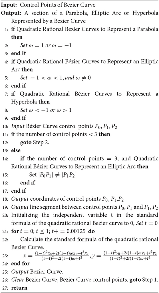
Algorithm 5: For Quadratic Rational Bézier Curves to Represent a Parabola, Elliptic Arc and Hyperbola

We then provide the discussion and judgment of Formula (66). That is, from the condition of Formula (63), if the curve is an ellipse, then in Formula (66) we have B² − 4AC = 1 − k < 0. Therefore, when k > 1, the curve is an ellipse. From the condition of (64), if the curve is a parabola, then B² − 4AC = 1 − k = 0 (again see Formula 66). Therefore, when k = 1, the curve is a parabola. From the condition of 65, if the curve is a hyperbola, then B² − 4AC = 1 − k > 0, so when k < 1, the curve is a hyperbola.

Note that $k={\omega }_0{\omega }_2/{\omega }_1^2$. In summary, under the standard form of the quadratic rational Bézier curve, we have ω₀ = ω₂ = 1, and ω = ω₁. Consequently, we prove that when −1 < ω < 1, the quadratic rational Bézier curve is a ellipse; when ω = ±1, the quadratic rational Bézier curve is a parabola; when ω < −1, or ω > 1, the quadratic rational Bézier curve is a hyperbola.

6. Conclusion

In this paper, we discuss the necessary and sufficient conditions for utilizing quadratic rational Bézier curves to represent different shapes, such as a point, line segment, parabola, elliptic arc, circular arc, and hyperbola. These results can be further used to facilitate other computer-aided geometric designs.

Data Availability Statement

The raw data supporting the conclusions of this article will be made available by the authors, without undue reservation.

Author Contributions

CY: conceptualization, methodology, software, validation, investigation, visualization, and writing original draft. JY: software, writing - review & editing, and supervision. YL: software, visualization, and writing - original draft. XG: writing - review & editing, validation, and visualization.

Funding

This work was supported by the National Natural Science Foundation of China (Grant No. 61873004, 51874003) and the Humanities and Social Sciences Foundation of Anhui Department of Education, China (Grant No. SK2017A0098). We would also like to thank JY from the University of Wollongong for his useful discussion.

Conflict of Interest

The authors declare that the research was conducted in the absence of any commercial or financial relationships that could be construed as a potential conflict of interest.

References

1. Walton DJ, Meek DS. G2 curve design with planar quadratic rational Bézier spiral segments. Int J Comput Math. (2013) 90:325–40. doi: 10.1080/00207160.2012.716831

CrossRef Full Text | Google Scholar

2. Zhang R. Improved derivative bounds of the rational quadratic Bézier curves. Appl Math Comput. (2015) 250:492–6. doi: 10.1016/j.amc.2014.10.120

CrossRef Full Text | Google Scholar

3. Shi M. Degree reduction of disk rational Bézier curves using multi-objective optimization techniques. Int J Appl Math. (2015) 45:392–7.

Google Scholar

4. Lu L, Jiang C, Xiang X. Some remarks on weighted Lupaş [formula omitted]-Bézier curves. J Comput Appl Math. (2017) 313:393–6.

Google Scholar

5. Lee E. The rational Bézier representation for conics. Geometr Model. (1987) 3:5–19.

Google Scholar

6. Han X. Quadratic trigonometric polynomial curves concerning local control. Appl Numer Math. (2006) 56:105–15. doi: 10.1016/j.apnum.2005.02.013

CrossRef Full Text | Google Scholar

7. Samreen S, Sarfraz M, Hussain MZ, Livesu M. Computer aided design using a rational quadratic trigonometric spline with interval shape control. In: 2017 International Conference on Computational Science and Computational Intelligence. Las Vegas, NV: IEEE (2017). p. 246–51.

Google Scholar

8. Bashir U, Abbas MA, Ali JA. The G2 and C2 rational quadratic trigonometric Bézier curve with two shape parameters with applications. Appl Math Comput. (2013) 219:10183–97. doi: 10.1016/j.amc.2013.03.110

CrossRef Full Text | Google Scholar

9. Xu C, Kim T, Farin GE. The eccentricity of conic sections formulated as rational Bézier quadratics. Comput Aided Geometr Des. (2010) 27:458–60. doi: 10.1016/j.cagd.2010.04.001

CrossRef Full Text | Google Scholar

10. Bastl B, Jttler B, Lvicka M, Schicho J, Sír Z. Spherical quadratic Bézier triangles with chord length parameterization and tripolar coordinates in space. Comput Aided Geometr Des. (2011) 28:127–34. doi: 10.1016/j.cagd.2010.11.001

CrossRef Full Text | Google Scholar

11. Hussain MZ, Irshad M, Sarfraz M, Zafar N. Interpolation of discrete time signals using cubic functions. In: IEEE International Conference on Information Visualization. Chicago, IL: IEEE (2015). p. 454–9.

Google Scholar

12. Han L, Wu Y, Chu Y. Weighted Lupaş q-Bézier curves. J Comput Appl Math. (2016) 308:318–29. doi: 10.1016/j.cam.2016.06.017

CrossRef Full Text | Google Scholar

13. Han L-W, Chu Y, Qiu Z-Y. Generalized Bézier curves and surfaces based on Lupaş q-analogue of Bernstein operator. J Comput Appl Math. (2014) 261:352–63. doi: 10.1016/j.cam.2013.11.016

CrossRef Full Text | Google Scholar

14. Cattiaux-Huillard I, Albrecht G, Hernández-Mederos V. Optimal parameterization of rational quadratic curves. Comput Aided Geometr Des. (2009) 26:725–32. doi: 10.1016/j.cagd.2009.03.008

CrossRef Full Text | Google Scholar

15. Hussain M, Saleem S. C¹ rational quadratic trigonometric spline. Egypt Inform J. (2013) 14:211–20. doi: 10.1016/j.eij.2013.09.002

CrossRef Full Text | Google Scholar

16. Sarfraz M, Samreen S, Hussain MZ. Modeling of 2D objects with weighted Quadratic Trigonometric Spline. In: 13th International Conference on Computer Graphics, Imaging and Visualization. Beni Mellal (2016). p. 29–34.

Google Scholar

17. Lee T-K, Baek S-H, Choi Y-H, Oh S-Y. Smooth coverage path planning and control of mobile robots based on high resolution grid map representation. Robot Auton Syst. (2011) 59:801–12. doi: 10.1016/j.robot.2011.06.002

CrossRef Full Text | Google Scholar

18. Han X. Shape preserving piecewise rational interpolant with quartic numerator and quadratic denominator. Appl Math Comput. (2015) 251:258–74. doi: 10.1016/j.amc.2014.11.067

CrossRef Full Text | Google Scholar

19. Lamnii A, Oumellal F. A method for local interpolation with tension trigonometric spline curves and surfaces. Appl Math Sci. (2015) 9:3019–35. doi: 10.12988/ams.2015.52154

CrossRef Full Text | Google Scholar

20. Shi M. Degree reduction of classic disk rational Bézier curves in L₂ Norm. In: 2015 14th International Conference on Computer-Aided Design and Computer Graphics. Xi'an: IEEE (2015). p. 202–3.

Google Scholar

21. Xu A, Viriyasuthee C, Rekleitis I. Efficient complete coverage of a known arbitrary environment with applications to aerial operations. Auton Robot. (2014) 36:365–81. doi: 10.1007/s10514-013-9364-x

CrossRef Full Text | Google Scholar

22. Khan A, Noreen I, Habib Z. Coverage path planning of mobile robots using rational quadratic Bézier spline. In: 2016 International Conference on Frontiers of Information Technology. Islamabad: IEEE (2016). p. 319–23.

Google Scholar

23. Backman J, Piirainen P, Oksanen T. Smooth turning path generation for agricultural vehicles in headlands. Biosyst Eng. (2015) 139:76–86. doi: 10.1016/j.biosystemseng.2015.08.005

CrossRef Full Text | Google Scholar

24. Yu X, Roppel TA, Hung JY. An optimization approach for planning robotic field coverage. In: 41st Annual Conference of the IEEE Inductrial Electronics Society. Yokohama: IEEE (2015). p. 76–86.

Google Scholar

25. Sara E, Pieter P. Exploiting lattice structures in shape grammar implementations. AI EDAM. (2018) 32:147–61. doi: 10.1017/S0890060417000282

CrossRef Full Text | Google Scholar

26. Li Y, Deng C, Jin W, Zhao N. On the bounds of the derivative of rational Bézier curves. Appl Math Comput. (2013) 219:10425–33. doi: 10.1016/j.amc.2013.04.042

CrossRef Full Text | Google Scholar

27. Deng C, Li Y, Mu X, Zhao Y. Characteristic conic of rational bilinear map. J Comput Appl Math. (2019) 346:277–83. doi: 10.1016/j.cam.2018.07.012

CrossRef Full Text | Google Scholar

28. LiZheng L, ChengKai J. Some remarks on weighted Lupaş[formula omitted]-Bézier curves. J Comput. Appl. Math. (2017) 313:393–6. doi: 10.1016/j.cam.2016.09.044

CrossRef Full Text | Google Scholar

29. Yan K, Cheng H-L, Ji Z, Zhang X, Lu H. Accelerating smooth molecular surface calculation. J Math Biol. (2018) 76:779–93. doi: 10.1007/s00285-017-1156-z

PubMed Abstract | CrossRef Full Text | Google Scholar