 Ivan Y. Vasko
 Rachel Wang
 Forrest S. Mozer
 Stuart D. Bale1,2
 Anton V. Artemyev
- 1Space Sciences Laboratory, University of California, Berkeley, Berkeley, CA, United States
- 2Department of Physics, University of California, Berkeley, Berkeley, CA, United States
- 3Institute of Geophysics and Planetary Physics, University of California, Los Angeles, Los Angeles, CA, United States
- 4Space Research Institute of Russian Academy of Sciences, Moscow, Russia
We present a statistical analysis of large-amplitude bipolar electrostatic structures measured by Magnetospheric Multiscale spacecraft in the Earth's bow shock. The analysis is based on 371 large-amplitude bipolar structures collected in nine supercritical quasi-perpendicular Earth's bow shock crossings. We find that 361 of the bipolar structures have negative electrostatic potentials, and only 10 structures (< 3%) have positive potentials. The bipolar structures with negative potentials are interpreted in terms of ion phase space holes produced by ion streaming instabilities, particularly the two-stream instability between incoming and reflected ions. We obtain an upper estimate for the amplitudes of the ion phase space holes that is in agreement with the measurements. The bipolar structures with positive potentials could be electron phase space holes produced by electron two-stream instabilities. We argue that the negligible number of electron phase space holes among large-amplitude bipolar structures is due to the electron hole transverse instability, the criterion for which is highly restrictive at ωpe/ωce ≫ 1, a parameter range typical of collisionless shocks in the heliosphere and various astrophysical environments. Our analysis indicates that the original mechanism of electron surfing acceleration involving electron phase space holes is not likely to be efficient in realistic collisionless shocks.
1. Introduction
The Earth's bow shock is a natural laboratory for probing plasma processes in supercritical collisionless shocks, because the Alfvén Mach number of the solar wind flow typically exceeds the second critical value [1]. Of vital importance in the physics of collisionless shocks are the origin and consequences of various wave activities produced in the shock transition region under realistic background plasma parameters [2, 3]. In particular, there is currently a lack of a thorough understanding of the origin and consequences of electrostatic fluctuations measured in the Earth's bow shock [4–6], which are likely present in astrophysical shocks as well [7–9]. Numerical simulations have demonstrated that electrostatic fluctuations and coherent electrostatic structures produced by various instabilities in a shock transition region can result in efficient electron acceleration (surfing and stochastic surfing mechanisms) at high Mach numbers typical of various astrophysical shocks [8–12] and at low Mach numbers typical of the Earth's bow shock [13]. However, the efficiency of those acceleration processes in realistic collisionless shocks, where typical background plasma parameters are hardly achievable in modern numerical simulations, remains poorly understood. Among the critical background plasma parameters is ωpe/ωce, the ratio of the electron plasma frequency to the electron cyclotron frequency [8], which is typically large in space and astrophysical plasmas [14] but much smaller in numerical simulations of collisionless shocks [3, 15]. The analysis of spacecraft measurements in the Earth's bow shock characterized by ωpe/ωce ~ 100 should advance our understanding of the origin and consequences of electrostatic fluctuations in collisionless shocks under realistic background plasma parameters.
Spacecraft measurements in the Earth's bow shock showed that electric field fluctuations above a few hundred hertz tend to be electrostatic [5, 16, 17]. Analyses of waveform measurements demonstrated that the electrostatic wave activity is produced by ion-acoustic waves [4, 18–21], bipolar electrostatic structures [22–27], electron cyclotron harmonics [6, 28], and low-hybrid waves [29]. The ion-acoustic waves have electric field oriented generally oblique to the magnetic field, wavelengths on the order of a few tens of Debye lengths, and amplitudes of up to a few hundred mV/m [4, 20, 21, 30]. The bipolar structures have similar properties, except that their spatial scales are of only a few Debye lengths [23, 25–27].
The bipolar structures originally measured aboard the Wind spacecraft were interpreted in terms of electron phase space holes [23, 24], which are coherent structures with positive electrostatic potentials appearing in a nonlinear stage of various electron streaming instabilities [31–33]. However, detailed analyses of bipolar structures measured in several crossings of the Earth's bow shock by Cluster spacecraft [25] and Magnetospheric Multiscale spacecraft (MMS) [26, 27] showed that the bipolar structures had negative electrostatic potentials, which is inconsistent with the interpretation in terms of electron phase space holes. Wang et al. [27] have recently considered more than one hundred bipolar structures measured in a particular crossing of the Earth's bow shock and provided strong arguments that the bipolar structures are ion phase space holes produced by the two-stream instability between incoming and reflected ions. The ion two-stream instability was hypothesized to be a source of electrostatic fluctuations in the Earth's bow shock early on by Formisano and Torbert [18], Akimoto and Winske [34], and Fuselier et al. [35], but there have been no strong arguments in favor of that hypothesis until the recent MMS measurements [27].
The analysis of bipolar structures based on MMS measurements is currently restricted to a few of the Earth's bow shock crossings [26, 27]. In this paper we present results of a statistical analysis of bipolar structures measured by MMS in nine crossings of the Earth's bow shock. The analysis provides valuable information on instabilities operating in the Earth's bow shock and reveals the presence, albeit in negligible numbers, of bipolar structures with positive potentials, which could be electron phase space holes. The rarity of electron phase space holes among large-amplitude bipolar structures is most likely due to the electron hole transverse instability, the criterion for which is strongly dependent on ωpe/ωce [36, 37]. We discuss the implications of our results for the surfing acceleration mechanism, which suggested that electron phase space holes might be involved in efficient electron acceleration in high-Mach-number collisionless shocks [10, 11].
2. MMS Observations
To collect a statistically representative dataset of bipolar electrostatic structures, we considered nine crossings of the Earth's bow shock by MMS. The selection criteria for the bow shock crossings were the presence of continuous measurements in burst mode in the shock transition region, a quasi-perpendicular configuration, and a supercritical regime of the shock, that is, an Alfvén Mach number MA greater than 3. The selected Earth's bow shock crossings are listed in Table 1. We note that shocks #6 and #8 were previously considered by Vasko et al. [26] and Wang et al. [27], but the analysis of Vasko et al. [26] was restricted to a few bipolar structures, while Wang et al. [27] excluded from consideration a far-downstream region of the shock. We used measurements taken by the following instruments aboard the MMS: DC-coupled magnetic field at 128 S/s (samples per second) provided by Digital and Analogue Fluxgate Magnetometers [38], AC-coupled electric fields at 8,192 S/s provided by Axial Double Probe [39], and Spin-Plane Double Probe [40], and electron moments at 0.03 s cadence and ion moments at 0.15 s cadence provided by the Fast Plasma Investigation instrument [41]. The electric field was measured by four voltage-sensitive spherical probes on 60 m antennas in the spacecraft spin plane (almost in the ecliptic plane) and two probes on roughly 15 m axial antennas along the spin axis (almost perpendicular to the ecliptic plane). The voltages of the opposing probes measured with respect to the spacecraft are used to compute the electric field and estimate the velocity of propagation and other parameters of bipolar electrostatic structures [26, 42]. Because the spatial scales of bipolar structures are generally comparable to the antenna lengths, corresponding correction factors are included to accurately estimate the electric fields (see Vasko et al. [26] for methodological details).
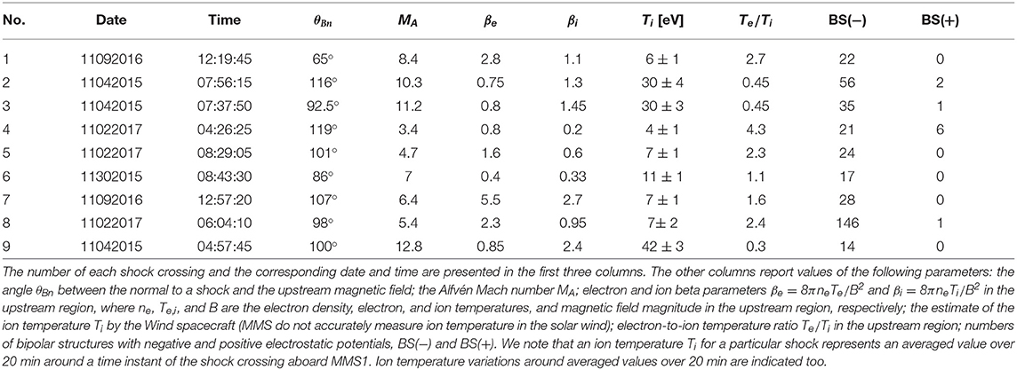
Table 1. Summary of parameters of the Earth's bow shock crossings presented in Figure 1.
Figure 1 presents an overview of the selected Earth's bow shock crossings. The panels display the magnetic field magnitude and parallel electron temperature measured aboard MMS1. The perpendicular electron temperature is almost identical to the parallel temperature (not shown here), because in supercritical shocks the macroscopic electron heating is essentially isotropic [43, 44]. The other MMS located within a few tens of kilometers of MMS1 yield essentially identical overviews of the shocks. The dates and time intervals corresponding to the shocks are shown in the panels, while Table 1 presents estimates of the Alfvén Mach number MA and angle θBn between the upstream magnetic field and the shock normal. The selected shocks are supercritical and quasi-perpendicular, with 3 ≲ MA ≲ 13 and . The shock normals were assumed to be directed toward the upstream region and estimated using the procedure of Vinas and Scudder [45], which is based on considering the Rankine-Hugoniot conditions. Table 1 also presents estimates of the ion and electron beta parameters βi and βe, the ion temperature Ti, and the electron-to-ion temperature ratio Te/Ti in the upstream region. Because MMS measurements of the ion temperature in the solar wind are not accurate, we used ion temperature measurements by the Wind spacecraft1 located at the L1 Earth-Sun Lagrange point, which is about two hundred of Earth's radius upstream of the Earth's bow shock. An ion temperature estimate Ti shown in Table 1 for a particular shock represents an averaged value over 20 min around a time instant of the shock crossing aboard MMS1. Ion temperature variations around an averaged value over these 20 min are also shown in Table 1 and demonstrate that the presented estimates of Ti and hence βi are rather reliable.
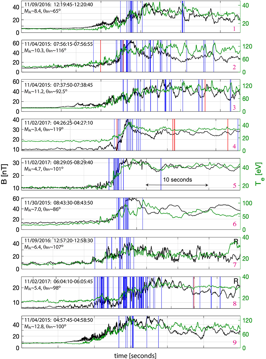
Figure 1. Overview of nine crossings of the Earth's bow shock obtained by Magnetospheric Multiscale spacecraft (MMS). Each panel shows the magnetic field magnitude (black) and parallel electron temperature (green) measured aboard MMS1. The other MMS located within a few tens of kilometers of MMS1 yield essentially identical overviews. The date, time interval, Alfvén Mach number MA, and angle θBn between the upstream magnetic field and the shock normal are indicated in the panels. The other parameters of the shocks are presented in Table 1. In each panel the time interval between two ticks is 10 s. The vertical lines indicate the occurrence of bipolar structures with electric field amplitudes exceeding 50 mV/m. The blue and red lines correspond to bipolar structures with negative and positive electrostatic potentials, respectively. In shocks #7 and #8 the MMS crossed the Earth's bow shock from downstream to upstream, so the crossing is reversed in these panels and therefore marked by R.
Figure 2 presents the electric field measured by MMS1 at 8,192 S/s in shock #8. The electric field magnitude shown in Figure 2A demonstrates that the electric field fluctuations reach amplitudes of up to a few hundred mV/m. Figure 2B displays the electric field in a local magnetic field-aligned coordinate system measured over the 35 ms interval highlighted in Figure 2A. We can see that some of the intense electric field fluctuations correspond to bipolar electrostatic structures. The bipolar structures are noticeable in the electric field components both parallel and perpendicular to the local magnetic field, thereby indicating that the electric fields of the bipolar structures are oriented oblique to the magnetic field, typically at a few tens of degrees [26]. We looked through the electric fields measured aboard the four MMS in the selected Earth's bow shock crossings and collected a dataset of 371 bipolar structures with electric field amplitudes exceeding 50 mV/m. The selection was restricted to large-amplitude bipolar structures to make a careful analysis of these structures feasible. The selection procedure, based on visual inspection, is subjective and probably not exhaustive, but it is adequate enough for collecting a representative dataset of bipolar structures. In the resulting dataset the ratio between the maximum and minimum values of any bipolar electric field does not exceed 2, and for more than 95% of the structures the ratio was below 1.5, so that the selected structures may indeed be referred to as bipolar structures. In addition to bipolar structures, large-amplitude electric field fluctuations in the Earth's bow shock are produced by electrostatic wave-packets and tripolar structures (Figure 2B). The electrostatic wave-packets and the bipolar and tripolar structures are highly likely to be from a common origin (produced by the same instability or instabilities), but in this study we concentrate purely on bipolar structures. The occurrence of the selected bipolar structures in shock transition regions is demonstrated in Figure 1, while Table 1 gives the number of bipolar structures selected in each shock. The number of bipolar structures can be rather different in various shocks, but none of the parameters MA, θBn, βe, βi, and Te/Ti in Table 1 can explain the observed variation in the number of bipolar structures from one shock to another. In what follows, we explain the methodology and present results of the statistical analysis of the selected large-amplitude bipolar structures.
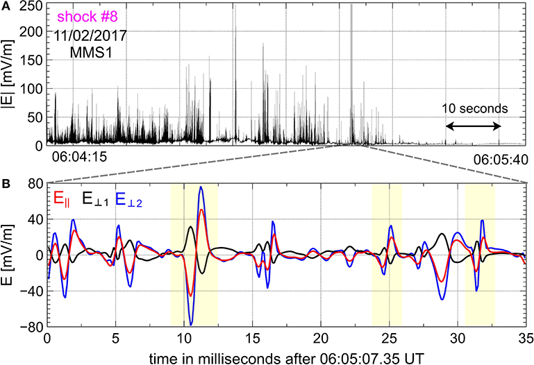
Figure 2. The electric field fluctuations measured at 8,192 S/s aboard MMS1 in shock #8: (A) the amplitude of the electric field fluctuations; (B) an expanded view of three electric field components measured over the 35 ms interval highlighted in (A). The electric field in (B) is in local magnetic field-aligned coordinates: E∥ is parallel to the local magnetic field, while E⊥1 and E⊥2 are perpendicular to the local magnetic field. (B) Demonstrates that some of the intense electric field fluctuations correspond to bipolar electrostatic structures. In this study the focus is on large-amplitude bipolar structures with electric field amplitudes exceeding 50 mV/m. In (B), the three highlighted bipolar structures are included in our dataset, while the other large-amplitude fluctuations with complicated profiles (unipolar, tripolar, or wave-packet) were not included in the dataset.
Figure 3 presents the analysis of a particular bipolar structure measured in shock #8. We consider voltage signals induced on voltage-sensitive probes by the electric field of the bipolar structure. Figures 3a,b plot the voltage signals V1 vs. −V2 and V3 vs. −V4 measured by two pairs of opposing probes on 60 m antennas in the spacecraft spin plane, while Figure 3c plots the voltage signals V5 vs. −V6 measured by two opposing probes on roughly 15 m antennas parallel to the spin axis. The noticeable correlations between the voltage signals of the opposing probes reflect the high quality of the electric field measurements [42]. Figure 3d presents components Eij of the electric field along the antenna directions computed using the voltage signals of the opposing probes, Eij ∝ (Vi − Vj)/2lij, with correction factors for the antenna frequency response and finite antenna length (see Vasko et al. [26] for the methodology), where l12 = l34 = 60 m and l56 = 14.6 m are antenna lengths. The bipolar profiles of the electric field components Eij indicate that the bipolar structure is essentially one-dimensional, while Figure 3e presents the dominant electric field El determined using minimum variance analysis [46]. The profiles of the electric field components Eij and the time delays between voltage signals measured by the opposing probes allow us to determine the sign of the electrostatic potential of the bipolar structure. The bipolar structure propagates from probe 1 to probe 2, while the electric field E12 is first negative and then positive. This implies that the electric field E12 has a convergent spatial configuration and, hence, the bipolar structure has to have a negative electrostatic potential. Similar analysis based on the other opposing probes consistently shows that the bipolar structure has a negative electrostatic potential.
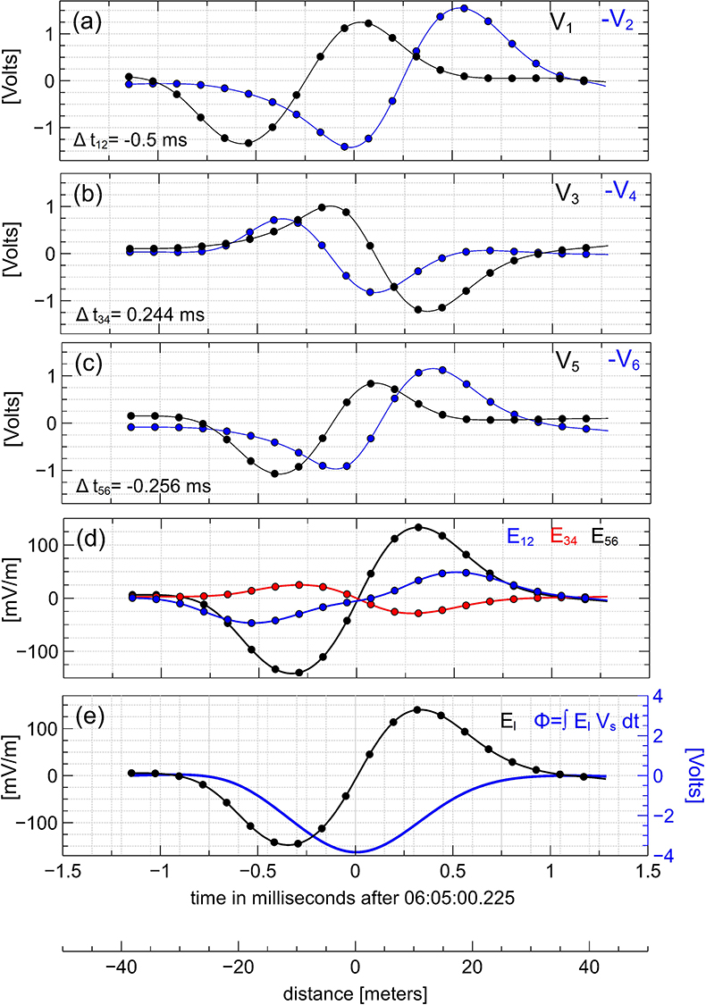
Figure 3. The interferometry analysis for a particular bipolar structure that was measured in shock #8 aboard MMS4. In all panels, the dots represent measured quantities, while the curves connecting them represent quantities upsampled using a spline interpolation. (a,b) Plot voltage signals V1 vs. −V2 and V3 vs. −V4 measured by two pairs of opposing probes in the spin plane, while (c) shows voltage signals V5 vs. −V6 of opposing probes on the spin axis. There is a clear correlation between each pair of voltage signals, which enables us to determine the time delays Δtij shown in the bottom left corners of (a–c). (d) Presents electric field components in the antenna coordinate system computed using voltage signals of the opposing probes: Eij ∝ (Vi − Vj)/2lij, where l12 = l34 = 60 m and l56 = 14.6 m; the similarity of the profiles of all three components implies that the bipolar structure is approximately one-dimensional. The time delays allow us to estimate the velocity Vs and direction of propagation of the bipolar structure as and kij = −VsΔtij/lij. We have found that Vs ≈ 50 km/s and k ≈ (0.43, −0.21, 0.88). By applying minimum variance analysis [46] to the electric fields Eij, we determine the dominant bipolar electric field El, which is presented in (e). Strong evidence for the bipolar structure being a one-dimensional structure is the small angle (of about 8°) between the electric field direction and the direction of propagation k. The electrostatic potential shown in (e) is computed using the upsampled El profile as Φ = ∫ElVsdt. The lowest horizontal axis shows the spatial distance ∫Vsdt measured from the time instant when El = 0.
The time delays Δtij between the voltage signals of the opposing probes are indicated in Figures 3a–c. We use the time delays to estimate the velocity Vs of the bipolar structure in the spacecraft frame, , and the direction k of propagation of the bipolar structure, kij = −VsΔtij/lij [the minus sign was missed in Vasko et al. [26] but did not affect their results]. We have found that the bipolar structure propagates with velocity Vs ≈ 50 km/s along vector k ≈ (0.43, −0.21, 0.88), which is within 8° of the electric field direction. The small angle between the electric field and the propagation direction is a strong indication that the bipolar structure is approximately a one-dimensional electrostatic structure. The estimated velocity allows us to translate temporal profiles into spatial profiles. Figure 3e shows that the spatial scale of the bipolar structure, determined as half the distance between minimum and maximum values of the electric field El, is l ≈ 17 m. Figure 3e presents the electrostatic potential of the bipolar structure, computed as Φ = ∫ElVsdt, and demonstrates that the amplitude of the electrostatic potential is Φ0 ≈ −3.8 V. In terms of the local Debye length λD and electron temperature Te, we have l ≈ 2λD and eΦ0 ≈ −0.15 Te, where e is the electron charge. This bipolar structure is similar to previously reported bipolar structures with negative electrostatic potentials in the Earth's bow shock [25–27].
The extensive dataset of bipolar structures that we collected allows us to detect bipolar structures with positive electrostatic potentials not reported previously. Figure 4 presents the analysis of one of these bipolar structures measured in shock #4. The noticeable correlations between the voltage signals of the opposing probes in Figures 4a–c indicate the high quality of the electric field measurements. Similar bipolar profiles of the electric field components Eij suggest that the bipolar structure should be approximately one-dimensional. The bipolar structure propagates from probe 2 to probe 1, while the electric field E12 is first negative and then positive. This implies that the electric field E12 has a divergent spatial configuration and, hence, the bipolar structure has to have a positive electrostatic potential. Analysis based on the other opposing probes consistently shows that the bipolar structure has a positive electrostatic potential. Using the time delays Δtij indicated in Figures 4a–c, we have found that the bipolar structure propagates with velocity Vs ≈ 45 km/s along direction k = (−0.37, 0.34, −0.86). The propagation direction is within 7° of the electric field direction, which is a strong indication that the bipolar structure is indeed a one-dimensional structure. Figure 4e shows that the spatial scale of the bipolar structure is l ≈ 25 m and the amplitude of the electrostatic potential is Φ0 ≈ 7 V. In terms of the local Debye length and electron temperature, we have l ≈ 4λD and eΦ0 ≈ 0.23 Te.
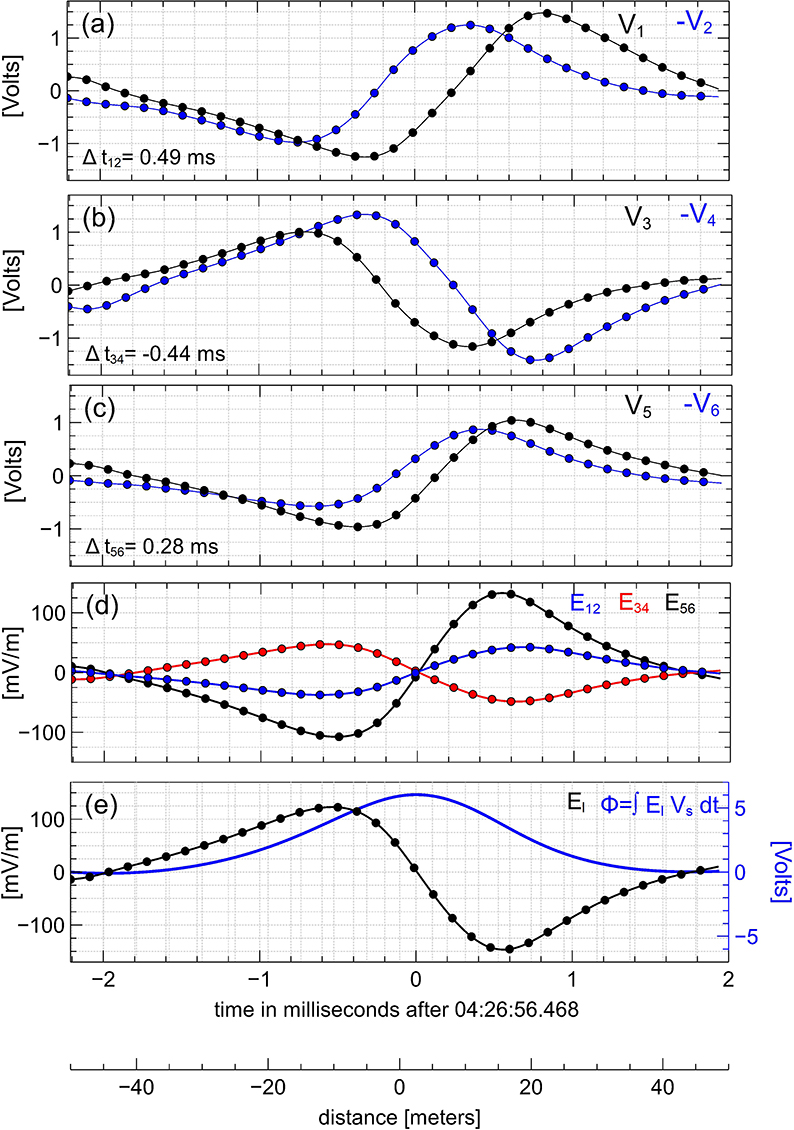
Figure 4. The interferometry analysis for a bipolar structure measured in shock #4 aboard MMS3. A distinct feature of the bipolar structure is that it has a positive electrostatic potential. The format of this figure is identical to that of Figure 3. The analysis shows that the bipolar structure propagates with velocity Vs ≈ 45 km/s along vector k = (−0.37, 0.34, −0.86), which is within 7° of the electric field direction.
The bipolar structures presented in Figures 3, 4 can be considered perfect in that all time delays between the voltage signals of the opposing probes could be well-determined. This is usually not the case for structures in the collected dataset, as demonstrated by a particular bipolar structure presented in Figure 5. Figures 5a–c show that the time delays can be well determined between the opposing probes in the spin plane, but not between the opposing probes on the spin axis. In addition, there are many bipolar structures in our dataset with time delays that are well determined only for one pair of the opposing probes. For bipolar structures such that at least one of the time delays is not well determined, we need to use a method of analysis different from the one described for bipolar structures in Figures 3, 4. Figures 3d, 4d shows that although the time delay between V5 and −V6 cannot be determined, the profile of the electric field E56 is bipolar and similar to the profiles of E12 and E34. In fact, the electric field components Eij always have similar bipolar profiles for the selected bipolar structures, which is a strong indication that the bipolar structures are approximately one-dimensional structures. Because the bipolar structures are electrostatic, we assume the propagation direction k to be parallel to the electric field direction determined by minimum variance analysis. We note that minimum variance analysis yields the electric field direction and, hence, the propagation direction k up to a sign chosen such that the velocity Vs is positive, and so the bipolar structure propagates parallel to the electric field direction. The velocity of propagation is estimated as Vs = −kijlij/Δtij, where ij is a pair of opposing probes with the best determined time delay Δtij. Whether a bipolar structure has a negative or a positive electrostatic potential is also determined using that pair of probes. In cases where time delays are well determined on two antennas, those antennas always provided consistent results on the sign of the electrostatic potential of a bipolar structure and similar estimates of the velocity Vs. In particular, the bipolar structure presented in Figure 5 has a positive electrostatic potential as inferred from both pairs of opposing probes in the spin plane and propagates with velocity Vs ≈ 85 km/s. Figure 5e shows that the bipolar structure has spatial scale l ≈ 20 m and amplitude of the electrostatic potential Φ0 ≈ 3 V. In terms of the local Debye length and electron temperature, we have l ≈ 2λD and eΦ0 ≈ 0.12 Te.
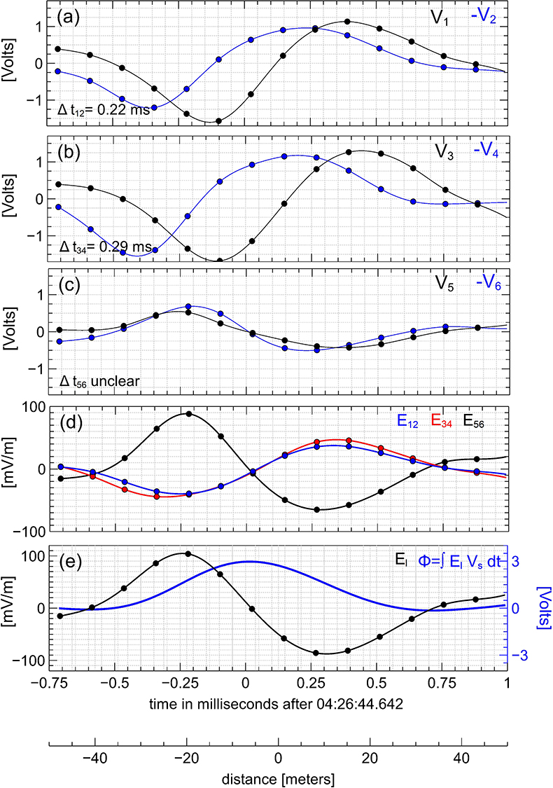
Figure 5. The interferometry analysis for a bipolar structure with a positive electrostatic potential that was measured in shock #4 aboard MMS3. The format of this figure is identical to that of Figure 3. The methodology used to determine the parameters of the bipolar structure is different from that for the bipolar structures in Figures 3, 4, because the time delay between voltage signals V5 and −V6 could not be well determined (see section 2 for details).
We have estimated the parameters of the selected bipolar structures using the interferometry method based on the antenna with the best determined time delay between voltage signals of the opposing probes. We have found that 361 of the bipolar structures have negative electrostatic potentials, while the remaining 10 have positive electrostatic potentials. In Figure 1, the occurrence of the bipolar structures is indicated along with the types of the bipolar structures, while Table 1 presents the numbers of bipolar structures with negative and positive potentials observed in each shock. The bipolar structures with positive potentials are observed in shocks #2, #3, #4, and #8; four of these structures are observed around shock ramps, while the other six occur in far-downstream regions. None of parameters MA, θBn, βe, i, and Te/Ti shown in Table 1 could be identified as being critical for the appearance of bipolar structures with positive electrostatic potentials.
Figure 6 presents a summary of the parameters of the bipolar structures. Figure 6a shows that the bipolar structures, whether they have positive and negative potentials, propagate with velocities from a few tens of km/s up to a few hundred km/s in the spacecraft frame, which is much smaller than the typical electron thermal velocity in the Earth's bow shock. Typical amplitudes |Φ0| of the bipolar structures are a few volts, though they can be up to 30 V. Figure 6b shows that in terms of local electron temperature, the bipolar structures typically have amplitudes of |eΦ0| ≲ 0.1 Te, though these can be as large as 0.5 Te. Typical spatial scales of the bipolar structures are a few λD, though they can be up to about 10λD. There is a noticeable positive correlation between |eΦ0|/Te and l/λD, whose physical nature will be clarified in the next section. Figures 6a,b demonstrate that velocities, spatial scales and absolute amplitudes of the bipolar structures with positive and negative potentials are basically similar.
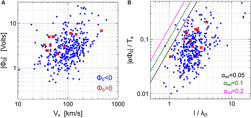
Figure 6. The results of the statistical analysis of 371 bipolar electrostatic structures: (A) the absolute amplitude |Φ0| of the electrostatic potential vs. the velocity of propagation Vs in the spacecraft frame; (B) |eΦ0|/Te vs. l/λD, where Te and λD are the local electron temperature and Debye length, and l is the spatial scale of a bipolar structure. The blue and red crosses correspond to bipolar structures with negative and positive electrostatic potentials, respectively. The dashed curves in (B) represent upper estimates of the amplitudes of ion phase space holes produced by the two-stream instability between incoming and reflected ions. The upper estimates are given by Equation (3), with αref being the fraction of incoming ions reflected to the upstream region. The upper estimates are demonstrated for typical values of the fraction of reflected ions in the Earth's bow shock (e.g., Leroy et al. [47]).
3. Theoretical Interpretation
The bipolar electrostatic structures with negative potentials are most likely ion phase space holes, which are coherent structures formed in a nonlinear stage of various ion streaming instabilities [31, 48–50]. Interestingly, very early numerical simulations showed that ion streaming instabilities can potentially produce Debye-scale electrostatic structures with negative potentials in the Earth's bow shock [51, 52]. In the linear stage of an ion streaming instability, electrostatic fluctuations grow at the expense of the energy of resonant ions. In a nonlinear stage, the amplitude of the electrostatic fluctuations becomes sufficiently large to trap a fraction of resonant ions into potential wells of the electrostatic fluctuations, resulting in the formation of vortices in the ion phase space. The merging of these vortices leads to formation of electrostatic solitary waves called ion phase space holes [48, 49].
Although the details of ion velocity distribution functions, whose instability results in formation of ion phase space holes in the Earth's bow shock, are not known, we can estimate the growth rates of that instability. The instability saturates when the bounce frequency of ions trapped within electrostatic fluctuations becomes comparable to the initial increment of the instability [53]. Therefore, the initial increment γ should be of the order of the bounce frequency of ions trapped within the observed bipolar structures, . This condition can be written as
where ωpi is the ion plasma frequency. Adopting typical parameters of the bipolar structures (Figure 6), we find initial increments on the order of a fraction of the ion plasma frequency, γ ~ 0.1 ωpi. In supercritical shocks, increments of that order can in principle be provided by the two-stream instability between incoming and reflected ions. The maximum growth rate of ion-acoustic waves driven by that instability is reached when both incoming and reflected ions are cold [34, 54]: , where αref is the fraction of incoming ions reflected to the upstream region and has a typical value of 0.1 in the Earth's bow shock [47]. Equation (1) can be written as
which explains the positive correlation between the amplitude and spatial scale of the bipolar structures noticeable in Figure 6b. Because at finite temperatures of incoming and reflected ions the increment of the two-stream instability γ is smaller than γmax [55], we can give the following upper estimate for the amplitudes of the bipolar structures:
Figure 6b demonstrates that the amplitudes of the bipolar structures are indeed below the upper estimate for typical fractions αref of reflected ions.
Direct identification of the ion two-stream instability using measurements of the ion velocity distribution function in the Earth's bow shock is expected to be complicated. The observed parameters of the bipolar structures indicate that the inverse bounce frequency of trapped ions is of the order of one millisecond. The relaxation of ion beams seeding the formation of ion phase space holes is expected to occur on a time scale of a few tens of inverse bounce periods [53], while ion velocity distribution functions aboard MMS are available at a 0.15 s cadence. Therefore, the measured ion velocity distribution functions are expected to correspond to a marginally stable relaxed state. The fast relaxation of the ion velocity distribution function explains the results of the stability analysis of Goodrich et al. [56], who demonstrated that measured ion velocity distribution functions are stable with respect to simultaneously measured ion-acoustic waves. An alternative approach to identifying the nature of an instability seeding the formation of ion phase space holes is based on analysis and comparison of the properties of these bipolar structures to predictions of a particular instability. Wang et al. [27] have suggested that approach and provided strong arguments in favor of the ion two-stream instability as the source of bipolar structures with negative potentials.
The analysis in section 2 showed that in addition to bipolar structures with negative potentials, there are bipolar structures with positive potentials, albeit in negligible numbers. The bipolar structures with positive potentials can be electron phase space holes [31, 32] produced by various electron streaming instabilities, which are expected to operate in the transition region of the Earth's bow shock [57, 58]. In terms of parameters, these bipolar structures are similar to slow electron phase space holes observed in reconnection current sheets [59, 60] and the plasma sheet boundary layer [61] in the Earth's magnetosphere. The bump-on-tail instability cannot be a source of these bipolar structures, because in that case the bipolar structures would propagate with velocities that are a fraction of the electron thermal velocity [57, 62]. Instabilities capable of producing slow electron phase space holes include the electron two-stream instability [58, 62, 63] and the Buneman instability [64, 65], though the latter is less likely to operate under conditions typical of the Earth's bow shock. Whichever instability potentially produces the bipolar structures with positive potentials, the initial increment should be on the order of the bounce frequency of electrons trapped within the bipolar electric field:
where ωpe is the electron plasma frequency. Adopting typical parameters of the bipolar structures (Figure 6), we find initial increments that are a fraction of the electron plasma frequency, γ ~ 0.1 ωpe. Increments of this magnitude can in principle be provided by the electron two-stream instability [58]. Although the bipolar structures with positive potentials can be electron phase space holes, we note the alternative interpretation of these bipolar structures in terms of ion-acoustic solitons arising from ion-acoustic fluctuations due to electron and ion fluid nonlinearities [66, 67]. The detailed analysis of this alternative interpretation is left for a separate study.
The critical result of the statistical analysis in section 2 is that only 10 out of 371 bipolar structures, accounting for <3% of the structures, have positive potentials and can be interpreted in terms of electron phase space holes. Does the scarcity of bipolar structures with positive potentials imply that electron streaming instabilities rarely operate in the Earth's bow shock, or that the formation of these structures is hindered in conditions typical of the Earth's bow shock? We lean toward the second scenario. According to existing simulation and theoretical studies [36, 37], one-dimensional electron phase space holes can be stable with respect to the transverse instability only under the condition that the bounce frequency of trapped electrons should be smaller than the electron cyclotron frequency, ωb ≲ ωce. This stability criterion can be written in the form of an upper estimate for electron hole amplitudes:
With realistic background parameters, ωpe/ωce ~ 100, an electron phase space hole with the spatial scale of a few Debye lengths can be stable with respect to the transverse instability, provided that , which implies Φ0 ≲ 0.01 V, where we have assumed that by the order of magnitude Te ~ 10 eV. Taking into account that a few Debye lengths is a few tens of meters, we find that electron phase space holes can be stable with respect to the transverse instability provided that the electric field amplitude is rather small, E ≲ 1 mV/m. Electron phase space holes with electric field amplitudes larger than about 1 mV/m should be rarely observed in the Earth's bow shock because of the transverse instability. Thus, the transverse instability may explain the observed scarcity of bipolar structures with positive potentials among large-amplitude bipolar structures in the Earth's bow shock.
4. Discussion and Conclusion
We have presented statistical analysis of large-amplitude bipolar electrostatic structures measured in the Earth's bow shock by Magnetospheric Multiscale spacecraft. We have found that over 97% of the bipolar structures in the Earth's bow shock have negative potentials. We have interpreted these bipolar structures in terms of ion phase space holes and obtained an upper estimate for the amplitude of these structures. The copious amount of ion phase space holes in the Earth's bow shock is a strong indication that ion streaming instabilities, and in particular the two-stream instability between incoming and reflected ions, drive electrostatic fluctuations in the Earth's bow shock. The statistical analysis has also shown that <3% of the bipolar structures have positive potentials and that these can in principle be interpreted in terms of electron phase space holes. The observed rarity of bipolar structures with positive potentials may be due to the transverse instability of electron phase space holes, the criterion for which is strongly dependent on ωpe/ωce.
The results presented here imply that the efficiency of the electron surfing acceleration mechanism originally demonstrated in 1D Particle-In-Cell simulations of high-Mach-number shocks [10, 11] will be restricted. In the surfing acceleration mechanism, electron phase space holes appearing in a nonlinear stage of the Buneman instability operating in the shock transition region facilitate prolonged trapping of electrons around the shock ramp, resulting in efficient electron acceleration by the motional electric field. We note that the transverse instability of electron phase space holes is suppressed in one-dimensional simulations, because that instability is a multi-dimensional effect [36, 37]. In one-dimensional simulations, electron phase space holes are generally stable over an indefinitely long time at any ωpe/ωce [62, 63]. In realistic three-dimensional shocks and under realistic background plasma parameters, ωpe/ωce ≫ 1, the transverse instability of electron phase space holes will strongly reduce the efficiency of electron acceleration via the original surfing acceleration mechanism. Thus, our analysis of large-amplitude bipolar structures in the Earth's bow shock has demonstrated that the surfing acceleration mechanism involving electron phase space holes is highly unlikely to be efficient in realistic collisionless shocks. The stochastic surfing acceleration mechanism is a prospective mechanism, though, because it does not require the presence of coherent electrostatic structures [9, 12].
Data Availability Statement
The MMS data used in the analysis are publicly available at https://lasp.colorado.edu/mms/public.
Author Contributions
IV and RW performed the MMS data analysis and wrote the manuscript. FM contributed to the interpretation of the electric field measurements. IV, SB, and AA contributed to the theoretical interpretation.
Funding
This work was supported by the NASA MMS Guest Investigator grant No. 80NSSC18K0155. IV thanks the International Space Science Institute (ISSI), Bern, Switzerland, for support. AA was supported by the Russian Science Foundation grant No. 19-12-00313.
Conflict of Interest
The authors declare that the research was conducted in the absence of any commercial or financial relationships that could be construed as a potential conflict of interest.
Acknowledgments
We thank the MMS teams for the excellent data, which are publicly available at https://lasp.colorado.edu/mms/public. IV is grateful for discussions with Vladimir Krasnoselskikh and members of the ISSI team on Resolving the Microphysics of Collisionless Shock Waves (http://www.issibern.ch/teams/collisionlesshockwave/).
Footnotes
1. ^The website https://cdaweb.gsfc.nasa.gov/ provides Wind spacecraft measurements of plasma parameters at 1 min cadence time-shifted to the nose of the Earth's bow shock. A time-shift that is of the order of one hour takes into account solar wind propagation from the Wind spacecraft to the nose of the Earth's bow shock.
References
1. Kennel CF, Edmiston JP, Hada T. A quarter century of collisionless shock research. In: Stone RG, Tsurutani BT, editors. Collisionless Shocks in the Heliosphere. A Tutorial Review. Washington, DC: American Geophysical Union (1985). p. 1–36.
2. Papadopoulos K. Microinstabilities and anomalous transport. In: Stone RG, Tsurutani BT, editors. Collisionless Shocks in the Heliosphere. A Tutorial Review. Washington, DC: American Geophysical Union (1985). p. 59–90.
3. Krasnoselskikh V, Balikhin M, Walker SN, Schwartz S, Sundkvist D, Lobzin V, et al. The dynamic quasiperpendicular shock: cluster discoveries. Space Sci Rev. (2013) 178:535–98. doi: 10.1007/s11214-013-9972-y
4. Bale SD, Mozer FS. Measurement of large parallel and perpendicular electric fields on electron spatial scales in the terrestrial bow shock. Phys Rev Lett. (2007) 98:205001. doi: 10.1103/PhysRevLett.98.205001
5. Mozer FS, Sundkvist D. Electron demagnetization and heating in quasi-perpendicular shocks. J Geophys Res. (2013) 118:5415–20. doi: 10.1002/jgra.50534
6. Wilson LB, Sibeck DG, Breneman AW, Le Contel O, Cully C, Turner DL, et al. Quantified energy dissipation rates in the terrestrial bow shock: 2. Waves and dissipation. J Geophys Res. (2014) 119:6475–95. doi: 10.1002/2014JA019930
7. Papadopoulos K. Electron heating in superhigh mach number shocks. Astrophys Space Sci. (1988) 144:535–47. doi: 10.1007/BF00793203
8. Shimada N, Hoshino M. Electron heating and acceleration in the shock transition region: background plasma parameter dependence. Phys Plasmas. (2004) 11:1840–9. doi: 10.1063/1.1652060
9. Matsumoto Y, Amano T, Hoshino M. Electron accelerations at high mach number shocks: two-dimensional particle-in-cell simulations in various parameter regimes. Astphys J. (2012) 755:109. doi: 10.1088/0004-637X/755/2/109
10. Hoshino M, Shimada N. Nonthermal electrons at high mach number shocks: electron shock surfing acceleration. Astphys J. (2002) 572:880–7. doi: 10.1086/340454
11. Schmitz H, Chapman SC, Dendy RO. Electron preacceleration mechanisms in the foot region of high Alfvénic mach number shocks. Astphys J. (2002) 579:327–36. doi: 10.1086/341733
12. Amano T, Hoshino M. Electron shock surfing acceleration in multidimensions: two-dimensional particle-in-cell simulation of collisionless perpendicular shock. Astphys J. (2009) 690:244–51. doi: 10.1088/0004-637X/690/1/244
13. Umeda T, Yamao M, Yamazaki R. Electron acceleration at a low mach number perpendicular collisionless shock. Astphys J. (2009) 695:574–9. doi: 10.1088/0004-637X/695/1/574
14. Troland TH, Heiles C. Interstellar magnetic field strengths and gas densities: observational and theoretical perspectives. Astphys J. (1986) 301:339. doi: 10.1086/163904
15. Comişel H. On electron adiabaticity in collisionless shocks. Front Phys. (2016) 4:29. doi: 10.3389/fphy.2016.00029
16. Fredricks RW, Coroniti FV, Kennel CF, Scarf FL. Fast time-resolved spectra of electrostatic turbulence in the earth's bow shock. Phys Rev Lett. (1970) 24:994–8. doi: 10.1103/PhysRevLett.24.994
17. Rodriguez P, Gurnett DA. Correlation of bow shock plasma wave turbulence with solar wind parameters. J Geophys Res. (1976) 81:2871. doi: 10.1029/JA081i016p02871
18. Formisano V, Torbert R. Ion acoustic wave forms generated by ion-ion streams at the Earth's bow shock. Geophys Res Lett. (1982) 9:207–10. doi: 10.1029/GL009i003p00207
19. Balikhin M, Walker S, Treumann R, Alleyne H, Krasnoselskikh V, Gedalin M, et al. Ion sound wave packets at the quasiperpendicular shock front. Geophys Res Lett. (2005) 32:L24106. doi: 10.1029/2005GL024660
20. Hull AJ, Larson DE, Wilber M, Scudder JD, Mozer FS, Russell CT, et al. Large-amplitude electrostatic waves associated with magnetic ramp substructure at Earth's bow shock. Geophys Res Lett. (2006) 33:L15104. doi: 10.1029/2005GL025564
21. Goodrich KA, Ergun R, Schwartz SJ, Wilson LB, Newman D, Wilder FD, et al. MMS observations of electrostatic waves in an oblique shock crossing. J Geophys Res. (2018) 123:9430–42. doi: 10.1029/2018JA025830
22. Matsumoto H, Kojima H, Kasaba Y, Miyake T, Anderson R, Mukai T. Plasma waves in the upstream and bow shock regions observed by geotail. Adv Space Res. (1997) 20:683–93. doi: 10.1016/S0273-1177(97)00456-0
23. Bale SD, Kellogg PJ, Larsen DE, Lin RP, Goetz K, Lepping RP. Bipolar electrostatic structures in the shock transition region: evidence of electron phase space holes. Geophys Res Lett. (1998) 25:2929–32. doi: 10.1029/98GL02111
24. Bale SD, Hull A, Larson DE, Lin RP, Muschietti L, Kellogg PJ, et al. Electrostatic turbulence and debye-scale structures associated with electron thermalization at collisionless shocks. Astphys J Lett. (2002) 575:L25–8. doi: 10.1086/342609
25. Hobara Y, Walker SN, Balikhin M, Pokhotelov OA, Gedalin M, Krasnoselskikh V, et al. Cluster observations of electrostatic solitary waves near the Earth's bow shock. J Geophys Res. (2008) 113:A05211. doi: 10.1029/2007JA012789
26. Vasko IY, Mozer FS, Krasnoselskikh VV, Artemyev AV, Agapitov OV, Bale SD, et al. Solitary waves across supercritical quasi-perpendicular shocks. Geophys Res Lett. (2018) 45:5809–17. doi: 10.1029/2018GL077835
27. Wang R, Vasko IY, Mozer FS, Bale SD, Artemyev AV, Bonnell JW, et al. Electrostatic turbulence and Debye-scale structures in collisionless shocks. Astphys J Lett. (2020) 889:L9. doi: 10.3847/2041-8213/ab6582
28. Breneman AW, Cattell CA, Kersten K, Paradise A, Schreiner S, Kellogg PJ, et al. STEREO and wind observations of intense cyclotron harmonic waves at the Earth's bow shock and inside the magnetosheath. J Geophys Res. (2013) 118:7654–64. doi: 10.1002/2013JA019372
29. Walker SN, Balikhin MA, Alleyne HSCK, Hobara Y, André M, Dunlop MW. Lower hybrid waves at the shock front: a reassessment. Ann Geophys. (2008) 26:699–707. doi: 10.5194/angeo-26-699-2008
30. Fuselier SA, Gurnett DA. Short wavelength ion waves upstream of the earth's bow shock. J Geophys Res. (1984) 89:91–104. doi: 10.1029/JA089iA01p00091
31. Schamel H. Electron holes, ion holes and double layers. Electrostatic phase space structures in theory and experiment. Phys Rep. (1986) 140:161–91. doi: 10.1016/0370-1573(86)90043-8
32. Hutchinson IH. Electron holes in phase space: what they are and why they matter. Phys Plasmas. (2017) 24:055601. doi: 10.1063/1.4976854
33. Mozer FS, Agapitov OV, Giles B, Vasko I. Direct observation of electron distributions inside millisecond duration electron holes. Phys Rev Lett. (2018) 121:135102. doi: 10.1103/PhysRevLett.121.135102
34. Akimoto K, Winske D. Ion-acoustic-like waves excited by the reflected ions at the earth's bow shock. J Geophys Res. (1985) 90:12095–103. doi: 10.1029/JA090iA12p12095
35. Fuselier SA, Gary PS, Thomsen MF, Bame SJ, Gurnett DA. Ion beams and the ion/ion acoustic instability upstream from the Earth's bow shock. J Geophys Res. (1987) 92:4740–4. doi: 10.1029/JA092iA05p04740
36. Muschietti L, Roth I, Carlson CW, Ergun RE. Transverse instability of magnetized electron holes. Phys Rev Lett. (2000) 85:94–7. doi: 10.1103/PhysRevLett.85.94
37. Hutchinson IH. Transverse instability magnetic field thresholds of electron phase-space holes. Phys Rev E. (2019) 99:053209. doi: 10.1103/PhysRevE.99.053209
38. Russell CT, Anderson BJ, Baumjohann W, Bromund KR, Dearborn D, Fischer D, et al. The magnetospheric multiscale magnetometers. Space Sci Rev. (2016) 199:189–256. doi: 10.1007/s11214-014-0057-3
39. Ergun RE, Tucker S, Westfall J, Goodrich KA, Malaspina DM, Summers D, et al. The axial double probe and fields signal processing for the MMS mission. Space Sci Rev. (2016) 199:167–88. doi: 10.1007/s11214-014-0115-x
40. Lindqvist PA, Olsson G, Torbert RB, King B, Granoff M, Rau D, et al. The spin-plane double probe electric field instrument for MMS. Space Sci Rev. (2016) 199:137–65. doi: 10.1007/s11214-014-0116-9
41. Pollock C, Moore T, Jacques A, Burch J, Gliese U, Saito Y, et al. Fast plasma investigation for magnetospheric multiscale. Space Sci Rev. (2016) 199:331–406. doi: 10.1007/s11214-016-0245-4
42. Mozer FS. DC and low-frequency double probe electric field measurements in space. J Geophys Res. (2016) 121:10. doi: 10.1002/2016JA022952
43. Scudder JD. A review of the physics of electron heating at collisionless shocks. Adv Space Res. (1995) 15:181–223. doi: 10.1016/0273-1177(94)00101-6
44. Schwartz SJ, Henley E, Mitchell J, Krasnoselskikh V. Electron temperature gradient scale at collisionless shocks. Phys Rev Lett. (2011) 107:215002. doi: 10.1103/PhysRevLett.107.215002
45. Vinas AF, Scudder JD. Fast and optimal solution to the ‘Rankine-Hugoniot problem’. J Geophys Res. (1986) 91:39–58. doi: 10.1029/JA091iA01p00039
46. Sonnerup BUÖ, Scheible M. Minimum and maximum variance analysis. In: Paschmann G, Dal P, editors. Analysis Methods for Multi-Spacecraft Data. ISSI Scientific Reports Series. Noordwijk: ESA Publications Division (1998). p. 185–220.
47. Leroy MM, Winske D, Goodrich CC, Wu CS, Papadopoulos K. The structure of perpendicular bow shocks. J Geophys Res. (1982) 87:5081–94. doi: 10.1029/JA087iA07p05081
48. Kofoed-Hansen O, Pecseli HL, Trulsen J. Coherent structures in numerically simulated plasma turbulence. Phys Scripta. (1989) 40:280–94. doi: 10.1088/0031-8949/40/3/004
49. Børve S, Pécseli HL, Trulsen J. Ion phase-space vortices in 2.5-dimensional simulations. J Plasma Phys. (2001) 65:107–29. doi: 10.1017/S0022377801008947
50. Goldman MV, Newman DL, Ergun RE. Phase-space holes due to electron and ion beams accelerated by a current-driven potential ramp. Nonlin Process Geophys. (2003) 10:37–44. doi: 10.5194/npg-10-37-2003
51. Papadopoulos K. Ion thermalization in the Earth's bow shock. J Geophys Res. (1971) 76:3806. doi: 10.1029/JA076i016p03806
52. Biskamp D, Welter H. Structure of the Earth's bow shock. J Geophys Res. (1972) 77:6052. doi: 10.1029/JA077i031p06052
54. Ohira Y, Takahara F. Oblique ion two-stream instability in the foot region of a collisionless shock. Astphys J. (2008) 688:320–6. doi: 10.1086/592182
55. Gary SP, Omidi N. The ion-ion acoustic instability. J Plasma Phys. (1987) 37:45–61. doi: 10.1017/S0022377800011983
56. Goodrich KA, Ergun R, Schwartz SJ, Wilson LB, Johlander A, Newman D, et al. Impulsively reflected ions: a plausible mechanism for ion acoustic wave growth in collisionless shocks. J Geophys Res. (2019) 124:1855–65. doi: 10.1029/2018JA026436
57. Thomsen MF, Barr HC, Gary SP, Feldman WC, Cole TE. Stability of electron distributions within the earth's bow shock. J Geophys Res. (1983) 88:3035–45. doi: 10.1029/JA088iA04p03035
58. Gedalin M. Two-stream instability of electrons in the shock front. Geophys Res Lett. (1999) 26:1239–42. doi: 10.1029/1999GL900239
59. Khotyaintsev YV, Vaivads A, André M, Fujimoto M, Retinò A, Owen CJ. Observations of slow electron holes at a magnetic reconnection site. Phys Rev Lett. (2010) 105:165002. doi: 10.1103/PhysRevLett.105.165002
60. Graham DB, Khotyaintsev YV, Vaivads A, André M. Electrostatic solitary waves and electrostatic waves at the magnetopause. J Geophys Res. (2016) 121:3069–92. doi: 10.1002/2015JA021527
61. Norgren C, André M, Vaivads A, Khotyaintsev YV. Slow electron phase space holes: magnetotail observations. Geophys Res Lett. (2015) 42:1654–61. doi: 10.1002/2015GL063218
62. Omura Y, Matsumoto H, Miyake T, Kojima H. Electron beam instabilities as generation mechanism of electrostatic solitary waves in the magnetotail. J Geophys Res. (1996) 101:2685–98. doi: 10.1029/95JA03145
63. Morse RL, Nielson CW. One-, two-, and three-dimensional numerical simulation of two-beam plasmas. Phys Rev Lett. (1969) 23:1087–90. doi: 10.1103/PhysRevLett.23.1087
64. Buneman O. Instability, turbulence, and conductivity in current-carrying plasma. Phys Rev Lett. (1958) 1:8–9. doi: 10.1103/PhysRevLett.1.8
65. Norgren C, André M, Graham, D. B., Khotyaintsev, Yu. V. Vaivads, A. Slow electron holes in multicomponent plasmas. Geophys Res Lett. (2015) 42:7264–72. doi: 10.1002/2015GL065390
Keywords: collisionless shocks, electrostatic turbulence, bipolar electrostatic structures, ion holes, electron holes, surfing acceleration
Citation: Vasko IY, Wang R, Mozer FS, Bale SD and Artemyev AV (2020) On the Nature and Origin of Bipolar Electrostatic Structures in the Earth's Bow Shock. Front. Phys. 8:156. doi: 10.3389/fphy.2020.00156
Received: 23 December 2019; Accepted: 15 April 2020;
Published: 12 June 2020.
Edited by:
Michael Gedalin, Ben-Gurion University of the Negev, IsraelReviewed by:
Octav Marghitu, Space Science Institute, RomaniaNickolay Ivchenko, Royal Institute of Technology, Sweden
Copyright © 2020 Vasko, Wang, Mozer, Bale and Artemyev. This is an open-access article distributed under the terms of the Creative Commons Attribution License (CC BY). The use, distribution or reproduction in other forums is permitted, provided the original author(s) and the copyright owner(s) are credited and that the original publication in this journal is cited, in accordance with accepted academic practice. No use, distribution or reproduction is permitted which does not comply with these terms.
*Correspondence: Ivan Y. Vasko, aXZhbi52YXNrb0Bzc2wuYmVya2VsZXkuZWR1