Adaptive Neural Network Control of Chaotic Fractional-Order Permanent Magnet Synchronous Motors Using Backstepping Technique

The backstepping technique is greatly effective for the integer-order triangular non-linear systems. Nevertheless, it is dramatically challenging to implement backstepping technique in the manipulation of fractional-order permanent magnet synchronous motors (FOPMSMs), since the fractional derivatives of the composite functions are deeply complex. In this paper, adaptive neural network (NN) backstepping-based control scheme for FOPMSMs on the basis of fractional Lyapunov stability criterion is established. First, we propose a novel adaptive synchronous controller for FOPMSMs by coupling with NNs and backstepping technique. Then, we present a detailed stability analysis in terms of FOPMSMs via the proposed controller. Finally, a simulation example is given to reveal that the proposed controller can effectively eliminate or restrain the chaos of FOPMSMs, and keep the tracking signals synchronous with the reference signals.

1. Introduction

In late decades, fractional-order non-linear systems (FONSs) [1] have been widely studied, not only owing to their accurate performance in modeling physical phenomena (e.g., chaos, oscillations, impulses, diffusions, see [2–5]), but also owing to their successful applications in a variety of fields, such as chemistry, medicine, biology, electronics, robotics, fuel cells, and so on [6–11]. Stability analysis [12] is regarded as a fundamental and crucial task in the development of cybernetics. Recently, more and more scholars have paid attention to stability analysis of fractional-order non-linear systems [13–16]. It is not exaggerated to say that stability analysis of FONSs along with their robust control have become a hot and promising research topic.

The researches on the control of chaotic systems are widely concerned due to its valuable significance in both theoretical and practical aspects [17, 18]. Since Kuroe and Hayashi [19] originally discovered chaotic phenomenon from the motor drive system in the late 1980's, chaos control has been one of the most popular research topics in cybernetics. There are several types of chaotic motor drivers that capture widespread interests. For instance, DC motor drivers [20], step motor drivers [21], single-phase induction motor drivers [22], synchronous reluctance motor drivers [23], switched reluctance motor drivers [24] and so on. The extensive utilization of permanent magnet synchronous motors (PMSMs) in industries mainly benefits from their merits of high speed, high efficiency, high power, low loss and low temperature rise. Chaotic non-linear systems are very complex due to the irregular and unpredictable behaviors. A remarkable feature of chaotic systems is that they are very sensitive to the initial conditions. The small change of initial state will lead to great distinction. On the other hand, they have many other desired properties, such as information processing, secure communication and mechanical system. However, it may cause unexpected oscillations and even destroy the system stability. Therefore, such oscillations should be effectively suppressed. For this reason, various methods have been developed to stabilize non-linear chaotic systems, in which fractional order chaos control has also been focused, such as OGY type [25], feedback type [26–28], dynamic surface type [29], sliding mode type [30–33], backstepping type [34, 35], etc.

Neural network (NN) control technique [36, 37] is an intelligent method for controlling non-linear systems with uncertainties. Analogizing to fuzzy control approach [38, 39], the idea of NN control technique is to approximate unknown non-linear functions by using radial basis function neural networks (RBFNNs), which is a type of neuron-modeled structure formed by the computation of some adjustable parameter vectors and some specific continuous functions. As one of the most powerful tools to realizing approximation of functions, NN control technique is popular because it facilitates to control most of many non-linear systems in which the data are too imprecise or too complex to construct mathematical modeling. It provides an available way for the control designs, and it is considerably applicable in the field of control engineering.

Backstepping technique has engaged much attention due to its efficient performance in handling mismatched uncertainties of integer-order non-linear systems [40, 41]. Unfortunately, this control method has an inherent drawback, namely “explosion of complexity,” triggered by iteratively differentiating virtual control inputs [42]. Additionally, it requires complicated analysis to compute a so-called “regression matrix” [43]. Dawson et al. [44] pointed out that the size of the regression matrix displays too large when backstepping technique was applied to manipulate DC motors in a conventional manner. Such complexities might be augmented remarkably for fractional-order non-linear systems.

It is well-known that the design of NN control is rarely systematic, which is difficult to work for the control of complex systems. It is also challenging to establish a systematic NN control theory to solve a series of problems, such as the mechanism of NN control, stability analysis, systematic design, etc. Backstepping control usually leads to the problem of “complexity explosion” when it is applied in the processing of unknown functions, so the methods of adaptive NN control [36], adaptive fuzzy control [45] and adaptive NN backstepping control [35] are put forward to address such a problem. These techniques enable systems to be greatly adaptive and robust obeying the required performance criteria for the control. However, the control performance is not desired for the non-linear systems with triangular structures, and the problem of “complexity explosion” will occur during the control proceeding. Based on the above discussion, this paper proposes an adaptive neural network control method of chaotic fractional-order permanent magnet synchronous motors using backstepping technique, which can improve the control performance of non-linear systems.

To deal with the synchronization issue of fractional-order permanent magnet synchronous motor (FOPMSM) with triangular structure, we expect to construct an adaptive NN controller combined with backstepping technique. This enables every uncertain complex non-linear functions being approximated by a radial basis function neural network (RBFNN) during each control step. The main contributions of this work can be summarized as follows:

The synchronization control scheme design and the stability analysis of FOPMSMs are investigated. In order to analyze the stability of the controlled systems, firstly, some basic results related to fractional calculus and RBFNN are recalled, including a fractional differential inequality, which lays the foundation for the application of the fractional Lyapunov function method. Meanwhile, it lays a foundation for the stability analysis of other types of FONSs. Secondly, an adaptive NN backstepping recursive control method is proposed for a class of uncertain FOPMSMs. The stability of FOPMSMs is analyzed based on fractional Lyapunov criterion. NN control technique is employed when dealing with the approximation of uncertain functions of FOPMSMs, and the fractional adaptive law is designed to update the parameters of NNs. The relevant properties of Mittag-Leffler function and Laplace transform are applied when the fractional Lyapunov function is defined to implement the system control. Our proposed control method fully averts the superfluous terms which are aroused by repeated derivation on virtual control inputs, and facilitates to overcome the so-called “complexity explosion” inherent drawback of the traditional backstepping technique. Finally, we present a numerical example to verify the main results. The simulation results show that our method embodies a perfect control effect. This also reveals the effectiveness of our control algorithm in another way.

The remainder of this work is arranged as below: In section 2, we recall several fundamental preliminaries of fractional calculus and RBFNN. Then, a brief overview of a class of FOPMSMs is provided. In section 3, we propose a RBFNN-based control scheme in three steps and present stability analysis. In section 4, we illustrate the effectiveness of the proposed synchronous controller via a simulation example. Finally, in section 5, we summarize the results of this work and put forward the prospect for our further investigation.

2. Preliminaries and Model Description

Some basic concepts, notations and lemmas, involved with fractional calculus and radial basis function neural network (RBFNN), need to be stated in this section before used. For convenience, we adopt the symbol ℝ (resp. ℝⁿ, ℂ) to represent the collection of all real numbers (resp. n-dimensional real vectors, complex numbers). Ω ⊆ ℝⁿ is always assumed to be compact. T = [0, +∞) means the time-variable domain. The notation C¹(T, Ω) stands for the collection of all continuous functions from T to Ω with continuous derivatives. Given a vector x ∈ ℝⁿ, x^T denotes its transpose, ∥x∥ denotes its Euclidean norm.

Definition 1 ([8]). Let α ≥ 0. For a given function f :[0, ∞) → ℝ, its α-th order integral is written as

$\begin{array}{ll}{{}_0{I}}_{\psi }^{\alpha }f(\psi )=\frac{1}{\Gamma (\alpha )}{\displaystyle {\int }_0^{\psi }}\frac{f(\eta )}{{(\psi -\eta )}^{1-\alpha }}\text{d}\eta ,\psi >0& (1)\end{array}$

where $\Gamma (\alpha )={\int }_0^{+\infty }{s}^{\alpha -1}{e}^{-s}\text{d}s$.

Definition 2 ([8]). Let α ≥ 0. For a given function f :[0, ∞) → ℝ, its α-th order Caputo derivative is expressed by

$\begin{array}{ll}{{}_0{}^C{D}}_{\psi }^{\alpha }f(\psi )=\frac{1}{\Gamma (n-\alpha )}{\displaystyle {\int }_0^t}\frac{f^{(n)}(\eta )}{{(\psi -\eta )}^{\alpha +1-n}}\text{d}\eta ,\alpha \ge 0,\psi >0& (2)\end{array}$

where α ∈ [n − 1, n), n = 1, 2, ⋯ .

Definition 3 ([8]). Let α, γ > 0. The Mittag-Leffler function E_α,γ on ℂ is expressed as

$\begin{array}{ll}{E}_{\alpha ,\gamma }(\zeta )={\displaystyle \sum _{k=0}^{\infty }}\frac{{\zeta }^k}{\Gamma (\alpha k+\gamma )}.& (3)\end{array}$

Moreover, taking the Laplace transform on E_α,γ generates

$\begin{array}{ll}{L}\{t^{\gamma -1}{E}_{\alpha ,\gamma }(-a{t}^{\alpha })\}=\frac{s^{\alpha -\gamma }}{s^{\alpha }+a}.& (4)\end{array}$

Lemma 1 ([1]). Let 0 < α < 1, γ ∈ ℂ and ν ∈ ℝ fulfilling the following:

$\begin{array}{ll}\frac{\pi \alpha }{2}<\nu <min\{\pi ,\pi \alpha \}& (5)\end{array}$

If |ζ| → ∞, ν ≤ |arg(ζ)| ≤ π, then the following statement holds:

$\begin{array}{ll}{E}_{\alpha ,\gamma }(\zeta )=-{\displaystyle \sum _{j=1}^n}\frac{1}{\Gamma (\gamma -\alpha j){\zeta }^j}+o\left(|\zeta {|}^{-n-1}\right),& (6)\end{array}$

where n is a non-zero natural number.

Lemma 2 ([1]). Let α ∈ (0, 2), β ∈ ℝ. If μ is a constant fulfilling

$\begin{array}{ll}\frac{\pi \alpha }{2}<\mu \le min\{\pi ,\pi \alpha \},& (7)\end{array}$

then there exists C > 0 such that

$\begin{array}{ll}\left|E_{\alpha ,\beta }(\zeta )\right|\le \frac{C}{1+\left|\zeta \right|},{\forall }_{\zeta }\in ℂ& (8)\end{array}$

with |arg(ζ)| ∈ [μ, π].

Lemma 3 ([35]). Let z(t) be a smooth function. Then

$\begin{array}{ll}\frac{1}{2}{{}_0{}^C{D}}_t^{\alpha }(z^T(t)z(t))\le z^T{(t)}_0^C{{D}}_t^{\alpha }z(t)(\forall t\in T).& (9)\end{array}$

Lemma 4 ([34, 46]). Let z = 0 be the equilibrium point of a FONS, which is given by

$\begin{array}{ll}{{}_0{}^C{D}}_t^{\alpha }z(t)=f(t,z(t)),& (10)\end{array}$

where f : T × Ω → ℝ is a function with the Lipschitz condition. Suppose there exist a Lyapunov function V(t, z(t)) and a family of class-K functions¹ ĝ_i (i = 1, 2, 3) satisfying

$\begin{array}{ll}{ĝ}_1(||z(t)||)\le V(t,z(t))\le {ĝ}_2(||z(t)||),& (11)\end{array}$

$\begin{array}{ll}{{}_0{}^C{D}}_t^{\alpha }V(t,z(t))\le -{ĝ}_3(||z(t)||)& (12)\end{array}$

Then system (10) is asymptotical stable, i.e., ${\displaystyle \underset{t\to \infty }{lim}}z(t)=0$.

Next, let us introduce some basic notions and notations about the radial basis function NN (RBFNN) [43, 47]. The goal of the control procedure is to establish a adaptive NN control scheme, which enables the tracking signal x₁(t) and the given reference signal x_d(t) are synchronized.

A RBFNN can be formed as

$\begin{array}{ll}\widehat{f}(z(t))={\theta }^T(t)\vartheta (z(t)).& (13)\end{array}$

where $z(t)={(z_1(t),z_2(t),\cdots ,z_n(t))}^T\in C^1(T,\Omega )$ and $\widehat{f}$ are the input-variable and the output-variable, respectively, $\theta (t)={({\theta }_1(t),{\theta }_2(t),\cdots ,{\theta }_m(t))}^T$ is an adjustable parameter vector, $\vartheta (z(t))={({\vartheta }_1(z(t)),{\vartheta }_2(z(t)),\cdots ,{\vartheta }_m(z(t)))}^T$ with ${\vartheta }_j(z(t))={({\vartheta }_j(z_1(t)),{\vartheta }_j(z_2(t)),\cdots ,{\vartheta }_j(z_n(t)))}^T$ (j = 1, 2, ⋯ , m) being a continuous function, called the regressor variable. To illustrate its structure, we refer to Figure 1.

FIGURE 1

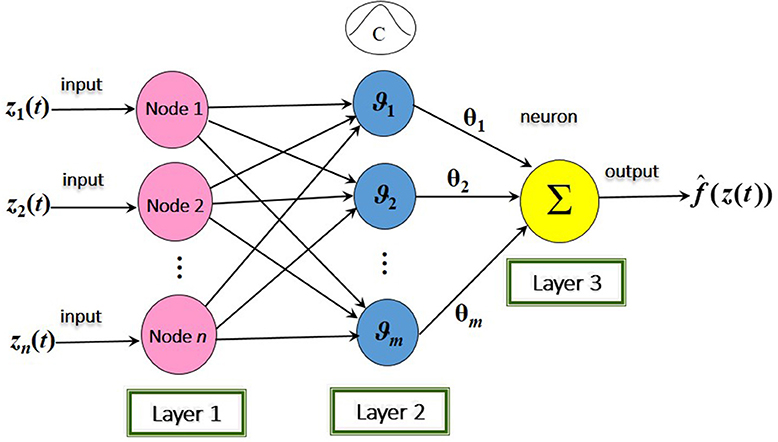
Figure 1. The structure of RBFNN.

Suppose that all of the continuous functions ϑ₁(z(t)), ϑ₂(z(t)), ⋯ , ϑ_m(z(t)) in the above RBFNN are chosen as Gaussian functions, that is, for j = 1, 2, ⋯ , m,

$\begin{array}{l}{\vartheta }_j(z(t))=exp\left(-\frac{{||z(t)-c_j||}^2}{{\sigma }_j^2}\right),\end{array}$

where $c_j={\left[c_{j1},c_{j2},\dots ,c_{jn}\right]}^T$ is the center vector and σ_j > 0 is the width of the Gaussian function ϑ_j(z(t)). Then the next lemma is obtained.

Lemma 5 ([35]). Let f :Ω → ℝ be a Lipschitz function. For each z ∈ C¹(T, Ω) and for each ε > 0, there is a RBFNN fulfilling Equation (13) and the following property:

$\begin{array}{ll}{\displaystyle \underset{t\in T}{sup}}|f(z(t))-{\theta }^T(t)\vartheta (z(t))|\le \epsilon .& (14)\end{array}$

It is well-known that non-linear theory has yet been widely applied in the stability analysis of integer-order non-linear PMSMs. Yu et al. [48] investigated a type of classical PMSMs, which are described as follows:

$\begin{array}{ll}\{\begin{array}{l}\frac{d\omega }{dt}=\sigma (i_q-\omega ),\\ \frac{d{i}_q}{dt}=-i_q-\omega i_d+\gamma \omega ,\\ \frac{d{i}_d}{dt}=-i_d+\omega i_q+u_d,\\ \end{array}& (15)\end{array}$

Yu et al. [48] also studied that when the parameters σ, γ of a PMSM decrease in a certain range, chaos will appear in the PMSM. To eliminate chaos in PMSM drive systems, they treated u_d as an adjustable variable, and proposed an adaptive NN control method based on backstepping control technique. It is well-known that backstepping technique usually makes great efforts to the effective control of integer-order triangular non-linear systems. Nevertheless, it is difficult to incorporate backstepping control technique into FONSs because of the complexities of fractional derivatives of composite functions. Moreover, the applications of FONSs broadly cover a great deal of fields, such as physics, chemistry, mathematics, etc., which suggests that the mathematical structures modeled by FONSs are more accurate and more practical.

Based on the aforementioned facts, this paper concerns a class of FOPMSMs. For simplicity, denote ω = x₁, i_q = x₂, i_d = x₃ in system (15), and extend system (15) into the next fractional-order form:

$\begin{array}{ll}\{\begin{array}{l}{{}_0{}^C{D}}_t^{\alpha }{x}_1(t)=\sigma (x_2(t)-x_1(t)),\\ {{}_0{}^C{D}}_t^{\alpha }{x}_2(t)=-x_2(t)-x_1(t)x_3(t)+\gamma x_1(t),\\ {{}_0{}^C{D}}_t^{\alpha }{x}_3(t)=-x_3(t)+x_1(t)x_2(t)+u_d(t),\end{array}& (16)\end{array}$

where 0 < α < 1, $x(t)={\left[x_1(t),x_2(t),x_3(t)\right]}^T\in {ℝ}^3$ is a measurable state-variable, x₁(t) ∈ ℝ is an output-variable, u_d(t) ∈ ℝ is an input-variable, σ and γ are positive constants, both of them represent system operating parameters.

3. Adaptive Neural Network Backstepping Control of FOPMSMs

In this section, we will improve the conventional control method combined with backstepping technique, by which the chaos of FOPMSMs realizes to be eliminated or restrained in a high effective manner. The design process includes three steps. Each of them will construct a virtual control variable based on a proper Lyapunov function. At the end, a controller in real sense will be produced to manipulate FOPMSM. Assume that x_d(t) is a given reference signal. Our goal is to establish an appropriate controller u_d(t), ensuring that the tracking error e(t): = x₁(t) − x_d(t) will ultimately converge to an arbitrarily small neighborhood of the origin. Next, we present a recursive backstepping procedure to reach our goal in three steps:

Step 1: From (16), we obtain

$\begin{array}{l}{{}_0{}^C{D}}_t^{\alpha }e(t)={{}_0{}^C{D}}_t^{\alpha }{x}_1(t)-{{}_0{}^C{D}}_t^{\alpha }{x}_d(t)\\ =\sigma (x_2(t)-x_1(t))-{{}_0{}^C{D}}_t^{\alpha }{x}_d(t)& (17)\end{array}$

The virtual control input α₁(e(t), x₁(t), x_d(t)) is adopted as

$\begin{array}{l}{\alpha }_1(e(t),x_1(t),x_d(t))=x_1(t)-\frac{1}{\sigma }[k_{11}e(t)+k_{21}\text{sign}(e(t))\\ -{{}_0{}^C{D}}_t^{\alpha }{x}_d(t)]& (18)\end{array}$

where k₁₁ > 0, k₂₁ > 0 are design parameters, sign(·) denotes a signum function.

Denote α₁(t) = α₁(e(t), x₁(t), x_d(t)). Let

$\begin{array}{ll}{e}_1(t)=x_2(t)-{\alpha }_1(t).& (19)\end{array}$

Introduce Equations (18) and (19) into Equation (17) yields

$\begin{array}{ll}{{}_0{}^C{D}}_t^{\alpha }e(t)=-k_{11}e(t)-k_{21}\text{sign}(e(t))+\sigma e_1(t).& (20)\end{array}$

Multiplying e(t) with Equation (20) generates

$\begin{array}{l}e{(t)}_0^C{{D}}_t^{\alpha }e(t)=-k_{21}\left|e(t)\right|+\sigma e(t)e_1(t)-k_{11}{e}^2(t)\\ \le \sigma e(t)e_1(t)-k_{11}{e}^2(t)& (21)\end{array}$

Let the Lyapunov function candidate V₁(t) be taken as

$\begin{array}{ll}{V}_1(t)=\frac{1}{2}{e}^2(t)& (22)\end{array}$

By Lemma 3 and Equation (21), one obtains

$\begin{array}{l}{{}_0{}^C{D}}_t^{\alpha }{V}_1(t)=\frac{1}{2}{{}_0{}^C{D}}_t^{\alpha }{e}^2(t)\le e{(t)}_0^C{{D}}_t^{\alpha }e(t)\\ \le -k_{11}{e}^2(t)+\sigma e(t)e_1(t)\\ =-{\kappa }_1{V}_1(t)+\sigma e(t)e_1(t)& (23)\end{array}$

where κ₁ = 2k₁₁ is a positive constant.

Step 2: From Equations (16) and (19), we have

$\begin{array}{l}{{}_0{}^C{D}}_t^{\alpha }{e}_1(t)={{}_0{}^C{D}}_t^{\alpha }{x}_2(t)-{{}_0{}^C{D}}_t^{\alpha }{\alpha }_1(t))\\ =-x_2(t)-x_1(t)x_3(t)+\gamma x_1(t)-{{}_0{}^C{D}}_t^{\alpha }{\alpha }_1(t)\\ =-x_2(t)-x_1(t)x_3(t)+\gamma x_1(t)-F_1(x_1(t))& (24)\end{array}$

where $F_1\left(x_1(t)\right)={{}_0{}^C{D}}_t^{\alpha }{\alpha }_1(t)$ is an unknown function. To approximate F₁(x₁(t)), we adopt a RBFNN formulated by

$\begin{array}{ll}{\widehat{F}}_1(x_1(t),{\theta }_1(t))={\theta }_1^T(t){\vartheta }_1(x_1(t)).& (25)\end{array}$

Suppose ${\theta }_1^{*}$ is the optimal parameter, which is represented as

$\begin{array}{ll}{\theta }_1^{*}=\text{arg }{\displaystyle \underset{{\theta }_1(t)}{min}}\left[{\displaystyle \underset{x_1(t)}{sup}}\left|F_1\right(x_1(t))-{\widehat{F}}_1(x_1(t),{\theta }_1(t)\left)\right|\right].& (26)\end{array}$

Here, ${\theta }_1^{*}$ is presented for the purpose of analysis, in other words, it is not required in the controller design procedure.

Define the parameter estimation error ${\tilde{\theta }}_1(t)$ as

$\begin{array}{ll}{\tilde{\theta }}_1(t)={\theta }_1(t)-{\theta }_1^{*},& (27)\end{array}$

Also, formulate the optimal approximate error ϵ₁(x₁(t)) by

$\begin{array}{ll}{ϵ}_1\left(x_1(t)\right)={\widehat{F}}_1(x_1(t),{\theta }_1^{*})-F_1\left(x_1(t)\right),& (28)\end{array}$

According to Tong and Li [49], we know that ϵ₁(x₁(t)) is bounded. Therefore,

$\begin{array}{ll}\left|{ϵ}_1\right(x_1(t)\left)\right|\le {\overline{ϵ}}_1,& (29)\end{array}$

where ${\overline{ϵ}}_1$ is a known constant. Consequently,

$\begin{array}{l}{\widehat{F}}_1(x_1(t),{\theta }_1(t))-F_1\left(x_1(t)\right)\\ ={\widehat{F}}_1(x_1(t),{\theta }_1(t))-{\widehat{F}}_1(x_1(t),{\theta }_1^{*})+{\widehat{F}}_1(x_1(t),{\theta }_1^{*})-F_1\left(x_1(t)\right)\\ ={\theta }_1^T(t){\vartheta }_1(x_1(t))-{\theta }_1^{*}{\vartheta }_1(x_1(t))+{ϵ}_1(x_1(t))\\ ={\tilde{\theta }}_1^T(t){\vartheta }_1(x_1(t))+{ϵ}_1(x_1(t)).& (30)\end{array}$

Define the virtual control input by

$\begin{array}{l}{\alpha }_2(t)=-x_1^{-1}[{\theta }_1^T(t){\vartheta }_1(x_1(t))+x_2(t)-k_{12}{e}_1(t)\\ -k_{22}\text{sign}(e_1(t))-\sigma e(t)]+\gamma & (31)\end{array}$

where k₁₂ > 0 and $k_{22}>{\overline{ϵ}}_1$ are design parameters.

Implement the following fractional-order adaptation law:

$\begin{array}{ll}{{}_0{}^C{D}}_t^{\alpha }{\theta }_1(t)=-e_1(t){\vartheta }_1(x_1(t))-{\rho }_1{\theta }_1(t),& (32)\end{array}$

where ρ₁ is a positive design parameters. Noting that the α-th order derivatives of constants are equal to 0, by Equation (27), we immediately get

$\begin{array}{ll}{{}_0{}^C{D}}_t^{\alpha }{\tilde{\theta }}_1(t)={{}_0{}^C{D}}_t^{\alpha }{\theta }_1(t).& (33)\end{array}$

Put

$\begin{array}{ll}{e}_2(t)=x_3(t)-{\alpha }_2(t).& (34)\end{array}$

Then Equations (24), (30), and (31) lead to

$\begin{array}{l}{{}_0{}^C{D}}_t^{\alpha }{e}_1(t)=-x_2(t)-x_1(t)x_3(t)+\gamma x_1(t)-F_1(x_1(t))\\ =-x_2(t)-x_1(t)x_3(t)+\gamma x_1(t)+{\tilde{\theta }}_1^T(t){\vartheta }_1(x_1(t))\\ +{ϵ}_1(x_1(t))-{\theta }_1^T(t){\vartheta }_1(x_1(t))\\ =-x_1(t)e_2(t)-k_{12}{e}_1(t)-k_{22}\text{sign}(e_1(t))-\sigma e(t)\\ +{\tilde{\theta }}_1^T(t){\vartheta }_1(x_1(t))+{ϵ}_1(x_1(t)).& (35)\end{array}$

By multiplying e₁(t) with (35), we obtain

$\begin{array}{l}{e}_1{(t)}_0^C{{D}}_t^{\alpha }{e}_1(t)=-x_1(t)e_1(t)e_2(t)-k_{12}{e}_1^2(t)\\ -k_{22}\left|e_1(t)\right|-\sigma e_1(t)e(t)\\ +e_1(t){\tilde{\theta }}_1^T(t){\vartheta }_1(x_1(t))+e_1(t){ϵ}_1(x_1(t))\\ \le -x_1(t)e_1(t)e_2(t)-k_{12}{e}_1^2(t)-\sigma e_1(t)e(t)\\ +e_1(t){\tilde{\theta }}_1^T(t){\vartheta }_1(x_1(t))+\left|e_1(t)\right|\overline{{ϵ}_1}\\ \le -x_1(t)e_1(t)e_2(t)-k_{12}{e}_1^2(t)-\sigma e_1(t)e(t)\\ +e_1(t){\tilde{\theta }}_1^T(t){\vartheta }_1(x_1(t))& (36)\end{array}$

Adopt the next Lyapunov function candidate V₂(t):

$\begin{array}{ll}{V}_2(t)=V_1(t)+\frac{1}{2}{e}_1^2(t)+\frac{1}{2}{\tilde{\theta }}_1^T(t){\tilde{\theta }}_1(t)& (37)\end{array}$

Applying Lemma 3 and Equation (23), ont gets

$\begin{array}{l}{{}_0{}^C{D}}_t^{\alpha }{V}_2(t)={{}_0{}^C{D}}_t^{\alpha }{V}_1(t)+\frac{1}{2}{{}_0{}^C{D}}_t^{\alpha }{e}_1^2(t)+\frac{1}{2}{{}_0{}^C{D}}_t^{\alpha }{\tilde{\theta }}_1^T(t){\tilde{\theta }}_1(t)\\ \le -{\kappa }_1{V}_1(t)+\sigma e_1(t)e(t)+e_1{(t)}_0^C{{D}}_t^{\alpha }{e}_1(t)\\ +{\tilde{\theta }}_1^T{(t)}_0^C{{D}}_t^{\alpha }{\tilde{\theta }}_1(t)\\ =-{\kappa }_1{V}_1(t)+\sigma e_1(t)e(t)+e_1{(t)}_0^C{{D}}_t^{\alpha }{e}_1(t)\\ +{\tilde{\theta }}_1^T{(t)}_0^C{{D}}_t^{\alpha }{\theta }_1(t)& (38)\end{array}$

Substituting Equations (36) and (32) into Equation (38) derives

$\begin{array}{l}{{}_0{}^C{D}}_t^{\alpha }{V}_2(t)\le -{\kappa }_1{V}_1(t)-x_1(t)e_1(t)e_2(t)-k_{12}{e}_1^2(t)\\ +e_1(t){\tilde{\theta }}_1^T(t){\vartheta }_1(x_1(t))+{\tilde{\theta }}_1^T{(t)}_0^C{{D}}_t^{\alpha }{\theta }_1(t)\\ =-{\kappa }_1{V}_1(t)-k_{12}{e}_1^2(t)-x_1(t)e_1(t)e_2(t)\\ -{\rho }_1{\tilde{\theta }}_1^T(t){\theta }_1(t)\\ =-{\kappa }_1{V}_1(t)-k_{12}{e}_1^2(t)-x_1(t)e_1(t)e_2(t)\\ -{\rho }_1{\tilde{\theta }}_1^T(t){\tilde{\theta }}_1(t)-{\rho }_1{\tilde{\theta }}_1^T(t){\theta }_1^{*}\\ \le -{\kappa }_1{V}_1(t)-k_{12}{e}_1^2(t)-x_1(t)e_1(t)e_2(t)\\ -\frac{{\rho }_1}{2}{\tilde{\theta }}_1^T(t){\tilde{\theta }}_1(t)+\frac{{\rho }_1}{2}{\theta }_1^{*T}(t){\theta }_1^{*}\\ \le -{\kappa }_2{V}_2(t)-x_1(t)e_1(t)e_2(t)+H_1& (39)\end{array}$

where κ₂ = min{κ₁, 2k₁₂, ρ₁} and $H_1=\frac{{\rho }_1}{2}{\theta }_1^{*T}{\theta }_1^{*}$ are positive constants.

Step 3: Using Equation (34), one has

$\begin{array}{l}{{}_0{}^C{D}}_t^{\alpha }{e}_2(t)={{}_0{}^C{D}}_t^{\alpha }{x}_3(t)-{{}_0{}^C{D}}_t^{\alpha }{\alpha }_2(t)\\ =-x_3(t)+x_1(t)x_2(t)+u_d(t)-{{}_0{}^C{D}}_t^{\alpha }{\alpha }_2(t)\\ =-x_3(t)+x_1(t)x_2(t)+u_d(t)-F_2(x_1(t),x_2(t))& (40)\end{array}$

where $F_2(x_1(t),x_2(t))={{}_0{}^C{D}}_t^{\alpha }{\alpha }_2(t)$ is unknown. We approximate F₂(x₁(t), x₂(t)) via RBFNN as follows:

$\begin{array}{ll}{\widehat{F}}_1(x_1(t),x_2(t),{\theta }_2(t))={\theta }_2^T(t){\vartheta }_2(x_1(t),x_2(t)).& (41)\end{array}$

Furthermore, Equation (40) can be reformulated by

$\begin{array}{l}{{}_0{}^C{D}}_t^{\alpha }{e}_2(t)=-x_3(t)+x_1(t)x_2(t)+u_d(t)-F_2(x_1(t),x_2(t))\\ =-x_3(t)+x_1(t)x_2(t)+u_d(t)-F_2(x_1(t),x_2(t))\\ +{\widehat{F}}_2(\underset{\_}{x_2}(t),{\theta }_2(t))-{\widehat{F}}_2(\underset{\_}{x_2}(t),{\theta }_2(t))\\ =-x_3(t)+x_1(t)x_2(t)+u_d(t)+{\tilde{\theta }}_2^T{\vartheta }_2(x_1(t),x_2(t))\\ +{ϵ}_2(x_1(t),x_2(t))-{\theta }_2^T{\vartheta }_2(x_1(t),x_2(t)).& (42)\end{array}$

Let the virtual control input be expressed by

$\begin{array}{l}{u}_d(t)=-k_{13}{e}_2(t)+x_1(t)e_1(t)-k_{23}\text{sign}(e_2(t))+x_3(t)\\ -x_1(t)x_2(t)+{\theta }_2^T{\vartheta }_2(x_1(t),x_2(t))& (43)\end{array}$

Design the fractional-order adaptation law as

$\begin{array}{ll}{{}_0{}^C{D}}_t^{\alpha }{\theta }_2(t)=-e_2(t){\vartheta }_2(x_1(t),x_2(t))-{\rho }_2{\theta }_2(t),& (44)\end{array}$

where k₁₃ > 0, $k_{23}>{\overline{ϵ}}_2$ (${\overline{ϵ}}_2$ are design parameters with $\left|\right|{ϵ}_2(x_1(t),x_2(t))\left|\right|\le {\overline{ϵ}}_2$), ρ₂ > 0. Substitute it into Equation (43). By multiplying e₂(t) with Equation (42), we get

$\begin{array}{l}{e}_2{(t)}_0^C{{D}}_t^{\alpha }{e}_2(t)=-k_{13}{e}_2^2(t)+x_1(t)e_1(t)e_2(t)-k_{23}\left|e_2(t)\right|\\ +e_2(t){\tilde{\theta }}_2^T{\vartheta }_2(x_1(t),x_2(t))+e_2(t){ϵ}_2(x_1(t),x_2(t)).& (45)\end{array}$

Choose the Lyapunov function V₃(t) as

$\begin{array}{ll}{V}_3(t)=\frac{1}{2}{e}_2^2(t)+\frac{1}{2}{\tilde{\theta }}_2^T(t){\tilde{\theta }}_2(t)+V_2(t)& (46)\end{array}$

Employing Lemma 3 with Equations (39), (44), and (45) together gives

$\begin{array}{l}{{}_0{}^C{D}}_t^{\alpha }{V}_3(t)={{}_0{}^C{D}}_t^{\alpha }{V}_2(t)+\frac{1}{2}{{}_0{}^C{D}}_t^{\alpha }{e}_2^2(t)+\frac{1}{2}{{}_0{}^C{D}}_t^{\alpha }{\tilde{\theta }}_2^T(t){\tilde{\theta }}_2(t)\\ \le -{\kappa }_2{V}_2(t)-x_1(t)e_1(t)e_2(t)+H_1+e_2{(t)}_0^C{{D}}_t^{\alpha }{e}_2(t)\\ +{\tilde{\theta }}_2^T{(t)}_0^C{{D}}_t^{\alpha }{\tilde{\theta }}_2(t))\\ \le -{\kappa }_2{V}_2(t)+H_1-k_{13}{e}_2^2(t)-{\rho }_2{\tilde{\theta }}_2^T(t){\theta }_2(t)\\ =-{\kappa }_2{V}_2(t)+H_1-k_{13}{e}_2^2(t)-{\rho }_2{\tilde{\theta }}_1^T(t){\tilde{\theta }}_1(t)\\ -{\rho }_2{\tilde{\theta }}_1^T(t){\theta }_1^{*}\\ \le -{\kappa }_2{V}_2(t)+H_1-k_{13}{e}_2^2(t)-\frac{{\rho }_2}{2}{\tilde{\theta }}_2^T(t){\tilde{\theta }}_2(t)\\ +\frac{{\rho }_2}{2}{\theta }_2^{*T}{\theta }_2^{*}\\ \le -{\kappa }_3{V}_3(t)+H_2& (47)\end{array}$

where κ₃ = min{κ₂, 2k₁₃, ρ₂} and $H_2=H_1+\frac{1}{2}{\rho }_1{\theta }_2^{*T}{\theta }_2^{*}$ are positive constants.

Theorem 1. In system (16), if the control outputs are formulated by Equations (18), (31), and (43), and the adaptation law is designed as Equations (32) and (44), then the tracking error e(t) must tend to a sufficiently small neighborhood of the equilibrium point.

Proof. Applying (47), one gets

$\begin{array}{ll}{{}_0{}^C{D}}_t^{\alpha }{V}_3(t)+\bar{Q}(t)=-{\kappa }_3{V}_3(t)+H_2& (48)\end{array}$

where $\bar{Q}(t)\ge 0$. By the implementation of the Laplace transform on Equation (48), we obtain

$\begin{array}{l}{V}_3(s)=\frac{s^{\alpha -1}}{s^{\alpha }+{\kappa }_3}{V}_3(0)+\frac{H_2}{s(s^{\alpha }+{\kappa }_3)}-\frac{M(s)}{s^{\alpha }+{\kappa }_3}\\ =\frac{s^{\alpha -1}}{s^{\alpha }+{\kappa }_3}{V}_3(0)+\frac{s^{\alpha -(1+\alpha )}{H}_2}{s^{\alpha }+{\kappa }_3}-\frac{M(s)}{s^{\alpha }+{\kappa }_3}& (49)\end{array}$

where V₃(s) and M(s) are given by the Laplace transform on V₃(t) and $\bar{Q}(t)$, respectively.

By Equations (4), (49), V₃(t) can be rearranged as

$\begin{array}{l}{V}_3(t)=V_3(0)E_{\alpha ,1}(-{\kappa }_3{t}^{\alpha })+H_2{t}^{\alpha }{E}_{\alpha ,1+\alpha }(-{\kappa }_3{t}^{\alpha })\\ -\bar{Q}(t)*t^{-1}{E}_{\alpha ,0}(-{\kappa }_3{t}^{\alpha })& (50)\end{array}$

where * denotes the convolution between functions. Since $\bar{Q}(t)$ and $t^{-1}{E}_{\alpha ,0}(-{\kappa }_3{t}^{\alpha })$ are non-negative,

$\begin{array}{l}\bar{Q}(t)*t^{-1}{E}_{\alpha ,0}(-{\kappa }_3{t}^{\alpha })\ge 0.\end{array}$

Additionally, we have

$\begin{array}{ll}\left|V_3(t)\right|\le \left|V_3(0)\right|E_{\alpha ,1}(-{\kappa }_3{t}^{\alpha })+H_2{t}^{\alpha }{E}_{\alpha ,1+\alpha }(-{\kappa }_3{t}^{\alpha }).& (51)\end{array}$

Note that $arg(-{\kappa }_3{t}^{\alpha })=-\pi$, $|-{\kappa }_3{t}^{\alpha }|\ge 0$ for any t ≥ 0 and α ∈ (0, 2). Employing Lemma 2, we deduce that there is a positive constant C with

$\begin{array}{ll}\left|E_{\alpha ,1}(-{\kappa }_3{t}^{\alpha })\right|\le \frac{C}{1+{\kappa }_3{t}^{\alpha }}.& (52)\end{array}$

It follows from Equation (52) that

$\begin{array}{ll}{\displaystyle \underset{t\to \infty }{lim}}\left|V_3(0)\right|E_{\alpha ,1}(-{\kappa }_3{t}^{\alpha })=0.& (53)\end{array}$

Therefore, for an arbitrary positive constant ε, there exists a positive constant t₁ fulfilling that

$\begin{array}{ll}\left|V_3(0)\right|E_{\alpha ,1}(-{\kappa }_3{t}^{\alpha })<\frac{\epsilon }{3},\forall t>t_1.& (54)\end{array}$

On the other hand, by employing Lemma 1, we get

$\begin{array}{ll}{E}_{\alpha ,\alpha +1}(-{\kappa }_n{t}^{\alpha })=\frac{1}{\Gamma (1){\kappa }_n{t}^{\alpha }}+o\left(\frac{1}{|{\kappa }_n{t}^{\alpha }{|}^{1+1}}\right).& (55)\end{array}$

From Equation (55), for an arbitrary ε > 0, there is a positive constant t₂ with

$\begin{array}{ll}{H}_2{t}^{\alpha }{E}_{\alpha ,\alpha +1}(-{\kappa }_3{t}^{\alpha })\le \frac{H_2}{{\kappa }_3}+\frac{\epsilon }{3},\forall t>t_2.& (56)\end{array}$

Note that the design parameter can be adjusted with $\frac{H_2}{{\kappa }_3}\le \frac{\epsilon }{3}$. Thus, coupling of Equations (51), (54), and (56) yields

$\begin{array}{ll}\left|V_3(t)\right|<\epsilon .& (57)\end{array}$

In view of Equation (57) and the definition of V₃(t), we conclude that all signals and estimation errors are bounded in the closed-loop system. Further, the tracking signal e(t) will ultimately tend toward a sufficiently small neighborhood of the equilibrium point with radius $\epsilon \ge \frac{1}{2}{e}^2(t)$ for every t > min{t₁, t₂}.□

Remark 1. Theorem 1 can be extended to the stability analysis of many other FONSs. Employing fractional-order Lyapunov stability criterion. we know that if there are two positive constants ϕ₁, ϕ₂ such that ${{}_0{}^C{D}}_t^{\alpha }V(t)\le -{\varphi }_{1}V(t)+{\varphi }_2$, where $V(t)=\frac{1}{2}{y}^T(t)y(t)$ is a Lyapunov function, then y(t) ∈ ℝⁿ is globally bounded and $y(t)\le \frac{{\varphi }_2}{{\varphi }_1}$ holds whenever the time variable t is sufficiently large.

Remark 2. In practice, the system parameters σ and γ for the model of FOPMSM are uncertain in general. Thereby, we can take advantage of the RBFNNs and adopt the corresponding adaptation law to estimate the unknown system parameters, analogizing to our proposed estimation formula (25). For the sake of simplicity, we assume that the system parameters are constants.

Remark 3. In the proposed adaptive NN backstepping control scheme, the designed controller determined by Equations (20), (31), and (43) is apparently simpler than the ones without using NN backstepping technique. Meanwhile, it is able to avert superfluous terms aroused by repeated derivation on virtual control inputs. This is beneficial especially for FONSs, in which there are a larger amount of complicated terms of fractional derivatives. For the detail, the readers may refer to Appendix B of the literature [48].

4. Numerical Simulation Example

Let us consider the next non-linear FOPMSM by setting σ = 5.6, γ = 230 and x_i(t) = y_i(t) (i = 1, 2, 3) in system (16):

$\begin{array}{ll}\{\begin{array}{l}{{}_0{}^C{D}}_t^{\alpha }{y}_1(t)=5.6(y_2(t)-y_1(t)),\\ {{}_0{}^C{D}}_t^{\alpha }{y}_2(t)=-y_2(t)-y_1(t)y_3(t)+230y_1(t),\\ {{}_0{}^C{D}}_t^{\alpha }{y}_3(t)=-y_3(t)+y_1(t)y_2(t)+u_d(t).\end{array}& (58)\end{array}$

system is proceeded under the initial condition y₀ = (−2, −0.8, 0.6). Given a reference signal y_d(t) = sin t. The chosen parameters k_1i (i = 1, 2, 3) should be >0. However, if k_1i are too large, the control gain will increase, which will consume more control energy. Therefore, in the simulation, the selected parameters k_1i are very small such that the synchronization control performs perfectly. This also shows the effectiveness of our control algorithm from another viewpoint. The adaptive parameters change much faster when the parameters are selected much larger. Based on the above considerations, The control parameters are selected as k₁₁ = k₁₂ = 1, k₁₃ = 3, ρ₁ = ρ₂ = 0.5, then we have κ₁ = κ₂ = κ₃ = 0.5.

In the aforementioned settings, there are two RBFNNs:

The first one, endowed with the input y₁(t), relies on the Gaussian radial basis functions expressed by

$\begin{array}{l}{\vartheta }_1(y_1(t))=exp\left[-\frac{1}{2}{(y_1(t)+5)}^2\right],{\vartheta }_2(y_1(t))=exp\left[-\frac{1}{2}{(y_1(t)+3)}^2\right],\\ {\vartheta }_3(y_1(t))=exp\left[-\frac{1}{2}{(y_1(t)+1)}^2\right],{\vartheta }_4(y_1(t))=exp\left[-\frac{1}{2}{(y_1(t)-1)}^2\right],\\ {\vartheta }_5(y_1(t))=exp\left[-\frac{1}{2}{(y_1(t)-3)}^2\right],{\vartheta }_6(y_1(t))=exp\left[-\frac{1}{2}{(y_1(t)-5)}^2\right],\end{array}$

respectively. The radial basis functions are shown in Figure 2. The initial condition is taken as ${\theta }_1(0)={\left[1,1,1,1,1,1\right]}^T\in {ℝ}^6$, uniformly distributed on [−5, 5].

FIGURE 2

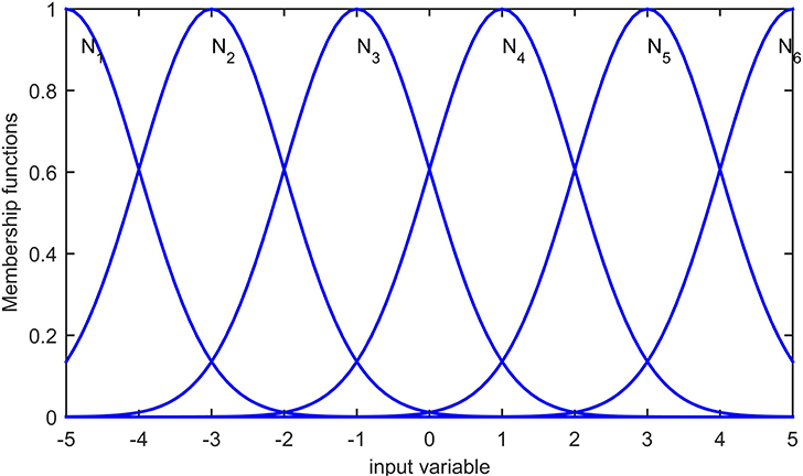
Figure 2. The radial basis functions for RBFNN.

Another RBFNN utilizes y₁(t) and y₂(t) as its inputs. Choose the Gaussian radial basis functions to be the same as that of the previous RBFNN for every input. The initial condition is fixed as ${\theta }_2(0)={\left[1,1,\cdots ,1\right]}^T\in {ℝ}^{36}$.

On the basis of the above settings, the drive system of FOPMSM is simulated as follows:

Firstly, when α = 0.98 and u_d(t) = 0, the chaotic phenomenon of the FOPMSM drive system is tested, demonstrating that system (58) is not stable, as illustrated in Figure 3.

FIGURE 3

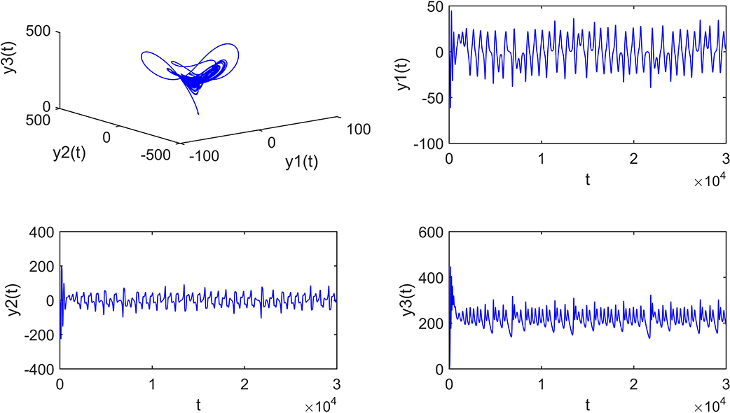
Figure 3. Dynamic behavior of FOPMSM.

Secondarily, we apply the proposed adaptive RBFNN backstepping method in the control procedure of chaotic FOPMSM, which is depicted in Figure 4.

FIGURE 4

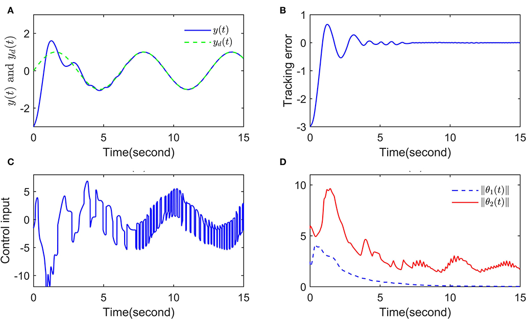
Figure 4. The simulation diagrams, (A) The signals y(t) and y_d(t), (B) The tracking error, (C) The control input, (D) The parameter norms of RBFNN.

Finally, as a summary, it is evident that the proposed controller makes an effective effort to restrain the chaos of FOPMSM drive system, and it embodies desirable performance during the signal tracking.

5. Conclusion

This work provides a framework to study stabilization control of chaotic FOPMSMs on the basis of extended Lyapunov stability criterion. Our results as well as numerical simulations indicate that when the proposed adaptive NN backstepping-based control scheme is employed to control chaotic FOPMSMs, it indeed facilitates to overcome the inherent drawback “explosion of complexity.” It is demonstrated that chaos and oscillation may appear apparently in the system when the system is uncontrolled. Through the control proceeding, the variables become regular, the chaos oscillation is suppressed, and the task of signal tracking is perfectly accomplished. The problem about how to further construct an adaptive NN backstepping control scheme for generalized FOPMSMs with more input uncertainties and non-linearities is open, which is one task of our future works.

Data Availability Statement

All datasets generated for this study are included in the article/supplementary material.

Author Contributions

GX, FL, and BQ contributed the conception and design of the study. GX organized the literature. FL performed the design of figures. GX wrote the first draft of the manuscript. All authors contributed to the manuscript revision, read, and approved the submitted version.

Funding

This work was supported the Basic Ability Promotion Project for Young and Middle-aged Teachers of Guangxi Colleges and Universities (Grant No. 2019KY0669), the Scientific Research Development Fund of Young Researchers of Guangxi University of Finance and Economics (Grant No. 2019QNB18).

Conflict of Interest

The authors declare that the research was conducted in the absence of any commercial or financial relationships that could be construed as a potential conflict of interest.

Acknowledgments

The authors would like to express their sincere gratitude to the reviewers and the editors for their careful reviews and constructive recommendations.

Footnote

1. ^A function ĝ :[0, ∞) → T is said to belong to class-K if it is strictly increasing, continuous and ĝ(0) = 0.

References

1. Podlubny I. Fractional Differential Equations. San Diego, CA: Academic Press (1999).

Google Scholar

2. Bagley RL, Torvik PJ. Fractional calculus–a different approach to the analysis of viscoelastically damped structures. AIAA J. (1983) 21:741–8. doi: 10.2514/3.8142

CrossRef Full Text | Google Scholar

3. Chen W, Ye L, Sun H. Fractional diffusion equations by the Kansa method. Comput Math Appl. (2010) 59:1614–20. doi: 10.1016/j.camwa.2009.08.004

CrossRef Full Text | Google Scholar

4. Radwan AG, Elwakil AS, Soliman AM. Fractional-order sinusoidal oscillators: design procedure and practical examples. IEEE Trans Circuits Syst I Reg Pap. (2008) 55:2051–63. doi: 10.1109/TCSI.2008.918196

CrossRef Full Text | Google Scholar

5. Wang J, Ibrahim AG, Fečkan M. Nonlocal impulsive fractional differential inclusions with fractional sectorial operators on Banach spaces. Appl Math Comput. (2015) 257:103–18. doi: 10.1016/j.amc.2014.04.093

CrossRef Full Text | Google Scholar

6. Podlubny I. Geometric and physical interpretation of fractional integration and fractional differentiation. Fract Calculus Appl Anal. (2002) 5:367–86. doi: 10.1016/j.sigpro.2014.05.026

CrossRef Full Text | Google Scholar

7. Baleanu D, Golmankhaneh AK, Golmankhaneh AK. On electromagnetic field in fractional space. Nonlin Anal Real World Appl. (2010) 11:288–92. doi: 10.1016/j.nonrwa.2008.10.058

CrossRef Full Text | Google Scholar

8. Kilbas AAA, Srivastava HM, Trujillo JJ. Theory and Applications of Fractional Differential Equations. Vol. 204. Amsterdam: Elsevier Science Limited (2006).

Google Scholar

9. Tsirimokou G, Psychalinos C, Elwakil AS. Fractional-order electronically controlled generalized filters. Int J Circuit Theory Appl. (2017) 45:595–612. doi: 10.1002/cta.2250

CrossRef Full Text | Google Scholar

10. Tsirimokou G, Psychalinos C, Elwakil A. Design of CMOS Analog Integrated Fractional-Order Circuits: Applications in Medicine and Biology. Cham: Springer (2017).

Google Scholar

11. Zhou Y, Liu H, Cao J, Li S. Composite learning fuzzy synchronization for incommensurate fractional-order chaotic systems with time-varying delays. Int J Adapt Control. (2019) 33:1739–58. doi: 10.1002/acs.2967

CrossRef Full Text | Google Scholar

12. Wang LX. Adaptive Fuzzy Systems and Control: Design and Stability Analysis. Englewood Cliffs, NJ: Prentice-Hall, Inc. (1994).

Google Scholar

13. Radwan AG, Soliman A, Elwakil AS, Sedeek A. On the stability of linear systems with fractional-order elements. Chaos Solit Fract. (2009) 40:2317–28. doi: 10.1016/j.chaos.2007.10.033

CrossRef Full Text | Google Scholar

14. You X, Song Q, Zhao Z. Global Mittag-Leffler stability and synchronization of discrete-time fractional-order complex-valued neural networks with time delay. Neural Netw. (2020) 122:382–94. doi: 10.1016/j.neunet.2019.11.004

PubMed Abstract | CrossRef Full Text | Google Scholar

15. You X, Song Q, Zhao Z. Existence and finite-time stability of discrete fractional-order complex-valued neural networks with time delays. Neural Netw. (2020) 123:248–60. doi: 10.1016/j.neunet.2019.12.012

PubMed Abstract | CrossRef Full Text | Google Scholar

16. Liu H, Pan Y, Cao J, Zhou Y, Wang H. Positivity and stability analysis for fractional-order delayed systems: a T-S fuzzy model approach. IEEE Trans Fuzzy Syst. (2020). doi: 10.1109/TFUZZ.2020.2966420. [Epub ahead of print].

CrossRef Full Text | Google Scholar

17. Kurths J, Boccaletti S, Grebogi C, Lai YC. Introduction: control and synchronization in chaotic dynamical systems. Chaos. (2003) 13:126–7. doi: 10.1063/1.1554606

PubMed Abstract | CrossRef Full Text | Google Scholar

18. Radwan AG, Moaddy K, Salama KN, Momani S, Hashim I. Control and switching synchronization of fractional order chaotic systems using active control technique. J Adv Res. (2014) 5:125–32. doi: 10.1016/j.jare.2013.01.003

PubMed Abstract | CrossRef Full Text | Google Scholar

19. Kuroe Y, Hayashi S. Analysis of bifurcation in power electronic induction motor drive systems. In: 20th Annual IEEE Power Electronics Specialists Conference. Milwaukee, WI: IEEE (1989). p. 923–30.

Google Scholar

20. Chen J, Chau K, Siu S, Chan C. Experimental stabilization of chaos in a voltage-mode DC drive system. IEEE Trans Circuits Syst I Fundam Theory Appl. (2000) 47:1093–5. doi: 10.1109/81.855466

CrossRef Full Text | Google Scholar

21. Robert B, Alin F, Goeldel C. Aperiodic and chaotic dynamics in hybrid step motor-new experimental results. In: ISIE 2001. 2001 IEEE International Symposium on Industrial Electronics Proceedings (Cat. No. 01TH8570). Vol. 3. Pusan: IEEE (2001). p. 2136–41.

Google Scholar

22. Gao Y, Chau K, Ye S. A novel chaotic-speed single-phase induction motor drive for cooling fans. In: Fourtieth IAS Annual Meeting. Conference Record of the 2005 Industry Applications Conference, 2005. Vol. 2. IEEE (2005). p. 1337–41.

Google Scholar

23. Wei D, Luo X. Passive adaptive control of chaos in synchronous reluctance motor. Chin Phys B. (2008) 17:92–7. doi: 10.1088/1674-1056/17/1/017

CrossRef Full Text | Google Scholar

24. Chau K, Chen J. Modeling, analysis, and experimentation of chaos in a switched reluctance drive system. IEEE Trans Circuits Syst I Fundam Theory Appl. (2003) 50:712–6. doi: 10.1109/TCSI.2003.811030

CrossRef Full Text | Google Scholar

25. Ott E, Grebogi C, Yorke JA. Controlling chaos. Phys Rev Lett. (1990) 64:1196. doi: 10.1103/PhysRevLett.64.1196

PubMed Abstract | CrossRef Full Text | Google Scholar

26. Ren H, Liu D. Nonlinear feedback control of chaos in permanent magnet synchronous motor. IEEE Trans Circuits Syst II Express Briefs. (2006) 53:45–50. doi: 10.1109/TCSII.2005.854592

CrossRef Full Text | Google Scholar

27. Pan Y, Sun T, Yu H. On parameter convergence in least squares identification and adaptive control. Int J Robust Nonlin. (2019) 29:2898–911. doi: 10.1002/rnc.4527

CrossRef Full Text | Google Scholar

28. Liu H, Wang H, Cao J, Alsaedi A, Hayat T. Composite learning adaptive sliding mode control of fractional-order nonlinear systems with actuator faults. J Franklin Inst. (2019) 356:9580–99. doi: 10.1016/j.jfranklin.2019.02.042

CrossRef Full Text | Google Scholar

29. Luo XS, Wang BH, Fang JQ, Wei DQ. Robust adaptive dynamic surface control of chaos in permanent magnet synchronous motor. Phys Lett A. (2007) 363:71–7. doi: 10.1016/j.physleta.2006.10.074

CrossRef Full Text | Google Scholar

30. Balasubramaniam P, Muthukumar P, Ratnavelu K. Theoretical and practical applications of fuzzy fractional integral sliding mode control for fractional-order dynamical system. Nonlin Dyn. (2015) 80:249–67. doi: 10.1007/s11071-014-1865-4

CrossRef Full Text | Google Scholar

31. Li H, Wang J, Wu L, Lam HK, Gao Y. Optimal guaranteed cost sliding-mode control of interval type-2 fuzzy time-delay systems. IEEE Trans Fuzzy Syst. (2018) 26:246–57. doi: 10.1109/TFUZZ.2017.2648855

CrossRef Full Text | Google Scholar

32. Harb AM. Nonlinear chaos control in a permanent magnet reluctance machine. Chaos Solit Fract. (2004) 19:1217–24. doi: 10.1016/S0960-0779(03)00311-4

CrossRef Full Text | Google Scholar

33. Stotsky A, Hedrick J, Yip P. The use of sliding modes to simplify the backstepping control method. In: Proceedings of the 1997 American Control Conference (Cat. No. 97CH36041). Vol. 3. Albuquerque, NM: IEEE (1997). p. 1703–8. doi: 10.1109/ACC.1997.610875

CrossRef Full Text | Google Scholar

34. Liu H, Pan Y, Li S, Chen Y. Adaptive fuzzy backstepping control of fractional-order nonlinear systems. IEEE Trans Syst Man Cybern Syst. (2017) 47:2209–17. doi: 10.1109/TSMC.2016.2640950

CrossRef Full Text | Google Scholar

35. Liu H, Pan Y, Jinde C, Hongxing W, Yan Z. Adaptive neural network backstepping control of fractionial-order nonlinear systems with actuator faults. IEEE Trans Neural Netw Learn Syst. (2020). doi: 10.1109/TNNLS.2020.2964044. [Epub ahead of print].

PubMed Abstract | CrossRef Full Text | Google Scholar

36. Gao H, Song Y, Wen C. Event-triggered adaptive neural network controller for uncertain nonlinear system. Inform Sci. (2020) 506:148–60. doi: 10.1016/j.ins.2019.08.015

CrossRef Full Text | Google Scholar

37. Bai W, Li T, Tong S. NN reinforcement learning adaptive control for a class of nonstrict-feedback discrete-time systems. IEEE Trans Cybern. (2020). doi: 10.1109/TCYB.2020.2963849. [Epub ahead of print].

PubMed Abstract | CrossRef Full Text | Google Scholar

38. Boulkroune A, Tadjine M, M'Saad M, Farza M. Fuzzy adaptive controller for MIMO nonlinear systems with known and unknown control direction. Fuzzy Sets Syst. (2010) 161:797–820. doi: 10.1016/j.fss.2009.04.011

CrossRef Full Text | Google Scholar

39. Boulkroune A, Bouzeriba A, Bouden T. Fuzzy generalized projective synchronization of incommensurate fractional-order chaotic systems. Neurocomputing. (2016) 173:606–14. doi: 10.1016/j.neucom.2015.08.003

CrossRef Full Text | Google Scholar

40. Shukla MK, Sharma BB. Backstepping based stabilization and synchronization of a class of fractional order chaotic systems. Chaos Solit Fract. (2017) 102:274–84. doi: 10.1016/j.chaos.2017.05.015

CrossRef Full Text | Google Scholar

41. Zhou J, Wen C, Wang W, Yang F. Adaptive backstepping control of nonlinear uncertain systems with quantized states. IEEE Trans Autom Control. (2019) 64:4756–63. doi: 10.1109/TAC.2019.2906931

CrossRef Full Text | Google Scholar

42. Yip PP, Hedrick JK. Adaptive dynamic surface control: a simplified algorithm for adaptive backstepping control of nonlinear systems. Int J Control. (1998) 71:959–79. doi: 10.1080/002071798221650

CrossRef Full Text | Google Scholar

43. Kwan C, Lewis FL. Robust backstepping control of induction motors using neural networks. IEEE Trans Neural Netw. (2000) 11:1178–87. doi: 10.1109/72.870049

PubMed Abstract | CrossRef Full Text | Google Scholar

44. Dawson DM, Carroll JJ, Schneider M. Integrator backstepping control of a brush DC motor turning a robotic load. IEEE Trans Control Syst Technol. (1994) 2:233–44. doi: 10.1109/87.317980

CrossRef Full Text | Google Scholar

45. Fateh S, Fateh MM. Adaptive fuzzy control of robot manipulators with asymptotic tracking performance. J Control Autom Electric Syst. (2020) 31:52–61. doi: 10.1007/s40313-019-00496-5

CrossRef Full Text | Google Scholar

46. Li Y, Chen Y, Podlubny I. Mittag-Leffler stability of fractional order nonlinear dynamic systems. Automatica. (2009) 45:1965–9. doi: 10.1016/j.automatica.2009.04.003

CrossRef Full Text | Google Scholar

47. Li Y, Tong S. Adaptive neural networks decentralized FTC design for nonstrict-feedback nonlinear interconnected large-scale systems against actuator faults. IEEE Trans Neural Netw Learn Syst. (2016) 28:2541–54. doi: 10.1109/TNNLS.2016.2598580

PubMed Abstract | CrossRef Full Text | Google Scholar

48. Yu J, Chen B, Yu H, Gao J. Adaptive fuzzy tracking control for the chaotic permanent magnet synchronous motor drive system via backstepping. Nonlin Anal Real World Appl. (2011) 12:671–81. doi: 10.1016/j.nonrwa.2010.07.009

CrossRef Full Text | Google Scholar

49. Tong S, Li Y. Adaptive fuzzy output feedback control of MIMO nonlinear systems with unknown dead-zone inputs. IEEE Trans Fuzzy Syst. (2012) 21:134–46. doi: 10.1109/TFUZZ.2012.2204065

CrossRef Full Text | Google Scholar