Onsager-Symmetry Obeyed in Athermal Mesoscopic Systems: Two-Phase Flow in Porous Media

We compute the fluid flow time correlation functions of incompressible, immiscible two-phase flow in porous media using a 2D network model. Given a properly chosen representative elementary volume, the flow rate distributions are Gaussian, and the integrals of time correlation functions of the flows are found to converge to a finite value. The integrated cross-correlations become symmetric, obeying Onsager's reciprocal relations. These findings support the proposal of a non-equilibrium thermodynamic description for two-phase flow in porous media.

1. Introduction

Athermal fluctuations occur in a number of phenomena in nature and are important to biology, chemistry, and physics [1–3]. Currently, an active effort is being made to better understand the statistical physics of such systems, and its use is realized in a growing number of research areas [1, 3–8]. A particular example is granular materials, the constituents of which are macroscopic. In the absence of an external driving force, the material will stay in its current configuration, sharing some properties with non-ergodic systems [3]. However, when a granular material is exposed to an external force, a great number of states may be visited, resulting in solid- or fluid-like behavior as a response to that force.

One area that seems not to have been analyzed in these terms is flow driven through porous media. Such flows are important for numerous geological and technical processes, for example, in oil production, CO₂ sequestration, water transport in aquifers, or heterogeneous catalysis. An important class of porous media flows is the simultaneous flow of two immiscible fluids. In such a system, clusters of the two fluid phases, traveling through the porous medium, are constantly forced to split and recombine. Thus, the fluid configuration in the pore space changes, leading to fluctuations in the flow rate of each phase (fractional flow rate), as well as in the total flow rate. These fluctuations are of a mechanical nature and are different from but analogous to thermal fluctuations on the molecular level. The fluctuations appear on a mesoscopic scale much larger than the molecular scale of statistical thermodynamics, yet the mesoscopic scale that is defined by the pore sizes of the medium is very small compared to the overall system. In the most extreme cases, the pores can be in the nanosize regime, while the system of interest, for instance, in chalk oil reservoirs [9], has geological dimensions.

Our long-term aim is to find a non-equilibrium thermodynamic description for such flow systems. The challenge is then to define a suitable representative elementary volume (REV) where the essential assumption of local equilibrium, as expressed by the ergodic hypothesis, and microscopic reversibility hold. The statistical foundation of the theory was spelled out a long time ago [10]. Experimental [11] and computational [12, 13] evidence now exist that the ergodic hypothesis can be expected to hold for immiscible two-phase flow in two-dimensional porous media of a minimum number of links.

Here, the aim is to move one step forward and examine the idea of time-reversal invariance or the microscopic reversibility of fluctuations [10, 14]. Thus, our interest is in the time correlation functions of the flows. On the molecular scale, thermal fluctuations have correlation functions that are connected to transport coefficients. This is formulated in the Green–Kubo relations, which are frequently employed in molecular dynamic simulations. The method goes back to Onsager's regression hypothesis [15, 16], which says that the decay of molecular fluctuations is governed by the same laws as the relaxation of macroscopic non-equilibrium disturbances. For the Onsager reciprocal relations [15, 16] to apply, microscopic reversibility must hold. The idea of the present work is to apply Green–Kubo-like relations to the fluctuations in an REV of a network model. The Green–Kubo relations for the molecular level apply to global equilibrium. In the present approach, we will use similar expressions but for fluctuations on the mesoscale, thereby extending or expanding the Green–Kubo-scheme. We shall see that the system models a time reversal-invariant process and that the integrated flux correlations satisfy Onsager symmetry. A similar approach to fluctuations in hydrodynamic dispersion was taken by Flekkøy et al. [17].

In the present study, we use a dynamic pore network model to simulate immiscible two-phase flow in porous media. This model, introduced in the late nineties [18], was developed for and calibrated against the bead-filled Hele-Shaw cell used for experimentally studying such flow. For example, the pressure fluctuations in the dynamic network model were shown to match very well with those observed in the experimental system [19]. A recent comparison between model and experiment may be found in Zhao et al. [20]. In the present implementation of the model, we use a network based on a hexagonal lattice, where the links represent pore throats and have a spatially uncorrelated distribution of link radii. The steady flow of two incompressible and immiscible fluids is driven by a constant pressure difference across the network, leading to a steady state with fluctuating fluid flow. The flow properties fluctuate around well-defined values, and the system is in a non-equilibrium steady state on the network level of description. A correlation of the two flows is thus unavoidable. But what is the nature of this correlation? The answer will have an impact on how we may proceed with a theoretical description of the flows.

A crucial question that needs to be answered is whether the dynamic network model is ergodic or not. Flekkøy and Pride [21] argue that immiscible two-phase flow at the pore scale is only ergodic if the interfaces do not move or move very little. However, at the molecular scale, there is ergodicity. Hence, ergodicity may be lost through the way the system is described. When the pores are assembled into a porous medium so that the motion of the fluids is a collective phenomenon, Savani et al. argue and demonstrate, based on the dynamic pore network model, that ergodicity is restored [12, 13]. This was done by rewriting time averages for the dynamic network model as configurational averages and thereby constructing the ensemble probability function explicitly.

If one considers a steady state of immiscible two-phase flow, as we will in our model, we shall see that the fluctuations become Gaussian around a steady mean.

Hence, the concept of the REV at steady state is highly relevant and important for how we build a theory that can help us understand transport in porous media.

2. Model

The transport of the two immiscible fluids through a two-dimensional porous medium is represented by a dynamical pore network model [18, 22]. This model has been in development for over two decades and has a record of explaining experimental and theoretical results in steady and transient two-phase flow in porous media [11–13, 18, 20, 22–25]. In this model, the two fluids are separated by interfaces and are flowing in a network of links that are connected at nodes. The network has a honeycomb structure, as illustrated in Figure 1, with equally long links and a distribution of link radii. The radii are drawn from a uniform distribution in the interval 0.1 to 0.4 L, where L is the length of the links. The flow rate q_ij inside a link connecting nodes j and i is given by:

$\begin{array}{ll}{q}_{ij}=-g_{ij}[p_j-p_i-c_{ij}(z_{ij})].& (1)\end{array}$

FIGURE 1

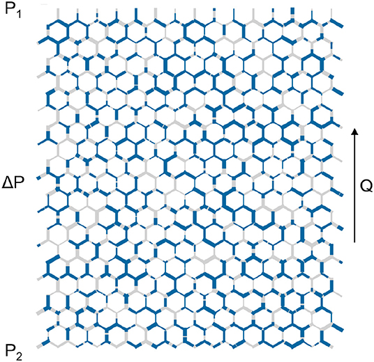
Figure 1. Illustration of the network model. The network is occupied by two immiscible fluids (blue and gray colors). The equally long links (pores) have an hourglass-shaped structure and a random distribution of diameters.

Here, p_j and p_i are the pressures at nodes j and i, c_ij is the capillary pressure, and g_ij is the conductivity of the link. The links have an hourglass shape, and thus the capillary pressure is a function of the interface positions, z_ij:

$\begin{array}{ll}{c}_{ij}(z_{ij})=\frac{2\gamma }{r_{ij}}{\displaystyle \sum _{z\in z_{ij}}(\pm 1)}\left\{1-\cos (2\pi \chi (z))\right\}.& (2)\end{array}$

Here, γ is the surface tension, r_ij is the radius of link ij, and

$\begin{array}{ll}\chi (z)=\{\begin{array}{ll}0,\hfill & \text{if }z<\beta r_{ij},\hfill \\ \frac{z-\beta r_{ij}}{L-2\beta r_{ij}},\hfill & \text{if }\beta r_{ij}<z<L-\beta r_{ij},\hfill \\ 1,\hfill & \text{if }z>L-\beta r_{ij}.\hfill \end{array}& (3)\end{array}$

The effect of the χ-function is to introduce zones of length βr_ij at each end of the links where the pressure discontinuity of any interface is zero. The conductivity of the link, g_ij, contains a geometrical factor and the effective viscosity of the link:

$\begin{array}{ll}{g}_{ij}=\frac{\pi r_{ij}^4}{8L\mu (S_{w,ij})}.& (4)\end{array}$

Here, r_ij is the radius of the link, and the viscosity is defined as

$\begin{array}{ll}\mu (S_{w,ij})=S_{w,ij}{\mu }_w+(1-S_{w,ij}){\mu }_n,& (5)\end{array}$

with S_{w, ij} being the saturation (i.e., the volume fraction) of the wetting phase in link ij. Simulations were carried out, applying a constant global pressure drop ΔP across the network. Periodic boundary conditions are used in all directions. The local pressures p_i are determined by solving the Kirchhoff equations. Further details of the model and solution methods can be found in Sinha et al. [22] and Gjennestad et al. [24]. For each link, the flow rate q_ij is calculated using Equation (1), and the positions of the interfaces are advanced with an appropriately small, constant time step of 10⁻⁵ s. A constant time step is used to facilitate a convenient calculation of the time-correlation functions. The simulations were started with a random distribution of the two liquid phases and were propagated at least 300,000 time steps to allow the system to reach a steady state. Statistics for the time correlation functions were collected for 9.7 million time steps. The length of a link in the network was set to 1 mm. We report results for each set of parameters as averages of at least 30 runs using different starting configurations of the two fluids. Volume flow rates and velocities refer to network averages. The properties of the steady-state flow are determined by the pressure drop across the system, ΔP, the total wetting saturation of the network, the surface tension, γ, and the viscosity of the two fluids. We have ensured that the same steady-state flow averages are obtained from different initial distributions of the two fluids, including an initial configuration where the two phases are completely separated (i.e., each phase is in a single connected cluster). Furthermore, it has been tested that a different link radii configuration drawn from the same uniform distribution does not change the steady flow averages nor the appearance of the time correlation functions computed in this study.

We investigated time correlation functions and their long-time convergence for two choices of the parameter set μ_w, μ_n, and γ, which are viscosities of the wetting and the non-wetting phase and the surface tension, respectively.

Case (A) had viscosities ${\mu }_w={\mu }_n=10^{-3}$ Pa·s and different choices for the pressure gradient (100–200 kPa/m) and the surface tension γ = 3–30 mN/m. At steady state, the capillary number was Ca ≈ 10⁻³ – 10⁻². Here, the capillary number is defined as Ca = vμ_n/γ, with v being the seepage velocity. The case was chosen to represent flow where the two fluids are interchangeable with respect to their viscous dissipation.

Case (B) had μ_w = 5μ_n (${\mu }_w=10^{-3}$ Pa·s) and γ = 0. This case is typical at high flow rates where the contribution from γ essentially can be neglected, and the capillary number goes to infinity. It can be considered as a limiting case, chosen to elucidate the behavior when viscous forces dominate and the surface tension is negligible. Data were collected for wetting phase saturation S_w = 0.25, 0.5, and 0.75. Here, S_w is the volume fraction of the wetting phase of the total pore volume in the network.

3. Results and Discussion

We report first that the fluctuations in flow velocities are Gaussian when a suitable representative volume (REV) is chosen. We proceed to give the structure of the time correlation functions for the REV. The results for what we will call from now the Green–Kubo coefficients for the network follow from this.

3.1. Fluctuations

In case (A), the resistance is determined by the positions of the interfaces in the links only, as the two phases have the same viscosity. In case (B), the resistance to flow in link i is inversely proportional to the effective viscosity. The positions of the interfaces are then irrelevant, as there is no surface tension and hence, no capillary pressure.

A typical example of fluctuations in the total volume flow Q for case (A), with a pressure gradient ΔP/Δx of 100 kPa/m and surface tension 30 mN/m, is shown in Figure 2. By plotting the statistical frequency of the flow rate or the seepage velocity, we obtain a Gaussian distribution. This is shown in Figure 3, where we plot the statistical frequency of the fluid velocity (counts) on a logarithmic scale vs. $sgn(v-v_0){(v-v_0)}^2$. In such a plot, a Gaussian distribution appears as a triangle, and this behavior is very well followed by the data. There is only a very small asymmetry in the distribution, which is to be expected as the fluid velocity cannot be less than zero. A regular plot of the distributions is presented for the seepage velocity and the velocities of the wetting and non-wetting phases in Figure 4. The distributions are shown for two network sizes of case (A), one with 30 × 20 links and one twice the size, with 60 × 40 links. The shown distributions are normalized to the area, and the variance of the larger network is half the width of that of the smaller network. So, in spite of the apparent noise seen in Figure 2, one obtains the distributions shown in Figure 4, which has its analog in molecular statistical thermodynamics, basic to thermodynamic equilibrium properties. This allows us to proceed with the next step and construct time correlation functions for the meso-level.

FIGURE 2

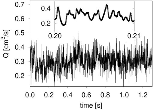
Figure 2. Fluctuations of the volumetric flow Q for case A (see text). The pressure gradient was 100 kPa/m. During the time span shown, 1.3 s, a volume twice the total volume of the network has passed. The inset shows the same quantity over a short time interval.

FIGURE 3

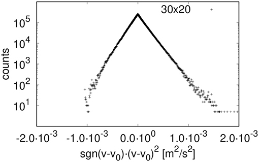
Figure 3. Distribution of network-averaged instantaneous total (wetting and non-wetting) fluid velocity for network size 30 x 20 (case A). v₀ is the total average velocity and sgn is the sign function.

FIGURE 4

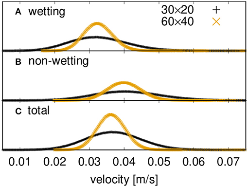
Figure 4. Distributions of network-averaged instantaneous fluid velocities for two network sizes (30 × 20, 60 × 40).

3.2. Network Size and Representative Volume

Ideally, the system size of the simulation is sufficiently large and representative of the statistical ensemble. In this, the entropy and other thermodynamic properties are proportional to the system size (i.e., they are extensive [26]). With the Gaussian nature, one may expect that the inverse variance 1/σ² of the fluctuations is proportional to the system size, i.e., the area A. This relation is plotted in Figure 5 for network models of dimension 30 × 20, 60 × 40, and 120 × 60 links. It shows that this requirement is well met by a system with low Ca, but systems with higher Ca may be more susceptible to possible size effects. The size of the REV will be system-dependent; see Savani et al. [13]. But in the present cases, (A) and (B), an REV can be defined for a range of Ca. The results for the REV comply with the meso-level analog we are seeking.

FIGURE 5

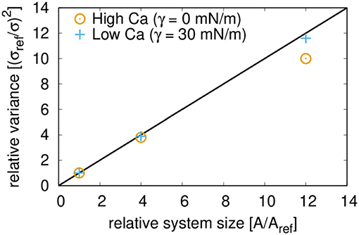
Figure 5. Scaling of the variance σ² of the flow velocity size distributions with system size.

3.3. Time Correlation Functions

With a well-defined REV, and with Gaussian fluctuations established, we can proceed to define the time correlation functions C_RS for the fluctuating quantities R and S at the meso-level:

$\begin{array}{ll}{C}_{RS}(\tau )=\langle \delta R(0)\delta S(\tau )\rangle =\langle R(0)S(\tau )\rangle -\langle R\rangle \langle S\rangle ,& (6)\end{array}$

where the brackets 〈⋯ 〉 indicate ensemble averages.

The fluctuation from the mean, δR, is defined as

$\begin{array}{ll}\delta R(t)=R(t)-\langle R\rangle ,& (7)\end{array}$

and

$\begin{array}{ll}\langle \delta R\rangle =0.& (8)\end{array}$

Figure 6 shows the time correlation functions of the total flow rate Q for different choices of the surface tension. After a rapid decay on a short timescale (below 10⁻³ s) there is a slower, logarithmic decay which is more pronounced for larger values of γ (between 1 and 100 ms). These two regimes are followed by a slow long-timescale decay. The rapid decay appears on the timescale that corresponds to the time necessary to evolve the flow by one average link volume. As shown in Figure 6, the decay is somewhat faster for smaller surface tensions as the total flow velocity is higher.

FIGURE 6

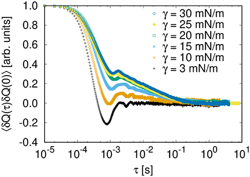
Figure 6. Dependence of (scaled) time correlation function 〈Q(τ)Q(0)〉 on the surface tension γ (case (A) with ΔP/Δx = 100 kPa/m and network size of 30 × 20 links).

The regime of the logarithmic decay is within the time of evolving the flow by the total volume of the network and is more pronounced for higher surface tensions and thus higher capillary pressures in the pores. Hence, the decay corresponds to parts of the flow that are slow-moving or frustrated. These are the regimes of interest here. They contain the relative movements of the two flows in terms of their mutual displacement.

It is interesting to note some similarities with time correlation functions of glass [27] or yield-stress fluids [28]. In these cases, the autocorrelation functions, like the self-scattering function, can be fitted to a function of the form:

$\begin{array}{ll}F(t)=aexp\left[-{(t/{\tau }_1)}^{\alpha }\right]+bexp\left[-{(t/{\tau }_2)}^{\beta }\right].& (9)\end{array}$

We attempted a fit of F(t) to the autocorrelation functions of the total flow; see Figure 7. Satisfying fits could be obtained with the exception that the local minimum and maximum at around 10⁻³ s and in some cases the flat top (at times < 10⁻⁴ s) are not well-described. Fit parameters for the different choices of γ are summarized in Table 1.

FIGURE 7

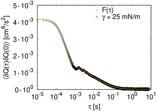
Figure 7. Fit of function F(t) (Equation 9) to the autocorrelation function of the total volume flow for case (A) with γ = 25 mN/m (ΔP/Δx = 100 kPa/m and 30 × 20 links).

TABLE 1

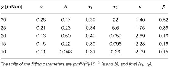
Table 1. Fitting parameters for F(t) (see Equation 9) to the autocorrelation functions of the total flow for different values of γ.

3.4. Convergence and Symmetry

The Green–Kubo method employs integrals of suitable time correlation functions C_RS (as defined in Equation 6) to compute coefficients, L_RS:

$\begin{array}{ll}{L}_{RS}={\displaystyle {\int }_0^{\infty }}{C}_{RS}(\tau )d\tau .& (10)\end{array}$

The convergence of the integral over the time correlation function of the total flow is shown in Figure 8. As in molecular dynamics, where the Green–Kubo method is normally used, the convergence is slow, and statistics have to be collected over long timescales and/or multiple trajectories to achieve convergence of the integral when τ is approaching infinity.

FIGURE 8

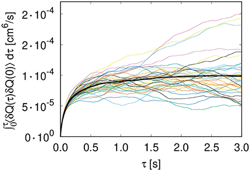
Figure 8. Convergence of the integrated time correlation function [case (A), γ = 30 mN/m and 30 × 20 links]. The colored lines represent individual trajectories; the thicker black line is the average of all trajectories.

We computed the integrals for the autocorrelation and cross-correlation functions of the wetting and non-wetting phases,

$\begin{array}{ll}{\Lambda }_{ij}={\displaystyle {\int }_0^{\infty }}[\langle Q_i(\tau )Q_j(0)\rangle -\langle Q_i\rangle \langle Q_j\rangle ]d\tau ,& (11)\end{array}$

with the indexes i, j = n, w referring to the non-wetting and wetting phase, respectively. The results are listed in Table 2 for case (A), where the surface tension is 30 mN/m and the fluids have the same viscosity, for three different choices of ΔP, the pressure difference across the network. Table 3 lists the corresponding flow properties for case (A). Table 4 summarizes results for infinite capillary numbers (case B), where the surface tension is zero but the fluids have different viscosities, for different choices of the saturation. Corresponding flow properties for case (B) are tabulated in Table 5.

TABLE 2

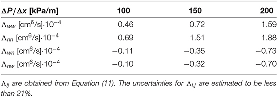
Table 2. Integrated time correlation functions for case (A) and three different settings of the pressure drop across the network.

TABLE 3

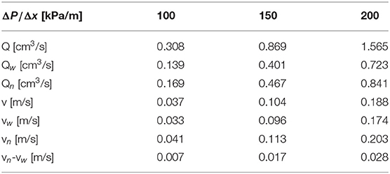
Table 3. Volumetric flow rates Q and fluid velocities v for case (A) and three different settings of the pressure drop across the network.

TABLE 4

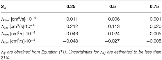
Table 4. Integrated time correlation functions for case (B) and three different choices for the saturation.

TABLE 5

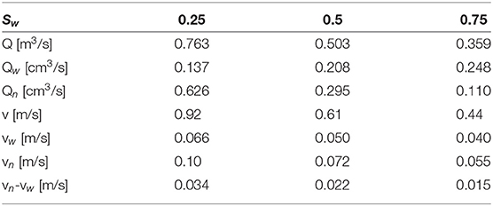
Table 5. Volumetric flow rates Q and fluid velocities v for case (B) and three different choices for the saturation.

In both cases (A) and (B), we find that the integral cross-correlations obey the Onsager reciprocal relation, Λ_ij = Λ_ji, within the statistical error in the simulations. This result is new for a meso-level description like the one used here and is encouraging for the overall aim; to create a non-equilibrium thermodynamic description for the macroscopic level. The finding applies to a well-defined REV, for which we have a Gaussian distribution of fluctuations, analogous to the corresponding distribution on the molecular level.

It is interesting that the cross coefficients are all negative. This makes sense for network flow, where one component cannot advance faster (on average) than the mean flow unless the other component advances slower (on average).

The Λ_ijs for case (B), where the surface tension is zero, show an extreme limit property, because the cross-correlation functions obey Λ_wwΛ_nn − Λ_wnΛ_nw ≈ 0. A singular matrix of coefficients is the essence of complete coupling of the two fluids' flows; they are linearly dependent. For all choices of saturation, ${\Lambda }_{ww}={\zeta }^2{\Lambda }_{nw}$, where ζ is a constant [14]. On the other hand, for case (A), where the surface tension differs from zero, a deviation of this dependency is observed. The linear dependence of the fluxes in case (B) can thus be associated with a lack of capillary forces. This can be understood in the following way: in case (B), the variation of mobility in a given link is a function of the saturation in the link only. However, if the mobility in one link is increased, it has to decrease elsewhere. In contrast, for case (A), the variations in link mobility depend on the interface position, and a change in the link mobility can take place without affecting the mobilities of other links.

The value of ζ for case (B) can be deduced by looking at the coefficients in Table 4. Within the accuracy, we find ζ² ≈ 20 or ζ = 4.5 ± 0.5 for all S_w. The value is close to the ratio of fluid viscosities, which will describe the dissipation.

All coefficients in Table 4 show a dependence on the saturation, decreasing in value as the saturation increases. Here, the wetting fluid is the more viscous fluid, and the increase in saturation reduces the effective permeability. The coefficients also show a dependence on the pressure drops across the network (see Table 2), increasing with higher pressure drops. This is consistent with a higher effective permeability at higher pressures. In fact, the dependence of the volumetric flow is non-linear, as can be seen in Table 3. A non-linear dependence of a flow rate on the pressure difference is a well-known phenomenon in immiscible two-phase flow[29].

To investigate the origin of the Onsager symmetry in more detail, we examined the cross-correlations in Figure 9. For molecular systems, one can find transport coefficients using the Green–Kubo method (see [30]), and Onsager reciprocal relations apply given time-reversal invariance. We have found that time-reversal invariance also applies on the mesoscopic level, as formulated by: C_AB(τ) = C_BA(τ). This equality is illustrated in Figure 9. There is agreement except for values at very short timescales, where the contribution to the integral is negligible. Moreover, for case (B), the deviation from symmetry at small time values is attributable to the finite system size. It vanishes for larger network sizes. This is shown in the upper three panels of Figure 9.

FIGURE 9

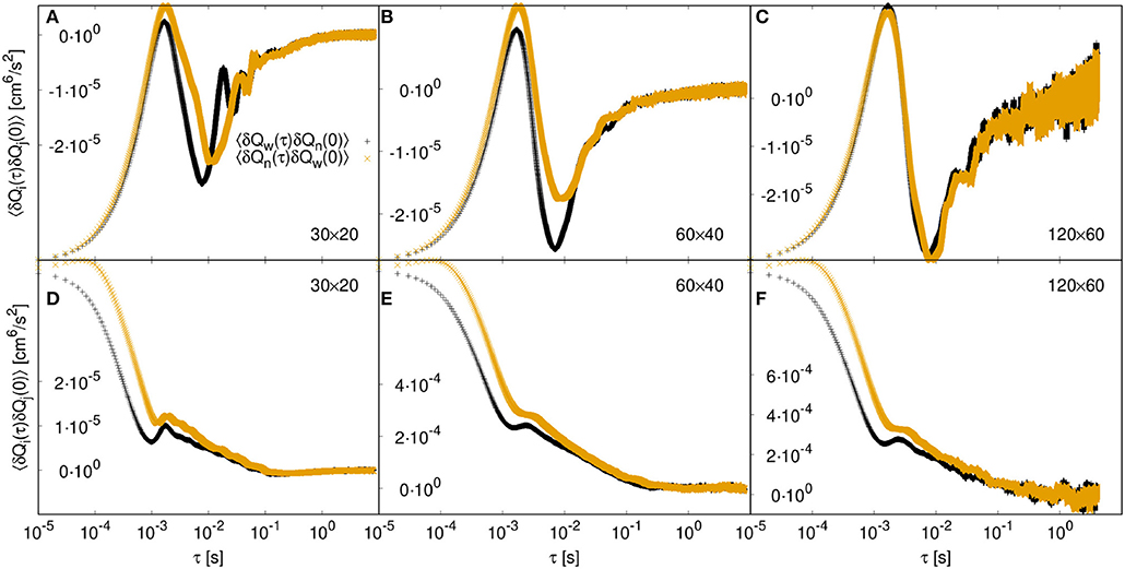
Figure 9. Cross-correlation functions of wetting (Q_w) and non-wetting (Q_n) flows. The upper panels (A–C) show the cross-correlations for case (B) with zero surface tension and increasing network size from (A) to (C). The lower panels (D–F) show the cross-correlations for case (A) with γ = 30 mN/m. The network size is increasing from left to right from 30 × 20 to 60 × 40 to 120 × 60 links.

4. Conclusions

Our investigation of time correlation functions has revealed interesting parallels between the time correlation functions of two immiscible fluids in a porous media, those observed for glass and stress-yield fluids, and those for molecular fluctuations. A network with incompressible fluids has been used as a model for the porous medium, but the findings should not be restricted to this. We have been able for the first time to find Onsager symmetry in athermal fluctuations on the meso level. The symmetry of the coefficients implies time-reversal invariance or microscopic reversibility of fluctuations also on the meso level, in agreement with recent experimental [11] and computational evidence [12, 13]. Time-reversal invariance is here understood as C_AB(τ) = C_BA(τ), holding for all timescales except very short timescales.

We found that the structure of the time correlation functions depends on the surface tension. Integrals over auto- and cross-correlation functions of an REV were found to converge, and the integrals of the cross-correlation functions essentially obeyed Onsager's symmetry. The coefficients obtained in this manner may have a relation to porous medium permeabilities. Further research on time correlation functions to compute the transport properties of immiscible-two phase flow is therefore encouraged.

One may ask whether the dynamic pore network model we have used really reflects the dynamics of real porous media or whether ergodicity has been built into it somehow, ergodicity that is not there in real porous media. Apart from doing experiments that will answer this question, one may repeat the measurements here but based on other models that differ substantially from ours, such as the Lattice Boltzmann Method.

Data Availability Statement

The datasets generated for this study are available on request to the corresponding author.

Author Contributions

MW conceptualized the study, carried out the simulation, and wrote the first draft. MG assisted with the computational work. All authors contributed to data analysis, and in developing the theory as well as shaping the manuscript to its final form.

Funding

This work was supported by the Research Council of Norway through its Centres of Excellence funding scheme, project number 262644. MW is grateful for a postdoc scholarship from the Department of Physics, the Norwegian University of Science and Technology, NTNU, Trondheim.

Conflict of Interest

The authors declare that the research was conducted in the absence of any commercial or financial relationships that could be construed as a potential conflict of interest.

Acknowledgments

The authors would like to thank Prof. Daan Frenkel for helpful discussions of this work. We thank the reviewers for providing us with exceptionally good and challenging reviews.

References

1. Ben-Isaac E, Park Y, Popescu G, Brown FLH, Gov NS, Shokef Y. Effective temperature of red-blood-cell membrane fluctuations. Phys Rev Lett. (2011) 106:238103. doi: 10.1103/PhysRevLett.106.238103

PubMed Abstract | CrossRef Full Text | Google Scholar

2. Gnoli A, Petri A, Dalton F, Pontuale G, Gradenigo G, Sarracino A, et al. Brownian ratchet in a thermal bath driven by coulomb friction. Phys Rev Lett. (2013) 110:120601. doi: 10.1103/PhysRevLett.110.120601

PubMed Abstract | CrossRef Full Text | Google Scholar

3. Bi D, Henkes S, Daniels KE, Chakraborty B. The statistical physics of athermal materials. Annu Rev Condens Matter Phys. (2015) 6:63–83. doi: 10.1146/annurev-conmatphys-031214-014336

CrossRef Full Text |Google Scholar

4. Kanazawa K, Sano TG, Sagawa T, Hayakawa H. Minimal Model of stochastic athermal systems: origin of non-gaussian noise. Phys Rev Lett. (2015) 114:090601. doi: 10.1103/PhysRevLett.114.090601

PubMed Abstract | CrossRef Full Text | Google Scholar

5. Clewett JPD, Wade J, Bowley RM, Herminghaus S, Swift MR, Mazza MG. The minimization of mechanical work in vibrated granular matter. Sci Rep. (2016) 6:28726. doi: 10.1038/srep28726

PubMed Abstract | CrossRef Full Text | Google Scholar

6. Weber SC, Spakowitz AJ, Theriot JA. Nonthermal ATP-dependent fluctuations contribute to the in vivo motion of chromosomal loci. Proc Natl Acad Sci USA. (2012) 109:7338–43. doi: 10.1073/pnas.1119505109

PubMed Abstract | CrossRef Full Text | Google Scholar

7. Dabelow L, Bo S, Eichhorn R. Irreversibility in active matter systems: fluctuation theorem and mutual information. Phys Rev X. (2019) 9:021009. doi: 10.1103/PhysRevX.9.021009

CrossRef Full Text | Google Scholar

8. Kumar N, Soni H, Ramaswamy S, Sood AK. Flocking at a distance in active granular matter [Journal Article]. Nat Commun. (2014) 5:4688. doi: 10.1038/ncomms5688

CrossRef Full Text | Google Scholar

9. Tang H, Yan B, Chai Z, Zuo L, Killough J, Sun Z. Analyzing the well-interference phenomenon in the eagle ford shale/austin chalk production system with a comprehensive compositional reservoir model. SPE Reserv Eval Eng. (2019) 22:827–41. doi: 10.2118/191381-PA

CrossRef Full Text | Google Scholar

10. de Groot SR, Mazur P. Non-equilibrium Thermodynamics. New York, NY: Dover (1984).

Google Scholar

11. Erpelding M, Sinha S, Tallakstad KT, Hansen A, Flekkøy EG, Måløy KJ. History independence of steady state in simultaneous two-phase flow through two-dimensional porous media. Phys Rev E. (2013) 88:053004. doi: 10.1103/PhysRevE.88.053004

PubMed Abstract | CrossRef Full Text | Google Scholar

12. Savani I, Sinha S, Hansen A, Bedeaux D, Kjelstrup S, Vassvik M. A Monte Carlo algorithm for immiscible two-phase flow in porous media. Transport Porous Med. (2017) 116:869–88. doi: 10.1007/s11242-016-0804-x

CrossRef Full Text | Google Scholar

13. Savani I, Bedeaux D, Kjelstrup S, Vassvik M, Sinha S, Hansen A. Ensemble distribution for immiscible two-phase flow in porous media. Phys Rev E. (2017) 95:023116. doi: 10.1103/PhysRevE.95.023116

PubMed Abstract | CrossRef Full Text | Google Scholar

14. Kjelstrup S, Bedeaux D. Non-Equilibrium Thermodynamics of Heterogeneous Systems. World Scientific (2008) Available online at: https://www.worldscientific.com

Google Scholar

15. Onsager L. Reciprocal relations in irreversible processes. I. Phys Rev. (1931) 37:405–26. doi: 10.1103/PhysRev.37.405

CrossRef Full Text | Google Scholar

16. Onsager L. Reciprocal relations in irreversible processes. II. Phys Rev. (1931) 38:2265–79. doi: 10.1103/PhysRev.38.2265

CrossRef Full Text | Google Scholar

17. Flekkøy EG, Pride SR, Toussaint R. Onsager symmetry from mesoscopic time reversibility and the hydrodynamic dispersion tensor for coarse-grained systems. Phys Rev E. (2017) 95:022136. doi: 10.1103/PhysRevE.95.022136

PubMed Abstract | CrossRef Full Text | Google Scholar

18. Aker E, Jørgen Måløy K, Hansen A, Batrouni GG. A two-dimensional network simulator for two-phase flow in porous media. Transport Porous Med. (1998) 32:163–86. doi: 10.1023/A:1006510106194

CrossRef Full Text | Google Scholar

19. Aker E, Måløy KJ, Hansen A, Basak S. Burst dynamics during drainage displacements in porous media: Simulations and experiments. Eur Phys Lett. (2000) 51:55–61. doi: 10.1209/epl/i2000-00331-2

CrossRef Full Text | Google Scholar

20. Zhao B, MacMinn CW, Primkulov BK, Chen Y, Valocchi AJ, Zhao J, et al. Comprehensive comparison of pore-scale models for multiphase flow in porous media. Proc Natl Acad Sci USA. (2019) 116:13799–806.

PubMed Abstract | Google Scholar

21. Flekkøy EG, Pride SR. Reciprocity and cross coupling of two-phase flow in porous media from Onsager theory. Phys Rev E. (1999) 60:4130–7. doi: 10.1103/PhysRevE.60.4130

PubMed Abstract | CrossRef Full Text | Google Scholar

22. Sinha S, Gjennestad MA, Vassvik M, Hansen A. A dynamic network simulator for immiscible two-phase flow in porous media. arXiv e-prints arXiv:1907.12842 (2019).

Google Scholar

23. Sinha S, Bender AT, Danczyk M, Keepseagle K, Prather CA, Bray JM, et al. Effective rheology of two-phase flow in three-dimensional porous media: experiment and simulation. Transport Porous Med. (2017) 119:77–94. doi: 10.1007/s11242-017-0874-4

PubMed Abstract | CrossRef Full Text | Google Scholar

24. Gjennestad MA, Vassvik M, Kjelstrup S, Hansen A. Stable and efficient time integration of a dynamic pore network model for two-phase flow in porous media. Front Phys. (2018) 6:56. doi: 10.3389/fphy.2018.00056

CrossRef Full Text | Google Scholar

25. Sinha S, Gjennestad MA, Vassvik M, Winkler M, Hansen A, Flekkøy EG. Rheology of high-capillary number two-phase flow in porous media. Front Phys. (2019) 7:65. doi: 10.3389/fphy.2019.00065

CrossRef Full Text | Google Scholar

26. Kjelstrup S, Bedeaux D, Hansen A, Hafskjold B, Galteland O. Non-isothermal transport of multi-phase fluids in porous media. Constitutive equations. Front Phys. (2019) 6:150. doi: 10.3389/fphy.2018.00150

CrossRef Full Text | Google Scholar

27. Reichman DR, Charbonneau P. Mode-coupling theory. J Stat Mech Theory Exp. (2005) 2005:P05013. doi: 10.1088/1742-5468/2005/05/p05013

CrossRef Full Text | Google Scholar

28. Levashov VA. Contribution to viscosity from the structural relaxation via the atomic scale Green-Kubo stress correlation function. J Chem Phys. (2017) 147:184502. doi: 10.1063/1.4991310

PubMed Abstract | CrossRef Full Text | Google Scholar

29. Longeron DG. Influence of very low interfacial tensions on relative permeability. Soc Petrol Eng J. (1980) 20:391–401. doi: 10.2118/7609-PA

CrossRef Full Text | Google Scholar

30. Liu X, Schnell SK, Simon JM, Krüger P, Bedeaux D, Kjelstrup S, et al. Diffusion coefficients from molecular dynamics simulations in binary and ternary mixtures. Int J Thermophys. (2013) 34:1169–96. doi: 10.1007/s10765-013-1482-3

CrossRef Full Text | Google Scholar