Effective Rheology of Bi-viscous Non-newtonian Fluids in Porous Media

We model the flow of bi-viscous non-Newtonian fluids in porous media by a square lattice where the links obey a piece-wise linear constitutive equation. We find numerically that the flow regime, where the network transitions from all links behaving according to the first linear part of the constitutive equation to all links behaving according to the second linear part of the constitutive equation, is characterized by a critical point. We measure two critical exponents associated with this critical point, one of them being the correlation length exponent. We find that both critical exponents depend on the parameters of the model.

1. Introduction

The behavior of complex fluids when being inside a porous medium may be very different from that when they are not. This is a problem encountered in many biological or industrial applications ranging from impregnation of fibrous materials to immiscible multi-phase flow in porous media. Among the different types of non-Newtonian fluids, many undergo behavioral changes depending on the stress or strain applied. One can mention the Carreau rheology which is Newtonian at low shear rate but behaves as a power law fluid above a certain shear rate [1]. Other examples are yield stress fluid that responds as a solid below a critical yield threshold. Above, they behave as a power law fluid [2]. At the mesoscopic level, this rheological approach can also be extended to other situations. For example, inertial effects can be described as a rheological change from a Newtonian fluid to a power law (quadratic or cubic) for a given large Reynolds number [3]. Another possible extension is the displacement of immiscible fluids in porous media. In this case, the fluids may each be Newtonian. However, the interfacial tension between them makes them effectively behave in a non-Newtonian way inside the porous medium [4]. Indeed, a non-zero amount of stress is then required for a non-wetting phase to invade the smaller pore throats.

Non-Newtonian fluids are notoriously difficult to treat analytically and computationally. When in addition the flow is constrained by the very complex boundary conditions of a porous medium, the effective rheology of the fluid flow is not well understood. This might for example be seen in the fact that the leading theory for describing immiscible multi-phase flow in porous media is still the relative permeability theory dating from 1936 [5] a theory which has evident weaknesses.

The purpose of this manuscript is to investigate the coupling between the heterogeneity of the medium and a rheology with a change of behavior. We study a very simple model, namely a bi-viscous fluid, where the fluid is Newtonian but with a change of viscosity at one particular shear rate (or shear stress) [6, 7]. The second viscosity might be lower (shear thinning) or higher (shear thickening). As we shall see, the coupling between the disorder and such a simple rheological model is enough to generate a rich problem.

We also choose a simple porous medium; a square lattice oriented at 45° with respect to the average flow direction, see Figure 1, consisting of N_x links in the flow direction and N_y links in the direction orthogonal to the flow direction.

FIGURE 1

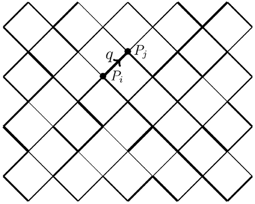
Figure 1. Diamond lattice used in this work. At each node, a pressure P_i is defined. In each link, the flow rate is a function of the pressure difference δP = P_i − P_j according to a bi-viscous model.

The constitutive equation for the fluid in a link in the lattice is given by

$\begin{array}{ll}q(\nabla p)=\{\begin{array}{ll}-\alpha \nabla p\hfill & :|q|\le q_c,\hfill \\ -\beta \nabla p+\text{sgn}(q)\left[1-\frac{\beta }{\alpha }\right]q_c\hfill & :q_c\le |q|,\hfill \end{array}& (1)\end{array}$

where q is the volumetric flow rate in the link, and ∇p is the pressure drop across the link. There are three parameters, α, β and q_c. The two first parameters, α and β are the mobilities when the fluid is either in the “α-mode” or in the “β-mode.” The third parameter, q_c is the flow rate at which the fluid changes from being in α-mode to β-mode. We illustrate the constitutive equation in Figure 2. To simplify the problem as much as possible, we let the two the α-mobilities and the β-mobilities be the same for all links in the lattice. However, each link has its own flow rate threshold q_c drawn from a distribution p(q_c).

FIGURE 2

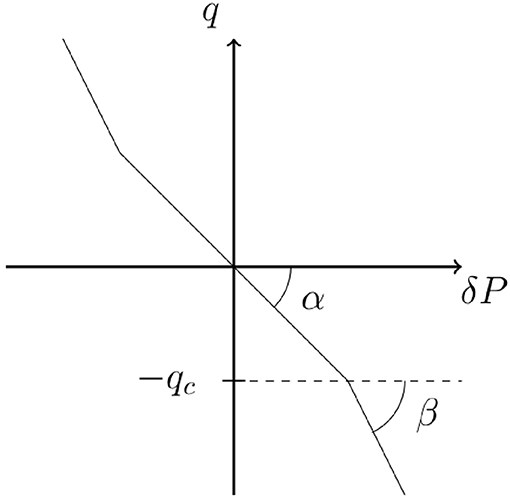
Figure 2. Bi-viscous flow curve. If the absolute value of the flow rate is below a local threshold q_c, the flow is linear with a mobility α. Once the absolute value of the flow rate has reached the threshold the evolution is still linear but with different mobility β.

We will in the following study this system for different values of α and β and for two threshold distributions p(q_c); a uniform distribution and an exponential distribution.

In section 2, we consider the symmetries inherent in the system. There are two types of symmetries. The first type is related to what happens to the volumetric flow rate through the system, Q when we scale the system parameters. Using the Euler theorem for homogeneous functions, we are able to write down the most general form of the volumetric flow rate. If we define 〈q〉 as Q/N_y, where N_y is the width of the lattice in terms of nodes, we find that $\langle q\rangle =\alpha \overline{q}(\nabla p,\beta /\alpha ,\left\{q_c\right\}/\alpha )$, where {q_c} refers to the set of thresholds, one for each link. The second type of symmetry is the self-duality of the square lattice leading to a mapping between the behavior of the system for a given ratio β/α and its inverse, α/β. Hence, we only need to discuss parameters for which β/α ≥ 1, see Figure 3.

FIGURE 3

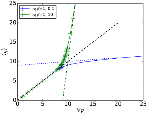
Figure 3. Example of the mean flow rate 〈q〉 as function of the mean gradient ∇p for two different bi-viscous model (α, β) = (1, 10) (blue) and (α, β) = (1, 0.1) (green). As described in the text, the two cases are symmetrical through a duality mapping.

We study in section 3 the lattice with N_x = 1, i.e., there is only one layer. The model then becomes the capillary fiber bundle model which is analytically tractable. We find that for the uniform threshold distribution, the flow rate behaves as $\langle q\rangle -\langle q_c\rangle ~{(\nabla p-\nabla p_c)}^2$ where (〈q_c〉, ∇p_c) is a point only dependent on the value of the ratio β/α and the limits of the uniform distribution q_min and q_max. This is reminiscent of a critical point. However, it is not a critical point. There are no correlations developing in the system as ∇p approaches ∇p_c. Furthermore, the power law behavior is not seen when the threshold distribution is exponential.

Section 4 is devoted to the numerical algorithm we use to solve the flow patterns. Our algorithm is based on the augmented Lagrangian algorithm, which we describe in this section.

We present our results in section 5. First we note that the two limits β/α → 1 and β/α → ∞, or equivalently, β/α → 0 correspond to the directed percolation [8] and the directed polymer problems respectively [9]. This points us in the direction of there being a critical point in the problem in spite of the conclusion drawn for the capillary fiber bundle model in section 3. Indeed, this is what we find, i.e., that $\langle q\rangle -\langle q_c\rangle ~{(\nabla p-\nabla p_c)}^{\mu }$ where μ depends on the ratio β/α for the same type of threshold distribution that gave a power law dependence in the capillary fiber bundle model studied in section 3. We define and measure a correlation length $L_{max}~{(\nabla p-\nabla p_c)}^{-\nu }$. The correlation length exponent ν also depends on the ratio β/α. In the limit β/α → 1, the longitudinal directed percolation correlation length exponent ν_∥ = 1.733847(6) [10] is expected and our numerical results are consistent with this. In the directed polymer limit β/α → ∞, however, the corresponding correlation length exponent is not the usual one, ν_∥ = 3/2 [11], but rather one that describes a correlated directed percolation problem.

The last section 6 contains our summary and conclusions.

2. Symmetries

In this section, we discuss the symmetries that lie hidden in the system we study, a diamond lattice of links obeying the constitutive (Equation 1). We consider two types of symmetry: one is based on scaling of the size and parameters of the model. Through the Euler theorem for homogeneous functions, we are able to write down the most general functional form the volumetric flow rate through the network takes. We then go on to exploring the geometrical symmetry inherent in the diamond lattice due to self-duality in the same way as first done by Straley [12]. This symmetry demonstrates that we only need to explore the part of parameter space for which β/α ≥ 1.

2.1. Scaling Symmetry

The volumetric flow rate Q shows a number of scaling symmetries. We combine these with the Euler theorem for homogeneous functions to deduce the functional form of Q = Q(ΔP, α, β, {q_c}, N_x, N_y) [13]. Here {q_c} is the set of thresholds, one for each link in the network. The volumetric flow rate is extensive in the width of the network, N_y. Hence,

$\begin{array}{l}Q(\Delta P,\alpha ,\beta ,\{q_c\},N_x,{\lambda }_y{N}_y)\\ ={\lambda }_{y}Q(\Delta P,\alpha ,\beta ,\{q_c\},N_x,N_y).& (2)\end{array}$

With respect to the length of the system, we find the symmetry

$\begin{array}{l}Q(\Delta P,\alpha ,\beta ,\{q_c\},N_x,N_y)\\ =Q({\lambda }_x\Delta P,\alpha ,\beta ,\{q_c\},{\lambda }_x{N}_x,N_y).& (3)\end{array}$

A more subtle scaling symmetry is

$\begin{array}{l}Q(\Delta P,{\lambda }_q\alpha ,{\lambda }_q\beta ,\{{\lambda }_q{q}_c\},N_x,N_y)\\ ={\lambda }_{q}Q(\Delta P,\alpha ,\beta ,\{q_c\},N_x,N_y).& (4)\end{array}$

We also have the scaling symmetry

$\begin{array}{l}Q\left(\Delta P,\alpha ,\beta ,\left\{q_c\right\},N_x,N_y\right)\\ =Q\left({\lambda }_P\Delta P,\frac{\alpha }{{\lambda }_P},\frac{\beta }{{\lambda }_P},\{q_c\},N_x,N_y\right).& (5)\end{array}$

The length N_x and width N_y of the network are discrete variables. By setting λ_y = 1/N_y we find from Equation (2) that

$\begin{array}{l}Q(\Delta P,\alpha ,\beta ,\{q_c\},N_x,N_y)\\ =N_{y}Q(\Delta P,\alpha ,\beta ,\{q_c\},N_x,1).& (6)\end{array}$

The second scaling relation, Equation (3) gives when setting λ_x = 1/N_x,

$\begin{array}{l}Q(\Delta P,\alpha ,\beta ,\{q_c\},N_x,N_y)\\ =Q(\nabla p,\alpha ,\beta ,\{q_c\},1,N_y),& (7)\end{array}$

where we have used the definition ∇p = ΔP/N_x. We now combine (Equations 6 and 7) to get

$\begin{array}{l}Q(\Delta P,\alpha ,\beta ,\{q_c\},N_x,N_y)\\ =N_{y}Q(\nabla p,\alpha ,\beta ,\{q_c\},1,1)=\langle q\rangle .& (8)\end{array}$

Hence, we define the average flow rate in the links as

$\begin{array}{ll}\langle q\rangle (\nabla p,\alpha ,\beta ,\{q_c\})=Q(\nabla p,\alpha ,\beta ,\{q_c\},1,1).& (9)\end{array}$

This is thus an intensive variable with respect to the width and the length of the network.

The two remaining scaling relations (4) and (5) involve continuous variables and we may thus make use of Euler's theorem for homogeneous functions. The Euler theorem is easy to implement for each of these four scaling symmetries: we take the derivative with respect to the scaling variable λ in each expression and set the variable equal to one.

The scaling relation (4) gives

$\begin{array}{l}Q(\Delta P,\alpha ,\beta ,\{q_c\},N_x,N_y)\\ =\left(\frac{\partial Q}{\partial \alpha }\right)\alpha +\left(\frac{\partial Q}{\partial \beta }\right)\beta +{\displaystyle \sum _{\text{links}}\left(\frac{\partial Q}{\partial q_c}\right)}{q}_c,& (10)\end{array}$

or in terms of the intensive variable

$\begin{array}{l}\langle q\rangle (\nabla P,\alpha ,\beta ,\{q_c\})\\ =\left(\frac{\partial \langle q\rangle }{\partial \alpha }\right)\alpha +\left(\frac{\partial \langle q\rangle }{\partial \beta }\right)\beta +{\displaystyle \sum _{\text{links}}\left(\frac{\partial \langle q\rangle }{\partial q_c}\right)}{q}_c.& (11)\end{array}$

We define the functions

$\begin{array}{ll}A=-\left(\frac{\partial \langle q\rangle }{\partial \alpha }\right),& (12)\end{array}$

$\begin{array}{ll}B=-\left(\frac{\partial \langle q\rangle }{\partial \beta }\right),& (13)\end{array}$

and,

$\begin{array}{ll}\left\{c\right\}=\left\{\left(\frac{\partial \langle q\rangle }{\partial q_c}\right)\right\}.& (14)\end{array}$

There is one function c for each link in the network.

Whereas 〈q〉 is homogeneous of order one¹ in the variables α, β and {q_c}, the functions A, B and {c} are homogeneous of order zero in these variables. This means that the parameters α, β and {q_c} only appear as ratios in these functions,

$\begin{array}{ll}A=A\left(\nabla p,\frac{\beta }{\alpha },\frac{\left\{q_c\right\}}{\alpha }\right),& (15)\end{array}$

$\begin{array}{ll}B=B\left(\nabla p,\frac{\beta }{\alpha },\frac{\left\{q_c\right\}}{\alpha }\right),& (16)\end{array}$

and

$\begin{array}{ll}\left\{c\right\}=\left\{c\left(\nabla p,\frac{\beta }{\alpha },\frac{\left\{q_c\right\}}{\alpha }\right)\right\}.& (17)\end{array}$

Equation (10) may thus be written

$\begin{array}{l}\langle q\rangle (\nabla P,\alpha ,\beta ,\{q_c\})=\\ -A\left(\nabla p,\frac{\beta }{\alpha },\frac{\left\{q_c\right\}}{\alpha }\right)\alpha -B\left(\nabla p,\frac{\beta }{\alpha },\frac{\left\{q_c\right\}}{\alpha }\right)\beta \\ +{\displaystyle \sum _{\text{links}}c}\left(\nabla p,\frac{\beta }{\alpha },\frac{\left\{q_c\right\}}{\alpha }\right)q_c.& (18)\end{array}$

Scaling Equation (5) combined with the Euler theorem gives

$\begin{array}{ll}\left(\frac{\partial Q}{\partial \Delta P}\right)\Delta P=\left(\frac{\partial Q}{\partial \alpha }\right)\alpha +\left(\frac{\partial Q}{\partial \beta }\right)\beta ,& (19)\end{array}$

In terms of 〈q〉 and Equation (17), we may rewrite this Equation

$\begin{array}{l}m\left(\nabla p,\frac{\beta }{\alpha },\frac{\left\{q_c\right\}}{\alpha }\right)\nabla p\\ =A\left(\nabla p,\frac{\beta }{\alpha },\frac{\left\{q_c\right\}}{\alpha }\right)\alpha \\ +B\left(\nabla p,\frac{\beta }{\alpha },\frac{\left\{q_c\right\}}{\alpha }\right)\beta ,& (20)\end{array}$

where we have defined the mobility

$\begin{array}{ll}m=-\left(\frac{\partial \langle q\rangle }{\partial \nabla p}\right).& (21)\end{array}$

From Equations (10) and (19), we deduce that

$\begin{array}{ll}\langle q\rangle =\left(\frac{\partial \langle q\rangle }{\partial \nabla p}\right)\nabla p+{\displaystyle \sum _{\text{links}}}c{q}_c=-m\nabla p+{\displaystyle \sum _{\text{links}}}c{q}_c,& (22)\end{array}$

and with the help of Equation (20) we find

$\begin{array}{l}\langle q\rangle =-a\left(\nabla p,\frac{\beta }{\alpha },\frac{\left\{q_c\right\}}{\alpha }\right)\alpha \nabla p\\ -b\left(\nabla p,\frac{\beta }{\alpha },\frac{\left\{q_c\right\}}{\alpha }\right)\beta \nabla p\\ +{\displaystyle \sum _{\text{links}}c}\left(\nabla p,\frac{\beta }{\alpha },\frac{\left\{q_c\right\}}{\alpha }\right)q_c,& (23)\end{array}$

where we have defined

$\begin{array}{ll}a\left(\nabla p,\frac{\beta }{\alpha },\frac{\left\{q_c\right\}}{\alpha }\right)\nabla p=A\left(\nabla p,\frac{\beta }{\alpha },\frac{\left\{q_c\right\}}{\alpha }\right),& (24)\end{array}$

and,

$\begin{array}{ll}b\left(\nabla p,\frac{\beta }{\alpha },\frac{\left\{q_c\right\}}{\alpha }\right)\nabla p=B\left(\nabla p,\frac{\beta }{\alpha },\frac{\left\{q_c\right\}}{\alpha }\right).& (25)\end{array}$

We may take Equation (23) one step further by dividing out the parameter α,

$\begin{array}{ll}\frac{\langle q\rangle }{\alpha }=\overline{q}\left(\nabla p,\frac{\beta }{\alpha },\frac{\left\{q_c\right\}}{\alpha }\right),& (26)\end{array}$

where,

$\begin{array}{l}\overline{q}\left(\nabla p,\frac{\beta }{\alpha },\frac{\left\{q_c\right\}}{\alpha }\right)=\\ -a\left(\nabla p,\frac{\beta }{\alpha },\frac{\left\{q_c\right\}}{\alpha }\right)\nabla p\\ -b\left(\nabla p,\frac{\beta }{\alpha },\frac{\left\{q_c\right\}}{\alpha }\right)\frac{\beta }{\alpha }\nabla p\\ +{\displaystyle \sum _{\text{links}}c}\left(\nabla p,\frac{\beta }{\alpha },\frac{\left\{q_c\right\}}{\alpha }\right)\frac{q_c}{\alpha }.& (27)\end{array}$

We may as a check, compare Equation (23)—our main result in this section—with the constitutive Equation (1) in the case when there is no disorder, i.e., when all q_c are equal. In this case, 〈q〉 should be equal to the constitutive equation. Hence, in this case we find,

$\begin{array}{ll}a\left(\nabla p,\frac{\beta }{\alpha }\right)=\Theta (q_c-|q|),& (28)\end{array}$

$\begin{array}{ll}b\left(\nabla p,\frac{\beta }{\alpha }\right)=\Theta (|q|-q_c),& (29)\end{array}$

and

$\begin{array}{ll}c\left(\nabla p,\frac{\beta }{\alpha }\right)=\Theta (|q|-q_c)\text{ sign}(q)\left(1-\frac{\beta }{\alpha }\right).& (30)\end{array}$

Here Θ is the Heaviside step function which is one for positive arguments and zero for negative arguments. We note that if |q| < q_min, then Equations (28–30) are correct as the disorder is not “noticeable” in this flow regime.

2.2. Self-Duality of the Square Lattice

We define a dual network as sketched in Figure 4. A node is located at the center of each cell and there is a link connecting each adjacent cell. On each link, a “dual” current is defined from the pressure difference between pressure by the crossed link (from the original network),

$\begin{array}{l}{j}_{A\to B}=P_1-P_4,\\ j_{A\to D}=P_2-P_1,\\ j_{F\to A}=P_3-P_4,\\ j_{E\to A}=P_2-P_3.& (31)\end{array}$

The current in the dual lattice satisfies the conservation of mass at each node (e.g., the Kirchhoff condition) since j_A→B + j_A→D − j_F→A − j_E→A = 0.

FIGURE 4

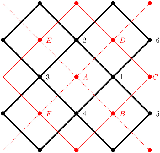
Figure 4. Sketch of the dual network construction. From the original network (black), one can construct a dual one (red), where the nodes are located at the center of the original cells. At each link of the dual network we associate a “dual” flow rate obtained from the pressure difference of the original network. At each node we associate a “dual” pressure based on the original flow rate. See the text for details.

Moreover, one can define a pressure field W on the dual lattice defined from this gradient,

$\begin{array}{l}{W}_A-W_B=q_{1\to 4},\\ W_B-W_C=q_{1\to 5},\\ W_C-W_D=q_{1\to 6},\\ W_D-W_A=q_{1\to 2}.& (32)\end{array}$

The definition is consistent once W is defined at a single point since the sum over a closed loop (and thus any) is equal to zero, (W_A − W_B) + (W_B − W_C) + (W_C − W_D) + (W_D − W_A) = q_1→4 + q_1→5 + q_1→6 + q_1→2 = 0.

Hence, the “dual” pressure gradient and current follow the constitutive equation,

$\begin{array}{ll}{W}_A-W_B=q_{1\to 4}=q(P_A-P_B)=q(j_{A\to B}),& (33)\end{array}$

so that,

$\begin{array}{ll}{j}_{A\to B}=q^{-1}(W_A-W_B).& (34)\end{array}$

Hence, the dual pressure and flow rate field satisfy the same kind of equation but with a local law which is inverted. It is important to note that the mean flow in the dual lattice is perpendicular to the original one.

3. Capillary Fiber Bundle Model

We now consider an analytically solvable model for the flow. Let us assume that the network consists of a set of parallel links placed between two fluid reservoirs kept at pressure p = 0 and p = ∇p < 0, i.e., we are describing the capillary fiber bundle model [14–16]. The constitutive equation for the fiber bundle is then given by

$\begin{array}{l}Q={\displaystyle \sum _{i=1}^{N_y}[-\Theta (q_i-\alpha |\nabla p|)\alpha \nabla p}\\ -\Theta (\alpha |\nabla p|-q_i)\beta \nabla p\\ +\Theta (\alpha |\nabla p|-q_i)\left(1-\frac{\beta }{\alpha }\right)q_i],& (35)\end{array}$

where we have labeled the links according to their position, i = 1, ⋯ , N_y and q_i is the threshold of the ith link.

Let us now relabel the links in ascending order with respect to their thresholds: q₍₁₎ ≤ q₍₂₎ ≤ ⋯ ≤ q_(Ny). Equation (35) then becomes

$\begin{array}{l}Q={\displaystyle \sum _{k=1}^{N_y}[-\Theta (q_{(k)}-\alpha |\nabla p|)\alpha \nabla p}\\ -\Theta (\alpha |\nabla p|-q_{(k)})\beta \nabla p\\ +\Theta (\alpha |\nabla p|-q_{(k)})\left(1-\frac{\beta }{\alpha }\right)q_{(k)}].& (36)\end{array}$

The thresholds are distributed according to the probability distribution p(q_c), with a corresponding cumulative probability given by

$\begin{array}{ll}P(q_c)={\displaystyle {\int }_0^{q_c}}p(q)dq.& (37)\end{array}$

According to order statistics, the mean value of kth largest threshold—mean value in the sense of averaging over an ensemble of networks—is given by

$\begin{array}{ll}P({\overline{q}}_{(k)})=\frac{k}{N_y+1}\approx \frac{k}{N_y}.& (38)\end{array}$

Thus, the ensemble averages of the three types of sums in Equation (36) are then

$\begin{array}{ll}{\displaystyle \sum _{k=1}^{N_y}}\Theta ({\overline{q}}_{(k)}-\alpha |\nabla p|)=N_y\left[1-P(\alpha |\nabla p|)\right],& (39)\end{array}$

$\begin{array}{ll}{\displaystyle \sum _{k=1}^{N_y}}\Theta (\alpha |\nabla p|-{\overline{q}}_{(k)})=N_{y}P(\alpha |\nabla p|),& (40)\end{array}$

and

$\begin{array}{ll}{\displaystyle \sum _{k=1}^{N_y}}\Theta (\alpha |\nabla p|-{\overline{q}}_{(k)}){\overline{q}}_{(k)}=N_y{\displaystyle {\int }_0^{\alpha \nabla p}}p(q)qdq.& (41)\end{array}$

Inserted into Equation (36), these averages give

$\begin{array}{l}\langle q\rangle =-[1-P(\alpha |\nabla p|)]\alpha \nabla p-P(\alpha |\nabla p|)\beta \nabla p\\ +\left[1-\frac{\beta }{\alpha }\right]{\displaystyle {\int }_0^{\alpha |\nabla p|}p}(q)qdq,& (42)\end{array}$

where 〈q〉 = Q/N_y.

3.1. Uniform Threshold Distribution

We now consider the concrete threshold distribution we will also employ in our numerical simulations on the square lattice: a uniform distribution on the interval (q_min, q_max). Hence,

$\begin{array}{ll}p(q_c)=\{\begin{array}{ll}0\hfill & :q_c\le q_{\min },\hfill \\ {(q_{\max }-q_{\min })}^{-1}\hfill & :q_{\min }<q_c<q_{\max },\hfill \\ 0\hfill & :q_{\max }\le q_c,\hfill \end{array}& (43)\end{array}$

We define

$\begin{array}{ll}\nabla p_{min}=-\frac{q_{min}}{\alpha },& (44)\end{array}$

and

$\begin{array}{ll}\nabla p_{max}=-\frac{q_{max}}{\alpha }.& (45)\end{array}$

We also define

$\begin{array}{ll}\nabla p_0=\frac{1}{2}\left[\nabla p_{min}+\nabla p_{max}\right].& (46)\end{array}$

Inserting these expressions into Equation (42) gives

$\begin{array}{ll}\langle q\rangle =\{\begin{array}{ll}-\alpha \nabla p\hfill & :|\nabla p|\le |\nabla p_{\min }|,\hfill \\ \frac{(\alpha -\beta ){(\nabla p-\nabla p_c)}^2}{2(\nabla p_{\max }-\nabla p_{\min })}\hfill & \hfill \\ -\frac{\alpha (\alpha \nabla p_0-\beta \nabla p_{\min })}{\alpha -\beta }\hfill & :|\nabla p_{\min }|<|\nabla p|\hfill \\ \hfill & :|\nabla p|<|\nabla p_{\max }|,\hfill \\ -\beta \nabla p-(\alpha -\beta )\nabla p_0\hfill & :|\nabla p_{\max }|\le |\nabla p|.\hfill \end{array}& (47)\end{array}$

We have here defined

$\begin{array}{ll}\nabla p_c=\frac{\alpha \nabla p_{max}-\beta \nabla p_{min}}{\alpha -\beta }.& (48)\end{array}$

If we now define

$\begin{array}{ll}\langle q_c\rangle =\frac{\alpha (\beta \nabla p_{min}-\alpha \nabla p_0)}{\alpha -\beta },& (49)\end{array}$

we may cast the middle regime where |∇p_min| < |∇p| < |∇p_max| in the form

$\begin{array}{ll}\langle q\rangle =\langle q_c\rangle +\frac{(\alpha -\beta )}{2(\nabla p_{min}-\nabla p_{max})}{(\nabla p-\nabla p_c)}^2.& (50)\end{array}$

It straight forward but somewhat tedious to rewrite the average flow rate 〈q〉, Equation (47) in the general form (26) and (27) resulting from the scaling relations (2) to (5).

3.2. Exponential Threshold Distribution

Let us now consider the exponential threshold distribution

$\begin{array}{ll}p(q_c)=\frac{e^{-q_c/q_0}}{q_0},& (51)\end{array}$

for 0 ≤ q_c < ∞. The corresponding cumulative distribution is

$\begin{array}{ll}P(q_c)=1-e^{-q_c/q_0}.& (52)\end{array}$

Inserted into Equation (42), this gives

$\begin{array}{l}\langle q\rangle =-e^{\alpha \nabla p/q_0}\alpha \nabla p\\ -\left(1-e^{\alpha \nabla p/q_0}\right)\beta \nabla p\\ +\left[1-\frac{\beta }{\alpha }\right]\left[q_0-e^{\alpha \nabla p/q_0}\left(q_0-\alpha \nabla p\right)\right],& (53)\end{array}$

where we are still assuming ∇p < 0. Let us set q₀ = −α∇p. We then have the limits

$\begin{array}{ll}\langle q\rangle =\{\begin{array}{ll}-\alpha \nabla p\hfill & :|\nabla p|\ll q_0/\alpha ,\hfill \\ -\beta \nabla p+(\alpha -\beta /)\nabla p_0\hfill & :q_0/\alpha \ll |\nabla p|.\hfill \end{array}& (54)\end{array}$

In contrast to the uniform distribution discussed in section 3.1, there is not a transitional regime between the two limits of Equation (54) which is on the form (50).

Hence, the uniform distribution on an interval, (43) results in 〈q〉 following a power law in 〈q〉 − 〈q_c〉 vs. ∇p − ∇p_c, Equation (50), whereas the exponential distribution (51) does not. From the simple capillary fiber bundle model we may conclude that the power law behavior seen in Equation (50) is incidental and due to the uniform threshold distribution, which in itself is a power law (with exponent zero).

We study a two-dimensional network mode in section 5. Surprisingly, we find that also in this case, only the uniform distribution leads to a flow dependency on the pressure drop of the form

$\begin{array}{ll}\langle q\rangle -\langle q_c\rangle ~{(\nabla p-\nabla p_c)}^{\mu }.& (55)\end{array}$

In this case, however, the exponent μ depends on the parameter ratio β/α.

4. Numerical Method: Augmented Lagrangian

For completeness, this section describes the numerical method used to solve the non-linear Kirchhoff equations. This section is not required to understand the results that follow.

The method used is based on the Augmented Lagrangian method commonly used to solve the Stokes Equation for yield stress fluids [17, 18]. It is based on a variational approach. We start by rewriting the local Equation (1), introducing the function f(q) as

$\begin{array}{ll}\delta p(q)=-f(q)=\{\begin{array}{ll}-\frac{1}{\alpha }q\hfill & :|q|<q_c\hfill \\ -\frac{1}{\beta }\left[q-\frac{q}{|q|}(1-\frac{\beta }{\alpha })\right]\hfill & :|q|>q_c.\hfill \end{array}& (56)\end{array}$

We define a function $\varphi (q)={\int }_0^{q}f(q^{\prime })d{q}^{\prime }$. The flow field {q_l} solution of Equation (1), with the constraints of imposed inlet and outlet pressures at the boundaries p_in and p_out, can be written as the saddle point of the functional

$\begin{array}{l}\underset{\left\{{\lambda }_n\right\}}{\max }\underset{\left\{q_l\right\}}{\min }\Phi [\{q_l\},\{{\lambda }_n\}]\\ ={\displaystyle \sum _{l\in {L}}\left[\varphi (q_n)-{\delta }_{l,in}{p}_{in}{q}_l+{\delta }_{l,out}{p}_{out}{q}_l\right]}\\ +{\displaystyle \sum _{n\in N}{\lambda }_n}{\displaystyle \sum _{l^{\prime }\in V(n)}{q}_{l^{\prime }}},& (57)\end{array}$

where ${L}$ represents the ensemble of links, ${N}$ the ensemble of nodes and ${V}(n)$ the ensemble of links connected to node n. The symbol δ_l,in (resp. δ_l,out) is equal to 1 if the link is connected to the inlet (resp. outlet) node and to 0 otherwise. The {λ_n} field is a set of Lagrangian multipliers which imposes the conservation of mass at each node (and it may thus be associated to a pressure field).

The main idea of the Augmented Lagrangian method is to introduce a secondary set of velocities {j_l} to decouple the non-linear rheology from the Kirchhoff Equation. Another constraint is then added {j_l} = {q_l} via the Lagrangian method.

Hence, the velocity field is the solution of the equation

$\begin{array}{l}\underset{{}_{\{{\lambda }_n\},\{{\mu }_n\}}}{\max }\underset{{}_{\{q_l\},\{j_l\}}}{\min }\Psi [\{q_l\},\{j_l\},\{{\lambda }_n\},\{{\mu }_l\}]\\ ={\displaystyle \sum _{l\in {L}}[\varphi (q_n)-{\delta }_{l,in}{p}_{in}{j}_l+{\delta }_{l,out}{p}_{out}{j}_l}\\ +\mu (j_l-q_l)+\frac{ϵ}{2}|q_l-j_l{|}^2]\\ +{\displaystyle \sum _{n\in N}{\lambda }_n}{\displaystyle \sum _{l^{\prime }\in V(n)}{j}_{l^{\prime }}},& (58)\end{array}$

where {μ_l} is a set of Lagrangian multipliers. The quadratic term is an additional penalty term which characterizes the augmented Lagrangian approach. Here ϵ is a parameter determining its strength.

The methods consists now in implementing an iterative algorithm to reach the saddle point starting from an initial guess $\left\{q_l^0\right\}$, $\left\{j_l^0\right\}$, $\left\{{\lambda }_n^0\right\}$ and $\left\{{\mu }_l^0\right\}$.

Knowing $\left\{q_l^n\right\}$, $\left\{j_l^n\right\}$, $\left\{{\lambda }_n^n\right\}$ and $\left\{{\mu }_n^n\right\}$, the algorithm is decomposed in the following steps.

Determination of $\{j_l^{n+1}\}$ and $\{{\lambda }_n^{n+1}\}$:

For this step we solve

$\begin{array}{l}\forall l\in {L},\frac{\partial }{\partial j_l}\Psi [\{q_l^n\},\{j_l\},\{{\lambda }_n\},\{{\mu }_l^n\}]=0,\\ \forall n\in {N},\frac{\partial }{\partial {\lambda }_n}\Psi [\{q_l^n\},\{j_l\},\{{\lambda }_n\},\{{\mu }_l^n\}]=0,& (59)\end{array}$

which reads

$\begin{array}{ll}\forall l\in {L},j^{n+1}=-\frac{1}{ϵ}({\lambda }_{l+}^{n+1}-{\lambda }_{l-}^{n+1}+{\mu }_l^n-ϵq_l^n)& (60)\end{array}$

$\begin{array}{ll}\forall n\in {N},{\displaystyle \sum _{l^{\prime }\in {V}(n)}}{j}_{l^{\prime }}^{n+1}=0,& (61)\end{array}$

where ${\lambda }_{l+}^{n+1}$ and ${\lambda }_{l-}^{n+1}$ are the Lagrangian multipliers of the two nodes adjacent to link l. For nodes adjacent to the outlet (resp. inlet), λ₊ (resp. λ₋) has to be replaced with p_out (resp. p_in).

The most important point of this set of equations is that it is equivalent to solving the standard linear Kirchhoff equations with a constant permeability 1/ϵ but with an additional source term ${\mu }_l^n-ϵq_l^n$. Hence, it may be solved by standard linear methods (uch as Cholesky, LU decomposition, etc.).

Determination of $q_l^{n+1}$:

We solve

$\begin{array}{ll}\forall l\in {L},\frac{\partial }{\partial q_l}\text{Ψ}\left[\left\{q_l\right\},\left\{j_l^{n+1}\right\},\left\{{\lambda }_n^{n+1}\right\},\left\{{\mu }_l^n\right\}\right]=0,& (62)\end{array}$

which the local, but implicit equation

$\begin{array}{ll}\forall l\in {L},{\varphi }^{\prime }(q_l^{n+1})+ϵq_l^{n+1}=\mu +ϵj_l^{n+1};.& (63)\end{array}$

Noting that $y=\mu +ϵj_l^{n+1}$, the solution is given by

$\begin{array}{ll}{q}_l^{n+1}=\{\begin{array}{ll}\frac{1}{1/\alpha +ϵ}y\hfill & :|y|<ϵi_c+\frac{i_c}{\alpha },\hfill \\ \frac{1}{1/\beta +ϵ}\left[|y|+(1/\beta -1/\alpha )i_c\right]\text{sign}(\text{y})\hfill & :|y|>ϵi_c+\frac{i_c}{\alpha }.\hfill \end{array}& (64)\end{array}$

Determination of ${\mu }_l^{n+1}$:

For this step, we update in the direction of the gradient (Newton method)

$\begin{array}{ll}{\mu }_l^{n+1}={\mu }_l^{n+1}+\gamma (j_l^{n+1}-q_l^{n+1}),& (65)\end{array}$

where γ is a parameter set to γ = ϵ for simplicity.

In practice, this algorithm is iterated until the relative variation of the total flow rate between two step is below 10⁻⁵%. The computational time and the number of steps are strongly varying depending on β but also on the applied pressure.

5. Results

We now our numerical model based on the network show in Figure 1 and the algorithm described in section 4. We use the link threshold distribution (43) with q_min = 7.5 and q_max = 12.5 in the following.

5.1. Criticality

As noted above, due to the distribution of thresholds, the links will reach their thresholds at different macroscopic pressures. A link l will be defined as being in β-mode if q_l > q_c and in α-mode otherwise. Similar to the percolation problem, a macroscopic change in flow regime is expected once there are percolation pathways of β-mode links. However, it is important to note a major difference with the percolation problem: the mode of a link influences the neighboring links. Indeed, in the case of β > α, once a link switches to β-mode, the flow will be easier through it. This will tend to concentrate the flow toward it. It will therefore increase the flow in the upstream and downstream neighboring links and as a consequence push these links toward the β-mode. In the opposite case, for β < α, the β-mode has a lower conductivity once entering this mode compared to what it would have in α-mode. Flow will therefore tend to go around it, increasing the flow in the other lateral links. Consequently β-mode links will tend to correlate in the stream-wise (or lateral) direction for β > α and orthogonally to the stream-wise direction for β < α [19].

The intermediate case β = α is interesting as the mode of a link has no influence on its neighbors. Since the mobility are the same for every link, the flow rate and the pressure gradient become homogeneous and equal to the mean flow rate and mean gradient. The problem is therefore identical to the directed percolation problem [8].

The other limit β/α ≫ 1, the problem becomes identical to that of a yield stress fluid in a porous medium [9, 20, 21]. The critical path is then related to the directed polymer problem [9, 22–24], as it corresponds to the path that minimizes the sum of local pressure threshold ΔP_c = min∑(q_c/α).

5.2. Pathscape Method

To quantify this phenomenon and to determine the percolation pressure, we determine the longest directed path of the β-mode links. This quantity is essentially the longitudinal correlation length in directed percolation [10]. We map the length of all paths by invoking a pathscape approach as described in Talon et al. [24] for yield-stress fluids.

We introduce the node field L_n representing the longest upstream directed path ending at n. L_n can be determined from a transfer matrix algorithm propagating from left to right (stream direction). If we note, at a given node n, l₁ and l₂ the two upstream neighbor links and n₁ and n₂ the corresponding nodes. We associate binary variables m₁ and m₂ with the two links l₁ and l₂. If link l₁ is in β-mode, then m₁ = 1, otherwise m₁ = 0 — and likewise for the link l₂. We then have that

$\begin{array}{ll}{L}_n=max\left[(L_{n_1}+1)m_1,(L_{n_2}+1)m_2\right].& (66)\end{array}$

We proceed by constructing the node field R_n containing the longest directed path ending at n but propagating in the downstream direction. This algorithm is identical to the previous one but it propagates in the upstream direction from the rightmost column.

Once both fields have been determined, we sum the two to obtain the pathscape T_n = L_n + R_n, which contains the length of longest directed percolating path passing by the node n. From this pathscape, we can then identify the longest directed path L_max = max(T_n). In Figure 5, we present two examples of such a pathscape at two different imposed pressure. We see here the longest cluster path in dark blue. At low applied pressure, the longest cluster is quite low L_max = 7, whereas at higher pressure, L_max is closer to the system size.

FIGURE 5

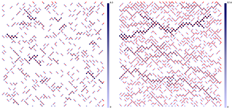
Figure 5. Pathscapes in the network at pressure differences ∇p = 8 (Left) and ∇p = 8.6 (Right). The links in α-mode are not shown. Each link in β-mode have been assigned a color. The color reflects the length of the path to which the link in β-mode belongs, according to the bar to the right of each network. The shortest paths are light blue, the longest are dark blue.

It is important to note that the pathscape we have defined here is not the landscape of minimal paths [24]. In the limit β → α the pathscape reflects the clusters in directed percolation as noted in section 5.1. However, when β ≠ α, the paths we identify correspond to directed percolation clusters. However, the directed percolation is now correlated.

5.3. Evolution of the Correlation Length L_max

In Figure 6, we investigate the evolution of L_max as function of the applied pressure. As it can be seen, the correlation length increases with pressure until it reaches the system length N_x. Similarly to percolation, one can see in Figure 6B that the correlation length diverges as a power law close to a critical pressure gradient ∇p_c,

$\begin{array}{ll}{L}_{max}\propto {(\nabla p_c-\nabla p)}^{-\nu }.& (67)\end{array}$

We note in this figure that the exponent ν seems to vary with β. In Figure 7, we display the evolution of ν and the critical pressure gradient ∇p_c against the parameter β. As we can see, ν and ∇p_c decrease significantly with β. Where the limit β → 1 is consistent with the results found in the literature on directed percolation, ν = ν_∥ = 1.733847(6) [10]. Our best estimate of the threshold pressure is ∇p_c ≈ 10.72.

FIGURE 6

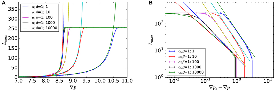
Figure 6. Correlation length L_max as function of the gradient of pressure ∇p (A) or of the distance to the critical pressure |∇p − ∇p_c| (B) for different value of β. The solid line correspond to the power law fit given by Equation (67). The system size is 256 × 256.

FIGURE 7

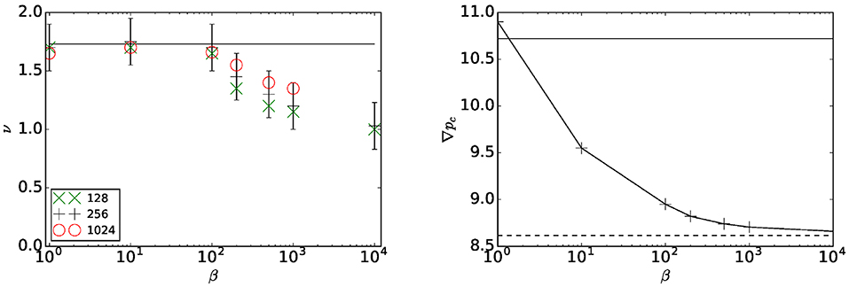
Figure 7. (Left) ν as function of β for system sizes 128 × 128, 256 × 256 and 1, 024 × 1, 024. The data set for L = 128, 256, and 1, 024 are respectively based on 200, 200 and 10 realizations for each value of β. The horizontal line corresponds to the directed percolation exponent ν ≈ 1.72. (Right) Critical gradient of pressure ∇P_c(β) as function of β for the system size 256 × 256. The upper line corresponds to directed percolation (p_c = 0.644700185(5) [10]). The line below (dashed) corresponds to the average of the directed polymer algorithm.

At the end of section 5.2 we noted that the pathscape we have identified is not related to the pathscape spanned by minimal paths in the limit β/α → ∞. If that were the case, we would have expected ν to approach the value ν_∥ = 3/2 [11]. Rather, we are identifying directed percolation clusters in a correlated landscape, and this directed percolation ν is approaching the value 1 in this limit.

5.4. Flow Curve

We now investigate the flow curve. Figure 8 displays the evolution of the mean flow rate as function of the pressure gradient and for different β. In the lower figure, we show that, close to the critical pressure, the flow rate also follows a power-law which can be written on the form

$\begin{array}{ll}\langle q\rangle -{\langle q\rangle }_c\propto {(\nabla p-\nabla p_c)}^{\mu },& (68)\end{array}$

where q_c is a constant obtained by interpolating the data at the critical pressure. We note here that the exponent μ varies with the coefficient β. In Figure 9, we report the evolution of this exponent as a function of 1/log(β). For β = α = 1 we have the obvious limiting value μ = 1. As β increases, so does the value of μ. By plotting μ against 1/log(β) we estimate the limiting value for β → ∞, which is consistent with the value μ = 2; the value suggested by Roux and Herrmann in 1987 [25].

FIGURE 8

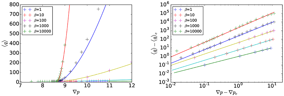
Figure 8. Mean flow rate 〈q〉 as function of the mean pressure gradient (Left) and of the distance to the critical pressure gradient ∇p − ∇p_c (Right) for different β. The solid lines correspond the power law fit given by Equation (68). The system size is 256 × 256.

FIGURE 9

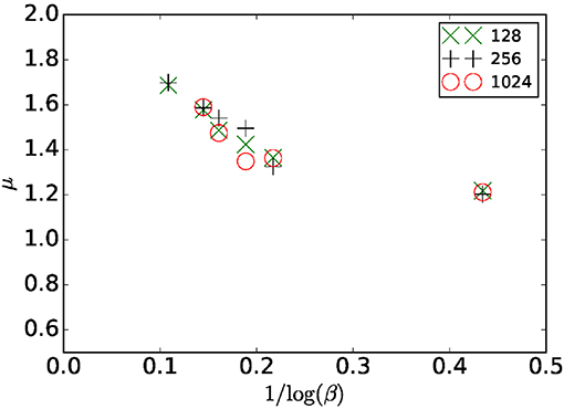
Figure 9. Flow exponent μ as function of 1/log(β) for a system sizes L = 128 × 128, 256 × 256, and 1, 024 × 1, 024. The dependence of the exponent with system size is smaller than the error bars.

We note that the functional form 〈q〉, Equation (68), based on the uniform threshold distribution (43), gives a behavior closely related to the one found for the capillary fiber bundle model with the same type of threshold distribution, see Equation (50), but with μ = 2. The correlation length exponent ν cannot be defined in the capillary fiber bundle model.

In section 3.2, we studied the capillary fiber bundle model with an exponential threshold distribution (51). We have used the same distribution for the network model considered here. As in the capillary fiber bundle model, we do not find a power law of the type (68) in this case, nor do we find a power law for the correlation length (67).

6. Summary and Conclusions

We have explored the behavior of a bi-viscous fluid moving in a diamond lattice subject to the constitutive Equation (1) for each link. This system contains a critical point which leads to the behavior $\langle q\rangle -\langle q_c\rangle ~{(\nabla p-\nabla p_c)}^{\mu }$ for the volumetric flow rate and $L_{max}~{(\nabla p-\nabla p_c)}^{-\nu }$ for the correlation length when a uniform threshold distribution is used. However, the two limits of the ratio between the two parameters representing the mobilities, β/α → 1 and β/α → ∞, or equivalently, β/α → 0 correspond to the percolation and the directed polymer problems respectively. These are problems containing critical points.

There are still a number of open questions concerning this system. We list them as follows:

• We have only considered ∇p ≥ ∇p_c. What happens on the other side of the critical point?

• The critical exponents μ and ν are functions of the parameter ratio β/α. Is this a crossover or are we dealing with non-universal exponents?

• We have only dealt with β ≥ 0. What happens for β < 0 ? The limit β → −∞ turns the model into the fuse model. What happens when β is barely negative? Our numerical algorithm is not capable of handling this problem.

• It would be more realistic, but also more challenging to consider a power-law type characteristic for the constitutive Equation for q ≥ q_c. How will this change our conclusions?

• Why do we not see critical behavior for the exponential threshold distribution in the network model?

Data Availability Statement

All datasets generated for this study are included in the article/supplementary material.

Author Contributions

LT did the numerical computations. AH did the theoretical part. Both authors wrote the paper.

Conflict of Interest

The authors declare that the research was conducted in the absence of any commercial or financial relationships that could be construed as a potential conflict of interest.

Acknowledgments

We thank the Research Council of Norway through its Centers of Excellence funding scheme, project number 262644. AH thanks the Université de Paris-Sud for funding through a visiting professorship.

Footnote

1. ^A homogeneous function f(x, y) of order n in variables x and y fulfills the scaling relation λⁿf(x, y) = f(λx, λy).

References

1. Carreau PJ. Rheological equations from molecular network theories. Trans Soc Rheol. (1972) 16:99. doi: 10.1122/1.549276

CrossRef Full Text | Google Scholar

2. Herschel WH, Bulkley R. Konsistenzmessungen von Gummi-Benzollösungen. Kolloid Zeitschrift. (1926) 39:291–300. doi: 10.1007/BF01432034

CrossRef Full Text | Google Scholar

3. Whitaker S. The forchheimer equation: a theoretical development. Transp Porous Med. (1996) 25:27–61. doi: 10.1007/BF00141261

CrossRef Full Text | Google Scholar

4. Sinha S, Hansen A. Effective rheology of immiscible two-phase flow in porous media. EPL. (2012) 99: 44004. doi: 10.1209/0295-5075/99/44004

CrossRef Full Text | Google Scholar

5. Wyckoff RD, Botset HG. The flow of gas-liquid mixtures through unconsolidated sands. J Appl Phys. (1936) 7:325. doi: 10.1063/1.1745402

CrossRef Full Text | Google Scholar

6. Roux S, Hansen A, Guyon E. Criticality in non-linear transport properties of heterogeneous materials. J Phys France. (1987) 48:2125–30. doi: 10.1051/jphys:0198700480120212500

CrossRef Full Text | Google Scholar

7. Hinrichsen EL, Roux S, Hansen A. The conductor-superconductor transition in disordered superconducting materials. Physica C. (1990) 167:433–55. doi: 10.1016/0921-4534(90)90364-K

CrossRef Full Text | Google Scholar

8. Hinrichsen H. Non-equilibrium critical phenomena and phase transitions into absorbing states. Adv Phys. (2000) 49:815. doi: 10.1080/00018730050198152

CrossRef Full Text | Google Scholar

9. Hansen A, Hinrichsen EL, Roux S. Roughness of crack interfaces. Phys Rev Lett. (1991) 66:2476. doi: 10.1103/PhysRevLett.66.2476

PubMed Abstract | CrossRef Full Text | Google Scholar

10. Jensen I. Low-density series expansions for directed percolation: I. A new efficient algorithm with applications to the square lattice. J Phys A. (1999) 32:5233. doi: 10.1088/0305-4470/32/28/304

CrossRef Full Text | Google Scholar

11. Roux S, Hansen A, Hinrichsen EL. A direct mapping between Eden growth model and directed polymers in random media. J Phys A Math Gen. (1991) 24:L295. doi: 10.1088/0305-4470/24/6/008

CrossRef Full Text | Google Scholar

12. Straley JP. Critical exponents for the conductivity of random resistor lattices. Phys Rev B. (1977) 15:5733. doi: 10.1103/PhysRevB.15.5733

CrossRef Full Text | Google Scholar

13. Hansen A, Sinha S, Bedeaux D, Kjelstrup S, Aa Gjennestad M, Vassvik M. Relations between seepage velocities in immiscible, incompressible two-phase flow in porous media. Transp Por Med. (2018) 125:565–87. doi: 10.1007/s11242-018-1139-6

CrossRef Full Text | Google Scholar

14. Scheidegger AE. Theoretical models of porous matter. Producers Monthly. 10: 17 (1953).

Google Scholar

15. Scheidegger AE. The Physics of Flow Through Porous Media. Toronto: University of Toronto Press (1974).

Google Scholar

16. Roy S, Hansen A, Sinha S. Effective rheology of two-phase flow in a capillary fiber bundle model. Front Phys. (2013) 7:92. doi: 10.3389/fphy.2019.00092

CrossRef Full Text | Google Scholar

17. Duvaut G, Lions JL. Inequalities in Mechanics and Physics. Berlin: Springer Verlag (1976).

Google Scholar

18. Glowinski R, Le Tallec P. Augmented Lagrangian and Operator-Splitting Methods in Nonlinear Mechanics. Philadelphia, PA: SIAM (1989).

Google Scholar

19. Wennberg KE, Batrouni GG, Hansen A, Horsrud P. Band formation in deposition of fines in porous media. Transp Porous Med. (1996) 25:247–73. doi: 10.1007/BF00140983

CrossRef Full Text | Google Scholar

20. Guyon E, Roux S, Hansen A, Bideau D, Troadec JP, Crapo H. Non-local and non-linear problems in the mechanics of disordered systems: application to granular media and rigidity problems. Rep Prog Phys. (1990) 53:373. doi: 10.1088/0034-4885/53/4/001

CrossRef Full Text | Google Scholar

21. Talon L, Bauer D. On the determination of a generalized Darcy Equation for yield-stress fluid in porous media using a Lattice-Boltzmann TRT scheme. Eur Phys J E. (2013) 36:139. doi: 10.1140/epje/i2013-13139-3

PubMed Abstract | CrossRef Full Text | Google Scholar

22. Kardar M, Zhang YC. Scaling of directed polymers in random media. Phys Rev Lett. (1987) 58:2087. doi: 10.1103/PhysRevLett.58.2087

PubMed Abstract | CrossRef Full Text | Google Scholar

23. Barabasi AL, Stanley HE. Fractal Concepts in Surface Growth. Cambridge: Cambridge University Press (1995).

Google Scholar

24. Talon L, Auradou H, Pessel M, Hansen A. Geometry of optimal path hierarchies. EPL. (2013) 103:30003. doi: 10.1209/0295-5075/103/30003

CrossRef Full Text | Google Scholar

25. Roux S, Herrmann HJ. Disorder-induced nonlinear conductivity. EPL. (1987) 4:1227. doi: 10.1209/0295-5075/4/11/003

CrossRef Full Text | Google Scholar