 Abhishek Dhar
 Anupam Kundu
 Aritra Kundu
- 1International Centre for Theoretical Sciences, Tata Institute of Fundamental Research, Bengaluru, India
- 2Raman Research Institute, Bengaluru, India
It has been observed in many numerical simulations, experiments and from various theoretical treatments that heat transport in one-dimensional systems of interacting particles cannot be described by the phenomenological Fourier's law. The picture that has emerged from studies over the last few years is that Fourier's law gets replaced by a spatially non-local linear equation wherein the current at a point gets contributions from temperature gradients in other parts of the system. Correspondingly the usual heat diffusion equation gets replaced by a non-local fractional-type diffusion equation. In this review, we describe the various theoretical approaches which lead to this framework and also discuss recent progress on this problem.
1. Introduction
Transport of heat through materials is a paradigmatic example of non-equilibrium phenomena [1–3]. When an extended system is attached to two reservoirs of different temperatures at its two ends, an energy current flows through the body from hot region to cold region. At the macroscopic level this phenomena is described by the phenomenological Fourier's law. Considering transport in one dimensional systems, Fourier's law states that the local heat current density j(x, t) inside a system at point x at time t is proportional to the gradient of the local temperature T(x, t):
where κ is referred to as the thermal conductivity of the material. This law implies diffusive transfer of energy. To see this we note that the local energy density e(x, t) in a one dimensional system satisfies the continuity equation ∂e(x, t)/∂t = −∂j(x, t)/∂x. Inserting Equation (1) in this continuity equation, and using the relation between the local energy density and the local temperature cv = ∂e/∂T (where cv represents the specific heat per unit volume), one finds the heat diffusion equation
where we assume (for simplicity) no variation of κ with temperature. In usual three dimensional systems, the heat diffusion equation takes the form and describes the evolution of the temperature field in bulk systems. The phenomenological macroscopic description provided by the equations in (1) and (2) has been used extensively to describe heat transfer phenomena in a wide class of physical systems.
A natural question is to ask if it is possible to derive or establish Fourier's phenomenological law theoretically, starting from a complete microscopic description. The issue of deriving Fourier's law has been a long standing question and a very active field of research [1]. Several theoretical as well as large scale numerical studies have been performed on different mathematical model systems to understand the necessary and sufficient conditions needed in the microscopic description to validate Fourier's law at the macroscopic level [2–4]. Surprisingly, these studies suggest that Fourier's law is probably not valid in many one-dimensional systems and one finds that the thermal conductivity κ diverges with system size N as κ ~ Nα where 0 < α < 1 [2–12]. This is referred to as anomalous heat transport (AHT). For α = 0, the transport is classified as being diffusive while α = 1 is referred to as ballistic transport [2, 3]. Recent developments in technology has made it possible to verify some of these theoretical predictions experimentally as well as numerically in real physical systems, such as nano-structures, polymers, semiconductor films etc. [13–20], and these have provided further motivation and new directions of study.
Two approaches have mainly been used to look for signatures of anomalous heat transport (AHT): (i) the open system set-up in which a system is connected to heat reservoirs at different temperatures TL and TR at the two ends and (ii) the closed system set-up in which the isolated system is prepared in thermal equilibrium at temperature T and evolves according to Hamiltonian dynamics (or sometimes stochastic dynamics with same conservation laws). In the open system set-up, one usually considers the non-equilibrium steady state (NESS) and measures directly the steady state heat current j and the temperature profile T(x) in a finite system of N particles. For small ΔT = TL − TR, one finds the system size scaling j ~ Nα−1 (implying κ ~ Nα) and a non-linear temperature profile. These are in contrast with Fourier's law which would predict j ~ N−1 and a linear temperature profile. In the closed system set-up the idea is to look at the spreading of a heat pulse in a system in equilibrium. From linear response theory we expect that this would evolve in the same way as dynamical correlations of energy fluctuations in equilibrium. Studies on spreading of pulses and energy correlations in systems with AHT show that the process is super-diffusive, with scaling functions described by Lévy distributions [8, 21, 22]. This contrasts systems described by Fourier's law where we expect diffusion and Gaussian propagators. Note that we expect in fact that the thermal conductivity κ obtained in non-equilibrium measurements should be related to equilibrium energy current auto-correlation functions via the Green-Kubo formula [3, 23, 24]. This leads to the understanding of AHT as arising from the fact that the non-integrable long time tails in the auto-correlation function of the total current lead to the divergence of the thermal conductivity.
The natural question that arises for understanding systems with AHT is to find the replacements of Fourier's law in Equation (1) and the heat diffusion equation in Equation (2). The picture that has emerged from studies over the last few years [4, 25–37] is that Fourier's law gets replaced by a spatially non-local but linear equation wherein the current at a point gets contributions from temperature gradients in other parts of the system. This has the form
where now the thermal conductivity is replaced by the non-local kernel K(x, x′). This then leads to a corresponding non-local fractional-type equation for the time evolution of T(x, t). An important difference from the heat diffusion equation is that the fractional-type equation takes different forms in the closed system set-up (infinite domain) and the open system set-up (finite domain). In the infinite domain the evolution of a localized temperature pulse is described by a fractional-type diffusion equation
where the fractional operator should be interpreted by its action on plane wave basis states: (−Δ)ν/2eikx = |k|ν eikx, with 1 < ν < 2. However it should be noted that the corresponding Lévy-stable distribution is valid only over the scale x ≲ t1/ν. As we will see, the evolution of a heat pulse is restricted to a domain |x| < ct, determined by the sound speed c. For the open system, the precise form of the fractional equation is dependent on the details of boundary conditions. In this review we discuss these developments as well as open questions.
The plan of the review is as follows. In section 2 we discuss the various signatures of AHT in the closed and open set-ups. In section 3 we discuss two theoretical approaches that have been used to understand various aspects of anomalous transport. One of these is a phenomenological approach based on the idea that the heat carriers perform Lévy walks instead of random walk. The second approach is a microscopic one, though still phenomenological, and is based on fluctuating hydrodynamics and applicable to Hamiltonian systems. For a class of stochastic models, it has been possible to provide a complete microscopic derivation of the fractional heat equation in the context of both the closed and open system set-ups. These results are described in section 4. In the last part of this section we address the difficult issue of treating arbitrary boundary conditions and discuss a heuristic formulation that uses linear response ideas and fluctuating hydrodynamics to arrive at a general form of the kernel K(x, x′) in Equation (3). Finally we conclude in section 5 with a summary of the results presented and some of the outstanding open questions.
2. Signatures of Anomalous Heat Transport
In the theoretical study of anomalous energy transport in one dimension, one usually considers simple yet non-trivial model systems of interacting particles. Let us consider N particles of unit masses, with positions and momenta given respectively, by qℓ and pℓ, for ℓ = 1, 2, …, N. One often starts with the following microscopic Hamiltonian:
where V(r) is a nearest neighbor interaction potential, and the extra variables q0 and qN+1 are introduced to incorporate different boundary conditions (BC). For example, fixed BC corresponds to q0 = 0, qN+1 = 0 while free BC corresponds to setting q0 = q1, qN+1 = qN. The particles in the bulk of the system satisfy Hamiltonian equations of motion
One of the well-studied choices for the potential is to take which leads to the Fermi-Pasta-Ulam-Tsingou (FPUT) model. Another popular choice is the alternate mass hard particle gas which is not in the standard form of Equation (5). In this model one considers a chain of point particles with masses which alternate between two fixed values, say m1, m2, and which collide via elastic collisions conserving energy and momentum. For generic interaction potentials V(r) it is expected that the system has three conserved quantities, namely volume of the system (alternatively the total number of particles), total momentum and total energy. Corresponding to each conserved quantity one can write a local continuity equation. For instance, the local energy defined on bulk points as
satisfies a continuity equation
This equation gives a microscopic definition of the energy current. For quadratic V(r), i.e., harmonic chains, there are a macroscopic number of conserved quantities and transport becomes ballistic. In this case a number of studies have considered augmenting the Hamiltonian dynamics with a stochastic component such that the system again has only three conserved quantities [9, 29–31]. In this case one again recovers the typical features of anomalous transport and several exact results are possible. In this review we will discuss results for both Hamiltonian and stochastic systems.
There are two possible approaches for studying transport properties of a system [3, 4]. A schematic of the two set-ups is shown in Figure 1:
A. Closed system set-up—in this case, an isolated system is prepared in thermal equilibrium at some temperature T described by the canonical distribution
where Z = ∫ dqdpe−H/T is the partition function. For any initial condition chosen from this distribution the system evolves according to the pure Hamiltonian dynamics (or the conservative stochastic dynamics). Transport properties are usually probed by studying the form of spatio-temporal correlation functions of the conserved quantities (volume, momentum, energy) or the decay with time of the energy current auto-correlation function. Another approach that has been used is to study the spreading of an initially localized perturbation in the equilibrated system (see Figure 1A). In the closed system set-up one takes the system to be infinite or, in numerical studies, N to be sufficiently large such that the correlations are not affected by the boundaries at the maximum observation times.
B. Open system set-up—in this case, one considers finite systems attached at the two boundaries to heat reservoirs at different temperatures (see Figure 1B). The heat reservoirs are modeled by adding extra force terms to the usual Hamiltonian equations of motion of the boundary particles. One of the standard choices is to consider Langevin type baths, wherein the additional forces consist of a dissipative term and a white noise term, which are related via a fluctuation-dissipation relation. The system is “open” in the sense that energy can flow in and out of the system, though we note that locally in the bulk we still have energy conservation. When the temperatures of the heat reservoirs are different, the system eventually reaches a NESS in which a heat current flows across the system. The main focus of this approach has been to search for anomalous features in the NESS by looking at observables, such as the heat current and temperature profile obtained from (the averages are computed in the NESS). There have also been attempts to understand the relaxation to NESS and look at correlations and large deviation properties of the NESS.
In the following sub-sections, we describe various signatures of AHT observed in both these set-ups.
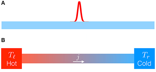
Figure 1. Schematic illustration of the (A) closed system set-up and the (B) open system set-up, commonly used to study heat transport. In (A), a localized heat pulse is introduced at some point in a system in thermal equilibrium and its subsequent time-evolution is observed. In (B), the system is attached to two heat reservoirs at different temperatures and the NESS properties, such as current and temperature profile are studied.
2.1. Signatures in the Closed System Set-Up
• Slow decay of energy current auto-correlations: A commonly followed approach for determining the N dependence of j or equivalently the thermal conductivity κ, is to use the closed system Green-Kubo (GK) formula [23, 24]:
where , with j(x, t) defined in Equation (8), is the total current in the system. The average is evaluated with initial conditions chosen from a thermal distribution and time-evolution given by the closed system dynamics. This formula relates the thermal conductivity κ to the integral of the equilibrium heat current auto-correlation function . Numerical simulations as well as several theoretical treatments find that CJ(t) in a closed system generically decays with time as a power law with 0 ≤ α ≤ 1 [2, 3, 7, 9, 12, 33, 38–51]. As an example we show in Figure 2 data from simulations [7] of the alternate mass hard particle gas, where we see a decay with α ≈ 0.33. Such a power-law time dependence implies, from Equation (10), a divergent thermal conductivity. To see the dependence on system size one heuristically puts a cutoff tN ~ N in the upper limit of the time integral, the argument being that this is the time taken by sound modes to explore the full system of size N. Performing the time integral in Equation (10) with this cut-off, one finally gets κ ~ Nα. An interesting example where this procedure fails has been pointed out in a recent work [52, 53].
• Super-diffusive spreading of initially localized energy pulse: Here one looks at the spreading of a localized energy pulse in a thermally equilibrated system. One takes an initial configuration chosen from a thermal distribution with average local energy , uniform across the system. Imagine putting an extra amount of energy ϵ0 to a few particles in a region inside the bulk to create a pulse of excess energy locally. As the system evolves according to the closed system dynamics, this localized energy perturbation starts spreading across the system. Let ϵ(x, t) represent the excess energy density (above e0) at the point x and at time t (averaged over the initial distribution). This quantity starts as a δ-function at t = 0 and then starts spreading with time. Note that ∫ dx ϵ(x, t) = ϵ0, the total injected energy is conserved under the closed system dynamics. For a diffusive system, the perturbation would evolve according to the diffusion equation ∂ϵ(x, t)/∂t = D∂2ϵ(x, t)/∂x2 and in macroscopic length-time scales, the perturbation profile at time t would be given by a Gaussian
For a system with AHT, one instead finds the following scaling form [4, 8]
with a scaling exponent 1/2 < γ < 1. The two limits γ = 1/2 and 1 correspond respectively to diffusive and ballistic transport. In Figure 3 we show results for energy pulse spreading obtained in [8] for the alternate mass hard particle gas model. The main plot shows the scaling x ~ tγ, with γ = 3/5 of the central part of the distribution. The central part of the distribution was found to fit to the Lévy function which is the propagator of Equation (4) with μ = 1/γ. The mean square deviation (MSD) defined as
with mean taken as zero, was seen to scale as , with β = 4/3, as opposed to a diffusive system with β = 1. It was also noted that the MSD width exponent, β, is related to the thermal conductivity exponent α as β = 1 + α (see section 3.1.2 for details). To compute the MSD and relate the exponents β and γ is a somewhat subtle issue and requires one to note that the scaling function is valid in the bulk region |x| ≲ t, beyond which ϵ(x, t) decays rapidly (see discussion in section (3.1.1) in the context of Lévy-walk model). From properties of the Lévy distribution one gets, in the regime tγ < < x ≲ t, the scaling form . Using these asymptotics and computing gives us the leading behavior σ2(t) ~ t3−1/γ which then leads to the relation β = 3 − 1/γ. Observations from several other numerical simulations have confirmed the super-diffusive behavior [8, 54–59].
• Super-diffusive evolution of density correlations: The anomalous signature discussed in the previous point can also be observed alternatively by looking at the spreading of the equilibrium spatio-temporal correlation function of the energy density e(x, t) defined as
where the average is taken over the equilibrium initial conditions. For diffusive systems this correlation has the Gaussian form in Equation (11), while for systems with AHT this has the scaling form in Equation (12) and one again has super-diffusive growth of the MSD [21], now defined as
This MSD can be related to defined above, using linear response theory and both have ~ tβ scaling. In the case of AHT, observing the scaling form in Equation (12) usually requires one to subtract contributions of sound modes which travel ballistically. The theory of non-linear fluctuating hydrodynamics (NFH) provides a framework in which one can systematically describe the super-diffusive scaling of the correlation [22, 47, 60–63]. This theory is based on writing hydrodynamic equations for the conserved quantities in the system which for the Hamiltonian in Equation (5) are the total energy, total momentum and the total number of particles (or volume). This framework of NFH is discussed in detail in section 3.2. A connection can be made between the super-diffusive scaling () of the energy correlations and the power-law decay, ~ tα−1, of the current-current correlations [4, 58, 59], which can be seen as follows. Starting from the continuity equation for energy, one can obtain the relation [61, 62] on the infinite line
Multiplying by x2 on both sides and integrating over all the range of x one gets
Assuming the expected forms σ2(t) ~ tβ and we get the relation α = β − 1.
2.2. Signatures in the Open System Set-Up
• Diverging thermal conductivity: As discussed above in the open system set-up, one connects the system at the two boundaries to heat reservoirs at unequal temperatures Tℓ ≠ Tr. A common model for baths is to write Langevin dynamics for the boundary particles involving dissipation and noise term satisfying the fluctuation-dissipation relation. For a chain of interacting particles described by the Hamiltonian in Equation (5) the equations of motion for the boundary particles would read
where fi = −∂H/∂qi. The noise terms ξℓ,r are Gaussian white noise terms, with zero mean and correlations . The remaining particles evolve according to Equation (6). After a long time the system reaches a non-equilibrium steady state (NESS) and we can measure the steady state current j as average of the local current j(x, t) defined through Equation (8). In the steady state this will be independent of time as well as the bond where we measure the current. One can then check if the system size N scaling of this steady state current j has the expected form j ~ Nα−1, where α < 1 for anomalous systems. Alternatively one can define the κ = jN/(Tℓ − Tr) and see how this scales with N. For a large class of non-linear interaction potentials, it has been observed that the thermal conductivity κ ~ Nα with 0 < α < 1 for large N [6, 7, 10, 11, 63, 64]. As an example, we show in Figure 4 data from [10] for the FPUT-β chain, where one finds α ≈ 0.33.
• Non-linear temperature profile: The local temperature at a site on the lattice can be defined through the relation , where the average is taken in the NESS. For diffusive systems, the temperature profile obtained would be linear for small ΔT = Tℓ − Tr, as expected from solving Fourier's law with a constant κ. It is important to note that non-linear temperature profiles can also be obtained in case of diffusive transport if the thermal conductivity κ is temperature-dependent and ΔT is large. On the other hand, for many systems with AHT, one finds a strongly non-linear temperature profile even when ΔT is made arbitrary small [5, 10, 11, 26, 34, 36, 65]. Quite often the profiles are characterized by divergent slopes at the boundaries. In Figure 5 we show the temperature profile in the FPUT-β model and one can see the characteristic non-linear nature. Note that the definition of local temperature makes sense (and is useful) only if this temperature predicts correctly other local observables, for example higher moments of the velocity. This was also verified in [10] and also shown in Figure 5. Typically one finds that the temperature difference δT(x) = |Tℓ − T(x)| scales as (δx)μ, with distance δx from the boundary, where 0 < μ ≤ 1. The exponent μ has been referred to as the meniscus exponent [66]. This exponent is non-universal in the sense that it depends on details of boundary conditions, unlike the conductivity exponent α.
• Green-Kubo-type relation for open systems: Analogous to the Green-Kubo formula in the closed system set-up given by Equation (10), an exact formula exists in the open system set-up that relates the current response to a small temperature difference ΔT = Tℓ − Tr. This is given by [67]
The time auto-correlation is computed by averaging over equilibrium initial conditions as well as the open system dynamics which includes the stochastic baths (at equal temperatures). This formula is valid for a finite size system. We note that for systems with AHT, unlike with Equation (10), in the open set-up we do not require the use of an upper cut-off tN ~ N for estimating the size dependence of conductivity. In this case the linear response current can be evaluated directly from Equation (20) for any finite system of size N and thereby one can verify the form j/ΔT ~ Nα−1. This approach has been discussed for example in [63, 64]. It was observed in [64] that, for the so-called random collision model studied by them, both and showed a t−2/3 decay at times t ≲ N. However, the exponential decay for the open case begins at tN ~ N while for the closed system (with periodic boundary conditions) this begins at . This was understood as arising from the time scale associated to the spreading of sound modes. Note that if we put the cut-off as the upper limit in the time-integral of Equation (10) then we would get the wrong conductivity exponent. In order to get the correct exponent in the closed system set-up, one has to by hand set the cut-off at tN ~ N based on consideration of the practical transport set-up which has baths at the boundaries.
Recently, in a model system of AHT the relation in Equation (3) has been established using the above formula and a heuristic approach based on fluctuating hydrodynamics [36]. An explicit expression of the kernel was obtained for a specific model, using which one can understand the divergence of κ as well as the singular features in the temperature profile. A detailed discussion of this method is given later in section 4.2.3.
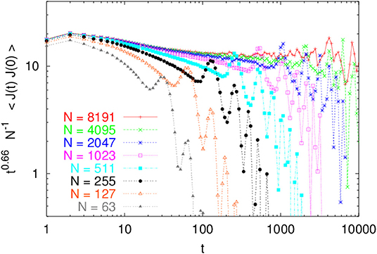
Figure 2. Total scaled heat current auto-correlation, t0.66N−1〈J(t)J(0)〉, in the alternate mass hard particle gas for mass ratio 2.2 and T = 2.0 (adapted from Grassberger et al. with permission from [7] Copyright (2002) by American Physical Society).
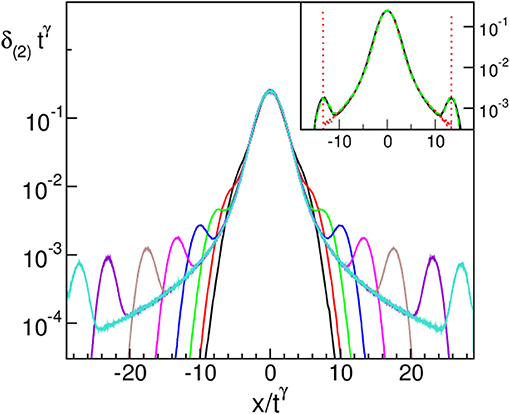
Figure 3. Scaled perturbation profiles at times t = 40, 80, 160, 320, 640, 1, 280, 2, 560, and 3, 840, with γ = 3/5. The profiles have been obtained by averaging over large number of realizations. In the inset, the profile at t = 640 (solid line) is compared with the propagators of a Lévy walk with an exponent ν = 5/3 with a fixed velocity v = 1 (dotted line) or with velocity chosen from a Gaussian distribution with mean 1 and variance 0.036 (dashed line) (adapted from Cipriani et al. with permission from [8] Copyright (2005) by American Physical Society).
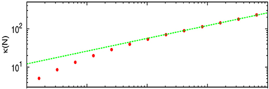
Figure 4. FPUT-β model: Results for conductivity κ vs. N for Tℓ = 2.0 and Tr = 0.5. The last five points fit to a slope of 0.333 ± 0.004 (adapted from Mai et al. with permission from [10] Copyright (2007) by American Physical Society).
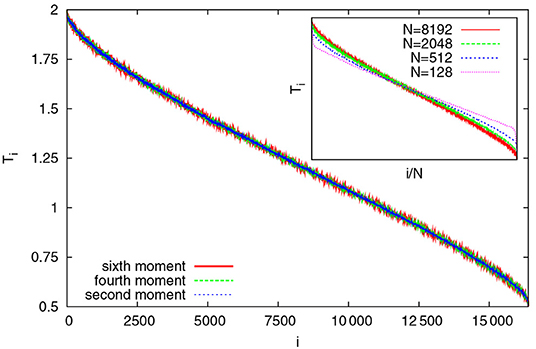
Figure 5. FPUT-β model: Kinetic temperature profile for a system with N = 16384, Tℓ = 2.0, Tr = 0.5. Assuming a Gaussian local velocity distribution, the temperatures as defined from the first three even moments are shown; their agreement vindicates the assumed Gaussian velocity distribution. (Inset) Normalized temperature profiles for different N (adapted from Mai et al. with permission from [10] Copyright (2007) by American Physical Society).
3. Phenomenological Approaches for Anomalous Heat Transport
In this section we will discuss two different approaches that have tried to understand the various aspects of AHT mentioned above. The first is a completely heuristic approach where one assumes that the heat carriers perform Lévy walks instead of random walk which is expected for diffusive heat transfer. This method has been used to explain spreading of localized energy pulses, steady state properties and current fluctuations [8, 39, 57, 66, 68–71]. The second approach is a microscopic one where one starts by writing hydrodynamic equations for the conserved quantities of the Hamiltonian dynamics. One then phenomenologically adds noise and dissipation terms satisfying fluctuation dissipation relations and this allows one to study equilibrium fluctuations in the system. In particular, using the formalism of fluctuating hydrodynamics, one can compute dynamical correlation functions which contain information on AHT.
3.1. Lévy Walk Description of Anomalous Heat Transport
3.1.1. Lévy Walk Description in the Closed Set-Up
In this description one thinks of energy as being carried by Lévy walkers, each of which carry a fixed amount of energy. It follows that the local energy density and energy current at any point can be taken to be directly proportional to, respectively, the particle density and current. Let us also assume that the local temperature is proportional to the local energy density and hence to the density of particles.
Definition of the Lévy walk [72–74]: At each step of the walk, a particle chooses a time of flight τ from a specified distribution, ϕ(τ), and then moves a distance x = cτ at a fixed speed c, with equal probability in either direction. More generally one can consider the velocity c to be drawn from a distribution. Let P(x, t)dx denote the probability that the particle is in the interval (x, x + dx) at time t. Note that P(x, t) also includes events where the particle is crossing the interval (x, x + dx), in addition to the events in which the particle lands in the interval at time t. If a particle starts at the origin at time t = 0, the probability P(x, t) satisfies
where is the probability of choosing a time of flight ≥ τ. Here we consider Lévy walkers with a time-of-flight distribution
which decays, at large times, like a power law ϕ(t) ≃ A t−ν−1 with . For this range of ν the mean flight time is finite but 〈t2〉 = ∞.
Some properties of the Lévy walk: Taking the Fourier Laplace transform we get
where and .
For asymptotic properties it is useful to find the form of for small k, s. The Laplace transform is given by:
and Γ(u) is the Gamma-function. Hence we get:
where d = bA/(2〈t〉). Taking the inverse Fourier-Laplace transform of this gives us the propagator of the Lévy walk on the infinite line. This corresponds to a pulse whose central region is a Lévy-stable distribution with a scaling x ~ t1/ν. This can be seen by expanding Equation (25) for ck/s < < 1 to get . The difference with the Lévy-stable distribution is that the Lévy-walk propagator has ballistic peaks of magnitude t1−ν at x = ±ct and vanishes outside this. The overall behavior of the propagator is as follows [72]:
The time evolution of the Lévy-walk propagator, obtained from direct simulations of the Lévy walk, is shown in Figure 6. We also plot the Lévy-stable distribution obtained by taking the Fourier transform of P(k, t) = e−c cos(νπ/2)|k|νt.
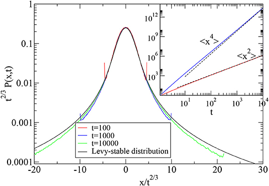
Figure 6. Plot of the scaled distribution t2/3P(x, t) vs. x/t2/3 of the Lévy walk on the open line for ν = 3/2 at three different times. Also shown is a plot of the Lévy-stable distribution. The inset shows a plot of the mean square displacement and the fourth moment and a comparison with the exact asymptotic forms (dashed lines) given by Equations (27, 28). In all plots the time to and c are set to one.
Various moments of the distribution can be found using the relation , or its Laplace transform given by . Using Equation (25) we get in particular the following leading behavior
We see that for 1 < ν < 2 the motion is super-diffusive [73, 74]. The most interesting characteristics to note about the Lévy walk are the fact that the probability distribution has finite support (|x| ≤ ct), in the bulk it coincides with the Lévy distribution with scaling x ~ t1/ν and finally the mean square displacement (MSD) 〈x2〉 ~ tβ with β = 3 − ν. Note that the usual Lévy stable distribution has a diverging second moment, however the Lévy walk has a finite MSD and this follows from the finite support |x| ≤ ct of the corresponding distribution. Indeed, on using this cutoff and the power-law form of the Lévy near the cut-off (see Equation 26) gives us the expected scaling exponent β = 3 − ν.
Lévy walks and AHT: The first proposal suggesting the Lévy walk model to describe anomalous heat transport was made in [68]. This idea was tested for a microscopic model in [8] where it was shown that the spreading of a heat pulse in a thermally prepared alternate mass hard particle gas was super-diffusive and is well-described by the Lévy walk model. In Figure 3 we show the evolution of a localized perturbation. The main plot shows the x ~ t3/5 scaling of the central part of the distribution while the inset shows a fit to the expected Lévy distribution (for a LW with ν = 5/3) with a single fitting parameter. It was also shown that the MSD of the energy has the scaling ~ t4/3 as expected from the relation β = 3 − ν for LW. Finally it was proposed using linear response ideas that the exponent β and the conductivity exponent α should be related as α = β − 1 which gives α = 1/3 for the present system. This agrees with known results for the alternate mass hard particle gas. The validity of the Lévy walk description of pulse propagation was further verified in [39] for a hard particle gas interacting via a square well-potential and in [57] for the FPUT chain. All these cases were described by the same Lévy-walk exponent ν = 5/3.
3.1.2. Lévy Walk Description of the Open Set-Up
We now discuss the case of the open system consisting of a finite segment (0, L) that is connected to two reservoirs at the ends. The use of the Lévy walk model to study NESS properties in AHT was first proposed in Lepri and Politi [66] where the authors considered a finite lattice of N sites containing a collection of Lévy walkers. The system was connected at it's two ends to infinite reservoirs that contained sources emitting Lévy walkers at fixed constant rates. A Lévy walker crosses from the reservoir into system with probability one, but while exiting from system into reservoir, it can get reflected with probability R. A particle exiting the reservoir is eliminated. The authors in Lepri and Politi [66] considered a discrete version and studied this problem numerically. The strategy was to write appropriate master equations for the probability evolution and obtain the steady state solution numerically. One of the main observations in the paper was that the NESS profile for P(x) was non-linear and was singular at the boundaries. In Figure 7A we show a plot of the profile for the case R = −0.1, compared with simulation results for the temperature profile in the momentum exchange model (HCME), with free BC and a specific choice of exchange rate. One sees very good agreement. As noted in section 2.2 in the context of temperature profiles in systems with AHT, one can define a “meniscus” exponent, μ, through the observed scaling form P(x) ~ (δx)μ for small distances δx from any boundary. Based on their numerical observations (see Figure 7B) the authors in [66] conjecture the relation
It was noted in [66] that the value R = −0.1 was unphysical but made mathematical sense in the master equation (see [66] for further discussions on this point) and gave the best agreement with the momentum exchange simulation profile.
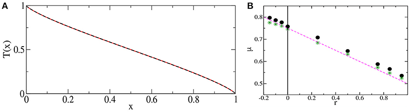
Figure 7. (A) Temperature profile of the oscillator chain with conservative noise with free boundary condition and λ = γ = 1 (solid line) and solution of the master equation with reflection coefficient R = −0.1 (dashed line) (reprinted from Lepri and Politi [66]). (B) Dependence of the meniscus exponent μ on the reflection probability r for ν = 3/2. Note that r in this figure is denoted by R in this review. Full circles and stars are measures from fitting of P(x) and Q(x), respectively (see text). The dashed line is given by formula (29) (adapted from Lepri and Politi with permission from [66] Copyright (2011) by American Physical Society).
Some exact results were obtained for the Lévy walk model with particle reservoirs, for the special case of perfectly transmitting boundary walls (i.e., R = 0) [69] which we now describe. We note that for the Lévy walker, at any given time, a particle could either be passing over a point x or could have landed precisely at the point. Hence, in addition to the probability density P(x, t), it is convenient to define the probability Q(x, t)dxdt that a particle lands precisely between x to x + dx in the time interval (t, t + dt). We now specify the boundary conditions required to set up a non-equilibrium current carrying steady state. For this, we consider the region x ≤ 0 as the left reservoir with Q(x, t) = Ql for all points in this region. Similarly, we set Q(x, t) = Qr in the region x ≥ L corresponding to the right reservoir. In the steady state, the distributions become time-independent and Q(x, t) = Q(x), P(x, t) = P(x) satisfy [69]
where and as mentioned earlier after Equation (21). The terms on the right hand side of the above equation for Q(x) represent different contributions. The first term represents the contributions from walkers that start from various points y and land at x. The second and the third term represent contributions from walkers starting, respectively, from left and right reservoirs and landing at x. Similarly, the terms on the right hand side of Equation (31) for P(x) can also be interpreted in the same way except now, events in which the walkers are passing over x, in addition to the events in which they land at x at a given time, also contribute.
Interestingly, it turns out that the problem of finding Q(x) can be related to the problem of the escape probability [75] of a Lévy walker on the interval (0, L). Let H(x) denote the probability with which a Lévy walker, starting at position x, arrives at the left reservoir (region x < 0) before arriving at the right reservoir (region x > L). It can be shown that H(x) satisfies [69]
The probability Q(x) can now be expressed in terms of H(x) as Q(x) = (Ql − Qr)H(x) + Qr, which can be checked easily to satisfy Equation (30).
If one considers a Lévy flight with distribution ρ(z) = [ϕ(z/c) + ϕ(−z/c]/(2c) of steps z, the probability H(x) that starting at x, the flight hits first the left bath satisfies exactly Equation (32). Hence by following the same mathematical steps as in [75] to study equations, such as (30) or (32), one can show that, in the large L limit, the solution Q(x) of (30) [and H(x) of (32)] satisfies
with Q(0) = Ql and Q(L) = Qr [and H(0) = 1 and H(1) = 0 for (32)] with a solution of (33), for a ϕ(τ) decaying as in (22), which satisfies
We can integrate this equation to get Q(x), with the integration constant and B being then determined from the boundary conditions Q(0) = Ql and Q(L) = Qr. One finally obtains
and 2F1(a, b, c, z) is the hypergeometric function. For large L, the right hand side of Equation (31) is dominated by the range |y−x| ≪ L and therefore
The exact results of Equations (34) have been verified in [69] from direct numerical solution of Equations (30, 31) and it was noted that the density profiles were similar to the temperature profiles seen in AHT.
Next we discuss the steady state current j(x) which is given by
This can be seen to be the difference between the flow from left to right and from right to left. The contribution from 0 < y < ∞ to the integral corresponds to particles crossing the point x from left to right which is obtained by multiplying the density of particles at x − y with the probability ψ(y/c) that they have a flight time larger than y/c. The contribution from −∞ < y < 0 to the integral corresponds to a similar right-to-left current. After performing a partial integration and using the boundary conditions Q(0) = Ql and Q(L) = Qr, one obtains
Using Equation (33) it is easy to see that dj/dx = 0 which implies that the current in the steady state is independent of x, as expected. Hence, evaluating the current at x = 0 and using Equation (34), we get for large L
From Equation (27) we then get the relation α = β − 1, between the conductivity exponent of AHT and the MSD exponent for Lévy-walk diffusion. This relation for Lévy diffusion was pointed out in [68] and verified in simulations in 1D heat conduction models [8, 21]. A derivation based on linear response theory has been given in [59]. Finite size corrections to the results in Equations (34, 39) were recently obtained in [76].
In the large L limit by using Equation (36) in Equation (38) we obtain
Above equation is the analog of Fourier's law Equation (1) with the important difference that in the linear response regime the current at a point gets contributions from the temperature gradients at other parts of the system as well.
The above treatment can be generalized for arbitrary values of the reflection probability R [37] and this leads to the following general non-local form of the current
Remarkably we note that for ν = 3/2 (α = 2 − ν = 1/2), the expression above is identical to the expression for with v = x/L, v′ = y/L, given later in Equation (112).
3.2. Non-linear Fluctuating Hydrodynamics Description of Anomalous Heat Transport
We now discuss a completely different approach for understanding AHT. In this approach the starting point is the Hamiltonian dynamics of the system. The idea is to consider the effective dynamics of the slow conserved fields using some coarse graining. One finds that the evolution of small fluctuations around equilibrium can be described by fluctuating hydrodynamics. Solving these equations using mode coupling theory, detailed predictions can be made on the form of equilibrium spatio-temporal correlation functions of the conserved fields. In particular, we will see that it predicts the super-diffusive spreading of energy perturbations with Lévy-law scaling, and the slow decay of energy current auto-correlation functions. We will here describe the theory for generic anharmonic systems with three conserved quantities, namely volume, momentum, energy [61], and present some numerical results which verify the predictions of the theory.
Let us consider N particles of unit masses with positions and momenta denoted by {q(ℓ), p(ℓ)}, for ℓ = 1, …, N. The particles move on a ring of size L so that we have the boundary conditions q(N + 1) = q(1) + L and p(N + 1) = p(1). The Hamiltonian is taken to be
where we have defined the stretch variables r(ℓ) = q(ℓ + 1) − q(ℓ). It is easy to see from the Hamiltonian equations of motion that stretch r(ℓ), momentum p(ℓ), and energy ϵ(ℓ) are locally conserved and hence satisfy corresponding continuity equations. In the continuum limit, these equations take the form
where the label index ℓ has been denoted by the corresponding continuous variable x and P(x) = −V′(x) is the local force. Assume that the system starts in a state of thermal equilibrium at zero total average momentum characterized by the temperature (T = β−1) and pressure (P), which fix the the average energy and average stretch of the chain. The distribution corresponding to this ensemble is
Since the fields r(x, t), p(x, t), and e(x, t) satisfy continuity equations, they evolve slowly suggesting a slowly evolving local equilibrium picture. We consider small fluctuations of the conserved quantities about their equilibrium values, u1(x, t) = r(x, t) − 〈r〉eq, u2(x, t) = p(x, t), and u3(x, t) = ϵ(x, t) − 〈ϵ〉eq. Inserting these into Equation (44) one obtains ∂tuα = −∂xjα, where jα are the corresponding Euler currents which are functions of uαs. Expanding these currents to second order in the fields as , and then adding dissipation and noise terms (to ensure thermal equilibration) one arrives at the following noisy hydrodynamic equations
where repeated indices are summed over. The noise and the dissipation matrices, , are related to each other by the fluctuation-dissipation relation , where the matrix C corresponds to equilibrium correlations and its elements are Cαβ(x) = 〈uα(x, 0)uβ(0, 0)〉.
It is useful to define normal modes of the linearized equations (dropping u2 terms in Equation 46) through the transformation , where the matrix R acts only on the component index and diagonalizes A, i.e. RAR−1 = diag(−c, 0, c). The diagonal form implies that there are two sound modes, ϕ±, traveling at speed c in opposite directions and one stationary but decaying heat mode, ϕ0. The quantities of interest are the equilibrium spatio-temporal correlation functions , where s, s′ = −, 0, +. Because the modes separate linearly in time, one argues that at large times the off-diagonal matrix elements of the correlator are small compared to the diagonal ones and that the dynamics of the diagonal terms decouples into three single component equations. After including the non-linearity it is seen that to leading order the equations for sound modes have self-coupling terms of the form . These then have the structure of the noisy Burgers equation, for which the exact scaling function, denoted by fKPZ, are known. For the heat peak the self-coupling coefficient vanishes for any interaction potential. Thus, one has to study the sub-leading corrections, and calculations using the mode-coupling approximation result in the symmetric Lévy walk distribution, with a cut-off at x = ct. While this is an approximation, it seems to be very accurate. For the generic case of non-zero pressure, i.e. P ≠ 0, which corresponds either to asymmetric inter-particle potentials or to an externally applied stress, the prediction for the left moving, resp. right moving, sound peaks, and the heat mode are
where fKPZ(x) is the KPZ scaling function discussed in [61, 77], and tabulated in [78]. The scaling function is given by the Fourier transform of the Lévy characteristic function e−|k|ν, with a cut-off at x = ct. The scaling parameters λs and λe are known explicitly. On the other hand for an even potential at zero pressure, i.e., P = 0, all self-coupling coefficients vanish. As a result the scaling solutions within mode-coupling approximation change and one obtains
where fG(x) is the unit Gaussian with zero mean. The scaling parameters is not known from microscopics while is known explicitly in terms of .
Here we present molecular dynamics simulation results for the FPUT chain that were obtained in [63] which verify the predictions of NFH. In Figure 8, top panel, the two-point correlation functions C00(x, t), C++(x, t) and C−−(x, t) are plotted as a function of x for three values of time t = 800, 2, 400 and 3, 200. The parameters used in this plot are k2 = 1.0, k3 = 2.0, k4 = 1.0, T = 5.0, P = 1.0 for which one gets c = 1.80293 and we also see there is a good separation of the heat and sound modes. In Figure 8, bottom panel we also find an excellent collapse of the heat mode and the sound mode data with the expected scalings. The scaled data for the heat mode fits very well to the Lévy-scaling function whereas the same for the sound-mode still shows some asymmetry but is quite close to the KPZ function. The numerically estimated values of the constants λs,e are λs = 0.46 and λe = 5.86. These are in close agreement to the theoretically obtained values λs = 0.396 and λe = 5.89.
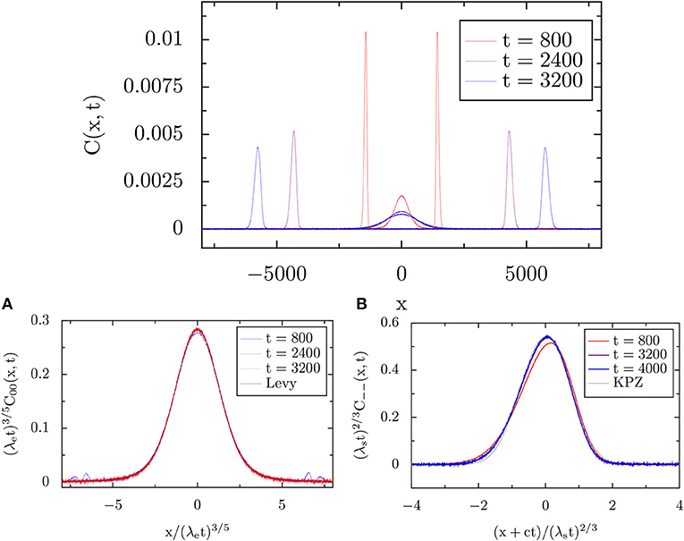
Figure 8. (Top) Plots of the heat mode correlation C00(x, t) (central peaks) and the sound mode correlations C++(x, t) and C−−(x, t) (right and left moving peaks) in the FPUT chain, at three different times, for the parameter set with k2 = 1.0, k3 = 2.0, k4 = 1.0, T = 5.0, P = 1.0, and system size 16, 384. The speed of sound was c = 1.80293. We see that the heat and sound modes are well-separated. The numerical data in this plot were obtained by averaging over around 106 − 107 initial conditions. (Bottom) The heat mode (A) and the left moving sound mode (B) correlations, respectively, C00(x, t) by C−−(x, t) are plotted at different times, using a Lévy-type-scaling for the heat mode and KPZ-type scaling for the sound mode. Here we observe a very good collapse of the data at different times. Moreover, we observe a good fit to the Lévy-stable distribution with λe = 5.86 and a reasonable fit to the KPZ scaling function, with λs = 0.46. The parameters used in this plot are k2 = 1.0, k3 = 2.0, k4 = 1.0, T = 5.0, P = 1.0 (adapted from Das et al. with permission from [63] Copyright (2014) by American Physical Society).
4. Stochastic Models: Exact Results on Fractional Equation Description
It is now well-understood that conservation laws play an important role in observation of super-diffusive transport in one-dimensional systems. As we saw in the previous section, NFH provides some understanding of the emergence of Lévy-walk behavior, which seems to capture several aspects of anomalous transport. However, providing a completely rigorous microscopic derivation of the Lévy-walk picture in a Hamiltonian model has been difficult, though there have been some attempts [79]. While generic non-linear Hamiltonian models are difficult to analyze, analytical results have been obtained for harmonic chains whose Hamiltonian dynamics is perturbed by stochastic noise that breaks integrability of the system [9, 30, 52]. These stochastic models attempt to mimic non-linear chains and for these models, several exact results both in the closed system set-up and the open system set-up have been obtained. In particular one can rigorously establish non-local response relation Equation (3) and the fractional diffusion equation Equation (4). There are two widely studied stochastic models which we discuss below.
4.1. Harmonic Chain With Volume Exchange
This model is defined on a one dimensional lattice where each site carries a “stretch” variable ηi, i ∈ ℤ and the energy of the system is . The dynamics has two parts: (a) a deterministic part given by and (b) a stochastic exchange part where ηs from any two randomly chosen neighboring sites, are exchanged at a constant rate γ. We refer to this model as Harmonic chain with volume exchange (HCVE). This model was introduced in [30] where it was shown that the energy current auto-correlation decays as , implying super-diffusive transport. It is easy to see that this system has only two conserved quantities namely, the total “volume” and the total energy . The evolution of the density fields corresponding to these conserved quantities at the macroscopic length and time scales was studied in [62] using NFH, where it has been shown that this model has two normal modes - one diffusive sound mode and a -asymmetric Lévy heat mode. Subsequently, it was rigorously shown that the local energy density e(x, t) satisfies a (3/4)-skew-fractional Equation [31]
with Δ as the usual Laplacian operator. In the Fourier domain, defined by , the above equation reads as
Note that for the diffusive case the analog of the above equation would be . The above results suggest that, in the open set-up where the system is connected to two reservoirs at different temperatures, this model would exhibit anomalous scaling of the steady state current j with system size N. In [30], it has been numerically shown that indeed . Recently, an understanding of the open system was achieved using the fractional equation description, which we now discuss [34]. An aspect that we will point out here is that the fractional-equation-type description in the open-set up is strongly dependent on boundary conditions (fixed or free or mixed).
For the open system case, we consider a finite lattice of size N, connected to two thermal reservoirs at temperatures Tℓ and Tr on the left and right boundaries. The dynamics of the ηi, i = 1, 2, …, N now gets modified to
The Langevin terms at the boundaries i = 1 and i = N appear due to the baths and ξℓ,r(t) are independent Gaussian white noises with mean zero and unit variance. We consider fixed boundary conditions η0 = ηN+1 = 0.
Our main interest is to obtain an equation in this finite system, analogous to Equation (51), to describe the evolution equation of the temperature profile. To do this we first define the local temperature and the off-diagonal correlations Ci,j(t) = 〈ηi(t)ηj(t)〉, i ≠ j, which characterize the non-equilibrium state of the system. Interestingly, it turns out that the equations for two point correlations do not depend on higher order correlations and this property leads to the model's solvability. The evolution of these quantities in the bulk (2 < i, j < N − 1) can be obtained from Equation (53) as:
The equations involving the boundary terms are given in Priyanka et al. [34]. Note that in an infinite system, we get the same set of equations with i, j ∈ ℤ. For the finite open system, solving the above equations exactly seems to be difficult. However, it was observed numerically [34] that for large N the temperature field Ti(t) scales as and the correlation field Ci,j(t) scales as Inserting these into (54), and expanding in powers of , we find at leading order the following equations
where the scaling variables are defined over {0 ≤ u ≤ ∞; 0 ≤ v ≤ 1;0 ≤ τ ≤ ∞}.
Note that for the isolated infinite system, one can follow the same procedure as above, but now replacing the scale parameter 1/N → a where a is the lattice spacing, to obtain the same set of Equations (55–57) with a different domain {−∞ ≤ u ≤ ∞; −∞ ≤ v ≤ ∞}. These equations can be solved by Fourier transforms to get a skew fractional evolution equation for of the same form as Equation (52). Defining Fourier transforms and in the variable v, we get
Solving the first Equation (58), with the condition that correlations vanish at u = ± ∞, we get
The Equation (59) relates the constant Ak to :
Using Equations (61, 62) in Equation (60) we get the infinite line equation in Equation (52).
We now go back to the open system case where the solution is more non-trivial. To solve these equations in the open set-up, we proceed as for the regular diffusive heat equation, and write the solution as sum of a steady state part and a relaxation part
where we have defined z = 1 − v. We note that under this transformation, the “anti-diffusion” Equation (55), becomes a diffusion equation, with v as the time variable and z the space variable. The relaxation part satisfies the equations given in Equations (55, 56, 57), while the steady state part satisfies these equations but with . The boundary conditions for the steady state part are given by Priyanka et al. [34]
where we have used Equation (57) to identify as the NESS current which gets determined by the boundary conditions for . In terms of the original unscaled variables, the true current is given by . The solution of the steady state equations is given by Priyanka et al. [34]
In Figure 9A, we show a comparison of the above result for steady state temperature profile with those obtained from direct simulations of the microscopic model, and we see very good agreement. It is interesting to note that the temperature profile is non-symmetric under space reversal as the microscopic model itself does not have such symmetry. This fact is also reflected in hydrodynamics where this shows in the existence of a single sound mode.
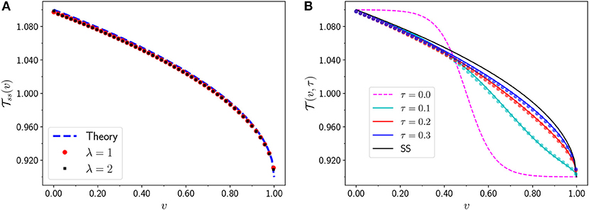
Figure 9. (A) Steady state temperature of HCVE model () as given by Equation (66) (blue dashed line) is compared with numerical simulations for parameters ω = γ = 1, Tℓ = 1.1, Tr = 0.9, and N = 1, 024, and for two different choice of λ. (B) Numerical verification of the evolution of the temperature profiles given by Equation (71) (solid lines), starting from a non-stationary profile (dashed line). The points indicate simulation results for parameters are λ = γ = 1, Tℓ = 1.1, Tr = 0.9 and N = 2, 048 (adapted from Kundu et al. with permission from [34] Copyright (2018) by American Physical Society).
For the relaxation part we look for solutions which satisfy the initial condition , and boundary conditions , . The solution of the “anti-diffusion” Equation (55), with z as time variable, with the boundary condition (56) can be obtained as [34]
Using this in (56) then gives finally the evolution equation for the temperature field
inside the domain 0 ≤ z ≤ 1. This is a non-local equation which can be recognized as a continuity equation where the current j is precisely in the form stated in Equation (3). This is the open-system analog of Equation (51). For the infinite system, a similar computation leads to Equation (68) but with the lower limit of integration replaced by z = −∞, and by taking Fourier transforms, this can be shown to reduce to Equation (52).
We now proceed to solve Equation (68) to find the temperature evolution. It is natural to expand the temperature profile in a basis set satisfying Dirichlet boundary conditions, and we choose the set . Substituting in Equation (68), we get
Further we expand the function where . Using orthogonality, we get
where and the column vector has elements . The above equation is an infinite-dimensional matrix representation of the non-local Equation (68). To solve this, we diagonalize the matrix v as ℝ−1vℝ = μ, which gives the time dependent solution as where ℝn,l = 〈αn|ψl〉 denotes the n-th element of the l-th right-eigenvector of the matrix v and the diagonal matrix μ contains the corresponding eigenvalue μl. The matrix v is real but non-symmetric and it has left eigenvectors 〈χl| whose elements are given by . The formal solution for the temperature field can then be written as
where and . Finding the eigenspectrum of the matrix v is a difficult problem as the matrix is infinite-dimensional and non-symmetric. However, one can truncate the matrix at some order and diagonalize it numerically, assuming that the spectrum converges with increasing truncation order. In [34] the authors used this approach to compute the eigenspectrum and thereby study the time evolution of the temperature profile. This is shown in Figure 9B. The spectrum is shown in Figure 10 where it is seen that for large n, which is similar to the spectrum of the non-local operator v in Equation (52) describing the evolution in infinite system. In Figure 11 we show the left and right eigenvectors and , respectively, corresponding to the first eight eigenvalues. One observes that the eigenvectors corresponding to the first four eigenvalues are real whereas the eigenvectors corresponding to the eigenvalues with n > 4 are complex and come in conjugate pairs.
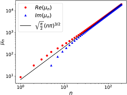
Figure 10. The real and imaginary part of the alternate eigenvalues for the matrix v in Equation (70). The first 4 eigenvalues are completely real and distinct. The higher eigenvalue comes in complex conjugate pairs. For large . For smaller n, there is a deviation from asymptotic scaling due to finite definition of the operator (adapted from Kundu et al. with permission from [34] Copyright (2018) by American Physical Society).
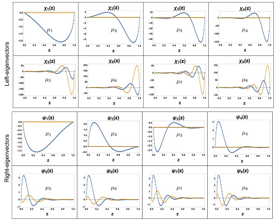
Figure 11. Left and right eigenvectors of matrix v in Equation (70) for n = 1, 2, 3, 4, 5, 6, 7, 8. The real parts are indicated by blue lines while orange denotes the imaginary part. Note that the eigenvectors corresponding to the real eigenvalues (n = 1, 2, 3, 4) are also real where the eigenvectors corresponding to complex eigenvalues (n = 5, 6, 7, 8…) are complex (adapted from Kundu et al. with permission from [34] Copyright (2018) by American Physical Society).
4.2. Harmonic Chain With Momentum Exchange
In the previous section we discussed transport in the HCVE model which has two conserved quantities, namely volume and energy. In this section, we discuss heat transport in the harmonic chain momentum exchange (HCME) model which has three conserved quantities, namely volume, momentum and energy, that are the same as the ones in usual anharmonic chains with Hamiltonian dynamics [3, 4]. The model consists of a harmonic chain of particles each of unit mass and described by the degrees of freedom qi, pi, with i ∈ ℤ, corresponding respectively to position and momentum. As for the HCVE system, the dynamics of the HCME model also has two parts: (i) the usual deterministic part given by the Hamiltonian equations , where ω is the strength of the harmonic interaction and (ii) a stochastic part consisting of exchanges of momenta between neighboring particles (chosen at random) occurring with rate γ. In the absence of the stochastic exchange, the underlying Hamiltonian dynamics is integrable and the transport in this system is ballistic due to the absence of any scattering mechanism. The stochastic exchange introduces a momentum conserving scattering mechanism, which should make the transport behavior non-ballistic. However, it turns out that the stochastic mixing is not sufficient to make the transport behavior diffusive. It has been shown rigorously that the energy current correlation in equilibrium of an infinite chain decays as t−1/2 similar to that in the HCVE model [9]. This, through the closed system GK formula in Equation (10), implies the anomalous system size scaling of the steady state current as j ~ N−1/2.
The HCME dynamics conserves the following three quantities: (a) total stretch where ri = qi+1 − qi, (b) total momentum and (c) the total energy with . As a consequence, the corresponding local densities evolve slowly in the macroscopic length and time scales. In [29], it has been analytically shown that the local energy density e(x, t) in the isolated system evolves according to the following fractional diffusion equation
and the fractional operator in Fourier space is represented by (−Δ)3/4 eikx = |k|3/2 eikx. The NESS of this system was analyzed in detail in [26–28] where the scaling j ~ N−1/2 and a closed form for the non-linear temperature profile were established. More recently the fractional-equation-type description of this system in the open set-up was further discussed in [37]. We summarize below some of these results for the open system. We first discuss the steady state and relaxation properties which is followed by the discussion on the evolution of the fluctuations and in the end we discuss the role of boundary conditions.
4.2.1. Typical Behavior of Temperature, Current, and Other Correlations
In the open system HCME set-up, the two ends are attached to two reservoirs at temperatures Tℓ and Tr. The equations of motion are now modified by adding Langevin forces to the 1st and the Nth particles:
for i = 1, 2…, N, where ξ1,N are independent Gaussian white noises with mean zero and unit variance, λ is the friction coefficient, and the parameter ζ has been introduced to describe different boundary conditions. Free boundary conditions correspond to ζ = 1 while fixed boundary conditions are given by ζ = 2. We will first discuss the fixed boundary case, i.e., ζ = 2.
We will be interested not only in NESS properties, such as the form of the temperature profile and the current scaling with system size but also in the temporal evolution of the temperature from some arbitrary initial profile to the steady state form. As in the case of the HCVE model, the analytical tractability of the HCME system comes from the fact that the evolution of the two-point correlations is given by a closed set of equations. The two point correlations include Ui,j = 〈qiqj〉, Vi,j = 〈pipj〉, and Zi,j = 〈qipj〉 and the local temperature defined as consists of the diagonal elements of V. For these, one obtains a set of coupled linear equations, similar in form to Equation (54), which one needs to solve with appropriate boundary and initial conditions. The number of equations in this case is much larger than the HCVE case and hence it is even more difficult to solve them analytically for finite N. Observations from numerical solutions of these equations reveal [27] that for large N, the temperature field Ti and the correlations show the following scaling behaviors: and . Hence, for large N it is instructive to construct solutions of these scaling forms. Inserting these scaling forms in the discrete equations of the two point correlations and taking the large N limit one finds, at leading order in , the following partial differential equations [27]
where the scaling variables are defined over the domain u ∈ [0, ∞) and v ∈ [0, 1] with boundary conditions and T(0, τ) = Tℓ and T(1, τ) = Tr. We again note that for the isolated infinite system, one can follow the same procedure as above, but now replacing the scale parameter 1/N → a where a is the lattice spacing, to obtain the same set of Equations (74–76) with a different domain {−∞ ≤ u ≤ ∞; −∞ ≤ v ≤ ∞}. Defining Fourier transforms and in the variable v, we get
Solving the first Equation (77), with the condition that correlations vanish at u = ±∞, and requiring that is real [since ], we get
The Equation (78) relates the constant Ak to :
Using Equations (80, 81) in Equation (79) we get
which is the Fourier representation of Equation (72), with .
We now go back to the open system case where the solution is more non-trivial. The boundary conditions for this case are given by and T(0, τ) = Tℓ and T(1, τ) = Tr (see [27, 37]). Note that the domain of the v variable in [27] is v ∈ (−1, 1).
In the steady state, the analytical solutions of these equations [with ∂τT(v, τ) = 0] were obtained in [26] and are given by
where , ΔT = Tℓ − Tr and for n ≥ 0. From Equation (76) we see that the current is given by
Note that both the temperature profile and the current are independent of the friction coefficient λ. This is true only for the special case of fixed boundary conditions. Note also that the temperature profile in the steady state is intrinsically non-linear as can be seen in Figure 12A where one observes excellent agreement with data from simulations of the microscopic dynamics in Equation (73). It can be shown that the temperature profile at both boundaries scales as ~ (δv)μ with μ = 1/2 where δv is the distance from the boundary [26]. This singular behavior of Tss(v) is a common signature of anomalous transport and it is characterized by the meniscus exponent μ. The value of μ however is non-universal and depends strongly on the boundary conditions. We will discuss this in section 4.2.3.
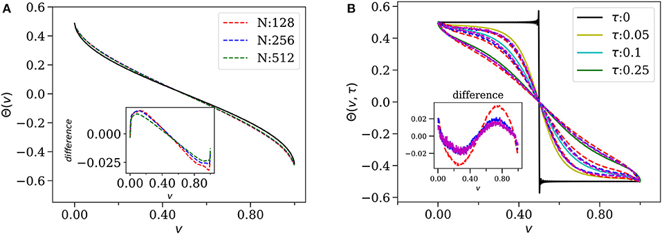
Figure 12. (A) Comparison of temperature profiles obtained theoretically from Equation (83) (solid black line) with the same obtained from direct numerical simulations of microscopic system for N = 128, 256, 512. The agreement between theory and numerics becomes better for larger N as can be seen in the inset where the difference between theoretical curve (Equation 83) and simulation data are plotted for various system sizes. (B) Time evolution of temperature starting from an initial step profile. The function , with given by Equation (93), is plotted and compared with direct numerical simulations. The dashed lines indicate simulation results for the time-evolution in HCME at different scaled times (τ), for system sizes N = 128 (red), N = 256 (blue), N = 512 (magenta), while the solid lines are obtained from the theory. The boundary temperatures were fixed at Tℓ = 1.5 and Tr = 0.5 (adapted from Kundu et al. with permission from [37] Copyright SISSA Medialab Srl, IOP Publishing).
To solve for the approach toward the above steady state results, we proceed as for the HCVE model. Separating the relaxation part and the steady state part we write
Since the relaxation parts satisfy Dirichlet boundary conditions and , we expand them in the Dirichlet basis for n = 1, 2, 3, … as
After inserting these expansions in Equations (74–76) and using the orthogonality property of the αn(v) functions, one gets the following (infinite order) matrix equation for the evolution of the components :
with , Λnl = λnδnl is a diagonal matrix with and the constant . In the position basis, the above equation can be written as
where the operator p is represented as
From this representation one can identify the action of p on the set of basis functions ϕm (which satisfy Neumann boundary conditions) [4, 37].
For the time evolution we need the eigenspectrum of p with Dirichlet boundary conditions. The eigenstates ψn(y) and eigenvalues μn can be obtained by diagonalizing the matrix in Equation (90). In [27] the spectrum was obtained numerically by diagonalizing truncated form of the infinite-dimensional matrix p. An alternate method was recently proposed in [37] which gives the spectrum directly as roots of a transcendental equation and explicit series form expressions for the wave functions in the ϕn basis. The numerical values of the computed eigenvalues are plotted in Figure 13A, where we see that for large n the eigenvalues scale as . At smaller values n there is a systematic deviation from the Neumann spectrum, λn, for example the first three eigenvalues (μn) are given by μ1 ≈ 2.75, μ2 ≈ 12.02, μ3 ≈ 24.22. As shown in the inset of Figure 13A the relative difference between μn and λn decreases as 1/n. The first few numerically computed eigenvectors are shown in Figure 13B where they are compared with the basis functions αn which are the Dirichlet eigenfunctions of the usual Laplacian. We observe that they are different and in particular show a non-analytic behavior at the boundaries. For example near the boundaries one finds , where δv is the distance from the boundaries. The eigenspectrum of fractional operator in a bounded domain, with different boundary conditions, has been discussed earlier in the literature, using somewhat heuristic approaches [75, 80–82]. However, their connection to the spectrum of p defined here is unclear.
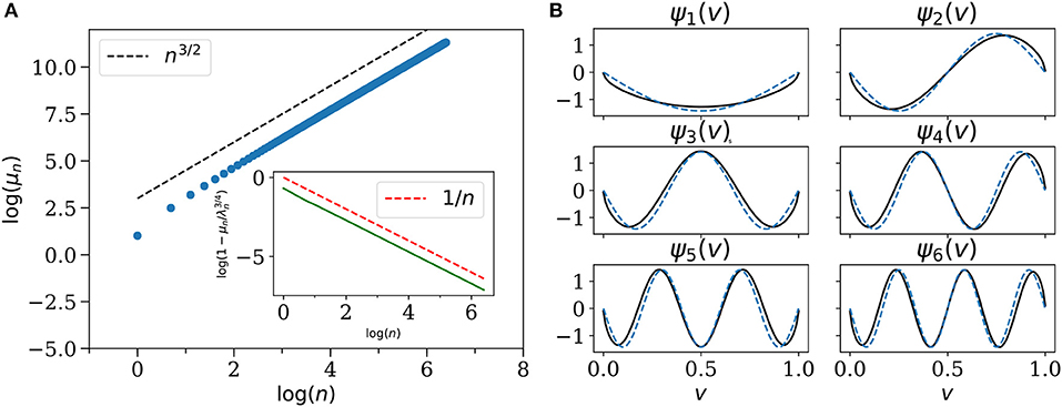
Figure 13. (A) Eigenvalues of the fractional operator in Equation (90) corresponding to Dirichlet boundary conditions. For large n, the slope is seen to approach that of n3/2 (black dashed line). For small n there is a systematic difference between the Dirichlet and Neumann eigenvalue and the inset plots the difference between the two. For large n the difference between the two decreases inversely with n. (B) The first six eigenvectors, ψn(v) (black lines), are compared to the corresponding Dirichlet eigenfunctions of Laplacian, i.e., sin-functions (blue dashed lines). The eigenstates are different from sin-functions, especially near the boundaries, even for large n (adapted from Kundu et al. with permission from [37] Copyright SISSA Medialab Srl, IOP Publishing).
Using these Dirichlet eigenvalues and eigenfunctions, we follow the steps leading to Equation (71) and obtain the following for the time evolution of an arbitrary initial profile:
In Figure 12B, a numerical verification of the above time evolution is shown. We note that Equation (91) can be cast in the form of a continuity equation with j in the form [37]
where the kernel is defined through it's action on a test function
The operator p can be expressed in terms of as
4.2.2. Characterization of Fluctuations
The discussions till now describe only the average or typical behavior of the conserved density fields and the associated current fields. The equation (91) describes the evolution of the average temperature profile as well as the evolution of a localized energy pulse in a thermally equilibrated system. However, other interesting aspects that characterize the NESS are the distributions of density and current fluctuations, long range correlations and the large deviations. To study these aspects, one requires to have a stochastic description of the evolution at the macroscopic length and time scales.
In the context of diffusive transport, a general framework called the macroscopic fluctuation theory has been developed in the last decade which allows to provide such a description for fluctuations [83–85]. Starting from the microscopic description of the system one can show that in the diffusive scaling limit, the fluctuating energy density field e(x, t) and the corresponding fluctuating current Je(x, t) still satisfy the continuity equation but now, in addition to the regular diffusive part of the current, there is a fluctuating part where χ(e(x, t)) is the mobility of the system which is related to the diffusivity D(e(x, t)) through the fluctuation dissipation relation and η(x, t) is a mean zero white Gaussian noise with the properties 〈η(x, t)〉 = 0 and 〈η(x, t)η(x′, t′)〉 = δ(x − x′)δ(t − t′). The evolution equation for the energy density is given by
Starting from this stochastic equation one can compute various moments, fluctuations and correlations of e(x, t) and j(x, t) both in stationary and non-stationary regime. This description also allows one to compute the probabilities of observing atypical density and current profiles which are characterized by large deviation functions. The whole program has been established and applied in several microscopic systems which show diffusive behavior at macroscopic scales. We ask if a similar procedure works for our system, displaying anomalous transport, and described by the fractional diffusion equation. Recently such an extension has been proposed in [37] which we now describe. The approach in [37] is to include a noise part in the current expression in such a way that the fluctuation-dissipation theorem is satisfied. For a system in equilibrium at temperature T this leads to the unique choice
where η(v, τ) is white Gaussian noise with and the fluctuation-dissipation theorem implies the relation
with B† defined as the adjoint of B. It was verified in Kundu et al. [37] that Equation (98) reproduces correctly results on energy correlations and current fluctuations in equilibrium. Extending this approach to the non-equilibrium situation was also attempted in [37] and a conjecture for long-range correlations in the NESS was proposed.
4.2.3. Role of Boundary Conditions: Hydrodynamic Theory
In the previous section we have mainly discussed the fixed boundary condition, in which case we have learned that the transport behavior in HCME model is anomalous with exponent α = 1/2 and the Fourier's law gets modified to a non-local linear response relation as in the form of Equation (94) with an explicit form for the kernel given in Equation (95). Also in this case the evolution of the temperature profile is given by a non-local equation (91) with p defined through Equations (95) and (96). In this section we would like to understand the dependence of these results on the choice of boundary conditions. In particular we focus on the case of free boundary conditions, i.e., for ζ = 1 in Equation (73).
Energy transport in HCME with free boundary condition was studied numerically in [28] where it was observed that the system size scaling of the current j in the steady state is again proportional to , as for fixed BC. However, in contrast to the fixed BC case, the proportionality constant depends on the friction coefficient λ. It was also observed that the temperature profile in this case is non-linear but the associated meniscus exponent μ depends strongly on the relative values of λ and ω. For this case finding the appropriate boundary conditions for Equations (74, 75, 76) is a difficult problem [28] and has so far not been possible. A different approach, based on linear response theory and NFH was proposed in [36] and we present some details here.
This approach starts with the following non-local linear response result
which is based on a linear response calculation as done in [67] but around a local equilibrium state characterized by a temperature profile. According to this calculation the Kernel is related to the equilibrium current-current correlation [36]
where j(x, t) is the local current and a is a constant. For systems with AHT we expect which means that KN(x, y) should scale as Nα−1. Hence we expect that the limit
exists, which implies also that j = J/N1−α with J given by
where the temperature profile T(x) is assumed to have the scaling form . This equation can then be used to compute the NESS temperature profile and also the current. The remaining task now is to compute the kernel .
For HCME, the kernel has recently been computed in [36] using the techniques of NFH as introduced in section 3.2. Following this procedure for the HCME model, one finds that on hydrodynamic length and time scales, a random fluctuation created inside the system decomposes into two ballistically moving but diffusively spreading sound modes ϕ± and a stationary heat mode ϕ0. In terms of the local stretch ri = qi+1 − qi and energy , the sound modes and the heat mode are expressed as ϕ± = ωr∓p and ϕ0 = e, respectively. The evolution of these modes are given by [4]
where cs = ω is the speed of sound, η+, η0 and η− are uncorrelated Gaussian white noises, and D and D0 are phenomenological diffusion coefficients.
The instantaneous energy current can be read from (104),
neglecting the sub-dominant terms arising from the momentum exchange and the noises η± [62]. The stochastic momentum exchange process generate a diffusive contribution (see Equation 104) which becomes sub-leading at large N and the noises η± also do not contribute since their time averages vanish.
In order to compute the kernel in (101) using the form of j(x, t) in (105), one needs to solve the equations of ϕ± in (104) inside a finite domain with suitable BCs. At this point we would like to mention that originally the NFH theory was formulated for an infinite domain [62]. The work in [36] provides an extension to incorporate boundary conditions for a finite domain, in the context of the HCME model. As the equations for ϕ+ and ϕ− are independent of ϕ0, it is straightforward to write the solution in terms of the appropriate Green's function, as shown later.
We now discuss how to get the boundary conditions of fields ϕ±. The strategy that has been followed in [36] is to introduce extra stretch and momentum variables in such a way that the equations at the boundary points (i = 1, N) are also included into the structure of the bulk equations. This can be achieved by introducing additional conditions, which after appropriate coarse-graining become the hydrodynamic BCs. To explain the procedure let us consider the free BC case as an example. We first introduce an extra dynamical variable r0 in such a way that the form of the equation satisfied by p1 becomes same as that of the bulk evolution equations with the condition
where we have neglected the noise terms in (73). This provides one BC. We need another BC as the Equation (104) is of second order in space. As before, introducing p0 in such a way that one can make r0 to satisfy a regular equation of motion in the bulk at the cost of an extra condition, provides the second BC. Taking single derivative with respect to time on both sides of the first condition yields
One can get two other boundary conditions by applying similar procedure to the equations of the last (Nth) particle. Finally, coarse-graining over space and expressing the stretch r and momenta p in terms of the sound modes ϕ±, we obtain the following BCs for free boundaries:
where
These BCs can be interpreted physically as some sort of partially “reflecting” boundaries. The BCs on the first (second) line of Equation (108) mean that when a ϕ+ (resp. ϕ−) Gaussian peak hits the right (resp. left) boundary, it gets reflected as a ϕ− (resp. ϕ+) Gaussian peak with area under the peak reduced by a factor w. This feature has been observed in numerical simulations and the validity of (108) has been confirmed [36]. There are two interesting cases w = 0 and w → 1. In case of resonance (also called impedance matching) λ = ω, i.e., w = 0 [66], once a ϕ± peak hits the boundary nothing gets reflected because everything gets absorbed at the boundary reservoirs. On the other hand, w → 1 corresponds to almost perfectly reflecting case. This situation arises for the fixed BCs in the microscopic dynamics. Following a similar procedure as done for free BCs, it is possible to show that one arrives at the same hydrodynamic BCs Equation (108) except now w = 1. From Equation (109), one can easily see that the w → 1 limit is achieved for λ → ∞. In this limit, the 1st and the Nth particles hardly move, i.e., their positions q1 and qN stay very close to 0 for all times due to infinite dissipation and therefore mimic the fixed BCs for the microscopic dynamics. So for fixed BCs we have the hydrodynamic BCs Equation (108) with w = 1.
Since the hydrodynamic equations (104) for ϕ+ and ϕ− along with the BCs (108) are linear, it is easy to solve them for arbitrary initial condition. The solutions are best expressed in terms of the four Green's functions fσ,τ(x, y, t) for σ, τ = ±, as
with w = 1 for fixed BCs and for free BCs.
Using this expression in Equation (105) one finally gets from Equations (101, 102) the following expression for the kernel:
where the constant with and R = w2. The diffusion constant D appearing in the equation for ϕ± arises from the exchange mechanism and it can be shown from a microscopic calculation that D = γ/2. This then gives which we note coincides with the expression for in Equation (72), and so we identify . One can use this kernel in Equation (103) to compute the current and the temperature profile Θ(v).
Let us define the Greens function, , corresponding to the kernel through the equation
Then Equation(103) can be inverted to give
Solving this equation with the boundary conditions Θ(0) = 1/2, Θ(1) = −1/2 gives us the expressions for the current and temperature profile
One uses this in Equation (103) to solve for the temperature profile Θ(v). The above analysis, based on linear response calculation, assumes . However, for HCME, one observes that the quadratic correlations satisfy a closed set of linear equations with a source term proportional to ΔT [26]. Hence the temperature profile Θ(v) in (116) is also valid for any ΔT.
It turns out the Equation (114) can be solved analytically and exact expressions of the temperature profile Θ(v) can be obtained in the following two limiting cases—
(i) Free resonant case R = 0: In this case the kernel is simply given which is same as that of an infinite system. For this kernel, the solution of Equation (103) can be directly written using standard results on solution of integral equations [86] as
This can be solved with the boundary conditions to give the temperature profile
where 2F1 is hypergeometric function, and the current
This profile is verified numerically in Figure 14 (left panel), where we observe diverging derivatives at the boundaries. From the above expression it is possible to show that the meniscus exponent is μ = 3/4.
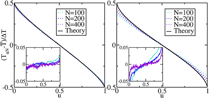
Figure 14. Rescaled temperature profile for resonant BCs R = 0 (left) and free BCs with (right). In the main plots results of Monte-Carlo simulations for increasing system sizes N = 100, 200, and 400 are compared to the theoretical predictions given by Equation (118) for the R = 0 case (left panel) and the numerical solution of Equations (103, 112) with for the plots in the right panel. In the insets the differences between measurements and theory are shown. The other parameter values are T+ = 1.5, T− = 0.5, and ω = γ = 1 (adapted from Cividini et al. with permission from [36] Copyright SISSA Medialab Srl, IOP Publishing).
(ii) Perfectly reflecting case R → 1: As mentioned above this is equivalent to fixed BC for which the temperature profile, given in Equation (83), was computed from microscopic calculation in the previous section. In this case it is known [37] that the eigenfunctions of the operator are precisely the sine-functions αn(v), i.e.,
which is consistent with Equation (95). This then gives us the corresponding Green's function
Using this and Equations (114, 115) we recover the exact expressions for the temperature profile and current given in Equations (83, 85) [37].
For free BCs with λ ≠ ω we have 0 < R < 1. In this case it is difficult to solve Equations (103, 112) analytically but numerical solutions have been obtained. In Figure 14 (right panel) a comparison of the temperature profile obtained from the numerical solution and from direct microscopic simulations for R = 1/2 and one can observe excellent agreement. Note again that the temperature profile is singular at the boundaries. It turns out that the exponent μ characterizing this singularity depends on not only on α but also on R [66]. To determine this dependence we take a derivative with respect to v of Equation (103) and get . Although the integral is identically zero for all v, the individual terms in the integrand have divergences. For example, the kernel diverges as while diverges as |δv|μ−1. Requiring that all divergent integrals cancel each other, leads to the following relation between R and μ:
The integrals can be performed explicitly to give
which is plotted in Figure 15 along with results extracted from the temperature profile obtained from direct numerical solution of Equation (103). We note that this result differs from the one conjectured in [66] though rather interestingly, the values of μ at R = 0 and R = 1 obtained from the two expressions agree. A generalization of the above result for arbitrary α is possible using the Lévy walk approach with the general kernel in Equation (42) which leads to an expression similar to Equation (122), now with the right hand depending explicitly on α.
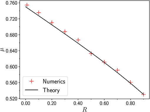
Figure 15. The meniscus exponent μ as a function of R for α = 1/2. The prediction from Equation (123) is plotted against the values obtained from the numerical solution of the integral Equation (103) with the kernel in Equation (112).
5. Summary and Open Questions
Heat transport in a large class of one-dimensional systems with Hamiltonian or conservative stochastic dynamics is known to be anomalous. Some typical signatures of anomalous transport include NESS studies which find that the thermal conductivity κ, diverges with system size N as κ ~ Nα, and the temperature profile T(x) is typically non-linear, with a singular dependence T(δx) ~ (δx)μ for small distance δx from the boundary. In the closed system one finds that heat pulses and correlation functions spread super-diffusively and are associated to propagators that have the scaling form . The scaling form is valid for times |x| < ct, where c is the sound speed in the system, beyond which time the correlations decay exponentially. The scaling function is given by the Lévy-stable distribution in the bulk and the finite cut-off leads to the width of the pulse scaling as σ(t) ~ tβ/2.
In this review we discussed these signatures of anomalous transport and showed how they can be understood within three different but related frameworks—(a) a phenomenological model where the heat carriers are taken to be Lévy walkers, (b) a microscopic phenomenological approach based on non-linear fluctuating hydrodynamics and (c) exact results obtained for certain stochastic models. The main picture that emerges is that anomalous heat transport can be understood by replacing Fourier's law in Equation (1) by a non-local fractional-type diffusion equation given in Equation (3), where the precise form of the kernel KR(x, y) depends on the specific set-up and boundary conditions. For the stochastic models the form of the kernel is known explicitly both for the closed system (infinite line) and the open system. In the Lévy walk picture, where the distribution of flight times has a power-law dependence ~1/tν+1, the kernel has the asymptotic form . We saw from the various approaches, that all the different exponents mentioned above are related to each other and in fact can be expressed in terms of the Lévy walk exponent as
For the Hamiltonian models that we discussed, namely the alternate mass hard-particle gas and the FPUT model, the various exponents are given by α = 1/3, β = 4/3, γ = 3/5 and correspond to a Lévy-walk exponent ν = 5/3. For the stochastic momentum exchange model we have α = 1/2, β = 3/2, γ = 2/3 which corresponds to ν = 3/2. The meniscus exponent μ is non-universal and depends on ν and on boundary conditions through a single dimensionless number R, which can be interpreted as the reflection coefficient of the Lévy walkers at the boundaries. In the context of the exactly solvable stochastic models, we discussed the spectrum of the fractional-type Laplacian operator [specified by the kernel KR(x, y)] in the open set-up, and pointed out important differences with the spectrum of the usual Laplacian for diffusive processes.
We conclude by mentioning some outstanding open questions in the field.
• Hamiltonian systems—The Lévy walk behavior has been clearly observed in large number of simulations. The formalism of NFH gives a microscopic justification of the Lévy walk model and the fractional-diffusion type description of the heat mode. Some open questions include:
1. A more rigorous microscopic derivation of the evolution equation of a localized heat pulse in an equilibrium system, to show that the central peak satisfies a fractional-diffusion type equation of a form similar to that in Equation (3).
2. Extension of the NFH formalism to the non-equilibrium case to study transport in finite open system and understand the role of BCs. Detailed simulations are also required to understand the effect of BCs.
3. Establishing the Lévy walk picture from a microscopic viewpoint?
• Stochastic systems—For the HCME model, the non-local version of Fourier's law has been established and the response kernel KR computed so far using two methods: (i) exact microscopic method for the BC corresponding to R = 1 and (ii) using NFH for arbitrary R. Is it possible to extend the exact microscopic approach to find the non-local kernel KR for general boundary conditions. Similarly for the HCVE it would be interesting to explore the role of BCs.
• For the HCME model, it has been possible to find the eigenspectrum of the non-local kernel KR for the case R = 1 and it was observed that the eigenvalues for Dirichlet and Neumann boundary conditions differ (unlike for the usual Laplacian). Finding the spectrum of the non-local kernel KR for general R, for Dirichlet and Neumann boundary conditions, is an interesting mathematical problem. The knowledge of the spectrum, namely eigenvectors and eigenvalues, enables one to study the time-evolution.
• For the HCME model we showed that it is possible to write a stochastic non-local equation (Equation 98) to describe equilibrium fluctuations. An open problem is to write such an equation in the non-equilibrium set-up. For diffusive systems this is given by Equation (97) and this equation enables one to compute long-range correlations in the NESS and large deviation functions.
Author Contributions
All authors listed have made a substantial, direct and intellectual contribution to the work, and approved it for publication.
Conflict of Interest
The authors declare that the research was conducted in the absence of any commercial or financial relationships that could be construed as a potential conflict of interest.
Acknowledgments
AnK would like to acknowledge the support from DST grant under project No. ECR/2017/000634. AD would like to acknowledge support of the project EDNHS ANR-14-CE25-0011 of the French National Research Agency (ANR). AnK and AD would like to acknowledge the support from the project 5604-2 of the Indo-French Centre for the Promotion of Advanced Research (IFCPAR).
References
1. Bonetto F, Lebowitz JL, Rey-Bellet L. Fourier's law: a challenge to theorists. In: A. Fokas, A. Grigoryan, T. Kibble, B. Zegarlinski, editors. Mathematical Physics 2000. Imperial College London; World Scientific (2000). p. 128–50. doi: 10.1142/9781848160224_0008
2. Lepri S, Livi R, Politi A. Thermal conduction in classical low-dimensional lattices. Phys Rep. (2003) 377:1–80. doi: 10.1016/S0370-1573(02)00558-6
3. Dhar A. Heat transport in low-dimensional systems. Adv Phys. (2008) 57:457–537. doi: 10.1080/00018730802538522
4. Lepri S editor. Thermal Transport in Low Dimensions: From Statistical Physics to Nanoscale Heat Transfer. Vol. 921. Heidelberg: Springer (2016).
5. Lepri S, Livi R, Politi A. Heat conduction in chains of nonlinear oscillators. Phys Rev Lett. (1997) 78:1896.
6. Dhar A. Heat conduction in a one-dimensional gas of elastically colliding particles of unequal masses. Phys Rev Lett. (2001) 86:3554–7. doi: 10.1103/PhysRevLett.86.3554
7. Grassberger P, Nadler W, Yang L. Heat conduction and entropy production in a one-dimensional hard-particle gas. Phys Rev Lett. (2002) 89:180601. doi: 10.1103/PhysRevLett.89.180601
8. Cipriani P, Denisov S, Politi A. From anomalous energy diffusion to Levy walks and heat conductivity in one-dimensional systems. Phys Rev Lett. (2005) 94:244301. doi: 10.1103/PhysRevLett.94.244301
9. Basile G, Bernardin C, Olla S. Momentum conserving model with anomalous thermal conductivity in low dimensional systems. Phys Rev Lett. (2006) 96:1–4. doi: 10.1103/PhysRevLett.96.204303
10. Mai T, Dhar A, Narayan O. Equilibration and universal heat conduction in fermi-pasta-ulam chains. Phys Rev Lett. (2007) 98:184301. doi: 10.1103/PhysRevLett.98.184301
11. Dhar A, Saito K. Heat conduction in the disordered Fermi-Pasta-Ulam chain. Phys Rev E. (2008) 78:061136. doi: 10.1103/PhysRevE.78.061136
12. Chen S, Wang J, Casati G, Benenti G. Nonintegrability and the Fourier heat conduction law. Phys Rev E. (2014) 90:032134. doi: 10.1103/PhysRevE.90.032134
13. Chang CW, Okawa D, Garcia H, Majumdar A, Zettl A. Breakdown of Fourier's law in nanotube thermal conductors. Phys Rev Lett. (2008) 101:075903. doi: 10.1103/PhysRevLett.101.075903
14. Xu X, Pereira LF, Wang Y, Wu J, Zhang K, Zhao X, et al. Length-dependent thermal conductivity in suspended single-layer graphene. Nat Commun. (2014) 5:3689. doi: 10.1038/ncomms4689
15. Lee V, Wu CH, Lou ZX, Lee WL, Chang CW. Divergent and ultrahigh thermal conductivity in millimeter-long nanotubes. Phys Rev Lett. (2017) 118:135901. doi: 10.1103/PhysRevLett.118.135901
16. Majee AK, Aksamija Z. Length divergence of the lattice thermal conductivity in suspended graphene nanoribbons. Phys Rev B. (2016) 93:235423. doi: 10.1103/PhysRevB.93.235423
17. Pereira LFC, Donadio D. Divergence of the thermal conductivity in uniaxially strained graphene. Phys Rev B. (2013) 87:125424. doi: 10.1103/PhysRevB.87.125424
18. Nika DL, Askerov AS, Balandin AA. Anomalous size dependence of the thermal conductivity of graphene ribbons. Nano Lett. (2012) 12:3238–44. doi: 10.1021/nl301230g
19. Xu Z. Heat transport in low-dimensional materials: a review and perspective. Theor Appl Mech Lett. (2016) 6:113–21. doi: 10.1016/j.taml.2016.04.002
20. Meier T, Menges F, Nirmalraj P, Hölscher H, Riel H, Gotsmann B. Length-dependent thermal transport along molecular chains. Phys Rev Lett. (2014) 113:060801. doi: 10.1103/PhysRevLett.113.060801
21. Zhao H. Identifying diffusion processes in one-dimensional lattices in thermal equilibrium. Phys Rev Lett. (2006) 96:140602. doi: 10.1103/PhysRevLett.96.140602
22. Mendl CB, Spohn H. Dynamic correlators of fermi-pasta-ulam chains and nonlinear fluctuating hydrodynamics. Phys Rev Lett. (2013) 111:230601. doi: 10.1103/PhysRevLett.111.230601
23. Green MS. Markoff random processes and the statistical mechanics of time-dependent phenomena. II. Irreversible processes in fluids. J Chem Phys. (1954) 22:398–413.
24. Kubo R. Statistical-mechanical theory of irreversible processes. I. General theory and simple applications to magnetic and conduction problems. J Phys Soc Jpn. (1957) 12:570–86.
25. Jara M, Komorowski T, Olla S. Limit theorems for additive functionals of a Markov chain. Ann Appl Probab. (2009) 19:2270–300. doi: 10.1214/09-AAP610
26. Lepri S, Mejía-Monasterio C, Politi A. A stochastic model of anomalous heat transport: analytical solution of the steady state. J Phys A Math Theor. (2009) 42:025001. doi: 10.1088/1751-8113/42/2/025001
27. Lepri S, Mejia Monasterio C, Politi A. Nonequilibrium dynamics of a stochastic model of anomalous heat transport. J Phys A Math Theor. (2010) 43:065002.
28. Delfini L, Lepri S, Livi R, Mejía-Monasterio C, Politi A. Nonequilibrium dynamics of a stochastic model of anomalous heat transport: numerical analysis. J Phys A Math Theor. (2010) 43:145001. doi: 10.1088/1751-8113/43/14/145001
29. Jara M, Komorowski T, Olla S. Superdiffusion of energy in a chain of harmonic oscillators with noise. Commun Math Phys. (2015) 339:407–53. doi: 10.1007/s00220-015-2417-6
30. Bernardin C, Stoltz G. Anomalous diffusion for a class of systems with two conserved quantities. Nonlinearity. (2012) 25:1099–133. doi: 10.1088/0951-7715/25/4/1099
31. Bernardin C, Gonçalves P, Jara M. 3/4-Fractional superdiffusion in a system of harmonic oscillators perturbed by a conservative noise. Arch Rational Mech Anal. (2016) 220:505–42. doi: 10.1007/s00205-015-0936-0
32. Mellet A, Mischler S, Mouhot C. Fractional diffusion limit for collisional kinetic equations. Arch Rational Mech Anal. (2011) 199:493–525. doi: 10.1007/s00205-010-0354-2
33. Basile G, Bernardin C, Olla S. Thermal conductivity for a momentum conservative model. Commun Math Phys. (2009) 287:67–98. doi: 10.1007/s00220-008-0662-7
34. Priyanka Kundu A, Dhar A, Kundu A. Anomalous heat equation in a system connected to thermal reservoirs. Phys Rev E. (2018) 98:042105. doi: 10.1103/PhysRevE.98.042105
35. Miron A, Cividini J, Kundu A, Mukamel D. Derivation of fluctuating hydrodynamics and crossover from diffusive to anomalous transport in a hard-particle gas. Phys Rev E. (2019) 99:012124. doi: 10.1103/PhysRevE.99.012124
36. Cividini J, Kundu A, Miron A, Mukamel D. Temperature profile and boundary conditions in an anomalous heat transport model. J Stat Mech Theory Exp. (2017) 013203. doi: 10.1088/1742-5468/aa5337
37. Kundu A, Bernardin C, Saito K, Kundu A, Dhar A. Fractional equation description of an open anomalous heat conduction set-up. J Stat Mech Theory Exp. (2019) 2019:013205. doi: 10.1088/1742-5468/aaf630
38. Lepri S, Livi R, Politi A. On the anomalous thermal conductivity of one-dimensional lattices. Europhys Lett. (1998) 43:271.
39. Delfini L, Lepri S, Livi R, Politi A. Anomalous kinetics and transport from 1D self-consistent mode-coupling theory. J Stat Mech Theory Exp. (2007) 2007:P02007. doi: 10.1088/1742-5468/2007/02/P02007
40. Lepri S. Relaxation of classical many-body Hamiltonians in one dimension. Phys Rev E. (1998) 58:7165–71. doi: 10.1103/PhysRevE.58.7165
41. Lepri S, Livi R, Politi A. Universality of anomalous one-dimensional heat conductivity. Phys Rev E. (2003) 68:067102. doi: 10.1103/PhysRevE.68.067102
42. Delfini L, Lepri S, Livi R, Politi A. Self-consistent mode-coupling approach to one-dimensional heat transport. Phys Rev E. (2006) 73:060201. doi: 10.1103/PhysRevE.73.060201
43. Wang JS, Li B. Intriguing heat conduction of a chain with transverse motions. Phys Rev Lett. (2004) 92:074302. doi: 10.1103/PhysRevLett.92.074302
44. Wang JS, Li B. Mode-coupling theory and molecular dynamics simulation for heat conduction in a chain with transverse motions. Phys Rev E. (2004) 70:021204. doi: 10.1103/PhysRevE.70.021204
45. Pereverzev A. Fermi-Pasta-Ulam β lattice: Peierls equation and anomalous heat conductivity. Phys Rev E. (2003) 68:056124. doi: 10.1103/PhysRevE.68.056124
46. Lukkarinen J, Spohn H. Anomalous energy transport in the FPU-β chain. Commun Pure Appl Math. (2008) 61:1753–86. doi: 10.1002/cpa.20243
47. van Beijeren H. Exact results for anomalous transport in one-dimensional Hamiltonian systems. Phys Rev Lett. (2012) 108:180601. doi: 10.1103/PhysRevLett.108.180601
48. Casati G, Prosen T. Anomalous heat conduction in a one-dimensional ideal gas. Phys Rev E. (2003) 67:015203. doi: 10.1103/PhysRevE.67.015203
49. Prosen T, Campbell DK. Normal and anomalous heat transport in one-dimensional classical lattices. Chaos. (2005) 15:015117. doi: 10.1063/1.1868532
50. Li B, Wang L, Casati G. Thermal diode: rectification of heat flux. Phys Rev Lett. (2004) 93:184301. doi: 10.1103/PhysRevLett.93.184301
51. Wang L, Wang T. Power-law divergent heat conductivity in one-dimensional momentum-conserving nonlinear lattices. Europhys Lett. (2011) 93:54002. doi: 10.1209/0295-5075/93/54002
52. Tamaki S, Sasada M, Saito K. Heat transport via low-dimensional systems with broken time-reversal symmetry. Phys Rev Lett. (2017) 119:110602. doi: 10.1103/PhysRevLett.119.110602
53. Saito K, Sasada M. Thermal conductivity for coupled charged harmonic oscillators with noise in a magnetic field. Commun Math Phys. (2018) 361:951–95. doi: 10.1007/s00220-018-3198-5
54. Li B, Wang J. Anomalous heat conduction and anomalous diffusion in one-dimensional systems. Phys Rev Lett. (2003) 91:044301. doi: 10.1103/PhysRevLett.91.044301
55. Chen S, Zhang Y, Wang J, Zhao H. Connection between heat diffusion and heat conduction in one-dimensional systems. Sci China Phys Mech Astron. (2013) 56:1466–71. doi: 10.1007/s11433-013-5163-9
56. Wang L, Wu Z, Xu L. Super heat diffusion in one-dimensional momentum-conserving nonlinear lattices. Phys Rev E. (2015) 91:062130. doi: 10.1103/PhysRevE.91.062130
57. Zaburdaev V, Denisov S, Hänggi P. Perturbation spreading in many-particle systems: a random walk approach. Phys Rev Lett. (2011) 106:180601. doi: 10.1103/PhysRevLett.106.180601
58. Li Y, Liu S, Li N, Hanggi P, Li B. 1D momentum-conserving systems: the conundrum of anomalous versus normal heat transport. New J Phys. (2015) 17:043064. doi: 10.1088/1367-2630/17/4/043064
59. Liu S, Hänggi P, Li N, Ren J, Li B. Anomalous heat diffusion. Phys Rev Lett. (2014) 112:040601. doi: 10.1103/PhysRevLett.112.040601
60. Narayan O, Ramaswamy S. Anomalous heat conduction in one-dimensional momentum-conserving systems. Phys Rev Lett. (2002) 89:200601. doi: 10.1103/PhysRevLett.89.200601
61. Spohn H. Nonlinear fluctuating hydrodynamics for anharmonic chains. J Stat Phys. (2014) 154:1191–227. doi: 10.1007/s10955-014-0933-y
62. Spohn H, Stoltz G. Nonlinear fluctuating hydrodynamics in one dimension: the case of two conserved fields. J Stat Phys. (2015) 160:861–84. doi: 10.1007/s10955-015-1214-0
63. Das SG, Dhar A, Saito K, Mendl CB, Spohn H. Numerical test of hydrodynamic fluctuation theory in the Fermi-Pasta-Ulam chain. Phys Rev E. (2014) 90:012124. doi: 10.1103/PhysRevE.90.012124
64. Deutsch J, Narayan O. One-dimensional heat conductivity exponent from a random collision model. Phys Rev E. (2003) 68:010201. doi: 10.1103/PhysRevE.68.010201
65. Roy D. Crossover from Fermi-Pasta-Ulam to normal diffusive behavior in heat conduction through open anharmonic lattices. Phys Rev E. (2012) 86:041102. doi: 10.1103/PhysRevE.86.041102
66. Lepri S, Politi A. Density profiles in open superdiffusive systems. Phys Rev E. (2011) 83:030107. doi: 10.1103/PhysRevE.83.030107
67. Kundu A, Dhar A, Narayan O. The Green-Kubo formula for heat conduction in open systems. J Stat Mech Theory Exp. (2009) 03:L03001. doi: 10.1088/1742-5468/2009/03/L03001
68. Denisov S, Klafter J, Urbakh M. Dynamical heat channels. Phys Rev Lett. (2003) 91:194301. doi: 10.1103/PhysRevLett.91.194301
69. Dhar A, Saito K, Derrida B. Exact solution of a Lévy walk model for anomalous heat transport. Phys Rev E. (2013) 87:010103. doi: 10.1103/PhysRevE.87.010103
70. Dhar A, Saito K. Anomalous transport and current fluctuations in a model of diffusing Levy walkers. arXiv (2013) arXiv:13085476.
71. Dhar A, Saito K, Roy A. Energy current cumulants in one-dimensional systems in equilibrium. Phys Rev Lett. (2018) 120:220603. doi: 10.1103/PhysRevLett.120.220603
72. Klafter J, Zumofen G. Dynamically generated enhanced diffusion: the stationary state case. Phys A. (1993) 196:102–15.
73. Zumofen G, Klafter J. Scale-invariant motion in intermittent chaotic systems. Phys Rev E. (1993) 47:851–63.
74. Metzler R, Compte A. Stochastic foundation of normal and anomalous Cattaneo-type transport. Phys A. (1999) 268:454–68.
75. Buldyrev SV, Havlin S, Kazakov AY, da Luz MGE, Raposo EP, Stanley HE, et al. Average time spent by Lévy flights and walks on an interval with absorbing boundaries. Phys Rev E. (2001) 64:041108. doi: 10.1103/PhysRevE.64.041108
76. Miron A. Levy walks on finite intervals: a step beyond asymptotics. arXiv (2019) arXiv:190208974.
77. Prähofer M, Spohn H. Exact scaling functions for one-dimensional stationary KPZ growth. J Stat Phys. (2004) 115:255–79. doi: 10.1023/B:JOSS.0000019810.21828.fc
78. Prahofer. Available online at: https://www-m5.ma.tum.de/KPZ
79. Mellet A, Merino-Aceituno S. Anomalous energy transport in FPU-β chain. J Stat Phys. (2015) 160:583–621. doi: 10.1007/s10955-015-1273-2
80. Zoia A, Rosso A, Kardar M. Fractional Laplacian in bounded domains. Phys Rev E. (2007) 76:021116. doi: 10.1103/PhysRevE.76.021116
81. Buldyrev SV, Gitterman M, Havlin S, Kazakov AY, Da Luz MGE, Raposo EP, et al. Properties of Lévy flights on an interval with absorbing boundaries. Phys A. (2001) 302:148–61. doi: 10.1016/S0378-4371(01)00461-7
82. Chen W, Holm S. Fractional Laplacian time-space models for linear and nonlinear lossy media exhibiting arbitrary frequency power-law dependency. J Acoust Soc Am. (2004) 115:1424–30. doi: 10.1121/1.1646399
83. Derrida B. Non-equilibrium steady states: fluctuations and large deviations of the density and of the current. J Stat Mech. (2007) 2007:P07023. doi: 10.1088/1742-5468/2007/07/P07023
84. Bertini L, De Sole A, Gabrielli D, Jona-Lasinio G, Landim C. Macroscopic fluctuation theory. Rev Mod Phys. (2015) 87:593–636. doi: 10.1103/RevModPhys.87.593
85. Bertini L, De Sole A, Gabrielli D, Jona-Lasinio G, Landim C. Macroscopic fluctuation theory for stationary non-equilibrium states. J Stat Phys. (2002) 107:635–75. doi: 10.1023/A:1014525911391
Keywords: fractional diffusion equation, Levy walks, anomalous heat transport, fluctuating hydrodynamics, heat conduction
Citation: Dhar A, Kundu A and Kundu A (2019) Anomalous Heat Transport in One Dimensional Systems: A Description Using Non-local Fractional-Type Diffusion Equation. Front. Phys. 7:159. doi: 10.3389/fphy.2019.00159
Received: 18 June 2019; Accepted: 30 September 2019;
Published: 05 November 2019.
Edited by:
Carlos Mejía-Monasterio, Polytechnic University of Madrid, SpainReviewed by:
Stefano Lepri, Italian National Research Council (CNR), ItalyTarcísio Marciano Rocha Filho, University of Brasilia, Brazil
Copyright © 2019 Dhar, Kundu and Kundu. This is an open-access article distributed under the terms of the Creative Commons Attribution License (CC BY). The use, distribution or reproduction in other forums is permitted, provided the original author(s) and the copyright owner(s) are credited and that the original publication in this journal is cited, in accordance with accepted academic practice. No use, distribution or reproduction is permitted which does not comply with these terms.
*Correspondence: Anupam Kundu, YW51cGFtLmt1bmR1QGljdHMucmVzLmlu