On the Spectra of One-Dimensional Schrödinger Operators With Singular Potentials

The paper is devoted to the spectral properties of one-dimensional Schrödinger operators

$\begin{array}{ll}{S}_{q}u(x)=\left(-\frac{d^2}{d{x}^2}+q(x)\right)u(x),x\in ℝ,& (1)\end{array}$

with potentials q = q₀+q_s, where $q_0\in L^{\infty }(ℝ)$ is a regular potential, and $q_s\in {{D}}^{\prime }(ℝ)$ is a singular potential with support on a discrete infinite set ${Y}\subset ℝ$. We consider the extension ${H}$ of formal operator (1) to an unbounded operator in L²(ℝ) defined by the Schrödinger operator S_q0 with regular potential q₀ and interaction conditions at the points of the set ${Y}$. We study the closedness and self-adjointness of ${H}$. If the set ${Y}\simeq \mathbb{Z}$ has a periodic structure we give the description of the essential spectrum of operator ${H}$ in terms of limit operators. For periodic potentials q₀ we consider the Floquet theory of ${H}$, and apply the spectral parameter power series method for determining the band-gap structure of the spectrum. We also consider the case when the regular periodic part of the potential is perturbed by a slowly oscillating at infinity term. We show that this perturbation changes the structure of the spectra of periodic operators significantly. This works presents several numerical examples to demonstrate the effectiveness of our approach.

1. Introduction

We consider formal one-dimensional Schrödinger operators

$\begin{array}{ll}{S}_{q}u(x)=\left(-\frac{d^2}{d{x}^2}+q(x)\right)u(x),x\in ℝ& (2)\end{array}$

with potentials q = q₀ + q_s, where $q_0\in L^{\infty }(ℝ)$ is a regular potential and $q_s\in {{D}}^{\prime }(ℝ)$ is a singular potential with support on an infinite discrete set ${Y}\subset ℝ$. The Schrödinger operator S_q is a far-reaching generalization of the well-known Kronig-Penney Hamiltonian

${H}=-\frac{d^2}{d{x}^2}+{\displaystyle \sum _{\gamma \in \mathbb{Z}}}\alpha \delta (x-\gamma ),\alpha \in ℝ$

describing the electron propagation in one-dimensional crystals [1, 2]. There exists an extensive literature devoted to the different spectral problems of one-dimensional Schrödinger operators with singular potentials (see, e.g., [3–9]).

Let ${Y}={\left\{y_j\right\}}_{j\in \mathbb{Z}}$ be a sequence of points y_j ∈ ℝ such that y_j < y_j+1 for every j ∈ ℤ, e_j = (y_j, y_j+1), j ∈ ℤ, and |e_j| = y_j+1 − y_j, j ∈ ℤ, is the length of e_j. We assume that

$0<{\displaystyle \underset{j\in \mathbb{Z}}{inf}}\left|e_j\right|\le {\displaystyle \underset{j\in \mathbb{Z}}{sup}}\left|e_j\right|<\infty .$

Let the formal Schrödinger operator (2) have the potential q = q₀ + q_s, where $q_0\in L^{\infty }(ℝ)$ and

$\begin{array}{ll}{q}_s(x)={\displaystyle \sum _{y\in {Y}}}\left(\alpha \left(y\right)\delta \left(x-y\right)+\beta \left(y\right){\delta }^{\prime }\left(x-y\right)\right)& (3)\end{array}$

is a singular potential, which is a distribution in ${{D}}^{\prime }(ℝ)$ with support at ${Y}$. We assume that the functions α(y), β(y) belong to the space $l^{\infty }({Y})$ with the norm $\parallel u{\parallel }_{l^{\infty }({Y})}={sup}_{y\in {Y}}|u(y)|$.

Note that the operator S_q coincides with the operator S_q0 on the space $C_0^{\infty }(ℝ\backslash {Y})$. Following the Kurasov paper [9] we consider the extension of $S_q{|}_{C_0^{\infty }(ℝ\backslash {Y})}$ to the unbounded operator ${{H}}_{q_0}$ in L²(ℝ) defined by the Schrödinger operator S_q0 with domain $\text{Dom}{{H}}_{q_0}={\tilde{H}}^2(\text{Γ})$, being

$\begin{array}{l}{\tilde{H}}^2(\text{Γ})=\left\{u\in H^2(\text{Γ}):\left(\begin{array}{l}u\left(y^{+}\right)\\ u^{\prime }\left(y^{+}\right)\end{array}\right)=\text{A}\left(y\right)\left(\begin{array}{l}u\left(y^{-}\right)\\ u^{\prime }\left(y^{-}\right)\end{array}\right),\forall y\in {Y}\right\},\end{array}$

where $\Gamma =ℝ\backslash {Y}={\bigcup }_{j\in \mathbb{Z}}{e}_j$, $H^2(\Gamma )={\oplus }_{j\in \mathbb{Z}}{H}^2(e_j)$, being $H^2(e_j)$ the Sobolev spaces of the order 2 on the intervals e_j, $u(y^{\pm })={lim}_{\epsilon \to +0}u(y\pm \epsilon )$, $u^{\prime }(y^{\pm })={lim}_{\epsilon \to +0}{u}^{\prime }(y\pm \epsilon )$, and

$\text{A}\left(y\right)=\left(\begin{array}{ll}{a}_{11}\left(y\right)& a_{12}\left(y\right)\\ a_{21}\left(y\right)& a_{22}\left(y\right)\end{array}\right)$

is a complex 2 × 2-matrix with entries $a_{ij}(y)\in l^{\infty }({Y})$, i, j = 1, 2. For potential (3) the matrix A(y) is of the form

$\text{A}\left(y\right)=\left(\begin{array}{ll}\frac{4-\alpha \left(y\right)\beta \left(y\right)}{4+\alpha \left(y\right)\beta \left(y\right)}& \frac{-4\beta \left(y\right)}{4+\alpha \left(y\right)\beta \left(y\right)}\\ \frac{4\alpha \left(y\right)}{4+\alpha \left(y\right)\beta \left(y\right)}& \frac{4-\alpha \left(y\right)\beta \left(y\right)}{4+\alpha \left(y\right)\beta \left(y\right)}\end{array}\right),\alpha \left(y\right)\beta \left(y\right)\ne -4,y\in {Y}.$

The following results are obtained in the paper:

1. We prove an a priori estimate for the operator S_q0 of the form

$\parallel u{\parallel }_{{\tilde{H}}^2(\text{Γ})}\le C\left(\parallel S_{q_0}u{\parallel }_{L^2(ℝ)}+\parallel u{\parallel }_{L^2(ℝ)}\right),u\in {\tilde{H}}^2(\text{Γ}).$

This estimate implies that the operator ${{H}}_{q_0}$ is closed. Moreover, if the potential q₀ and the entries of the matrix A (y) are real-valued such that det A (y) = 1 for every $y\in {Y}$, the operator ${{H}}_{q_0}$ is self-adjoint.

2. Let the set ${Y}$ of the singular points of the potential q to have a periodic structure. This means that the set ${Y}$ is invariant with respect to the group 𝔾 = ℓℤ, ℓ>0. Let {g_m} be a sequence of points of the group 𝔾 tending to ∞. We associate with {g_m} the operator-valued sequence $\left\{V_{-g_m}{{H}}_{q_0}{V}_{g_m}\right\}$. We define the limit operators ${{H}}_{q^g}$, which are the limits in some sense of the operator sequences $\left\{V_{-g_m}{{H}}_{q_0}{V}_{g_m}\right\}$, where V_hu(x) = u(x − h), x ∈ ℝ, h ∈ 𝔾 is the shift operator. Then we give the general description of the essential spectrum $\text{s}{\text{p}}_{\text{ess}}{{H}}_{q_0}$ in terms of the limit operators.

3. Let every sequence 𝔾 ∋ g_m → ∞ have a subsequence 𝔾 ∋ h_m → ∞ defining a limit operator ${{H}}_{q_0^h}$. Then we prove that

$\begin{array}{ll}{\text{sp}}_{\text{ess}}{{H}}_{q_0}={\displaystyle \bigcup _{{{H}}_{q_0^h}\in \text{Lim}({{H}}_{q_0})}}\text{sp}{{H}}_{q_0^h},& (4)\end{array}$

where $\text{Lim}({{H}}_{q_0})$ is the set of all limit operators of ${{H}}_{q_0}$.

4. Periodic structures. Let the potential q₀(x), x ∈ ℝ, and the matrix A(y), $y\in {Y}$, be periodic with respect to the group 𝔾 and real-valued. Moreover, we assume that det A (y) = 1 for all $y\in {Y}$. Then ${{H}}_{q_0}$ is a self-adjoint operator and formula (4) yields

$\text{s}{\text{p}}_{\text{ess}}{{H}}_{q_0}=\text{sp}{{H}}_{q_0}.$

On applying the Floquet transform we obtain that

$\text{sp}{{H}}_{q_0}=\left\{\text{λ}\in ℝ:\left|D(\text{λ})\right|\le 1\right\},$

where $D(\lambda )=\frac{1}{2}({\phi }_1(\ell ,\lambda )+{({\phi }_2)}_x^{\prime }(\ell ,\lambda ))$ is a function defined from a pair of linearly independent solutions φ₁, φ₂ of the Schrödinger equation S_q0u(x) = λu(x), x∈[0, ℓ), which satisfy the Cauchy conditions φ₁(0, λ) = 1, ${({\phi }_1)}_x^{\prime }(0,\lambda )=0$, φ₂(0, λ) = 0, ${({\phi }_2)}_x^{\prime }(0,\lambda )=1$, as well as interaction conditions at the points $y\in {{Y}}_0\subset [0,\ell )$. In the paper we obtain an explicit expression for function D in terms of monodromy matrices associated to the point interactions from the singular potential (3). Entries of monodromy matrices are calculated by means of the SPPS method [10], which allows to consider arbitrary regular potentials q₀ satisfying certain smoothness conditions. This approach in turn leads to an effective numerical method for calculating the edges of the spectral bands of Schrödinger operators ${{H}}_{q_0}$.

5. Slowly oscillating at infinity perturbations of periodic potentials. We say that a function a ∈ L^∞ (ℝ) is slowly oscillating at infinity and belongs to the class SO(ℝ) if

${\displaystyle \underset{x\to \infty }{lim}}{\displaystyle \underset{x^{\prime }\in K}{sup}}|a(x+x^{\prime })-a(x)|=0$

for every compact set K ⊂ ℝ. As above we assume that the set ${Y}$ is invariant with respect to the group 𝔾. We apply formula (4) for the investigation of the perturbation of the periodic operators ${{H}}_q$ by adding to the potential $q_0\in L^{\infty }(ℝ)$ a slowly oscillating term q₁ ∈ SO (ℝ). Let ${{H}}_{q_0}$ be a periodic operator with respect to the group 𝔾 given by the Schrödinger operator S_q0 with 𝔾-periodic real-valued potential q₀ and the 𝔾-periodic real matrices A(y) satisfying det A(y) = 1 for every $y\in {Y}$. We consider the operator ${{H}}_{q_0+q_1}$, where q₁ ∈ SO (ℝ) is a real-valued function. Note that the operator ${{H}}_{q_0}$has a band-gap spectrum

$\text{sp}{{H}}_{q_0}={\displaystyle \bigcup _{k=1}^{\infty }}\left[a_k,b_k\right],b_k\le a_{k+1},k\in \mathbb{N}.$

The limit operators of the operator ${{H}}_{q_0+q_1}$ are of the form ${{H}}_{q_0+q_1}^h={{H}}_{q_0+q_1^h}$, where $q_1^h\in ℝ$. Hence

$\text{sp}{{H}}_{q_0+q_1^h}={\displaystyle \bigcup _{k=1}^{\infty }}\left[a_k+q_1^h,b_k+q_1^h\right].$

Applying formula (4) we obtain the essential spectrum of the operator ${{H}}_{q_0+q_1}$ as

$\text{s}{\text{p}}_{\text{ess}}{{H}}_{q_0+q_1}={\displaystyle \bigcup _{k=1}^{\infty }}\left[a_k+m_{q_1},b_k+M_{q_1}\right],$

where $m_{q_1}=lim{inf}_{x\to \infty }{q}_1(x)$, $M_{q_1}=lim{sup}_{x\to \infty }{q}_1(x)$. Above formula shows that if the oscillation of q₁ at infinity is large enough, that is a_k+1 − b_k < M_q1 − m_q1, the gap (b_k, a_k+1) of the spectrum of periodic operator ${{H}}_{q_0}$ disappears in $\text{s}{\text{p}}_{\text{ess}}{{H}}_{q_0+q_1}$. Hence, the slowly oscillating perturbations of the periodic potentials can substantially change the structure of the essential spectrum of ${{H}}_{q_0}$.

6. Numerical calculation of the spectra of Schrödinger operator with periodic point interactions. We consider several examples for showing the application of the theory here presented, and calculate approximations of their corresponding spectra.

Notations

We will use the standard notations: C^∞ (ℝ) is the space of infinitely differentiable functions on ℝ, $C_b^{\infty }(ℝ)$ is a subspace of C^∞(ℝ) of functions with all bounded derivatives on ℝ, ${D}(ℝ)=C_0^{\infty }(ℝ)$ is a subspace of C^∞(ℝ) consisting of functions with compact support, ${{D}}^{\prime }(ℝ)$ is the space of distributions under ${D}(ℝ)$. We denote by H^s(ℝ), s ∈ ℝ, the Sobolev space with the norm

$\parallel u{\parallel }_{H^s(ℝ)}={\left({\displaystyle {\int }_{ℝ}}{(1+{\xi }^2)}^s|û(\xi ){|}^2\text{d}\xi \right)}^{1/2},$

where û(ξ) is the Fourier transform of u(x). If Ω ⊆ ℝ is an open set, then H^s (Ω) is the space of restrictions on Ω of functions on ℝ with the standard norm of restriction.

If exist, we denote the one-sided limits of f at x₀ by

$f(x_0^{-}):={\displaystyle \underset{\begin{array}{l}x\to x_0,\\ x<x_0\end{array}}{lim}}f(x),f(x_0^{+}):={\displaystyle \underset{\begin{array}{l}x\to x_0,\\ x>x_0\end{array}}{lim}}f(x),$

and by ${\left[f\right]}_{x_0}:=f(x_0^{+})-f(x_0^{-})$ the (finite) jump of f at x₀.

Let X, Y be Banach spaces, then ${B}(X,Y)$ is the space of all bounded linear operators acting from X into Y, and ${K}(X,Y)$ is a subspace of ${B}(X,Y)$ consisting of all compact operators acting from X into Y. If X = Y we simply write ${B}(X)$ and ${K}(X)$, respectively.

Let A be an unbounded closed operator in a Hilbert space H with domain Dom(A) dense in H. The essential spectrum sp_essA of operator A is the set of numbers λ ∈ ℂ for which the operator A − λ is not Fredholm as an unbounded operator in H. If A is self-adjoint in H then its discrete spectrum is given by sp_disA = spA\sp_essA, where spA denotes the spectrum of A.

2. One-Dimensional Schrödinger Operators With Point Interactions

In this section we consider one-dimensional Schrödinger operators with potentials involving a countable set of point interactions and investigate some of their functional properties such as closedness, self-adjointness, Fredholmness, as well as their essential spectrum.

2.1. A Self-Adjoint Extension of Schrödinger Operators With a Point Interaction

Let us consider a singular distribution

$\begin{array}{ll}{q}_s(x)=\alpha \delta (x)+\beta {\delta }^{\prime }(x),& (5)\end{array}$

which represents a point interaction with support at x = 0. By the definitions

$\delta (x)u(x)=\delta (u)\delta (x)=u(0)\delta (x),$

and

${\delta }^{\prime }(x)u(x)={\delta }^{\prime }(u){\delta }^{\prime }(x)=-u^{\prime }(0){\delta }^{\prime }(x),$

it follows that the action of q_s on the test functions in ${D}(ℝ)$ is defined by

$q_{s}u=\alpha u(0)\delta (x)-\beta u^{\prime }(0){\delta }^{\prime }(x).$

In the study of Schrödinger operators involving point interactions we define a space of discontinuous test functions at x = 0,

$D_0(ℝ):=C_0^{\text{∞}}\left(\overline{{ℝ}_{+}}\right)\oplus C_0^{\text{∞}}\left(\overline{{ℝ}_{-}}\right)$

where ℝ_±: = {x ∈ ℝ: x≷ 0}, and $C_0^{\infty }(\overline{{ℝ}_{\pm }})$ are the spaces of restrictions on $\overline{{ℝ}_{\pm }}$ of functions in $C_0^{\infty }(ℝ)$. Continuations of δ- and δ′-distributions on functions in D₀(ℝ) are defined as follows

$\begin{array}{l}\tilde{\delta }(u):=\frac{u\left(0^{+}\right)+u\left(0^{-}\right)}{2},{\tilde{\delta }}^{\prime }(u):=-\frac{u^{\prime }\left(0^{+}\right)+u^{\prime }\left(0^{-}\right)}{2},\\ u\in D_0(ℝ).\end{array}$

If $u\in {D}(ℝ)$ it follows that $\tilde{\delta }(u)=\delta (u)$ and ${\tilde{\delta }}^{\prime }(u)={\delta }^{\prime }(u)$.

Let us consider the formal one-dimensional Schrödinger operator

$\begin{array}{ll}{S}_{q}u(x)=\left(-\frac{d^2}{d{x}^2}+q(x)\right)u(x),x\in ℝ,& (6)\end{array}$

where q = q_s + q₀, with $q_0\in L^{\infty }(ℝ)$ as a regular potential, and $q_s\in {{D}}^{\prime }(ℝ)$ as a singular potential defined in (5). Note that operator S_q coincides with operator S_q0 on the space $C_0^{\infty }(ℝ\backslash \left\{0\right\})$. A domain Dom(S_q) of operator S_q as an unbounded operator in L²(ℝ) must consist of functions u∈L²(ℝ) such that $S_{q}u\in L^2(ℝ)$. This condition is fulfilled by functions u ∈ D₀ (ℝ) satisfying at the origin the following interaction conditions

$\left(\begin{array}{l}u\left(0^{+}\right)\\ u^{\prime }\left(0^{+}\right)\end{array}\right)={\text{A}}_0\left(\begin{array}{l}u\left(0^{-}\right)\\ u^{\prime }\left(0^{-}\right)\end{array}\right),{\text{A}}_0=\left(\begin{array}{ll}\frac{4-\alpha \beta }{4+\alpha \beta }& \frac{-4\beta }{4+\alpha \beta }\\ \frac{4\alpha }{4+\alpha \beta }& \frac{4-\alpha \beta }{4+\alpha \beta }\end{array}\right),\alpha \beta \ne -4,$

where matrix A₀ satisfies det A₀ = 1.

The embedding theorem for Sobolev space implies that if $u\in H^2(ℝ\backslash \left\{0\right\}):=H^2({ℝ}_{+})\oplus H^2({ℝ}_{-})$ the one-sided limits u(0^±), u′(0^±) exist, and the jumps [u]₀, ${\left[u^{\prime }\right]}_0$ are well defined. Let ${{H}}_{q_0}$ be the unbounded operator in L²(ℝ) defined by the Schrödinger operator $S_{q_0}=-\frac{d^2}{d{x}^2}+q_0$ with domain $\text{Dom}({{H}}_{q_0})={\tilde{H}}^2(ℝ\backslash \left\{0\right\})$ where

$\begin{array}{l}{\tilde{H}}^2(ℝ\backslash \left\{0\right\})=\left\{u\in H^2(ℝ\backslash \left\{0\right\}):\left(\begin{array}{l}u\left(0^{+}\right)\\ u^{\prime }\left(0^{+}\right)\end{array}\right)={\text{A}}_0\left(\begin{array}{l}u\left(0^{-}\right)\\ u^{\prime }\left(0^{-}\right)\end{array}\right)\right\}.\end{array}$

If $q_0\in L^{\infty }(ℝ)$ is a real-valued function, A₀ is a real 2 × 2-matrix, and det A₀ = 1, then ${{H}}_{q_0}$ is a self-adjoint operator. We will prove this result in a more general setting in forthcoming Theorem 2. Thus the unbounded operator ${{H}}_{q_0}$ generated by the Schrödinger operator S_q0 with domain ${\tilde{H}}^2(ℝ\backslash \left\{0\right\})$ is a self-adjoint extension of formal Schrödinger operator S_q0+qs.

Schrödinger operators involving point interactions of the form $q_s(x)=\alpha \delta (x)+\beta {\delta }^{\prime }(x)$ have been considered as norm resolvent approximations of certain families of Schrödinger operators with potentials depending on parameters tending to zero. The norm resolvent convergence of such families of operators was established and a class of solvable models that approximate the quantum systems was obtained in the works [11–13].

2.2. Properties of Schrödinger Operators With a Countable Set of Point Interactions

Let ${Y}={\left\{y_j\right\}}_{j\in \mathbb{Z}}$ be a sequence of real numbers such that y_j < y_j+1 for every j ∈ ℤ. We denote by e_j: = (y_j, y_j+1), j∈ℤ, the corresponding interval between a pair of adjacent points y_j and y_j+1. The interval e_j has a length |e_j|: = y_j+1 − y_j, such that

$0<{\displaystyle \underset{j\in \mathbb{Z}}{inf}}\left|e_j\right|\le {\displaystyle \underset{j\in \mathbb{Z}}{sup}}\left|e_j\right|<\infty .$

We denote

$\text{Γ}:=ℝ\backslash {Y}={\displaystyle \bigcup _{j\in \mathbb{Z}}}{e}_j,\mathrm{\text{and }}{H}^2(\text{Γ}):={\displaystyle \underset{j\in \mathbb{Z}}{\oplus }}{H}^2\left(e_j\right).$

Let us consider the Schrödinger operator S_q defined in (6) with the regular potential $q_0\in L^{\infty }(ℝ)$, and the singular potential

$\begin{array}{ll}{q}_s(x)={\displaystyle \sum _{y\in {Y}}}\left(\alpha \left(y\right)\delta \left(x-y\right)+\beta \left(y\right){\delta }^{\prime }\left(x-y\right)\right),& (7)\end{array}$

which is a distribution in ${{D}}^{\prime }(ℝ)$ with support at ${Y}\subset ℝ$. We assume that $\alpha ,\beta \in l^{\infty }({Y})$, where the space $l^{\infty }({Y})$ consists of all bounded complex-valued functions on the set ${Y}$, which is equipped by the norm $\parallel u{\parallel }_{l^{\infty }({Y})}:=\underset{y\in {Y}}{sup}|u(y)|$. Note that the operator S_q coincides with the Schrödinger operator $S_{q_0}:=-\frac{d^2}{d{x}^2}+q_0$ on the space $C_0^{\infty }(\Gamma ):={\oplus }_{j\in \mathbb{Z}}{C}_0^{\infty }(e_j)$. Following the ideas of the work [9], the operator S_q defined on $C_0^{\infty }(\Gamma )$ is extended to an unbounded operator ${{H}}_{q_0}$ in L²(ℝ) defined by the Schrödinger operator S_q0 with domain $\text{Dom}({{H}}_{q_0})={\tilde{H}}^2(\Gamma )$, where ${\tilde{H}}^2(\Gamma )$ is a subspace of H²(Γ) given by

$\begin{array}{l}{\tilde{H}}^2(\text{Γ})=\left\{u\in H^2(\text{Γ}):\left(\begin{array}{l}u\left(y^{+}\right)\\ u^{\prime }\left(y^{+}\right)\end{array}\right)=\text{A}\left(y\right)\left(\begin{array}{l}u\left(y^{-}\right)\\ u^{\prime }\left(y^{-}\right)\end{array}\right),\forall y\in {Y}\right\},\end{array}$

where

$\text{A}\left(y\right)=\left(\begin{array}{ll}{a}_{11}\left(y\right)& a_{12}\left(y\right)\\ a_{21}\left(y\right)& a_{22}\left(y\right)\end{array}\right),y\in {Y},$

are complex 2 × 2-matrices with entries $a_{ij}\in l^{\infty }({Y})$ (i, j = 1, 2). In the case of potential (7), the corresponding matrices are of the form

$\begin{array}{l}\text{A}\left(y\right):=\left(\begin{array}{ll}\frac{4-\alpha \left(y\right)\beta \left(y\right)}{4+\alpha \left(y\right)\beta \left(y\right)}& \frac{-4\beta \left(y\right)}{4+\alpha \left(y\right)\beta \left(y\right)}\\ \frac{4\alpha \left(y\right)}{4+\alpha \left(y\right)\beta \left(y\right)}& \frac{4-\alpha \left(y\right)\beta \left(y\right)}{4+\alpha \left(y\right)\beta \left(y\right)}\end{array}\right),\alpha \left(y\right)\beta \left(y\right)\ne -4,y\in {Y},\end{array}$

which satisfy det A (y) = 1, for every $y\in {Y}$.

If the conditions:

1. regular potential $q_0\in L^{\infty }(ℝ)$, and

2. matrices $\text{A}(y)={(a_{ij}(y))}_{i,j=1}^2$ are such that $a_{ij}\in l^{\infty }({Y})$ for every $y\in {Y}$

are fulfilled, then the operator S_q0 is bounded from ${\tilde{H}}^2(\Gamma )$ into L²(ℝ). Let us consider the following results for Schrödinger operators involving a countable set of point interactions.

Theorem 1 (An a priori estimate). Let $\underset{j\in \mathbb{Z}}{inf}\left|e_j\right|>0$, and conditions (1), (2) be satisfied. Then, there exists a constant C>0 such that for every function $u\in {\tilde{H}}^2(\Gamma )$ the following estimate

$\begin{array}{ll}\parallel u{\parallel }_{{\tilde{H}}^2(\text{Γ})}\le C\left(\parallel S_{q_0}u{\parallel }_{L^2(ℝ)}+\parallel u{\parallel }_{L^2(ℝ)}\right)& (8)\end{array}$

holds.

Proof. A priori estimate (8) is proved similarly as in the theory of general boundary-value problems (see, e.g., [14]), but instead of a finite partition of unity we use a countable partition of unity of finite multiplicity. The proof is similar to that of Theorem 3.1 in Rabinovich [15].

Theorem 1 implies the following propositions.

Proposition 1 (Closedness). Let conditions (1), (2) hold. Then, the operator ${{H}}_{q_0}$ is closed in L²(ℝ).

Proposition 2 (Parameter dependent Schrödinger operators). Let

$S_{{\mu }^2}u(x):=-\frac{d^{2}u(x)}{d{x}^2}+{\mu }^{2}u(x),x\in \text{Γ},\mu >0$

be a Schrödinger operator acting from ${\tilde{H}}^2(\Gamma )$ into L²(ℝ). We assume that the entries of matrices A(y), $y\in {Y}$, are real-valued, and liminf_{y → ∞}|a₁₂(y)| > 0 or there exists a finite set ${N}\subset {Y}$ such that a₁₂(y) = 0 for every $y\in {Y}\backslash {N}$. Then, there exists μ₀ > 0 such that the operator $S_{{\mu }^2}:{\tilde{H}}^2(\Gamma )\to L^2(ℝ)$ is invertible for every μ ≥ μ₀.

Proof: To prove this proposition we follow the approach of the well-known paper [16] where the authors studied general elliptic boundary-value problems depending on a parameter in bounded domains in ℝⁿ. Similarly to the proof of Theorem 1, here we use a partition of unity and construct local inverses depending on a parameter, and then we form the global inverse operator by sticking these inverses for large values of the parameter. Unlike the paper [16], here we use a countable partition of unity of finite multiplicity, and follow the proof of Proposition 2 in Rabinovich [17].

Theorem 2 (Self-adjointness). Let $q_0\in L^{\infty }(ℝ)$ be real-valued, and let matrices $\text{A}(y)={(a_{ij}(y))}_{i,j=1}^2$ possess real-valued entries $a_{ij}\in l^{\infty }({Y})$. We assume: (i) liminf_{y → ∞}|a₁₂(y)| > 0 or there exists a finite set ${N}\subset {Y}$ such that a₁₂(y) = 0 for every $y\in {Y}\backslash {N}$; (ii) det A(y) = 1, for every $y\in {Y}$. Then, the unbounded operator ${{H}}_{q_0}$ defined by the Schrödinger operator $S_{q_0}=-\frac{d^2}{d{x}^2}+q_0$ with domain ${\tilde{H}}^2(\Gamma )$ is self-adjoint in L²(ℝ).

Proof: Let $u,v\in \text{Dom}({{H}}_q)$. On applying integration by parts twice we obtain

${\displaystyle {\int }_{\text{Γ}}}{S}_{q}u(x)\overline{v}(x)\text{d}x={\displaystyle {\int }_{\text{Γ}}}u(x)S_q\overline{v}(x)\text{d}x+{\displaystyle \sum _{y\in {Y}}}\left({\left[u\overline{v^{\prime }}\right]}_y-{\left[u^{\prime }\overline{v}\right]}_y\right).$

Note that

$\begin{array}{l}{\left[u\overline{v^{\prime }}\right]}_y-{\left[u^{\prime }\overline{v}\right]}_y=\left(u\left(y^{+}\right)\overline{v^{\prime }}\left(y^{+}\right)-u\left(y^{-}\right)\overline{v^{\prime }}\left(y^{-}\right)\right)\\ -\left(u^{\prime }\left(y^{+}\right)\overline{v}\left(y^{+}\right)-u^{\prime }\left(y^{-}\right)\overline{v}\left(y^{-}\right)\right)\\ =\text{det}\left(\begin{array}{c}u\left(y^{+}\right)\overline{v}\left(y^{+}\right)\\ u^{\prime }\left(y^{+}\right)\overline{v^{\prime }}\left(y^{+}\right)\end{array}\right)-\text{det}\left(\begin{array}{cc}u\left(y^{-}\right)& \overline{v}\left(y^{-}\right)\\ u^{\prime }\left(y^{-}\right)& \overline{v^{\prime }}\left(y^{-}\right)\end{array}\right)\\ =\left(\text{det}\text{A}\left(y\right)-1\right)\text{det}\left(\begin{array}{c}u\left(y^{-}\right)\overline{v}\left(y^{-}\right)\\ u^{\prime }\left(y^{-}\right)\overline{v^{\prime }}\left(y^{-}\right)\end{array}\right)=0,\forall y\in {Y},\end{array}$

where we have used the condition det A (y) = 1. Hence, the operators $-\frac{d^2}{d{x}^2}$ and S_q0 with domain ${\tilde{H}}^2(\Gamma )$ are symmetric operators in L²(ℝ). It follows from Proposition 2 that there exists μ₀ > 0 such that $S_{q_0}+{\mu }_0^2:{\tilde{H}}^2(\Gamma )\to L^2(ℝ)$ is an isomorphism. To prove that ${{H}}_{q_0}+{\mu }_0^2$ with domain ${\tilde{H}}^2(\Gamma )$ is a self-adjoint operator in L²(ℝ) we have to show that $\text{Dom}({(S_{q_0}+{\mu }_0^2)}^{*})=\text{Dom}(S_{q_0}+{\mu }_0^2)$. Since $S_{q_0}+{\mu }_0^2$ is a symmetric operator $\text{Dom}(S_{q_0}+{\mu }_0^2)\subset \text{Dom}({(S_{q_0}+{\mu }_0^2)}^{*})$. Assume that $u\in \text{Dom}({(S_{q_0}+{\mu }_0^2)}^{*})$, then ${(S_{q_0}+{\mu }_0^2)}^{*}u=f\in L^2(ℝ)$. Since $S_{q_0}+{\mu }_0^2:\text{Dom}(S_{q_0})\to L^2(ℝ)$ is an isomorphism, there exists $v\in \text{Dom}(S_{q_0}+{\mu }_0^2)$ such that $(S_{q_0}+{\mu }_0^2)v=f$. Since $\text{Dom}(S_{q_0}+{\mu }_0^2)\subset \text{Dom}({(S_{q_0}+{\mu }_0^2)}^{*})$ we obtain that ${(S_{q_0}+{\mu }_0^2)}^{*}v=f$. Hence

$u-v\in ker{\left(S_{q_0}+{\mu }_0^2\right)}^{*}={\left(\text{Im}\left(S_{q_0}+{\mu }_0^2\right)\right)}^{\perp }=\left\{0\right\}.$

Therefore, $u=v\in \text{Dom}(S_{q_0}+{\mu }_0^2)$ and $\text{Dom}(S_{q_0}+{\mu }_0^2)=\text{Dom}({(S_{q_0}+{\mu }_0^2)}^{*})$. Thus, $S_{q_0}+{\mu }_0^2$ is a self-adjoint operator in L²(ℝ) with domain $\text{Dom}(S_{q_0})={\tilde{H}}^2(\Gamma )$. Note that the operator of multiplication by ${\mu }_0^2$ is strongly dominated by the operator S_q0 (see, e.g., [18, p. 73]). Hence, ${{H}}_{q_0}$ with domain ${\tilde{H}}^2(\Gamma )$ is a self-adjoint operator.

2.3. Fredholm Property and Essential Spectrum of Schrödinger Operators With Point Interactions

In this subsection we give the necessary and sufficient conditions of Fredholmness for Schrödinger operators $S_{q_0}:{\tilde{H}}^2(\Gamma )\to L^2(ℝ)$ with point interactions in terms of limit operators. We apply these results to the description of the essential spectrum of the corresponding unbounded operators ${{H}}_{q_0}$. Through this subsection we assume that the sequence of points ${Y}={\left\{y_j\right\}}_{j\in \mathbb{Z}}\subset ℝ$ where the singular potential q_s is supported is periodic with respect to the group 𝔾 = ℓℤ, ℓ > 0. We also assume that matrices ${Y}\ni y\mapsto \text{A}(y)$ are periodic with respect to 𝔾.

Definition 1. A potential $q_0\in L^{\infty }(ℝ)$ is said to be rich if for every sequence g = (g_m), 𝔾 ∋ g_m → ∞, there exists a subsequence h = (h_m), h_m → ∞, and a limit function $q_0^h\in L^{\infty }(ℝ)$ such that for every segment [a, b] ⊂ ℝ

${\displaystyle \underset{m\to \infty }{lim}}{\displaystyle \underset{x\in \left[a,b\right]}{sup}}|q_0^h(x)-q_0(x+h_m)|=0.$

Definition 2. The Schrödinger operator $S_{q_0^h}:{\tilde{H}}^2(\Gamma )\to L^2(ℝ)$ defined by

$S_{q_0^h}u(x):=\left(-\frac{d^2}{d{x}^2}+q_0^h(x)\right)u(x),x\in \text{Γ},$

with a limit function $q_0^h$ replacing the rich potential q₀ is called a limit operator of $S_{q_0}:{\tilde{H}}^2(\Gamma )\to L^2(ℝ)$. The set of all limit operators of S_q0 is denoted by Lim(S_q0).

Let $\phi \in C_0^{\infty }(ℝ)$ such that 0 ≤ φ(x) ≤ 1, where φ(x) = 1 if $\left|x\right|\le \frac{1}{2}$, and φ(x) = 0 if |x|≥1. Let φ_R(x) = φ(x/R), and ψ_R(x) = 1−φ_R(x).

Theorem 3. Let $q_0\in L^{\infty }(ℝ)$ be a rich potential, and let matrices ${Y}\ni y\mapsto \text{A}(y)$ be 𝔾-periodic. Then $S_{q_0}:{\tilde{H}}^2(\Gamma )\to L^2(ℝ)$ is a Fredholm operator if and only if all limit operators $S_{q_0^h}:{\tilde{H}}^2(\Gamma )\to L^2(ℝ)$ are invertible.

Proof: One can prove that the operator $S_{q_0}:{\tilde{H}}^2(\Gamma )\to L^2(ℝ)$ is locally Fredholm, that is for every R > 0 there exist operators ${{L}}_R,{{R}}_R\in {B}(L^2(ℝ),{\tilde{H}}^2(\Gamma ))$ such that

${{L}}_R{S}_{q_0}{\phi }_R={\phi }_R+T_R^{(1)},{\phi }_R{S}_{q_0}{{R}}_R={\phi }_R+T_R^{(2)},$

where $T_R^{(1)}\in {K}({\tilde{H}}^2(\Gamma ))$, and $T_R^{(2)}\in {K}(L^2(ℝ))$ since S_q0 is an elliptic operator. Hence, in order to prove that $S_{q_0}:{\tilde{H}}^2(\Gamma )\to L^2(ℝ)$ is a Fredholm operator we have to study the local invertibility of S_q0 at infinity, i.e., we have to prove that there exists R₀ > 0 and operators ${{L}}_{R_0}^{\infty },{{R}}_{R_0}^{\infty }\in {B}(L^2(ℝ),{\tilde{H}}^2(\Gamma ))$ such that

${{L}}_{R_0}^{\infty }{S}_{q_0}{\psi }_{R_0}={\psi }_{R_0},{\psi }_{R_0}{S}_{q_0}{{R}}_{R_0}^{\infty }={\psi }_{R_0}.$

Let μ₀ > 0 be such that the operator $S_{{\mu }_0^2}:{\tilde{H}}^2(\Gamma )\to L^2(ℝ)$ is an isomorphism. We set

${A}=S_{q_0}{S}_{{\mu }_0^2}^{-1}:L^2(ℝ)\to L^2(ℝ).$

It is easy to prove that $S_{q_0}:{\tilde{H}}^2(\Gamma )\to L^2(ℝ)$ is locally invertible at infinity if and only if ${A}$ is locally invertible at infinity. For the study of local invertibility at infinity we use the results of the book [19], and the work [20].

Let $\varphi \in C_b^{\infty }(ℝ)$, and ϕ_t(x) = ϕ(tx), t∈ℝ. Then it is easy to prove that

${\displaystyle \underset{t\to 0}{lim}}\parallel \left[{\varphi }_t,{A}\right]\parallel ={\displaystyle \underset{t\to 0}{lim}}\parallel {\varphi }_t{A}-{A}{\varphi }_t\parallel =0,$

that is, ${A}$ belongs to the C*-algebra of so-called band-dominated operators in L²(ℝ) (see, e.g., [20]). We introduce the limit operators of ${A}$ as follows. For 𝔾 ∋ h_m → ∞ let V_hmu(x): = u(x−h_m) be the corresponding sequence of shift operators. We say that ${{A}}^h$ is a limit operator defined by the sequence h = (h_m) if

$\begin{array}{l}\parallel \left(V_{-h_m}{A}{V}_{h_m}-{{A}}^h\right)\phi {\parallel }_{{B}(L^2(ℝ))}\\ =\parallel \phi \left(V_{-h_m}{A}{V}_{h_m}-{{A}}^h\right){\parallel }_{{B}(L^2(ℝ))}=0& (9)\end{array}$

for every $\phi \in C_0^{\infty }(ℝ)$. One can see that

$\begin{array}{ll}{V}_{-h_m}{A}{V}_{h_m}=V_{-h_m}{{H}}_{q_0}{V}_{h_m}{S}_{{\mu }_0^2}^{-1}.& (10)\end{array}$

Formulas (9), (10) imply that

${{A}}^h=S_{q_0^h}{S}_{{\mu }_0^2}^{-1}.$

Moreover, since the potential q₀ is rich the operator ${A}$ is rich, that is, every sequence g = (g_m) of 𝔾 tending to infinity has a subsequence h = (h_m) tending to infinity that defines the limit operator ${{A}}^h$. It follows from the results of Rabinovich et al. [19] and Lindner and Seidel [20] that the operator ${A}$ is locally invertible at infinity if and only if all limit operators ${{A}}^h$ are invertible. Since $S_{{\mu }_0^2}:{\tilde{H}}^2(\Gamma )\to L^2(ℝ)$ is an isomorphism, this yields the statement of the theorem.

Theorem 3 leads to the following description of the essential spectrum of operator ${{H}}_{q_0}$.

Theorem 4. Let $q_0\in L^{\infty }(ℝ)$ be a rich potential, and let the matrices ${Y}\ni y\mapsto \text{A}(y)$ be 𝔾-periodic. Then

$\begin{array}{ll}{\text{sp}}_{\text{ess}}{{H}}_{q_0}={\displaystyle \bigcup _{{{H}}_{q_0^h}\in \text{Lim}({{H}}_{q_0})}}\text{sp}{{H}}_{q_0^h},& (11)\end{array}$

where ${{H}}_{q_0^h}$ is the limit operator of ${{H}}_{q_0}$ defined as an unbounded operator in L²(ℝ), generated by the Schrödinger operator $S_{q_0^h}$ with domain ${\tilde{H}}^2(\Gamma )$.

3. Spectral Analysis of Periodic Schrödinger Operators With Point Interactions

In this section we study the band-gap spectra of periodic Schrödinger operators with point interactions by using the Floquet transform (see e.g., [21]). We also analyze the case when the regular potential q₀ is perturbed by a slowly oscillating at infinity term by means of the limit operators method, and provide expressions for the essential spectrum of corresponding Schrödinger operator.

3.1. Periodic Schrödinger Operators With Point Interactions

From now on we will assume that:

1. the sequence of points ${Y}={\left\{y_j\right\}}_{j\in \mathbb{Z}}\subset ℝ$ on which the singular potential q_s is supported is periodic with respect to the group 𝔾 = ℓℤ, ℓ>0;

2. the matrices $\text{A}(y)={(a_{ij}(y))}_{i,j=1}^2$ are periodic with respect to the group 𝔾, that is, A(y +g) = A (y) for every g ∈ 𝔾 and $y\in {Y}$. The entries $a_{ij}\in l^{\infty }({Y})$ of the matrices are such that det A (y) = 1 for every $y\in {Y}$; and

3. the potential q₀ is a real-valued, piecewise continuous function, periodic with respect to the group 𝔾.

Let Γ₀: = [0, ℓ), and 𝔹 = [−π/ℓ, π/ℓ) be the reciprocal unit cell (also known as Brillouin zone) of Γ₀. Let ${{Y}}_0:={Y}\cap {\Gamma }_0=\left\{y_1,\cdots ,y_n\right\}$ be the set of points of discontinuity inside Γ₀, which satisfy 0 < y₁ < ⋯ < y_n < ℓ. We also assume that the finite jumps [q₀]_yj, not necessarily zero, are well-defined.

From conditions (1–3) and Theorem 3 it follows that the operator ${{H}}_{q_0}$ with domain ${\tilde{H}}^2(\Gamma )$ is self-adjoint in L²(ℝ). Moreover, the operator S_q0 is invariant with respect to the shifts on the elements of the group 𝔾, that is

$\begin{array}{l}{V}_g{S}_{q_0}u(x)=-\frac{d^{2}u\left(x+g\right)}{d{x}^2}+q_0\left(x+g\right)u\left(x+g\right)\\ =-\frac{d^{2}u\left(x+g\right)}{d{x}^2}+q_0(x)u\left(x+g\right)=S_{q_0}{V}_{g}u(x),& \end{array}$

for every g ∈ 𝔾. Since V_gS_q0 = S_q0V_g, and from (11), it yields that $\text{s}{\text{p}}_{\text{ess}}{{H}}_{q_0}=\text{sp}{{H}}_{q_0}$, and $\text{s}{\text{p}}_{\text{dis}}{{H}}_{q_0}=\mathrm{\text{Ø}}$. In addition, the operator S_q0 is semi-bounded from below, that is

$\langle S_{q_0}u,u\rangle \ge m_{q_0}\parallel u{\parallel }_{L^2(ℝ)}^2,$

where $m_{q_0}:={inf}_{x\in ℝ}{q}_0(x)$. This implies that

$\text{sp}{{H}}_{q_0}\subset \left[m_{q_0},+\infty \right).$

We introduce the Hilbert space $H:=L^2({\Gamma }_0,L^2(𝔹))$ of vector-valued functions with components in $L^2({\Gamma }_0)$, which is equipped by the norm

$\parallel u{\parallel }_H={\left({\displaystyle {\int }_{{\text{Γ}}_0}}\parallel u(x,·){\parallel }_{L^2(\text{𝔹})}^2\text{d}x\right)}^{1/2}.$

The Floquet transform is the map ${F}:L^2(ℝ)\to H$ defined for functions f that decay sufficiently fast by

$\left({F}f\right)(x,\theta )=\tilde{f}(x,\theta ):=\frac{1}{\sqrt{2\pi }}{\displaystyle \sum _{\alpha \in \mathbb{Z}}}f(x-\alpha \ell )e^{\text{i}\alpha \theta },x\in ℝ,\theta \in \text{𝔹},$

where the parameter θ is often called the quasi-momentum. The Floquet transform is an isometry from L²(ℝ) to H, whose inverse is given by

$({{F}}^{-1}\tilde{f})(x)=\frac{1}{\sqrt{2\pi }}{\displaystyle {\int }_{\text{𝔹}}}\tilde{f}(x,\theta )\text{d}\theta .$

Let us consider the problem

$\begin{array}{ll}{{H}}_{q_0}u(x)=\text{λ}u(x),u\in {\tilde{H}}^2(\text{Γ}),& (12)\end{array}$

where λ ∈ ℝ is the spectral parameter. The Floquet transform applied to (12) gives a spectral problem depending on the parameter θ ∈ 𝔹, defined by the differential equation

$S_{q_0}\tilde{u}(x,\theta )=\text{λ}\tilde{u}(x,\theta ),x\in (0,\ell )\backslash {{Y}}_0,\theta \in \text{𝔹},$

with the interaction conditions at the discontinuity points

$\left(\begin{array}{c}\tilde{u}\left(y^{+},\theta \right)\\ {\tilde{u}}_x^{\prime }\left(y^{+},\theta \right)\end{array}\right)=\text{A}\left(y\right)\left(\begin{array}{c}\tilde{u}\left(y^{-},\theta \right)\\ {\tilde{u}}_x^{\prime }\left(y^{-},\theta \right)\end{array}\right),y\in {{Y}}_0,$

and the quasi-periodic conditions

$\tilde{u}(\ell ,\theta )=e^{\text{i}\theta \ell }\tilde{u}(0,\theta ),{\tilde{u}}_x^{\prime }(\ell ,\theta )=e^{\text{i}\theta \ell }{\tilde{u}}_x^{\prime }(0,\theta ).$

The operator $S_{q_0}={F}{S}_{q_0}{{F}}^{-1}$ is represented as the orthogonal sum

$\begin{array}{ll}{S}_{q_0}={F}{S}_{q_0}{{F}}^{-1}={\displaystyle \underset{\theta \in B}{\oplus }}{S}_{q_0}^{\theta },& (13)\end{array}$

where

$S_{q_0}^{\theta }u(x,\theta ):=-\frac{d^{2}u(x,\theta )}{d{x}^2}+q_0(x)u(x,\theta ),x\in (0,\ell )\backslash {{Y}}_0.$

For each θ ∈ 𝔹, the operator $S_{q_0}^{\theta }$ defines an unbounded operator ${{H}}_{q_0}^{\theta }$ in $L^2({\Gamma }_0)$ with domain $\text{Dom}({{H}}_{q_0}^{\theta })={\tilde{H}}^2({\Gamma }_0\backslash {{Y}}_0)$, where

$\begin{array}{l}{H}^2\left({\text{Γ}}_0\backslash {{Y}}_0\right)\hfill \\ =\{u\in H^2\left({\text{Γ}}_0\backslash {{Y}}_0\right):\left(\begin{array}{c}u\left(y^{+},\theta \right)\\ u_x^{\prime }\left(y^{+},\theta \right)\end{array}\right)=\text{A}(y)\left(\begin{array}{c}u\left(y^{-},\theta \right)\\ u_x^{\prime }\left(y^{-},\theta \right)\end{array}\right),y\in {{Y}}_0,\hfill \\ u(\ell ,\theta )=e^{i\theta \ell }u(0,\theta ),u_x^{\prime }(\ell ,\theta )=e^{i\theta \ell }{u}_x^{\prime }(0,\theta ),\theta \in \mathbb{B}\}.\hfill \end{array}$

Operators ${{H}}_{q_0}^{\theta }$, θ ∈ 𝔹, with domain ${\tilde{H}}^2({\Gamma }_0\backslash {{Y}}_0)$ have discrete spectra

$\text{sp}{{H}}_{q_0}^{\theta }=\left\{{\text{λ}}_1(\theta )<{\text{λ}}_2(\theta )<\cdots <{\text{λ}}_j(\theta )<\cdots \right\},$

where λ_j(θ) are continuous functions on 𝔹. Expression (13) implies that

$\begin{array}{ll}\text{sp}{{H}}_{q_0}={\displaystyle \bigcup _{\theta \in \text{𝔹}}}\text{sp}{{H}}_{q_0}^{\theta }.& (14)\end{array}$

If the image of the Brillouin zone 𝔹 under λ_j is [a_j, b_j], a_j ≤ b_j, j ∈ ℕ, then formula (14) gives

$\begin{array}{ll}\text{sp}{{H}}_{q_0}={\displaystyle \bigcup _{j=1}^{\infty }}\left[a_j,b_j\right],& (15)\end{array}$

that is, the spectrum of Schrödinger operator ${{H}}_{q_0}$ with 𝔾-periodic potential q₀ involving point interactions has a band-gap structure.

3.2. Spectral Analysis of Periodic Schrödinger Operators With Point Interactions

For each θ ∈ 𝔹 we define the spectral problem

${{H}}_{q_0}^{\theta }u(x,\theta )=\text{λ}(\theta )u(x,\theta ),u\in {\tilde{H}}^2({\text{Γ}}_0\backslash {{Y}}_0).$

Solutions of this problem are sought in the form

$u(x,\theta ;\text{λ})=C_1(\theta ,\text{λ}){\phi }_1(x,\text{λ})+C_2(\theta ,\text{λ}){\phi }_2(x,\text{λ}),$

where C₁, C₂ are arbitrary coefficients, and φ₁, φ₂ are linearly independent solutions of the Schrödinger equation

$S_{q_0}u=\text{λ}u,x\in (0,\ell )\backslash {{Y}}_0$

satisfying the interaction conditions

$\left(\begin{array}{c}u\left(y^{+}\right)\\ u_x^{\prime }\left(y^{+}\right)\end{array}\right)=\text{A}\left(y\right)\left(\begin{array}{c}u\left(y^{-}\right)\\ u_x^{\prime }\left(y^{-}\right)\end{array}\right),y\in {{Y}}_0,$

as well as the initial conditions

$\begin{array}{lll}\hfill {\phi }_1(0,\text{λ})=1,\hfill & \hfill {({\phi }_1)}_x^{\prime }(0,\text{λ})=0,\hfill & (\mathrm{16a})\end{array}$

$\begin{array}{lll}{\phi }_2(0,\text{λ})=0,\hfill & {({\phi }_2)}_x^{\prime }(0,\text{λ})=1.\hfill & (\mathrm{16b})\end{array}$

By the Liouville identity, the Wronskian of φ₁ and φ₂ satisfies

$\begin{array}{l}\text{ det}\left(\begin{array}{cc}{\phi }_1\left(0,\text{λ}\right)& {\phi }_2\left(0,\text{λ}\right)\\ {\left({\phi }_1\right)}_x^{\prime }\left(0,\text{λ}\right)& {\left({\phi }_2\right)}_x^{\prime }\left(0,\text{λ}\right)\end{array}\right)\\ =\text{det}\left(\begin{array}{cc}{\phi }_1\left(x,\text{λ}\right)& {\phi }_2\left(x,\text{λ}\right)\\ {\left({\phi }_1\right)}_x^{\prime }\left(x,\text{λ}\right)& {\left({\phi }_2\right)}_x^{\prime }\left(x,\text{λ}\right)\end{array}\right)=1,\\ \forall x\in \left[0,\ell \right]\backslash {{Y}}_0.\end{array}$

From the quasi-periodic property

$u(\ell ,\theta )=e^{\text{i}\theta \ell }u(0,\theta ),u_x^{\prime }(\ell ,\theta )=e^{\text{i}\theta \ell }{u}_x^{\prime }(0,\theta )$

we obtain the following system of equations

$\begin{array}{ll}{C}_1(\theta ,\text{λ}){\phi }_1(\ell ,\text{λ})+C_2(\theta ,\text{λ}){\phi }_2(\ell ,\text{λ})=e^{\text{i}\theta \ell }{C}_1(\theta ,\text{λ}),\hfill & (\mathrm{17a})\end{array}$

$\begin{array}{ll}{C}_1(\theta ,\text{λ}){({\phi }_1)}_x^{\prime }(\ell ,\text{λ})+C_2(\theta ,\text{λ}){({\phi }_2)}_x^{\prime }(\ell ,\text{λ})=e^{\text{i}\theta \ell }{C}_2(\theta ,\text{λ}),& (\mathrm{17b})\end{array}$

with C₁, C₂ as unknowns. System (17) implies that ${(\begin{array}{cc}{C}_1(\theta ,\lambda )& C_2(\theta ,\lambda )\end{array})}^{⊺}$ is an eigenvector of the monodromy matrix

$\text{M}(\text{λ})=\left(\begin{array}{cc}{\phi }_1\left(\ell ,\text{λ}\right)& {\phi }_2\left(\ell ,\text{λ}\right)\\ {\left({\phi }_1\right)}_x^{\prime }\left(\ell ,\text{λ}\right)& {\left({\phi }_2\right)}_x^{\prime }\left(\ell ,\text{λ}\right)\end{array}\right)$

associated to the eigenvalue μ: = e^iθℓ. In order for system (17) to possess non-trivial solutions its determinant must vanish, that is

$\text{det}\left(\begin{array}{cc}{\phi }_1\left(\ell ,\text{λ}\right)-\mu & {\phi }_2\left(\ell ,\text{λ}\right)\\ {\left({\phi }_1\right)}_x^{\prime }\left(\ell ,\text{λ}\right)& {\left({\phi }_2\right)}_x^{\prime }\left(\ell ,\text{λ}\right)-\mu \end{array}\right)=0$

This leads to the dispersion equation

$\begin{array}{ll}{\mu }^2-2\mu D(\text{λ})+1=0,& (18)\end{array}$

where

$\begin{array}{l}D(\text{λ}):=\frac{1}{2}\left({\phi }_1(\ell ,\text{λ})+{({\phi }_2)}_x^{\prime }(\ell ,\text{λ})\right).\hfill \end{array}$

Equation (18) has solutions of the form μ: = e^iθℓ, θ ∈ 𝔹, if and only if |D(λ)| ≤ 1. Hence, the spectrum of ${{H}}_{q_0}$ is given by

$\text{sp}{{H}}_{q_0}=\left\{\text{λ}\in ℝ:\left|D(\text{λ})\right|\le 1\right\},$

and the edges of the spectral bands of $\text{sp}{{H}}_{q_0}$ are solutions λ_edge ∈ ℝ of the equation

$\left|D({\text{λ}}_{\text{edge}})\right|=1.$

3.3. Periodic Potentials Perturbed by Slowly Oscillating at Infinity Terms

A function a ∈ L^∞ (ℝ) is slowly oscillating at infinity if the limit

${\displaystyle \underset{x\to \infty }{lim}}{\displaystyle \underset{y\in K}{sup}}|a(x+y)-a(x)|=0$

holds for every compact set K ⊂ ℝ. We denote by SO (ℝ) the class of such functions. One can prove (see, e.g., [19, Chap. 3.1]) that all limit functions a^h of a ∈ SO (ℝ) defined by the sequence 𝔾 ∋ h_m → ∞ are real constants.

Let us consider a Schrödinger operator ${{H}}_q:{\tilde{H}}^2(\Gamma )\to L^2(ℝ)$ with a perturbed potential q = q₀+q₁ consisting of a periodic part $q_0\in L^{\infty }(ℝ)$ satisfying conditions (3), and a real-valued perturbation q₁ ∈ SO (ℝ). The result of Theorem 4 can be used for analyzing the essential spectrum of ${{H}}_q$. Note that the spectrum of operator ${{H}}_{q_0}$ has a band-gap structure according to (15). The limit operators of ${{H}}_q={{H}}_{q_0+q_1}$ are of the form ${{H}}_{q^h}={{H}}_{q_0+q_1^h}$, where $q_1^h\in ℝ$. Therefore

$\text{sp}{{H}}_{q_0+q_1^h}={\displaystyle \bigcup _{j=1}^{\infty }}\left[a_j+q_1^h,b_j+q_1^h\right].$

On considering formula (11) and previous expression we obtain the essential spectrum of perturbed operator ${{H}}_q={{H}}_{q_0+q_1}$, that is

$\begin{array}{ll}{\text{sp}}_{\text{ess}}{{H}}_q={\displaystyle \bigcup _{j=1}^{\infty }}\left[a_j+m_{q_1}^{\infty },b_j+M_{q_1}^{\infty }\right],& (19)\end{array}$

where

$m_{q_1}^{\infty }:={\displaystyle \underset{x\to \infty }{lim inf}}{q}_1(x),M_{q_1}^{\infty }:={\displaystyle \underset{x\to \infty }{lim sup}}{q}_1(x).$

Formula (19) implies that some spectral bands of $\text{s}{\text{p}}_{\text{ess}}{{H}}_q$ may overlap depending on the intensity of the perturbation q₁. Let $\left(b_l+M_{q_1}^{\infty },a_{l+1}+m_{q_1}^{\infty }\right)$, l ∈ ℕ, be a gap of $\text{s}{\text{p}}_{\text{ess}}{{H}}_q$, hence if the relation

$\begin{array}{ll}{M}_{q_1}^{\infty }-m_{q_1}^{\infty }>a_{l+1}-b_l& (20)\end{array}$

holds the gap will disappear due to the merging of the adjacent bands. If condition (20) is satisfied for all l ∈ ℕ, all spectral gaps of $\text{s}{\text{p}}_{\text{ess}}{{H}}_q$ will disappear resulting a continuous spectrum, that is

$\text{s}{\text{p}}_{\text{ess}}{{H}}_q=\left[a_1+m_{q_1}^{\infty },+\infty \right),\mathrm{\text{and s}}{\text{p}}_{\text{dis}}{{H}}_q\subset \left[m_{q_0},a_1+m_{q_1}^{\infty }\right).$

4. Dispersion Equation for Periodic Schrödinger Operators With Point Interactions

In this section we determine the function D(λ) from a set of monodromy matrices specified at the points where the singular potential is supported in the fundamental domain Γ₀. We also apply the spectral parameter power series method [10] to derive a numerical method for calculating the spectral bands of Schrödinger operators ${{H}}_{q_0}$ with arbitrary regular potentials q₀ satisfying certain smoothness conditions.

4.1. Calculation of Function D(λ) in Terms of Monodromy Matrices

We begin by determining a general solution of the equation

$\begin{array}{ll}-\frac{d^{2}u(x)}{d{x}^2}+q_0(x)u(x)=\text{λ}u,x\in (0,\ell )\backslash {{Y}}_0,& (21)\end{array}$

satisfying the interaction conditions

$\begin{array}{l}\left(\begin{array}{l}u\left(y_j^{+}\right)\\ u^{\prime }\left(y_j^{+}\right)\end{array}\right)=\text{A}\left(y_j\right)\left(\begin{array}{l}u\left(y_j^{-}\right)\\ u^{\prime }\left(y_j^{-}\right)\end{array}\right),\\ \text{A}\left(y_j\right)=\left(\begin{array}{ll}\frac{4-{\alpha }_j{\beta }_j}{4+{\alpha }_j{\beta }_j}& \frac{-4{\beta }_j}{4+{\alpha }_j{\beta }_j}\\ \frac{4{\alpha }_j}{4+{\alpha }_j{\beta }_j}& \frac{4-{\alpha }_j{\beta }_j}{4+{\alpha }_j{\beta }_j}\end{array}\right),{\alpha }_j{\beta }_j\ne -4,\end{array}$

at the points of discontinuity $y_j\in {{Y}}_0$ (j = 1, ⋯ , n). By abusing the notation, we set y₀≡0, and y_n+1≡ℓ. The interval between two adjacent points of discontinuity y_j, y_j+1 is denoted by e_j = (y_j, y_j+1) (j = 0, ⋯ , n). Let ϕ_{1, j}, ϕ_{2, j} (j = 0, ⋯ , n) be a pair of linearly independent solutions of Equation (21) on the interval e_j, which satisfy the Cauchy conditions

$\begin{array}{lll}{\varphi }_{1,j}\left(y_j\right)=1,\hfill & {\varphi }_{2,j}\left(y_j\right)=0,\hfill & (\mathrm{22a})\end{array}$

$\begin{array}{ll}{\varphi }_{1,j}^{\prime }\left(y_j\right)=0,\hfill & {\varphi }_{2,j}^{\prime }\left(y_j\right)=1.\hfill \end{array}$

From these solutions we define the monodromy matrices

${\text{M}}_{j,j+1}:=\left(\begin{array}{ll}{\varphi }_{1,j}\left(y_{j+1}\right)& {\varphi }_{2,j}\left(y_{j+1}\right)\\ {\varphi }_{1,j}^{\prime }\left(y_{j+1}\right)& {\varphi }_{2,j}^{\prime }\left(y_{j+1}\right)\end{array}\right),j=0,\cdots ,n.$

Let u_ej = u|_ej (j = 0, ⋯ , n) be the restriction of solution u of Equation (21) on e_j, which can be written as

$u_{e_j}(x)=u_{e_j}(y_j){\varphi }_{1,j}(x)+u_{e_j}^{\prime }(y_j){\varphi }_{2,j}(x),x\in e_j.$

Hence, on the full interval [0, ℓ), a general solution of Equation (21) is given by the piecewise continuous function

$u(x)=\{\begin{array}{cc}{u}_{e_0}\left(y_0\right){\varphi }_{1,0}(x)+u_{e_0}^{\prime }\left(y_0\right){\varphi }_{2,0}(x),& 0\le x<y_1,\\ u_{e_1}\left(y_1\right){\varphi }_{1,1}(x)+u_{e_1}^{\prime }\left(y_1\right){\varphi }_{2,1}(x),& y_1<x<y_2,\\ ⋮& ⋮\\ u_{e_n}\left(y_n\right){\varphi }_{1,n}(x)+u_{e_n}^{\prime }\left(y_n\right){\varphi }_{2,n}(x),& y_n<x<\ell ,\end{array}$

where the coefficients u_ej(y_j) and $u_{e_j}^{\prime }(y_j)$ (j = 1, ⋯ , n) are given in a matrix form by

$\begin{array}{l}\left(\begin{array}{c}{u}_{e_j}\left(y_j\right)\\ u_{e_j}^{\prime }\left(y_j\right)\end{array}\right)={\text{A}}_j\left(\begin{array}{c}{u}_{e_{j-1}}\left(y_j\right)\\ u_{e_{j-1}}^{\prime }\left(y_j\right)\end{array}\right)\\ ={\text{A}}_j{\text{M}}_{j-1,j}\cdots {\text{A}}_1{\text{M}}_{0,1}\left(\begin{array}{c}{u}_{e_0}\left(y_0\right)\\ u_{e_0}^{\prime }\left(y_0\right)\end{array}\right),j=1,\cdots ,n.& (23)\end{array}$

The restriction u_en and its derivative $u_{e_n}^{\prime }$ evaluated at x = ℓ gives the matrix relation

$\begin{array}{ll}\left(\begin{array}{c}{u}_{e_n}\left(\ell \right)\\ u_{e_n}^{\prime }\left(\ell \right)\end{array}\right)={\text{M}}_{n,n+1}\left(\begin{array}{c}{u}_{e_n}\left(y_n\right)\\ u_{e_n}^{\prime }\left(y_n\right)\end{array}\right).& (24)\end{array}$

By plugging formulas (23) and (24) we obtain the expression

$\left(\begin{array}{c}u\left(\ell ;\text{λ}\right)\\ u^{\prime }\left(\ell ;\text{λ}\right)\end{array}\right)=\text{T}\left(\text{λ}\right)\left(\begin{array}{c}u\left(0;\text{λ}\right)\\ u^{\prime }\left(0;\text{λ}\right)\end{array}\right)=\left(\begin{array}{cc}{T}_{11}\left(\text{λ}\right)& T_{12}\left(\text{λ}\right)\\ T_{21}\left(\text{λ}\right)& T_{22}\left(\text{λ}\right)\end{array}\right)\left(\begin{array}{c}u\left(0;\text{λ}\right)\\ u^{\prime }\left(0;\text{λ}\right)\end{array}\right),$

where T: = M_{n, n+1}A_nM_{n−1, n}⋯A₂M_{1, 2}A₁M_{0, 1} is a 2 × 2-matrix called the transmission matrix.

Therefore, solutions φ₁ and φ₂ that fulfill conditions (16) satisfy the matrix equations

$\begin{array}{c}\left(\begin{array}{c}{\phi }_1\left(\ell ,\text{λ}\right)\\ {\left({\phi }_1\right)}_x^{\prime }\left(\ell ,\text{λ}\right)\end{array}\right)=\text{T}\left(\text{λ}\right)\left(\begin{array}{c}1\\ 0\end{array}\right)=\left(\begin{array}{c}{T}_{11}\left(\text{λ}\right)\\ T_{21}\left(\text{λ}\right)\end{array}\right),\\ \left(\begin{array}{c}{\phi }_2\left(\ell ,\text{λ}\right)\\ {\left({\phi }_2\right)}_x^{\prime }\left(\ell ,\text{λ}\right)\end{array}\right)=\text{T}\left(\text{λ}\right)\left(\begin{array}{c}0\\ 1\end{array}\right)=\left(\begin{array}{c}{T}_{12}\left(\text{λ}\right)\\ T_{22}\left(\text{λ}\right)\end{array}\right),\end{array}$

thereby the function D(λ) can be written in the form

$\begin{array}{ccc}D(\text{λ})\hfill & =\frac{1}{2}(T_{11}(\text{λ})+T_{22}(\text{λ})).& (25)\end{array}$

4.2. Some Solvable Models With Periodic Singular Potentials

If the potential q₀ vanishes identically on ℝ it is possible to obtain exact solutions of Equation (21) on the interval e_j = (y_j, y_j+1). One can see that ${\varphi }_{1,j}(x,\lambda )=cos\sqrt{\lambda }(x-y_j)$, ${\varphi }_{2,j}(x,\lambda )=\frac{1}{\sqrt{\lambda }}sin\sqrt{\lambda }(x-y_j)$ are solutions of the Schrödinger equation for a free-particle

$-\frac{d^{2}u(x)}{d{x}^2}=\text{λ}u,x\in e_j,j=0,1\cdots ,n,$

with energy λ, which satisfy Cauchy conditions (22). In this case, monodromy matrices read

${\text{M}}_{j,j+1}(\text{λ})=\left(\begin{array}{cc}cos\sqrt{\text{λ}}\left|e_j\right|& \frac{1}{\sqrt{\text{λ}}}sin\sqrt{\text{λ}}\left|e_j\right|\\ -\sqrt{\text{λ}}sin\sqrt{\text{λ}}\left|e_j\right|& cos\sqrt{\text{λ}}\left|e_j\right|\end{array}\right),j=0,\cdots ,n.$

Periodic Potential With Only δ-Distributions

The periodic potential involving only Dirac delta distributions

$\begin{array}{ll}{q}_{\delta }\left(x\right)={\displaystyle \sum _{n\in \mathbb{Z}}}\alpha \delta \left(x-\left(n+\frac{1}{2}\right)\ell \right),\alpha \in ℝ& (26)\end{array}$

defines at each singular point $y\in {Y}$ the interaction matrix

$\begin{array}{ll}{\text{A}}_{\alpha }\left(y\right)=\left(\begin{array}{ll}1& 0\\ \alpha & 1\end{array}\right).& (27)\end{array}$

Let ${{H}}_{\delta }$ be the Hamiltonian defined by the ℓ-periodic potential q_δ(x). In this case ${{Y}}_0=\left\{\ell /2\right\}$, that is, y₀ = 0, y₁ = ℓ/2, and y₂ = ℓ, thereby the transmission matrix reads

$\begin{array}{l}{\text{T}}_{\delta }\left(\text{λ}\right)={\text{M}}_{1,2}\left(\text{λ}\right){\text{A}}_{\alpha }{\text{M}}_{0,1}\left(\text{λ}\right)\\ =\left(\begin{array}{cc}cos\ell \sqrt{\text{λ}}+\frac{\alpha }{2\sqrt{\text{λ}}}sin\ell \sqrt{\text{λ}}& \frac{1}{\sqrt{\text{λ}}}sin\ell \sqrt{\text{λ}}+\frac{\alpha }{\text{λ}}{sin}^2\ell \sqrt{\text{λ}}/2\\ \alpha {cos}^2\ell \sqrt{\text{λ}}/2-\sqrt{\text{λ}}sin\ell \sqrt{\text{λ}}& cos\ell \sqrt{\text{λ}}+\frac{\alpha }{2\sqrt{\text{λ}}}sin\ell \sqrt{\text{λ}}\end{array}\right),\end{array}$

hence, the spectrum $\text{sp}{{H}}_{\delta }$ of Hamiltonian ${{H}}_{\delta }$ consists of λ ∈ ℝ satisfying

$\begin{array}{l}-1\le cos\ell \sqrt{\text{λ}}+\frac{\alpha }{2\sqrt{\text{λ}}}sin\ell \sqrt{\text{λ}}\le 1.\end{array}$

This is the so-called Kronig-Penney model (see [1, 2] and [4, §III.2.3]) that describes the non-relativistic interaction of electrons in a fixed crystal lattice, with ions represented by δ-distributions.

Periodic Potential With Only δ′-Distributions

Consider the periodic singular potential

$q_{{\delta }^{\prime }}\left(x\right)={\displaystyle \sum _{n\in \mathbb{Z}}}\beta {\delta }^{\prime }\left(x-\left(n+\frac{1}{2}\right)\ell \right),\beta \in ℝ$

with the following matrix

${\text{A}}_{\beta }(y)=\left(\begin{array}{cc}1& -\beta \\ 0& 1\end{array}\right)$

defined at the each singular point $y\in {Y}$. Like in the previous case only one point interaction lies inside the fundamental domain Γ₀, i.e., ${{Y}}_0=\left\{\ell /2\right\}$. Let ${{H}}_{{\delta }^{\prime }}$ be the Hamiltonian defined by the periodic potential $q_{{\delta }^{\prime }}(x)$. The corresponding transmission matrix is

$\begin{array}{l}{\text{T}}_{{\delta }^{\prime }}(\text{λ})={\text{M}}_{1,2}(\text{λ}){\text{A}}_{\beta }{\text{M}}_{0,1}(\text{λ})\\ =\left(\begin{array}{cc}cos\ell \sqrt{\text{λ}}+\frac{\beta }{2}\sqrt{\text{λ}}sin\ell \sqrt{\text{λ}}& \frac{1}{\sqrt{\text{λ}}}sin\ell \sqrt{\text{λ}}-\beta {cos}^2\ell \sqrt{\text{λ}}/2\\ -\sqrt{\text{λ}}sin\ell \sqrt{\text{λ}}-\beta \text{λ}{sin}^2\ell \sqrt{\text{λ}}/2& cos\ell \sqrt{\text{λ}}+\frac{\beta }{2}\sqrt{\text{λ}}sin\ell \sqrt{\text{λ}}\end{array}\right).\end{array}$

Hence, the spectrum $\text{sp}{{H}}_{{\delta }^{\prime }}$ of Hamiltonian ${{H}}_{{\delta }^{\prime }}$ consists of λ ∈ ℝ satisfying

$-1\le cos\ell \sqrt{\text{λ}}+\frac{\beta }{2}\sqrt{\text{λ}}sin\ell \sqrt{\text{λ}}\le 1.$

This is the analogous of the Kronig-Penney relation (28), [4, Chap. III.3].

The analysis of problems involving δ′-interactions has gained interest over the years [22–24]. In particular, the spectral analysis of Wannier-Stark Hamiltonians including a countable set of δ′-interactions lead to models for describing high-energy scatterers with vanishing transmission amplitudes as the wave-number k → ∞ (see, e.g., [25–29]).

4.3. Spectral Parameter Power Series Method for the Calculation of Function D(λ)

In previous subsection it was defined a set of monodromy matrices for the points ${{Y}}_0\cup \left\{0\right\}$ from which a transmission matrix T is defined. This leads to a neat expression for the function D(λ), defined in (25). Given a potential q₀ with discontinuities at the points ${{Y}}_0$, obtaining solutions ϕ_{1, j}, ϕ_{2, j} (j = 0, ⋯ , n) of Schrödinger equation (21) in the intervals e_j (j = 0, ⋯ , n) could be a challenging task. However, it is always possible to apply some numerical method for calculating approximations ${\tilde{\varphi }}_{1,j}$, ${\tilde{\varphi }}_{2,j}$ of the solutions. Nonetheless, if the potential q₀ satisfies certain smoothness conditions it is possible to obtain exact solutions of the equation in the form of power series of the spectral parameter. Here we employ the SPPS method [10, 30] for constructing the entries of transmission matrix T from which we construct function D(λ).

Let u_{0, j} be a particular solution of the equation

$-\frac{d^2{u}_{0,j}(x)}{d{x}^2}+q_{0,j}(x)u_{0,j}(x)=0,x\in e_j,$

such that $u_{0,j}^2,1/u_{0,j}^2\in C(\overline{e_j})$, where q_{0, j}: = q₀|_ej (j = 0, ⋯ , n) is the restriction of potential q₀ on the interval e_j. Then a general solution of (21) on e_j (j = 0, ⋯ , n) has the form

$u_j(x)=c_1{u}_{1,j}(x)+c_2{u}_{2,j}(x),x\in e_j,$

where c₁, c₂ are arbitrary coefficients,

$\begin{array}{l}{u}_{1,j}(x)=u_{0,j}(x){\displaystyle \sum _{k=0}^{\infty }}{\text{λ}}^k{\tilde{X}}_j^{(2k)}(x),\\ u_{2,j}(x)=u_{0,j}(x){\displaystyle \sum _{k=0}^{\infty }}{\text{λ}}^k{X}_j^{(2k+1)}(x),& (29)\end{array}$

with the functions ${\tilde{X}}_j^{(n)}$, $X_j^{(n)}$ defined by the recursive integration

$\begin{array}{ll}{\tilde{X}}_j^{(0)}\equiv 1,{\tilde{X}}_j^{(n)}(x)=\{\begin{array}{ll}{\displaystyle {\int }_{y_j}^x{\tilde{X}}_j^{(n-1)}}(s)u_{0,j}^2(s)\text{d}s,\hfill & n\text{ odd, }\hfill \\ -{\displaystyle {\int }_{y_j}^x{\tilde{X}}_j^{(n-1)}}(s)\frac{1}{u_{0,j}^2(s)}\text{d}s,\hfill & n\text{ even, }\hfill \end{array}& (\mathrm{30a})\end{array}$

$\begin{array}{ll}{X}_j^{(0)}\equiv 1,X_j^{(n)}(x)=\{\begin{array}{ll}-{\displaystyle {\int }_{y_j}^x{X}_j^{(n-1)}}(s)\frac{1}{u_{0,j}^2(s)}\text{d}s,\hfill & n\text{ odd,}\hfill \\ {\displaystyle {\int }_{y_j}^x{X}_j^{(n-1)}}(s)u_{0,j}^2(s)\text{d}s,\hfill & n\text{ even.}\hfill \end{array}& (\mathrm{30b})\end{array}$

Moreover, series (29) converge uniformly on $\overline{e_j}$. From the recursive integration procedure we deduce that solutions u_{1, j}, u_{2, j} satisfy the conditions

$\begin{array}{l}{u}_{1,j}(y_j)=u_{0,j}(y_j),u_{1,j}^{\prime }(y_j)=u_{0,j}^{\prime }(y_j),\hfill \\ u_{2,j}(y_j)=0,u_{2,j}^{\prime }(y_j)=\frac{-1}{u_{0,j}(y_j)}.\hfill \end{array}$

We can see that the following solutions

$\begin{array}{l}{\varphi }_{1,j}(x)=\frac{1}{u_{0,j}(y_j)}{u}_{1,j}(x)+u_{0,j}^{\prime }(y_j)u_{2,j}(x),\hfill \\ {\varphi }_{2,j}(x)=-u_{0,j}(y_j)u_{2,j}(x)\hfill \end{array}$

fulfill conditions (22). Hence, the monodromy matrices can be calculated from the matrix expressions

${\text{M}}_{j,j+1}(\text{λ})={\text{V}}_j(\text{λ}){\text{U}}_j,j=0,\cdots ,n,$

where

$\begin{array}{l}{\text{U}}_j:=\left(\begin{array}{cc}\frac{1}{u_{0,j}\left(y_j\right)}& 0\\ u_{0,j}^{\prime }\left(y_j\right)& -u_{0,j}\left(y_j\right)\end{array}\right),\mathrm{\text{and}}\\ {\text{V}}_j\left(\text{λ}\right):=\left(\begin{array}{cc}{u}_{1,j}\left(y_{j+1};\text{λ}\right)& u_{2,j}\left(y_{j+1};\text{λ}\right)\\ u_{1,j}^{\prime }\left(y_{j+1};\text{λ}\right)& u_{2,j}^{\prime }\left(y_{j+1};\text{λ}\right)\end{array}\right)j=0,\cdots ,n.\end{array}$

In the numerical implementation of the problem, power series (29) should be truncated up to a finite number of terms. Let ${\tilde{u}}_{1,j}$, ${\tilde{u}}_{2,j}$ be the truncated versions of u_{1, j}, u_{2, j}, respectively, which are given by the sums

$\begin{array}{l}{\tilde{u}}_{1,j}(x)=u_{0,j}(x){\displaystyle \sum _{k=0}^N}{\text{λ}}^k{\tilde{X}}_j^{(2k)}(x),\\ {\tilde{u}}_{2,j}(x)=u_{0,j}(x){\displaystyle \sum _{k=0}^N}{\text{λ}}^k{X}_j^{(2k+1)}(x).\end{array}$

From these approximate solutions we construct approximate matrices ${\tilde{\text{V}}}_j(\lambda )$ (j = 0, ⋯ , n), and approximate monodromy matrices as follows

${\tilde{\text{M}}}_{j,j+1}(\text{λ})={\tilde{\text{V}}}_j(\text{λ}){\text{U}}_j,j=0,\cdots ,n,$

from which we obtain an approximation of the transmission matrix

$\tilde{\text{T}}:={\tilde{\text{M}}}_{n,n+1}{\text{A}}_n{\tilde{\text{M}}}_{n-1,n}\cdots {\text{A}}_2{\tilde{\text{M}}}_{1,2}{\text{A}}_1{\tilde{\text{M}}}_{0,1},$

thereby, function D(λ) is approximated by

$\begin{array}{ll}\tilde{D}(\text{λ})=\frac{1}{2}({\tilde{T}}_{11}(\text{λ})+{\tilde{T}}_{22}(\text{λ})).\hfill & (31)\end{array}$

Regarding the accuracy of approximate solutions ${\tilde{u}}_{1,j}$, ${\tilde{u}}_{2,j}$, a rough estimation of the tail of u_{1, j} is given by (see [10])

$|u_{1,j}-{\tilde{u}}_{1,j}|=max|u_{0,j}||cosh\sqrt{{\zeta }_j}-{\displaystyle \sum _{k=0}^N}\frac{{\zeta }_j^k}{(2k)!}|,$

where

${\zeta }_j:=|\text{λ}|\left(max\left|{\displaystyle u_{0,j}^2}\right|\right)\left(max\left|\frac{1}{{\displaystyle \underset{0,j}{\overset{2}{u}}}}\right|\right)|y_{j+1}-y_j{|}^2.$

The corresponding estimation of the tail of u_{2, j} involves the tail of the function $sinh\sqrt{{\zeta }_j}$. According to these expressions, the error associated to ${\tilde{u}}_{1,j}$ mainly depends on the value of the spectral parameter λ, and on the length of the interval e_j. If a number N of terms does not provides the required accuracy, the interval e_j can be subdivided, and the resulting initial value problems should be sequentially solved. The particular solution u_{0, j} also influences the accuracy of ${\tilde{u}}_{1,j}$, ${\tilde{u}}_{2,j}$. This solution can be obtained by means of numerical techniques, or by the SPPS method itself [10].

Given that the error increases for the large values of λ, a shifting of the spectral parameter (29) can be implemented for reducing the error. More precisely, if u_{0, j} is a solution of the equation

$-\frac{d^2{u}_{0,j}(x)}{d{x}^2}+q_{0,j}(x)u_{0,j}(x)={\text{λ}}_0{u}_{0,j}(x)x\in e_j,$

corresponding to λ = λ₀, then the series

$\begin{array}{l}{u}_{1,j}(x)=u_{0,j}(x){\displaystyle \sum _{k=0}^{\infty }}{(\text{λ}-{\text{λ}}_0)}^k{\tilde{X}}_j^{(2k)}(x),\\ u_{2,j}(x)=u_{0,j}(x){\displaystyle \sum _{k=0}^{\infty }}{(\text{λ}-{\text{λ}}_0)}^k{X}_j^{(2k+1)}(x)\end{array}$

satisfy equation (21) in the interval e_j (j = 0, ⋯ , N).

5. Numerical Examples

In this section we employ the SPPS approach for the calculation of the band edges of the spectral bands of periodic Schrödinger operators with point interactions. For this aim we use the approximate version $\tilde{D}(\lambda )$ of the function D(λ) given by (33), and fix N = 200 as the number of terms in the approximate solutions ${\tilde{u}}_{1,j}$ and ${\tilde{u}}_{2,j}$. This implies calculating finite sets of formal powers ${\left\{{\tilde{X}}_j^{(k)}\right\}}_{k=0}^{2N}$ and ${\left\{X_j^{(k)}\right\}}_{k=0}^{2N+1}$ according to recursive integration procedure (30). We employ of Wolfram Mathematica for the numerical study of the spectra of the examples considered in this section. For accurately handling the upper formal powers, even the double-precision floating-point format is not enough, nonetheless Wolfram Mathematica provides the instruction SetPrecision[] for increase the precision of the numbers. In this work we fix the precision of numerical results up to 100 decimal places. For the numerical implementation of our approach we distinguish two main parts, namely, calculating the formal powers, and searching for the zeros of the equation

$\left|\tilde{D}({\text{λ}}_{\text{edge}})\right|=1$

that define the band edges.

For calculating the formal powers, the integrands are numerically handled by an array of their values at a discrete set ${\Omega }_j\subset \overline{e_j}$ of M + 1 points. These values are interpolated by cubic splines with the instruction Interpolation[], and then integrated by the instruction Integrate[]. Here we have segmented each $\overline{e_j}$ into M = 2, 000 parts. Once formal powers are computed, approximate monodromy matrices ${\tilde{\text{M}}}_{j,j+1}(\lambda )$ are determined from the functions ${\tilde{\varphi }}_{1,j}(x)$ and ${\tilde{\varphi }}_{2,j}(x)$, which were calculated at the points of Ω_j. In turn these matrices lead to the approximate transmission matrix $\tilde{\text{T}}$ that defines the function $\tilde{D}(\lambda )$ according to (33). Calculating the band edges reduces to calculating the polynomial roots of $\tilde{D}(\lambda )\pm 1=0$. We use the instruction FindRoot[] to search for numerical solutions of the polynomial equations near the real axis of the complex λ-plane. We prescribe a small tolerance ε>0 such that if the imaginary part of a root λ_j satisfies |ℑλ_j| ≤ ε then its real part can be considered as an approximate band edge, that is, ${\tilde{\lambda }}_{\text{edge}}=\Re {\lambda }_j$.

Example 1 (Kronig-Penney model). Let us consider the Kronig-Penney model with the singular potential specified by (26). It was shown that transmission matrix in this case reads T(λ) = M_{1, 2}(λ)A_αM_{0, 1}(λ), where matrix A_α is defined in (27). For showing the accuracy of the SPPS approach, in this example we compare the zeros from of the approximate equations $\tilde{D}(\lambda )\pm 1=0$ and those obtained from the exact Kronig-Penney relation (28), where we take α = 10 and ℓ = 1, see Figure 1. In Table 1 we can see that the results coincide in at least eight decimal places in the least accurate results, and up to fourteen decimal places in the most accurate result. The loss in accuracy is due to the fact that truncated power series with center at λ = 0 depart from exact solutions as |λ| increases. The accuracy of the results can be improved by either increasing the number of subdivisions of the intervals $\overline{e_j}$, by increasing the number N of terms of the truncated series, or by means of the shifting of the spectral parameter, in which power series are expanded about another center λ₀ ≠ 0, as was explained above.

FIGURE 1

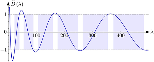
Figure 1. Plot of the approximate function $\tilde{D}(\lambda )$ for the Kronig-Penney model from Example 1.

TABLE 1

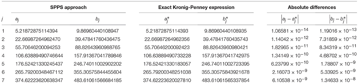
Table 1. Some spectral bands of the Kronig-Penney model calculated from the SPPS approach and the exact expression (28).

Example 2 (Potential without point interactions). Suppose that operator S_q has a potential q consisting on only the regular part q₀ defined by

$\begin{array}{ll}{q}_0(x)=-2-\text{sech}(x-2),0\le x<4,& (\mathrm{32a})\end{array}$

$\begin{array}{ll}{q}_0(x+4)=q_0(x),\forall x\in ℝ.& (\mathrm{32b})\end{array}$

It follows that n = 0, ℓ = 4, and ${{Y}}_0=\mathrm{\text{Ø}}$. Operator S_q0 defines an unbounded operator ${{H}}_{q_0}$ in L²(ℝ) with domain H²(ℝ). The transmission matrix is given by T = M_{0, 1}, where the monodromy matrix

${\text{M}}_{0,1}(\text{λ})=\left(\begin{array}{cc}{\varphi }_1(\ell ;\text{λ})& {\varphi }_2(\ell ;\text{λ})\\ {({\varphi }_1)}_x^{\prime }(\ell ;\text{λ})& {({\varphi }_2)}_x^{\prime }(\ell ;\text{λ})\end{array}\right)$

is defined from a pair of solutions ϕ₁, ϕ₂ of the equation S_q0u = λu, 0 < x < ℓ, satisfying the Cauchy conditions ϕ₁(0;λ) = 1, ${\varphi }_1^{\prime }(0;\lambda )=0$, ϕ₂(0;λ) = 0, ${\varphi }_2^{\prime }(0;\lambda )=1$. In this example the function $D(\lambda )=\frac{1}{2}({\varphi }_1(\ell ;\lambda )+{({\varphi }_2)}_x^{\prime }(\ell ;\lambda ))$ is approximated by the SPPS approach described in subsection 4.3. In Figure 2 we can see the plot of the approximate function $\tilde{D}(\lambda )$ and its intersections with the horizontal lines ±1 that define the spectral bands [a_j, b_j]. In Table 2 we observe some spectral bands of ${{H}}_{q_0}$, whose edges were calculated from the zeros of the equations $\tilde{D}(\lambda )\pm 1=0$. The fourth and fifth columns of the table show the widths of the bands and the gaps, respectively. We can see a monotonically increasing of the band widths, while the gaps monotonically decrease. Such a behavior is a characteristic of smooth periodic potentials (see, e.g., [31]) The considered potential q₀ is smooth except at a countable set of points of the form x_k = kℓ, k ∈ ℤ, nonetheless the potential is continuous at these points.

FIGURE 2

Figure 2. Plot of the approximate function $\tilde{D}(\lambda )$ from Example 2.

TABLE 2

Table 2. Some spectral bands [a_j, b_j] of the Hamiltonian ${{H}}_{q_0}$ from Example 2.

Example 3 (Potential including δ-interactions). Let the potential q of Schrödinger operator S_q be a π-periodic function defined by

$q(x)=q_0+{\displaystyle \sum _{n\in \mathbb{Z}}}2\delta \left(x+\left(n+\frac{1}{2}\right)\pi \right),$

where the regular potential is the piecewise continuous periodic function

$\begin{array}{ll}{q}_0(x)=\{\begin{array}{ll}\sin (2x)+1,\hfill & 0\le x<\pi /2,\hfill \\ -1,\hfill & \pi /2\le x<\pi ,\hfill \end{array}& (\mathrm{33a})\end{array}$

$\begin{array}{ll}{q}_0(x+\pi )=q_0(x),\forall x\in ℝ.& (\mathrm{33b})\end{array}$

It follows that n = 1, ℓ = π, and ${{Y}}_0=\left\{\pi /2\right\}$. The transmission matrix is given by T(λ) = M_{1, 2}(λ)A₁M_{0, 1}(λ), where

${\text{A}}_1=\left(\begin{array}{ll}1& 0\\ 2& 1\end{array}\right).$

The approximation of function $D(\lambda )=\frac{1}{2}(T_{11}(\lambda )+T_{22}(\lambda ))$ obtained by the SPPS approach is plotted in Figure 3. In Table 3 we observe some spectral bands of ${{H}}_{q_0}$, whose edges were calculated from the zeros of the equations $\tilde{D}(\lambda )\pm 1=0$. According to the fourth and fifth columns of the table we can see that both the band widths and gaps have a tendency to grow. Moreover, the band-to-gap ratio also has an exponential tendency to grow. This characteristic is shared by operators with singular potentials including point interactions (cf. [25]).

FIGURE 3

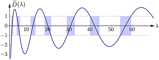
Figure 3. Plot of the approximate function $\tilde{D}(\lambda )$ from Example 3.

TABLE 3

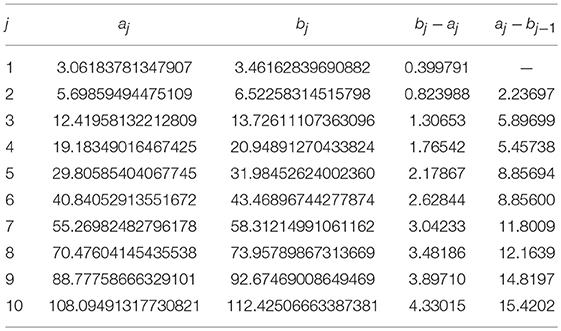
Table 3. Some spectral bands [a_j, b_j] of the Hamiltonian ${{H}}_{q_0}$ from Example 3.

Example 4 (Potential including δ′-interactions). Let us consider a periodic potential q involving δ′-interactions

$q(x)=q_0+{\displaystyle \sum _{n\in \mathbb{Z}}}\left({\delta }^{\prime }\left(x+n+\frac{1}{4}\right)+2{\delta }^{\prime }\left(x+n+\frac{1}{2}\right)\right),$

where the regular potential is defined by

$\begin{array}{ll}{q}_0(x)=4x-2,q_0(x+1)=q_0(x),\forall x\in ℝ.& (34)\end{array}$

In this example n = 2, ℓ = 1, and ${{Y}}_0=\left\{\frac{1}{4},\frac{1}{2}\right\}$. The transmission matrix is given by

$\begin{array}{ll}\text{T}(\text{λ})={\text{M}}_{2,3}(\text{λ}){\text{A}}_2{\text{M}}_{1,2}(\text{λ}){\text{A}}_1{\text{M}}_{0,1}(\text{λ}),& (35)\end{array}$

where

${\text{A}}_1=\left(\begin{array}{cc}1& -1\\ 0& 1\end{array}\right),{\text{A}}_2=\left(\begin{array}{cc}1& -2\\ 0& 1\end{array}\right).$

The approximate function $\tilde{D}(\lambda )$ obtained from the SPPS approach is plotted in Figure 4. In this case the spectral bands are indicated by thin vertical strips in the plot. In Table 4 we observe some spectral bands of ${{H}}_{q_0}$ calculated from the zeros of the equations $\tilde{D}(\lambda )\pm 1=0$. The table shows a narrowness of the bands compared with the large gaps, which can be understood on the fact that at the high values of λ the unit cells of the periodic problem get decoupled since δ′-interaction approximates to Neumann conditions [25, 26]. We also observe that the peaks of the plot of $\tilde{D}$ are dominated by a straight line with positive slope, which accounts for the increasing gaps of the spectrum. The considered problem has spectral properties that resemble those of Wannier-Stark ladders for a periodic array of δ′-scatterers [26]. These observations agree with the spectra of systems with periodically distributed δ′-distributions (see, e.g., [22, 27, 28]).

FIGURE 4

Figure 4. Plot of the approximate function $\tilde{D}(\lambda )$ from Example 4.

TABLE 4

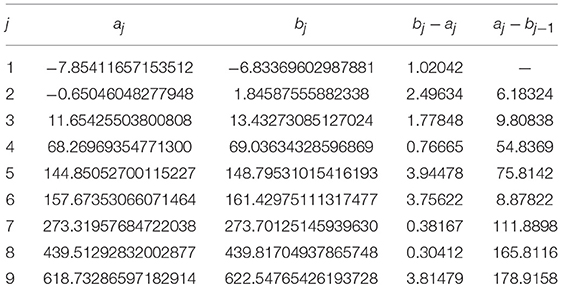
Table 4. Some spectral bands [a_j, b_j] of the Hamiltonian ${{H}}_{q_0}$ from Example 4.

Example 5 (Potential including both δ- and δ′-interactions). In this example we consider the following periodic potential

$q(x)=q_0+{\displaystyle \sum _{n\in \mathbb{Z}}}\left(2\delta \left(x+n+\frac{1}{4}\right)-2{\delta }^{\prime }\left(x+n+\frac{3}{4}\right)\right),$

which involves both δ- and δ′-interactions, where the regular potential is given by

$q_0(x)=10{\left(x-\frac{1}{2}\right)}^2,q_0(x+1)=q_0(x),\forall x\in ℝ.$

In this case n = 2, ℓ = 1, ${{Y}}_0=\left\{\frac{1}{4},\frac{3}{4}\right\}$, and the transmission matrix is given by expression (37), where the matrices

${\text{A}}_1=\left(\begin{array}{cc}1& 0\\ 2& 1\end{array}\right),{\text{A}}_2=\left(\begin{array}{cc}1& 2\\ 0& 1\end{array}\right).$

On applying the SPPS approach we calculate the approximate function $\tilde{D}(\lambda )$, which is shown in Figure 5. From the zeros of the equations $\tilde{D}(\lambda )\pm 1=0$ we obtain the spectral bands of ${{H}}_{q_0}$, which are shown in Table 5. The spectrum of this operator shares common characteristics with the previous spectra, for instance, the large gap-to-band ratio due to the presence of δ- and δ′-interactions.

FIGURE 5

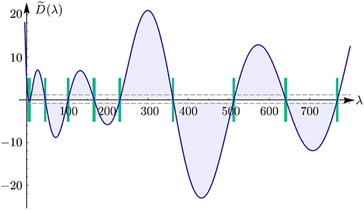
Figure 5. Plot of the approximate function $\tilde{D}(\lambda )$ from Example 5.

TABLE 5

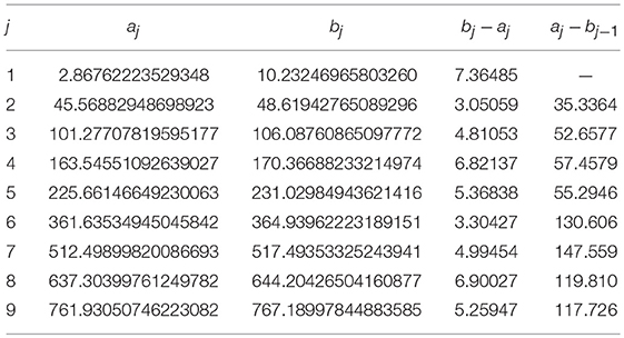
Table 5. Some spectral bands [a_j, b_j] of the Hamiltonian ${{H}}_{q_0}$ from Example 5.

Previous examples show the applicability of the SPPS method in the numerical determination of the spectral bands of periodic Schrödinger operators with point interactions. For numerically simulating the influence of a slowly oscillating at infinity potential q₁ on the gaps of the essential spectrum of the operators it is necessary to determine the numbers $m_{q_1}^{\infty }$ and $M_{q_1}^{\infty }$, and employ formula (19) for calculating the essential spectrum of the perturbed operator.

Example 6 (Perturbed periodic potential). Let $q_1(x)=Asin|x{|}^{\epsilon }$, ε ∈ (0, 1), A > 0, x ∈ ℝ. Since q₁ ∈ SO (ℝ), it is easy to see that for every sequence ℝ∋ h_m → ∞ the limit $q_1^h$ is a real constant. The limiting values satisfy $\left|q_1^h\right|\le A$ for every real sequence h = {h_m}, hence, $m_{q_1}^{\infty }=-A$ and $M_{q_1}^{\infty }=A$.

Let us consider the previous Example 2 and suppose that its regular potential q₀ defined in (34) is perturbed by the potential q₁ ∈ SO (ℝ) with A = 1. In Table 6 we observe the influence of this slowly oscillating function on the spectrum of the unperturbed operator ${{H}}_{q_0}$. We observe the broadening of the bands and their corresponding overlapping when the gaps are negative. Since the gaps of the unperturbed problems are monotonically decreasing all the bands will overlap producing a continuous spectrum

$\text{s}{\text{p}}_{\text{ess}}{{H}}_{q_0+q_1}=\left[a_1+m_{q_1}^{\infty },+\infty \right)=\left[-3.67428666671436,+\infty \right).$

TABLE 6

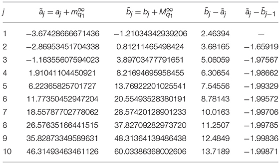
Table 6. Some spectral bands [a_j, b_j] of the perturbed Hamiltonian ${{H}}_{q_0+q_1}$ from Example 2.

Now, let us consider the previous Example 3, and suppose that its regular potential q₀ defined in (35) is perturbed by a more intense perturbation q₁∈SO(ℝ) with A = 6. The bands of the resulting perturbed operator ${{H}}_{q_0+q_1}$ are shown in Table 7. In this case the first seven bands of the spectrum overlap, yielding the merged band

$\begin{array}{l}\left[a_1+m_{q_1}^{\infty },b_7+M_{q_1}^{\infty }\right]=\left[-2.93816218652093,64.31214991061162\right]\\ \subset \text{s}{\text{p}}_{\text{ess}}{{H}}_{q_0+q_1}.\end{array}$

TABLE 7

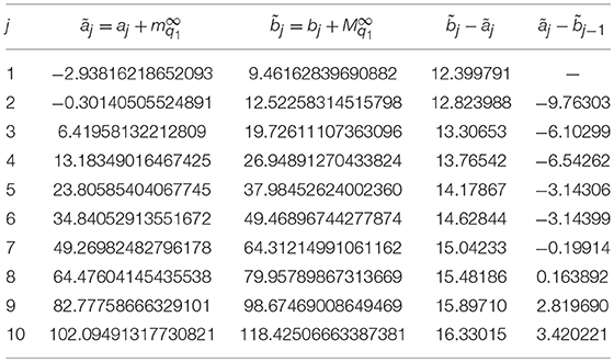
Table 7. Some spectral bands [a_j, b_j] of the perturbed Hamiltonian ${{H}}_{q_0+q_1}$ from Example 3.

From the eighth band, the gaps of the spectrum are open. Hence, in order to close more gaps, it is necessary to increase the intensity of the perturbation.

Finally, on considering the potential (36) from Example 4 and the perturbation q₁ ∈ SO (ℝ) with A = 3 we obtain the spectral bands shown in Table 8. In this case, though the bands get broader, none of them overlap with the given perturbation.

TABLE 8

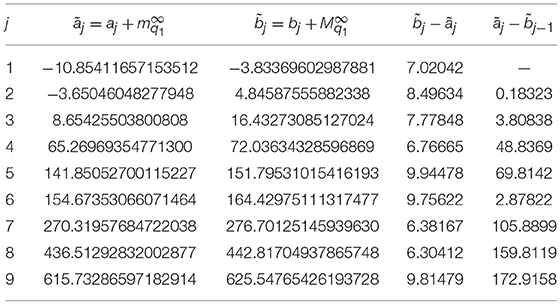
Table 8. Some spectral bands [a_j, b_j] of the perturbed Hamiltonian ${{H}}_{q_0+q_1}$ from Example 4.

6. Conclusions

In this work we have approached one-dimensional Schrödinger operators with point interactions from their corresponding self-adjoint extensions. On assuming that the point interactions are supported on an infinite countable set with a periodic structure we were able to employ the limit operators method for analyzing their essential spectra. If the regular potentials are periodic the Floquet-Bloch theory leads to a formula defining the band-gap spectra of the periodic operators, which is given in terms of a function D(λ). This function is obtained from the monodromy matrices specified at the points where the singular potential is supported. In this work the function D(λ) is determined by the SPPS method, which allows to consider arbitrary regular potentials q₀ satisfying certain smoothness conditions, and to derive numerical methods for calculating the band edges of spectra of periodic problems involving point interactions.

We also considered the case when periodic problems are perturbed by slowly oscillating at infinity terms, which can model impurities in the crystals. The perturbed problems are also approached by the limit operators method, which gives a neat formula for their essential spectra. The spectral analysis of perturbed periodic problems relies on a pair of numbers $m_{q_1}^{\infty }$ and $M_{q_1}^{\infty }$ that depend on the perturbation q₁ ∈ SO(ℝ) specified in the problem. These numbers, in general, lead to the broadening (narrowing) of the bands (gaps), which may change significantly the spectra of the operators. The SPPS approach together with the determination of the numbers $m_{q_1}^{\infty }$, $M_{q_1}^{\infty }$ give a simpler way for determining the spectra of perturbed periodic problems.

The applicability of the SPPS method and the limit operators method is shown by the numerical examples considered in this work that involved δ- and δ′-interactions as well as a periodic regular potential q₀. The accuracy of the results relies on the uniform convergence of power series of the spectral parameter that define the solutions of the involved Schrödinger equations, so that an increasingly number N of terms in the truncated series will reduce the associated errors in the numerical values. Finally, the theory developed in this work can be used for analyzing photonic crystals and electromagnetic waveguides with periodic refractive profiles, as well as quantum problems involving periodic potentials.

Data Availability

All datasets generated and analyzed for this study are included in the manuscript and the supplementary files.

Author Contributions

VR conceived the idea of the paper and developed the theoretical formalism. VB-F performed the analytic calculations, designed the examples, and analyzed the numerical data. VR, VB-F, and LO contributed to the final version of the manuscript.

Funding

VB-F acknowledges CONACyT for support via grant 283133.

Conflict of Interest Statement

The authors declare that the research was conducted in the absence of any commercial or financial relationships that could be construed as a potential conflict of interest.

References

1. Kronig RdeL. The quantum theory of dispersion in metallic conductors. Proc R Soc Lond A. (1929) 124:409–22. doi: 10.1098/rspa.1929.0125

CrossRef Full Text | Google Scholar

2. Kronig RdeL, Penney WG. Quantum mechanics of electrons in crystal lattices. Proc R Soc Lond A. (1931) 130:499–513. doi: 10.1098/rspa.1931.0019

CrossRef Full Text | Google Scholar

3. Albeverio S, Kurasov P. Singular Perturbations of Differential Operators. Solvable Schrodinger Type Operators. Cambridge: Cambridge University Press (2000). p. 429.

4. Albeverio S, Gesztesy F, Høegh-Krohn R, Holden H. Solvable Models in Quantum Mechanics. 2nd edn. Providence, RI: AMS Chelsea Publishing (2004). p. 488.

5. Berezin FA, Faddeev LD. A remark on Schrödinger operators with a singular potentials. Soviet Math Dokl. (1961) 2:372–5.

6. Gadella M, Negro J, Nieto L M. Bound states and scattering coefficients of the −aδ(x)+bδ′(x) potential. Phys Lett A. (2009) 373:1310–3. doi: 10.1016/j.physleta.2009.02.025

CrossRef Full Text | Google Scholar

7. Kostenko AS, Malamud MM. One-dimensional Schrödinger operator with δ-interactions. Funct Anal Appl. (2010) 44:151–5. doi: 10.1007/s10688-010-0019-9

CrossRef Full Text | Google Scholar

8. Kurasov P. Distribution theory for discontinuous test functions and differential operators with generalized coefficients. J Math Anal Appl. (1996) 201:297–323. doi: 10.1006/jmaa.1996.0256

CrossRef Full Text | Google Scholar

9. Kurasov P, Larson J. Spectral asymptotics for Schrödinger operators with periodic point interactions. J Math Anal Appl. (2002) 266:127–48. doi: 10.1006/jmaa.2001.7716

CrossRef Full Text | Google Scholar

10. Kravchenko VV, Porter MR. Spectral parameter power series for Sturm-Liouville problems. Math Meth Appl Sci. (2010) 33:459–68. doi: 10.1002/mma.1205

CrossRef Full Text | Google Scholar

11. Golovaty Y. 1D Schrödinger operators with short range interactions: two-scale regularization of distributional potentials. Integr Equat Oper Theor. (2013) 75:341–62. doi: 10.1007/s00020-012-2027-z

CrossRef Full Text | Google Scholar

12. Golovaty YD, Hryniv RO. Norm resolvent convergence of singularly scaled Schrödinger operators and δ′-potentials. Proc R Soc Edinb A. (2013) 143:791–816. doi: 10.1017/S0308210512000194

CrossRef Full Text | Google Scholar

13. Golovaty Y. Schrödinger operators with singular rank-two perturbations and point interactions. Integr Equat Oper Theor. (2018) 90:57. doi: 10.1007/s00020-018-2482-2

CrossRef Full Text | Google Scholar

14. Agranovich MS. Elliptic boundary problems. In: Agranovich MS, Egorov YuV, Shubin MA (eds.). Partial Differential Equations IX, Elliptic Boundary Value Problems. Berlin: Springer (1997). p. 1–144.

Google Scholar

15. Rabinovich VS. Elliptic differential operators on infinite graphs with general conditions on vertices. Complex Var Ellipt. (2019). (In press) doi: 10.1080/17476933.2019.1575824

CrossRef Full Text | Google Scholar

16. Agranovich MS, Vishik MI. Elliptic problems with a parameter and parabolic problems of general type. Russ Math Surv. (1964) 19:53. doi: 10.1070/RM1964v019n03ABEH001149

CrossRef Full Text | Google Scholar

17. Rabinovich VS. Essential spectrum of Schrödinger operators on periodic graphs. Funct Anal Appl. (2018) 52:66–9. (Translated from Funktsional Anal Prilozhen. (2018) 52:80–84.) doi: 10.1007/s10688-018-0210-y

CrossRef Full Text | Google Scholar

18. Birman MSh, Solomjak MZ. Spectral Theory of Self-Adjoint Operators in Hilbert Space. Dordrecht: Reidel Publishing Company (1987). p. 301.

19. Rabinovich VS, Roch S, Silbermann B. Limit Operators and Their Applications in Operator Theory. Basel: Birkhäuser (2004). p. 392.

20. Lindner M, Seidel M. An affirmative answer to a core issue on limit operators. J Funct Anal. (2014) 267:901–17. doi: 10.1016/j.jfa.2014.03.002

CrossRef Full Text | Google Scholar

21. Kuchment P. An overview of periodic elliptic operators. Bull Amer Math Soc. (2016) 53:343–414. doi: 10.1090/bull/1528

CrossRef Full Text | Google Scholar

22. Barseghyan D, Khrabustovskyi A. Gaps in the spectrum of a periodic quantum graph with periodically distributed δ′-type interactions. J Phys A Math Theor. (2015) 48:255201. doi: 10.1088/1751-8113/48/25/255201

CrossRef Full Text | Google Scholar

23. Cheon T, Shigehara T. Realizing discontinuous wave functions with renormalized short-range potentials. Phys Lett A. (1998) 243:111-6. doi: 10.1016/S0375-9601(98)00188-1

CrossRef Full Text | Google Scholar

24. Seba P. Some remarks on the δ′-interaction in one dimension. Rep Math Phys. (1986) 24:111–20. doi: 10.1016/0034-4877(86)90045-5

CrossRef Full Text | Google Scholar

25. Avron JE, Exner P, Last Y. Periodic Schrödinger operators with large gaps and Wannier–Stark ladders. Phys Rev Lett. (1994) 72:896. doi: 10.1103/PhysRevLett.72.896

PubMed Abstract | CrossRef Full Text | Google Scholar

26. Exner P. The absence of the absolutely continuous spectrum for δ′ Wannier-Stark ladders. J Math Phys. (1995) 36:4561–70. doi: 10.1063/1.530908

CrossRef Full Text | Google Scholar

27. Exner P, Neidhardt H, Zagrebnov V. Potential approximations to δ′: an inverse Klauder phenomenon with norm-resolvent convergence. Commun Math Phys. (2001) 224:593–612. doi: 10.1007/s002200100567

CrossRef Full Text | Google Scholar

28. Maioli M, Sacchetti A. Absence of absolutely continuous spectrum for Stark-Bloch operators with strongly singular periodic potentials. J Phys A. (1995) 28:1101. (Erratum (1998) A31:1115. doi: 10.1088/0305-4470/31/3/024)

CrossRef Full Text | Google Scholar

29. Wannier GH. Wave functions and effective Hamiltonian for Bloch electrons in an electric field. Phys Rev. (1960) 117:432. doi: 10.1103/PhysRev.117.432

CrossRef Full Text | Google Scholar

30. Kravchenko VV. A representation for solutions of the Sturm–Liouville equation. Complex Var Ellipt. (2008) 53:775–89. doi: 10.1080/17476930802102894

CrossRef Full Text | Google Scholar

31. Weinstein MI, Keller JB. Asymptotic behavior of stability regions for Hill's equation. SIAM J Appl Math. (1987) 47:941–58. doi: 10.1137/0147062

CrossRef Full Text | Google Scholar