A Note on Capon's Minimum Variance Projection for Multi-Spacecraft Data Analysis

Capon's minimum variance projection for the multi-point measurements is revisited using the method of likelihood function to derive the minimum variance projection and a simplified error estimate analytically. Theoretical construction of the minimum variance projection assumes a Gaussian form of the likelihood function and also regards the data covariance as a proxy of the noise covariance. The minimum variance projection is extended to the problem of two-spacecraft mode decomposition in the Mercury magnetosphere in which the magnetic field is a superposition of the constant field from the current sheet and the dipolar field from the planet. The extension of the Capon estimator (the data-variance projection) can identify the signal amplitudes of the different fields with a sufficient accuracy when the statistical averaging is properly done. The Capon estimator serves as a powerful analysis tool when the spatial resolution is limited to only a few points.

1. Capon's Minimum Variance Projection

Minimum variance projection introduced by Capon [1] has a wide range of applications in the geophysical and space physical research fields whenever multi-point measurements are available.

Various formations are possible in the multi-point measurements (Figure 1): the THEMIS mission in a one-dimensional array aligned with a magnetic field line [2], the Swarm mission spanning a plane with three spacecraft [3, 4], and the Cluster mission [5] the MMS mission [6] forming a tetrahedron.

FIGURE 1

Figure 1. Multi-point spacecraft configurations.

The projection works with various kinds of shape vectors (or models for the data) by minimizing the projection error without changing the amplitude of the signal amplitude. The minimum variance projection is, after Capon [1] or Haykin [7], obtained by imposing a constrained optimization:

$\begin{array}{ll}\text{minimize }\overrightarrow{w}\text{R}\overrightarrow{w}\text{ subject to }\overrightarrow{w}\overrightarrow{h}=1,& (1)\end{array}$

or, by formulating into a variational problem using the variation operator δ[⋯ ] and the Lagrangian multiplier λ,

$\begin{array}{ll}\delta \left[\overrightarrow{w}\text{R}\overrightarrow{w}-\lambda \left(\overrightarrow{w}\overrightarrow{h}-1\right)\right]=0.& (2)\end{array}$

Here $\overrightarrow{w}$ is the weight vector operating on the measurement covariance matrix $\text{R}=\langle \overrightarrow{d}\overrightarrow{d}\rangle$, $\overrightarrow{d}$ the measurement data in a vectorial form, 〈⋯ 〉 the operation of ensemble averaging, $\overrightarrow{h}$ the shape vector. The problem (Equation 2) can analytically be solved. The solution is, blue by treating the shape vector as a complex-number vector,

$\begin{array}{ll}\overrightarrow{w}=\frac{{\text{R}}^{-1}\overrightarrow{h}}{{\overrightarrow{h}}^{†}{\text{R}}^{-1}\overrightarrow{h}}.& (3)\end{array}$

See, for example, Haykin [7] for the derivation. The projected power (squared signal amplitude) is

$\begin{array}{ll}P={\overrightarrow{w}}^{†}\text{R}\overrightarrow{w}={\left[{\overrightarrow{h}}^{†}{\text{R}}^{-1}\overrightarrow{h}\right]}^{-1}.& (4)\end{array}$

A larger set of algorithms has so far been developed in the frame of direction-of-arrival estimation in the adaptive filter theory. Many algorithms are recently reviewed by Khmou et al. [8], including beamforming method, Bartlett method, Capon method, linear prediction method, maximum entropy method, Pisarenko harmonic decomposition, minimum norm, MUSIC algorithm, propagator method, and partial covariance matrix method. In the multi-spacecraft wave-field analysis, three methods are most relevant: beamforming method, Capon method, and MSR method [9].

• The beamforming method can easily be implemented to the data analysis, but on the other hand provides a lower resolution of the signal-to-noise ratio in the spectral analysis compared to the Capon method when only few data points are used in the analysis [10, 11]

• The Capon method is versatile in the multi-spacecraft data analysis because the method can be extended in various ways, e.g., to the vectorial data set (the wave telescope technique) [12, 13] to different field types (e.g., electric field and magnetic field used in the k-filtering technique) [14], and to the mode decomposition (this paper).

• The MSR method [11] uses both the Capon (or the wave telescope) method and the eigenvector-based method (the extended MUSIC algorithm), and provides an improved signal-to-noise ratio in the wavevector spectrum. The MSR method is optimized in the estimate of the total fluctuation energy (i.e., trace of the spectral density matrix) but not to the matrix elements. Also, the MSR method is constrained to the isotropic noise assumption.

So far, three shape vectors for the Capon method have successfully been applied to the multi-spacecraft data analysis blue in the field of space physics

1. Plane waves [1, 12, 14]:

$\begin{array}{ll}{h}_i(k_{\text{x}},k_{\text{y}},k_{\text{z}})=exp\left[\text{i}\left(k_{\text{x}}{r}_{\text{x}i}+k_{\text{y}}{r}_{\text{y}i}+k_{\text{z}}{r}_{\text{z}i}\right)\right],& (5)\end{array}$

where {k_x, k_y, k_z} are the three components of the wavevectors, {r_xi, r_yi, r_zi} the spatial coordinates of the i-th sensor, and i the imaginary number unit.

2. Spherical waves [15, 16]:

$\begin{array}{ll}{h}_i(k,r_{\text{xc}},r_{\text{yc}},r_{\text{zc}})={\left[{\displaystyle \sum _{i=1}^n}\frac{1}{|{\overrightarrow{r}}_i-{\overrightarrow{r}}_{\text{c}}{|}^2}\right]}^{-1/2}\frac{exp\left[\text{i}k|{\overrightarrow{r}}_i-{\overrightarrow{r}}_{\text{c}}|\right]}{|{\overrightarrow{r}}_i-{\overrightarrow{r}}_{\text{c}}|},& (6)\end{array}$

where k is the wavenumber, and ${\overrightarrow{r}}_{\text{c}}=\left[r_{\text{xc}},r_{\text{yc}},r_{\text{zc}}\right]$ the coordinate of the spherical wave center. The summation in the normalization constant runs over the number of sensors n.

3. Phase-shifted waves [17]:

$\begin{array}{ll}{h}_i(\text{Φ},r_{\text{xc}},\text{Δ}x,k_{\text{y}})=exp\left[\text{i}\left(\Phi \text{ arctan}\left(\frac{r_{\text{x}i}-r_{\text{xc}}}{\text{Δ}x}\right)+k_{\text{y}}{r}_{\text{y}i}\right)\right],& (7)\end{array}$

where Φ is the amount of phase jump, r_xc the x-coordinate of the phase jump center, Δx the x-width (or range in x) of the phase jump around the center, and k_y the y-component of the wavenumber.

Capon's minimum variance projection uses the measurement data to guide the projection by minimizing the estimated power during the projection (in spirit of minimizing uncertainty) yet keeping the gain. We address the question here, “Why is the inversion of the data covariance matrix R⁻¹ used in the Capon projection (Equation 3) and in the spectrum (Equation 4)?” In this paper, we offer an answer to this question, that is, the Capon method uses the measured data as a proxy of the noise property upon the optimization procedure. The method of the likelihood function is introduced to give an alternative and more instinctive derivation of Capon's method. Moreover, by revisiting Capon's minimum variance projection through the likelihood function method, it becomes clear that one may project the measurement data not only onto a single shape vector but also onto a multitude of shape vectors, which will enhance the capability of the multi-spacecraft data analysis.

It is worthwhile to note that the maximum likelihood and the minimum variance aspects of the Capon estimator are already covered in detail in the original paper by Capon et al. [18] for a seismic array problem. In this paper, the essence of the Capon estimator is reviewed (in section 2) and the estimator is extended to the problem of mode decomposition. As an application, a new method is constructed (in section 3) for two-spacecraft measurements in the magnetosphere to identify the magnetic field of the current sheet origin and the dipolar field from the planet, which is relevant to the BepiColombo mission.

2. A View From Likelihood Function

2.1. Scalar Field

Minimum variance projection can be formulated using the likelihood function ${L}$ as follows (see also [19]). Consider a model for the observational data as

$\begin{array}{ll}{d}_i=h_{i}s+{\eta }_i,& (8)\end{array}$

where d_i is the data element at the i-th sensor (i = {1, 2, ⋯ , n}, so n is the number of sensors), h_i the shape vector given a priori as a model, s the signal (in which we are interested), and η_i the noise at the i-th sensor. The noise is characterized by the n × n noise matrix N

$\begin{array}{ll}{N}_{ij}=\langle {\eta }_i{\eta }_j\rangle .& (9)\end{array}$

Again, the angular bracket 〈⋯ 〉 denotes the ensemble averaging over different realizations. The averaging is important because otherwise the determinant of the matrix vanishes and the matrix cannot be inverted.

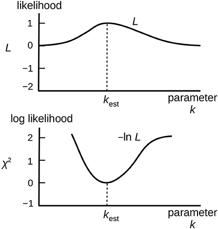
We minimize the squared deviation between the model and the data, i.e., we minimize χ² constructed (Figure 2) because of the steeper gradient toward the minimum (or the extremum) than that of the Gaussian curve as follows,

$\begin{array}{ll}{\chi }^2=\langle {\displaystyle \sum _{j=1}^n}{\displaystyle \sum _{i=1}^n}(d_i-h_{i}s)N_{ij}^{-1}(d_j-h_{j}s)\rangle & (10)\end{array}$

with respect to the signal s. We now assume a Gaussian shape for the likelihood function,

$\begin{array}{ll}{L}\propto exp\left[-\frac{{\chi }^2}{2}\right].& (11)\end{array}$

The likelihood function ${L}$ represents the probability of finding the true signal value for s under the given data set d_i.

FIGURE 2

Figure 2. Likelihood function on linear and logarithmic scales. Likelihood function is approximated to a Gaussian curve around the maximum (or the minimum of ${\chi }^2=-ln{L}$ in the parameter space k.

Our goal is to estimate the signal amplitude (denoted as $\tilde{s}$) for the shape vector for the given data set by finding a maximum of the likelihood function or equivalently by minimizing the deviation χ².

We differentiate χ² with respect to the signal s,

$\begin{array}{ll}\frac{\partial {\chi }^2}{\partial s}=-2\langle {\displaystyle \sum _{i=1}^n}{\displaystyle \sum _{j=1}^n}{h}_i{N}_{ij}^{-1}(d_j-h_{j}s)\rangle .& (12)\end{array}$

Requiring that the derivative be zero (which corresponds to the extremum), ∂(χ²)/∂s, we obtain

$\begin{array}{ll}\langle {\displaystyle \sum _{i=1}^n}{\displaystyle \sum _{j=1}^n}{h}_i{N}_{ij}^{-1}(d_j-h_{j}s)\rangle =0.& (13)\end{array}$

Equation (13) can be arranged into the following form,

$\begin{array}{ll}\langle {\displaystyle \sum _{i=1}^n}{\displaystyle \sum _{j=1}^n}{h}_i{N}_{ij}^{-1}{h}_{j}s\rangle =\langle {\displaystyle \sum _{i=1}^n}{\displaystyle \sum _{j=1}^n}{h}_i{N}_{ij}^{-1}{d}_j\rangle .& (14)\end{array}$

Note that the part in the angular bracket on the left hand side of Equation (14) is already statistically evaluated, so one may leave the angular bracket out in the following discussion. For a scalar quantity of s, one may obtain the estimator $\tilde{s}$ as

$\begin{array}{ll}\tilde{s}={\left[{\displaystyle \sum _{i=1}^n}{\displaystyle \sum _{j=1}^n}{h}_i{N}_{ij}^{-1}{h}_j\right]}^{-1}\langle {\displaystyle \sum _{i=1}^n}{\displaystyle \sum _{j=1}^n}{h}_i{N}_{ij}^{-1}{d}_j\rangle & (15)\end{array}$

$\begin{array}{lll}=& C_{\text{N}}\langle {\displaystyle \sum _{i=1}^n}{\displaystyle \sum _{j=1}^n}{h}_i{N}_{ij}^{-1}{d}_j\rangle ,& (16)\end{array}$

where C_N is the noise covariance,

$\begin{array}{ll}{C}_{\text{N}}={\left[{\displaystyle \sum _{i=1}^n}{\displaystyle \sum _{j=1}^n}{h}_i{N}_{ij}^{-1}{h}_j\right]}^{-1}.& (17)\end{array}$

Or, in a matrix notation,

$\begin{array}{ll}\tilde{s}=C_{\text{N}}\langle \overrightarrow{h}{\text{N}}^{-1}\overrightarrow{d}\rangle & (18)\end{array}$

and

$\begin{array}{ll}{C}_{\text{N}}={(\text{h}{\text{N}}^{-1}\text{h})}^{-1}& (19)\end{array}$

The signal covariance (or the optimized power estimate) is (by noting that the ensemble averaging is taken after the covariance calculation)

$\begin{array}{ll}{C}_{\text{R}}=\langle \tilde{s}\tilde{s}\rangle & (20)\end{array}$

$\begin{array}{lll}=& \langle C_{\text{N}}\overrightarrow{h}{\text{N}}^{-1}\overrightarrow{d}\overrightarrow{d}({\text{N}}^{-1})\overrightarrow{h}{C}_{\text{N}}\rangle & (21)\end{array}$

$\begin{array}{lll}=& C_{\text{N}}\overrightarrow{h}{\text{N}}^{-1}\langle \overrightarrow{d}\overrightarrow{d}\rangle ({\text{N}}^{-1})\overrightarrow{h}{C}_{\text{N}}.& (22)\end{array}$

In general, the data covariance matrix $\text{R}=\langle \overrightarrow{d}\overrightarrow{d}\rangle$ and the noise covariance matrix N must be evaluated separately, or the noise covariance matrix needs to be known a priori to determine the signal covariance C_S. Capon's minimum variance projection is obtained by imposing (or using) the data covariance matrix as the noise covariance matrix, N → R. An explicit calculation yields

$\begin{array}{ll}{C}_{\text{R}}=C_{\text{N}}\overrightarrow{h}{\text{R}}^{-1}\overrightarrow{h}{C}_{\text{N}}& (23)\end{array}$

$\begin{array}{lll}=& {\left(\overrightarrow{h}{\text{R}}^{-1}\overrightarrow{h}\right)}^{-1}\overrightarrow{h}{\text{R}}^{-1}\overrightarrow{h}{\left(\overrightarrow{h}{\text{R}}^{-1}\overrightarrow{h}\right)}^{-1}& (24)\end{array}$

$\begin{array}{lll}=& {\left(\overrightarrow{h}{\text{R}}^{-1}\overrightarrow{h}\right)}^{-1}& (25)\end{array}$

2.2. Vector Field

The method with the likelihood function can be extended to the vector field treatment in a straightforward fashion. We construct the data model as follows.

$\begin{array}{ll}\overrightarrow{d}=\text{H}\overrightarrow{s}+\text{η}.& (26)\end{array}$

The data are arranged into a long vector, $\overrightarrow{d}=\left[d_{\text{x}1},d_{\text{y}1},d_{\text{z}1},d_{\text{x}2},d_{\text{y}2},d_{\text{z}2},\cdots d_{\text{z}N}\right]$. The signal amplitude vector is $\overrightarrow{s}=\left[s_{\text{x}},s_{\text{y}},s_{\text{z}}\right]$. H is the shape-and-pointing matrix.

$\begin{array}{ll}\text{H}=\left[\begin{array}{ccc}{h}_{\text{x}1}& 0& 0\\ 0& h_{\text{y}1}& 0\\ 0& 0& h_{\text{z}1}\\ h_{\text{x}2}& 0& 0\\ 0& h_{\text{y}2}& 0\\ 0& 0& h_{\text{z}2}\\ & ⋮\\ 0& 0& h_{\text{z}N}\\ \end{array}\right].& (27)\end{array}$

η is the noise with the same construction as that of $\overrightarrow{d}$ (with 3 × n elements). The essential difference from the scalar-field treatment is that the covariance becomes a matrix, e.g., ${\text{C}}_{\text{S}}=\langle \overrightarrow{s}\overrightarrow{s}\rangle$ for the signal covariance matrix. Repeating the same procedure (by taking care of the vector and matrix operations), the signal estimator for the m-th component (k = {x, y, z}) is obtained as

$\begin{array}{ll}{\tilde{s}}_k={\displaystyle \sum _{\ell }^{\text{x},\text{y},\text{z}}}{\displaystyle \sum _{i=1}^n}{\displaystyle \sum _{j=1}^n}{({\text{C}}_{\text{N}})}_{\ell k}{H}_{i\ell }{N}_{ij}^{-1}{d}_j,& (28)\end{array}$

where the summation on ℓ runs over the x, y, and z components, and that on i and j over the number of sensors. The signal estimator is given in a matrix notation as

$\begin{array}{ll}\tilde{\overrightarrow{s}}={\text{C}}_{\text{N}}\langle \text{H}{\text{N}}^{-1}\overrightarrow{d}\rangle & (29)\end{array}$

The noise covariance matrix C_N is given by

$\begin{array}{ll}{({\text{C}}_{\text{N}}^{-1})}_{\ell k}={\displaystyle \sum _{i=1}^n}{\displaystyle \sum _{j=1}^n}{H}_{i\ell }{N}_{ij}^{-1}{H}_{jk}& (30)\end{array}$

or, in a matrix notation,

$\begin{array}{ll}{\text{C}}_{\text{N}}={\left[\text{H}{\text{N}}^{-1}\text{H}\right]}^{-1}.& (31)\end{array}$

The signal covariance matrix, when using the data covariance matrix again as the noise covariance matrix, is

$\begin{array}{ll}{\text{C}}_{\text{R}}^{(\text{vec})}={\text{C}}_{\text{N}}\text{H}{\text{N}}^{-1}\text{R}{({\text{N}}^{-1})}^t\text{H}{\text{C}}_{\text{N}}& (32)\end{array}$

$\begin{array}{lll}\to & {\left[\text{H}{\text{R}}^{-1}\text{H}\right]}^{-1}.& (33)\end{array}$

2.3. Mode Decomposition

The minimum variance projection can be extended to multiple shape vectors. By doing so, it is possible to decompose the measurement data set into a spectrum of m different modes or shapes. We construct a model for the measurement data (scalar field) with a multitude of modes and a noise.

$\begin{array}{ll}{d}_i={\displaystyle \sum _{\alpha =1}^{\text{m}}}{h}_i^{\alpha }{s}^{\alpha }+{\eta }_i,& (34)\end{array}$

where d_i is the measured field at the i-th sensor, m the number of the modes introduced into the model, ${\overrightarrow{h}}^{\alpha }=\left\{{\overrightarrow{h}}^{(1)},{\overrightarrow{h}}^{(2)},\cdots ,{\overrightarrow{h}}^{(m)}\right\}$ is a set of shape vectors for modes α = {1, 2, ⋯ , m}, the symbol s^α is the signal amplitude at each mode, and n_i the noise at the i-th sensor.

Derivation of the minimum variance estimator is essentially the same as that for the single mode χ² minimization. The estimator for the signal amplitude at the α-th mode is obtained as

$\begin{array}{ll}{\tilde{s}}^{\alpha }=\langle {\displaystyle \sum _{\beta }^{\text{m}}}{\displaystyle \sum _{i=1}^n}{\displaystyle \sum _{j=1}^n}{({\text{C}}_{\text{N}})}^{\alpha \beta }{h}_i^{\beta }{N}_{ij}^{-1}{d}_j\rangle .& (35)\end{array}$

The noise covariance matrix is a projection of the inverse noise matrix N⁻¹ onto different modes (h^α and h^β),

$\begin{array}{ll}{({\text{C}}_{\text{N}}^{-1})}^{\alpha \beta }={\displaystyle \sum _{i=1}^n}{\displaystyle \sum _{j=1}^n}{h}_i^{(\alpha )}{N}_{ij}^{-1}{h}_j^{\beta }.& (36)\end{array}$

The signal covariance matrix for the Capon-type projection is obtained as

$\begin{array}{ll}{(\text{C})}^{\alpha \beta }={\text{C}}_{\text{N}}{\overrightarrow{h}}^{\alpha }{\text{N}}^{-1}\text{R}{\text{N}}^{-1}{\overrightarrow{h}}^{\beta }{\text{C}}_N& (37)\end{array}$

$\begin{array}{lll}\to & {\left[\overrightarrow{h^{\alpha }}{\text{R}}^{-1}{\overrightarrow{h}}^{\beta }\right]}^{-1}.& (38)\end{array}$

The diagonal elements in the signal covariance matrix are the power (squared signal amplitude) of each mode.

2.4. Error Estimate

A useful form for the one-sigma error (68 % confidence) for the minimum variance estimator can be evaluated from the likelihood function. Ideally, the inverse of the noise matrix N⁻¹ must be known, but the error estimate requires the knowledge on the noise property. Still, we obtain an insight by considering a special case, that is, we model the noise matrix N as diagonal with a value of each diagonal element C_S+C_N (which is a scalar). The likelihood function for a simplified error estimate is again modeled as Gaussian (see, e.g., Equation 11.21 in Dodelson [19]),

$\begin{array}{ll}{L}\propto \frac{1}{{(C_{\text{S}}+C_{\text{N}})}^{n/2}}exp\left[-\frac{1}{2}\frac{\langle {\displaystyle {\sum }_{i=1}^n}{(d_i-h_{i}s)}^2\rangle }{C_{\text{S}}+C_{\text{N}}}\right]& (39)\end{array}$

One-sigma error is obtained as the second-order derivative of the logarithm of the likelihood function (which is essentially χ² in the Gaussian likelihood model):

$\begin{array}{ll}{\sigma }_{\text{S}}={\left[-\frac{{\partial }^2}{\partial C_{\text{S}}^2}(ln{L})\right]}^{-1/2}& (40)\end{array}$

$\begin{array}{lll}=& \sqrt{\frac{2}{n}}(C_{\text{S}}+C_{\text{N}})& (41)\end{array}$

$\begin{array}{lll}\to & \sqrt{\frac{8C_{\text{S}}^2}{n}}.& (42)\end{array}$

Here Equation (40) is evaluated at the peak of the likelihood function to obtain (Equation 41), and the signal covariance C_S is used as a proxy of the noise covariance C_N for Capon's minimum variance projection in deriving (Equation 42). Thus, the simplified error of the Capon-estimated signal power is ${\sigma }^2=8C_{\text{S}}^2/n$. See Appendix for derivation of Equation (40).

3. Application

Mode decomposition using the minimum variance projection serves as a powerful analysis tool when the measurements are limited to only few spatial points. A test using a synthetic data set is presented with two-spacecraft measurements in the Mercury magnetosphere in view of the BepiColombo mission [20].

3.1. Setup

Magnetic fields are modeled as a superposition of two different fields (or modes), B^(a) and B^(b) and noise η in the magnetosphere at two sensor locations, r₁ = 480 km (planetary orbiter) and r₂ = 590 km (magnetospheric orbiter) above surface (at a radius of R_s = 2, 440 km for the planetary center). The measurement data are thus

$\begin{array}{ll}B(r_1)=B^{(\text{a})}(r_1)+B^{(\text{b})}(r_1)+{\eta }_1& (43)\end{array}$

$\begin{array}{ll}B(r_2)=B^{(\text{a})}(r_2)+B^{(\text{b})}(r_2)+{\eta }_2,& (44)\end{array}$

where the first mode is the magnetic field from the current sheet

$\begin{array}{ll}{B}^{(\text{a})}=s^{(\text{a})}=\text{const}.& (45)\end{array}$

and the second mode is the dipolar field from the planet

$\begin{array}{ll}{B}^{(\text{b})}=s^{(\text{b})}{\left(\frac{r}{R_{\text{s}}}\right)}^{-3}.& (46)\end{array}$

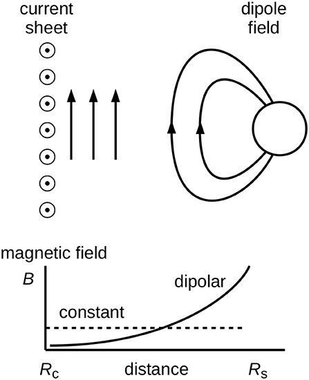
Measurements are assumed to be on the magnetic equatorial plane such that the magnetic fields have only one non-vanishing component (say, the z component). The geometrical configuration is illustrated in Figure 3. The true signal amplitudes are s^(a) = 20 nT and s^(b) = 200 nT, respectively. Noise is blue assumed to be Gaussian distributed with a standard deviation of σ_n = 1 nT. The goal of the numerical test using the synthetic data is to estimate the signal amplitudes for the two modes, ${\tilde{s}}^{(\text{a})}$ and ${\tilde{s}}^{(\text{b})}$ using the noise-variance minimization and the data-variance minimization.

FIGURE 3

Figure 3. Superposition of a constant field from the current sheet (mode 1) and a dipolar field from the planet (mode 2) in a region between the distance to the current sheet (from the planetary center) R_c and the that to the planetary surface R_s.

3.2. Analysis – Preparation

The shape vector for the first mode (a constant field) is

$\begin{array}{ll}{\overrightarrow{h}}_1=\left[\begin{array}{c}1\\ 1\end{array}\right]& (47)\end{array}$

and that for the second mode (decaying field) is

$\begin{array}{ll}{\overrightarrow{h}}_2=\left[\begin{array}{c}{\left(\frac{r_1}{R_{\text{s}}}\right)}^{-3}\\ {\left(\frac{r_2}{R_{\text{s}}}\right)}^{-3}\end{array}\right].& (48)\end{array}$

The shape matrix is constructed as $\left[{\overrightarrow{h}}_1{\overrightarrow{h}}_2\right]$,

$\begin{array}{ll}\text{h}=\left[\begin{array}{cc}1& {\left(\frac{r_1}{R_{\text{s}}}\right)}^{-3}\\ 1& {\left(\frac{r_2}{R_{\text{s}}}\right)}^{-3}\end{array}\right].& (49)\end{array}$

The data matrices are averaged over different realizations or samples,

$\begin{array}{ll}\text{R}=\langle \overrightarrow{d}\overrightarrow{d}\rangle ,& (50)\end{array}$

using an averaging size of N_s. The measurement data vector is averaged when using the minimum variance estimator as $\langle \overrightarrow{d}\rangle$. We study the minimum variance estimators for different sampling sizes N_s. The measurement noise matrix follows uncorrelated Gaussian statistics,

$\begin{array}{ll}\text{N}=\langle \overrightarrow{\eta }\overrightarrow{\eta }\rangle =\left[\begin{array}{cc}{\sigma }_{\text{n}}^2& 0\\ 0& {\sigma }_{\text{n}}^2\end{array}\right].& (51)\end{array}$

3.3. Analysis – Projection

The noise minimum variance estimator for each of the modes α = {a, b} is

$\begin{array}{ll}{\left({\tilde{\overrightarrow{s}}}^{(\text{nv})}\right)}_{\alpha }={({\text{C}}_{\text{N}})}_{\alpha \beta }{(\text{h})}_{\beta i}{({\text{N}}^{-1})}_{ij}\langle {\overrightarrow{d}}_j\rangle .& (52)\end{array}$

The data minimum variance estimator for each of the modes α = {a, b} is obtained by replacing the measurement noise covariance N by the measurement data covariance $\text{R}=\langle \overrightarrow{d}\overrightarrow{d}\rangle$ and also replacing the noise projection C_N by the data projection C_R as

$\begin{array}{ll}{\left({\tilde{\overrightarrow{s}}}^{(\text{dv})}\right)}_{\alpha }={({\text{C}}_{\text{R}})}_{\alpha \beta }{(\text{h})}_{\beta i}{({\text{R}}^{-1})}_{ij}\langle {\overrightarrow{d}}_j\rangle .& (53)\end{array}$

The noise covariance matrix and the data covariance matrix are essentially the Capon projection, namely,

$\begin{array}{ll}{\text{C}}_{\text{N}}={\left[\text{h}{\text{N}}^{-1}\text{h}\right]}^{-1}& (54)\end{array}$

$\begin{array}{ll}{\text{C}}_{\text{R}}={\left[\text{h}{\text{R}}^{-1}\text{h}\right]}^{-1}.& (55)\end{array}$

The noise minimum variance estimator needs the knowledge on the noise property and does not require the measurement data themselves. Therefore, the noise minimum variance estimator can be applied without the presence of the data and may be useful when planning a measurement of an experiment. For an uncorrelated Gaussian noise statistics, the noise minimum variance estimator computes the mode amplitude as a linear combination. The data minimum variance estimator, in contrast, requires the data but not the knowledge on the noise property. The mode amplitude is computed in a non-linear fashion, i.e., the measurement weight for each sensor is influenced by the data.

3.4. Results

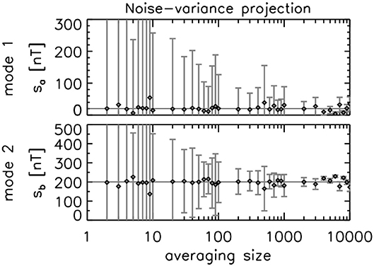
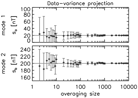
Signal amplitudes for the two modes are obtained using the noise variance projection (Equation 52) and the data variance projection (Equation 52), and are graphically displayed as a function of the averaging size (or the number of realizations or samples) in Figures 4, 5 together with the one-sigma errors. The both estimators can find the true signal amplitudes (20 nT for the mode 1 and 200 nT for the mode 2) within the error bar, and the analysis using a larger statistical sampling size is beneficial in reducing the error. Yet, the accuracy is by far improved in the data-variance projection. The error bar is about 10 nT for an averaging size of 10–100 and becomes only a few nT or better (cf. the noise amplitude is 1 nT) for an even larger averaging size in the data-variance projection. The estimated amplitudes sufficiently converge to the true values for averaging sizes above 10, too. In contrast, the noise-variance projection still exhibits random deviations of the signal amplitudes from the true values for a larger averaging size (for example, size of 1,000).

FIGURE 4

Figure 4. Amplitudes for the mode 1 (constant field from the current sheet) and the mode 2 (dipolar field at the planetary surface) estimated by the noise-variance projection as a function of the averaging size.

FIGURE 5

Figure 5. Amplitudes for the mode 1 and the mode 2 (the same format as Figure 4) estimated by the data-variance projection.

4. Outlook

Capon's projection is a useful tool when the noise property is unknown, and has a higher flexibility for various applications and extensions compared to the beamforming or the MSR methods. The extension of the minimum variance projection onto a multitude of shape vectors in the data opens the door to a decomposition method for the multi-point data. An application is presented for a decomposition of the multi-point data into a constant magnetic field and a dipolar field in view of the Mercury magnetosphere. It is comforting that even two-point measurements are capable of identifying the signal amplitudes when a sufficient amount of data is obtained for the proper averaging operation.

Another application is a decomposition into a set of orthogonal function basis. Capon estimator and its extension to the mode decomposition can be applied to various wave fields in the solar wind, the foreshock, the magnetosheath, and the magnetotail regions as well as various static fields as far as the spatial structure can be properly modeled (such as the dayside magnetosphere as presented in this paper). For example, the source locator uses the lowest-order spherical Bessel function j₀(x) = sin(x)/x and the lowest-order Neumann function n₀(x) = −j₋₁(x) = −cos(x)/x. The expansion into a series of spherical Bessel functions or cylindrical functions (presumably with a cutoff) is a possible application to the multi-point measurements, e.g., identification or reconstruction of the spherical propagation or the vortical shape or motion.

Capon's minimum variance projection is not limited to the search for wave propagations or mode decomposition into different sources of the magnetic fields, but the method can be applied to solitary, spatially-localized structures. A useful example may be the KdV (Korteweg-de Vries) soliton (or ion-acoustic solitons in the case of plasmas) characterized by the following shape vector, $h_i(A,D,c,x_0)=A\text{sec}{\text{h}}^2\left[D(x_i-ct+x_0)\right]$ where c is the phase speed of the propagation, A the amplitude, and D the width of the soliton structure around the peak. The amplitude and the width are determined by the phase speed. For ion-acoustic solitons, the amplitude is given as A = 3c and the width $D=\sqrt{c/2}$ [21].

Author Contributions

The author confirms being the sole contributor of this work and has approved it for publication.

Conflict of Interest Statement

The author declares that the research was conducted in the absence of any commercial or financial relationships that could be construed as a potential conflict of interest.

Acknowledgments

Discussions with Tohru Hada, Uwe Motschmann, and Daniel Heyner are greatly acknowledged to improve the quality of the manuscript.

References

1. Capon J. High resolution frequency-wavenumber spectrum analysis. Proc IEEE (1969) 57:1408–18. doi: 10.1109/PROC.1969.7278

CrossRef Full Text | Google Scholar

2. Angelopoulos V. The THEMIS mission. Space Sci Rev. (2008) 141:5–34. doi: 10.1007/s11214-008-9336-1

CrossRef Full Text | Google Scholar

3. Friis-Christensen E, Lühr H, Hulot G. Swarm: a constellation to study the Earth's magnetic field. Earth Planets Space (2006) 58:351–8. doi: 10.1186/BF03351933

CrossRef Full Text | Google Scholar

4. Friis-Christensen E, Lühr H, Knudsen D, Haagmans R. Swarm–an earth observation mission Investigating geospace. Adv Space Res. (2008) 41:210–6. doi: 10.1016/j.asr.2006.10.008

CrossRef Full Text | Google Scholar

5. Escoubet CP, Fehringer M, Goldstein M. Introduction to the cluster mission, Ann Geophys. (2001) 19:1197–200. doi: 10.5194/angeo-19-1197-2001

CrossRef Full Text | Google Scholar

6. Burch JL, Moore TE, Torbert RB, Giles BL. Magnetospheric multiscale overview and science objectives. Space Sci Rev. (2016) 199:5–21. doi: 10.1007/s11214-015-0164-9

CrossRef Full Text | Google Scholar

7. Haykin S. Adaptive Filter Theory, 2nd. ed., Prentice Hall Information and System Science Series. Upper Saddle River, NJ: Prentice-Hall Inc. (1991).

Google Scholar

8. Khmou Y, Safi S, Frikel M. Comparative study between several direction of arrival estimation methods. J Telecomm Inform Tech. (2014) 2014:41–8.

Google Scholar

9. Narita Y, Glassmeier KH, Motschmann U. Wave vector analysis methods using multi-point measurements. Nonlin Processes Geophys. (2010) 17:383–94. doi: 10.5194/npg-17-383-2010

CrossRef Full Text | Google Scholar

10. Motschmann U, Woodward TI, Glassmeier KH, Dunlop MW. Array signal processing techniques. In: Glassmeier KH, Motschmann U, Schmidt R. editors. Proceedings of the Cluster Workshop on Data Analysis Tools, Braunschweig (1995). ESA SP-371, p. 79–86. p. 28–3.

Google Scholar

11. Narita Y, Glassmeier KH, Motschmann U. High-resolution wave number spectrum using multi-point measurements in space–the multi-point signal resonator (MSR) technique. Ann Geophys. (2011) 29:351–60. doi: 10.5194/angeo-29-351-2011

CrossRef Full Text | Google Scholar

12. Motschmann U, Woodward TI, Glassmeier KH, Southwood DJ, Pinçon J. Wavelength and direction filtering by magnetic measurements at satellite arrays: generalized minimum variance analysis. J Geophys Res. (1996) 101:4961–6. doi: 10.1029/95JA03471

CrossRef Full Text | Google Scholar

13. Glassmeier KH, Motschmann U, Dunlop M, Balogh A, Acuña MH, Carr C, et al. Cluster as a wave telescope–first results from the fluxgate magnetometer. Ann Geophys. (2001) 19:1439–47. doi: 10.5194/angeo-19-1439-2001

CrossRef Full Text | Google Scholar

14. Pinçon JL, Lefeuvre F. Local characterization of homogeneous turbulence in a space plasma from simultaneous measurements of field components at several points in space. J Geophys Res. (1991) 96:1789–802. doi: 10.1029/90JA02183

CrossRef Full Text | Google Scholar

15. Constantinescu OD, Glassmeier KH, Motschmann U, Treumann RA, Fornaçon KH, Fränz M. Plasma wave source location using CLUSTER as a spherical wave telescope. J Geophys Res Space Phys. (2006) 111:A09221. doi: 10.1029/2005JA011550

CrossRef Full Text | Google Scholar

16. Constantinescu OD, Glassmeier KH, Décréau PME, Fränz M, Fornaçon KH. Low frequency wave sources in the outer magnetosphere, magnetosheath, and near Earth solar wind. Ann Geophys. (2007) 25:2217–28. doi: 10.5194/angeo-25-2217-2007

CrossRef Full Text | Google Scholar

17. Plaschke F, Glassmeier KH, Constantinescu OD, Mann IR, Milling DK, Motschmann U, et al. Statistical analysis of ground based magnetic field measurements with the field line resonance detector. Ann Geophys. (2008) 26:3477–89. doi: 10.5194/angeo-26-3477-2008

CrossRef Full Text | Google Scholar

18. Capon J, Greenfield RJ, Kolker RJ. Multidimensional maximul-likelihood processing of a large aperture seismic array. Proc IEEE (1967) 55:192–211. doi: 10.1109/PROC.1967.5439

CrossRef Full Text | Google Scholar

19. Dodelson S. Modern Cosmology. London: Academic Press (2003).

Google Scholar

20. Benkhoff J, van Casteren J, Hayakawa H, Fujimoto M, Laakso H, Novara M, et al. BepiColombo–comprehensive exploration of mercury: mission overview and Science goals. Planet Space Sci. (2010) 58:2–20. doi: 10.1016/j.pss.2009.09.020

CrossRef Full Text | Google Scholar

21. Ichikawa YH, Watanabe S. Solitons, envelope solitons in collisionless plasmas. J Phys Colloques (1977) 38:15–26. doi: 10.1051/jphyscol:1977603

CrossRef Full Text | Google Scholar

Appendix: Derivative Calculation

Calculation for Equation 40 is as follows. The first-order derivative of the Gaussian error likelihood function (Equation 39) with respect to the variance C_S is obtained:

$\begin{array}{l}\frac{\partial L}{\partial C_{\text{R}}}=\frac{n/2}{{(C_{\text{R}}+C_{\text{N}})}^{n/2-1}}\exp \left[-\frac{1}{2}\frac{\langle {\sum }_{i=1}^n{\left(d_i-h_{i}s\right)}^2\rangle }{C_{\text{R}}+C_{\text{N}}}\right]+\\ \frac{1}{2}\frac{1}{{(C_{\text{R}}+C_{\text{N}})}^{n/2}}\frac{\langle {\sum }_{i=1}^n{\left(d_i-h_{i}s\right)}^2\rangle }{{(C_{\text{R}}+C_{\text{N}})}^2}\times \\ \exp \left[-\frac{1}{2}\frac{\langle {\sum }_{i=1}^n{\left(d_i-h_{i}s\right)}^2\rangle }{C_{\text{R}}+C_{\text{N}}}\right]& (\text{A}1)\end{array}$

$\begin{array}{lll}=& {L}\left[-\frac{n}{2(C_{\text{R}}+C_{\text{N}})}+\frac{\langle {\displaystyle {\sum }_{i=1}^n}{(d_i-h_{i}s)}^2\rangle }{2{(C_{\text{R}}+C_{\text{N}})}^2}\right].& (\text{A}2)\end{array}$

The second-order derivative of the logarithmic of the likelihood function is:

$\begin{array}{ll}\frac{{\partial }^2(ln{L})}{\partial C_{\text{R}}^2}=\frac{\partial }{\partial C_{\text{R}}}\left[\frac{1}{{L}}\frac{\partial {L}}{\partial C_{\text{R}}}\right]& (\text{A}3)\end{array}$

$\begin{array}{lll}=& \frac{\partial }{\partial C_{\text{R}}}\left[\frac{-n/2}{C_{\text{R}}+C_{\text{N}}}+\frac{1}{2}\frac{\langle {\displaystyle {\sum }_{i=1}^n}{(d_i-h_{i}s)}^2\rangle }{{(C_{\text{R}}+C_{\text{N}})}^2}\right]& (\text{A}4)\end{array}$

$\begin{array}{lll}=& \frac{n}{2}\frac{1}{{(C_{\text{R}}+C_{\text{N}})}^2}-\frac{n}{{(C_{\text{R}}+C_{\text{N}})}^2}& (\text{A}5)\end{array}$

$\begin{array}{lll}=& \frac{n}{2}\frac{1}{{(C_{\text{R}}+C_{\text{N}})}^2}.& (\text{A}6)\end{array}$

Here the first-order derivative evaluated at the peak of the likelihood function, $\partial {L}/\partial C_{\text{R}}=0$, i.e.,

$\begin{array}{ll}\langle {\displaystyle \sum _{i=1}^n}{(d_i-h_{i}s)}^2\rangle =n(C_{\text{R}}+C_{\text{N}})& (\text{A}7)\end{array}$

is used in deriving Equation (A5). The one-sigma error (Equation 40) is evaluated using Equation (A6).