Polarization Rotation and Mode Splitting in Photonic Crystal Line-Defect Waveguides

In a line-defect waveguide of a planer photonic crystal (PhC), we found a new rotational state of polarized light, which exhibits “polarization rotation” on the PhC plane, when a phase mismatch m was added to the air-hole alignment of the waveguide, where mode splitting was simultaneously observed in the dispersion curve. To account for the polarization rotation together with the mode splitting, we propose a two-state model that is constructed from Schrödinger equation obtained from the equation for electromagnetic waves. The proposed two-state model gives an explanation on the relation between the polarization-rotational angle θ and the mismatch m and on its rotational direction (i.e., clockwise or anticlockwise direction) that depends on the mode. Using the two-state model, we also discuss the angular momenta of the polarized light in the PhC waveguide, which are directly related to the Stokes parameters that characterize the polarization rotations.

1. Introduction

In a line-defect waveguide of a planer photonic crystal (PhC), the polarization of light can rotate on the two dimensional PhC plane by addition of a phase mismatch to the air-hole alignment of the waveguide, which occurs without non-linear optical interactions (e.g., optical Kerr effects and photorefractive effects). Originally, the presence of light rotation, given as an optical vortex that carries angular momentum, in photonic bandgap media [1–4] via such non-linear interactions has been found in theoretical and experimental investigations [5–9, 10]; This mechanism is attributed to the localized vortex state induced by those non-linear effects in the bandgap media, which is thus sometimes called a gap vortex. This is an analogous concept to a gap soliton in the bandgap media [11, 12].

However, without such non-linear effects, we can show the presence of a rotational state of polarized light just by adding the mismatch m (0 < m < a) to the air-hole alignment of a sidewall of the waveguide [13], as illustrated in Figure 1, where a is the air-hole period of the PhC waveguide. Mock et al. also studied the same waveguide [14], but did not report such rotation. They just reported that the light path in the waveguide was “zigzag.” An interesting feature of the rotation that we found is that if light propagates from a non-mismatched region to the mismatched region with a gradual mismatch change between them, the light polarization gradually rotates. Here we can define its rotational angle θ for a given m, and as will be shown later, θ is proportional to m (for small m compared with a) via numerical simulations.

FIGURE 1

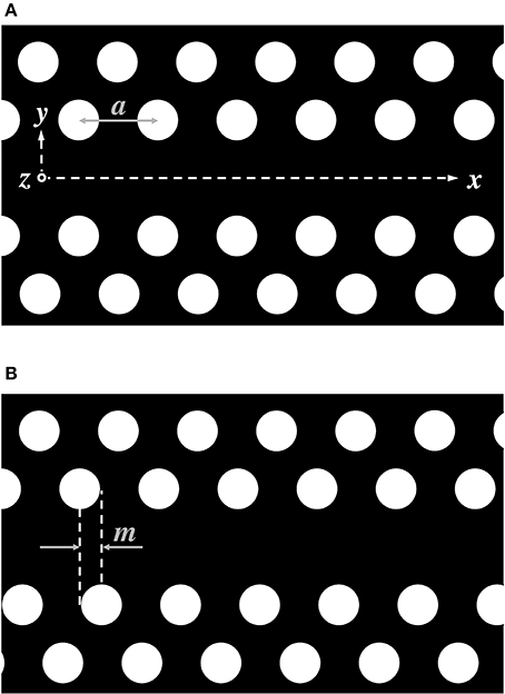
Figure 1. PhC line-defect waveguides, where light propagates through the central part in the x-direction. The white circles are air-holes made on a black material (e.g., silicon), where the air-hole spacing (or lattice constant) is a, and the air-hole diameter is assumed to be smaller than a. (A) Air-hole alignments are symmetric with respect to the central line (or the x-axis). (B) The lower part of the air-hole alignment is shifted with the addition of a mismatch m, which causes the polarization rotation of light.

Moreover, with the addition of m, mode splitting (or level splitting) is observed in the dispersion curve [13, 14], which is created from an originally degenerated mode that contains different polarizations. The main cause of this mode splitting is symmetry breaking; When m = 0, structural symmetry in the x and y directions is maintained (despite the presence of a line-defect waveguide at y = z = 0), which causes highly degenerated states in the dispersion curve. But, structural symmetry breaking caused by m ≠ 0 can resolve the degenerated states, creating two split modes, as will be shown in detail in section 2.

We infer from our numerical simulations that the polarization rotation is intimately connected with the mode splitting, because they occur simultaneously, triggered by the addition of m. (Because of the above reasons, the mechanism of the rotational light obtained in our research is completely different from that of a gap vortex with non-linear interactions; the rotation that we found is spatial rotation, not temporal rotation seen for the localized vortex.)

In this paper, we will gain a qualitative understanding of the simultaneous polarization rotation and mode splitting from our two-state model constructed via Schrödinger equation derived from the equation for electromagnetic (EM) waves in the waveguide. In this analysis, we can show that there is a relation between the polarization-rotational angle θ and the mismatch m (via a relation between the mode-splitting spacing ω and the mismatch m), which is an analogous relation to that between an electron-energy-level splitting ℏω and an applied magnetic field B, or ℏ ω∝ B.

In the next section, we will give some numerical simulation results, and then introduce a theory that connects the mode splitting with the polarization rotation within linear optics.

2. Numerical Results for Mode Splitting and Polarization Rotation

Finite-difference time-domain computations [13, 14] show that when m = 0, the band structure (or the dispersion curve) of a PhC line-defect waveguide has mode-crossing points, as depicted in Figure 2. Each of the mode-crossing points consists of two degenerated modes with different polarizations, which are yielded by band-folding (realized in the reduced zone for the wavenumber k at − π/a ≤ k ≤ π/a). With the addition of non-zero m, the two-fold degeneracy is resolved (see Figure 2), thereby creating two split modes, where the gap size f between the split modes increases with increasing m. (Schematic diagrams of Figure 3 well describe this behavior, and show that the mode splitting can be regarded as level splitting). The electric fields with different polarizations (with even or odd modes) come to what we call TE${}_1^{-}$ or TE${}_1^{+}$, respectively, as displayed in Figure 4 for k = 0.2925 × 2π/a at m/a = 0, 1/8, 1/4, 3/8, 1/2. (Much clearer polarization rotation can be seen in H_z, and this will also be shown below.)

FIGURE 2

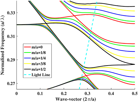
Figure 2. Band structure of the PhC line-defect waveguide. Here, the air-hole period a is 450 nm, the air-hole radius is 0.29a, and the waveguide width is $1.2\sqrt{3}a$. Mode-crossing points exist for m/a = 0. As m increases (e.g., m/a = 1/8, 1/4, 3/8, 1/2), each mode-crossing point splits into two modes (the upper and lower modes) and the split-mode spacing (or gap size) becomes large. The light line for the waveguide with upper and lower air-claddings is indicated by the slanted dashed line.

FIGURE 3

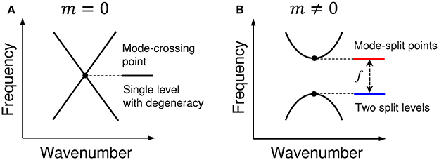
Figure 3. Schematic diagrams for (A) a mode-crossing point with m = 0, which can be regarded as a single level with degeneracy, and (B) mode-split points with m≠0, which can be looked upon as two split levels.

FIGURE 4

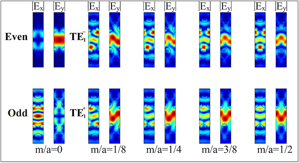
Figure 4. Electric fields with different polarizations that come to the TE${}_1^{-}$- and TE${}_1^{+}$-polarizations with even and odd modes, respectively, for m/a = 0, 1/8, 1/4, 3/8, 1/2 at k = 0.2925 × 2π/a. Here, the absolute value of E_x and E_y is plotted.

Figure 5 with the blue (TE${}_1^{+}$) and red (TE${}_1^{-}$) curves depicts a calculated m-dependence of the split modes, TE${}_1^{+}$ and TE${}_1^{-}$, that correspond to those in Figure 3B, which are produced from the lowest degenerated TE₁ mode at 190.13 THz with k = 0.2925 × 2π/a. Here, we chiefly focus on the lowest mode (TE₁) because its crossing point at 190.13 THz with k = 0.2925 × 2π/a is placed inside the light cone, that is, the light at that point is a really-propagating mode, not a radiation mode. Also, we observed that a maximum gap size f_max = 8.68 THz was obtained at m/a = 0.5 and that the splitting behavior was symmetric for (a) 0 < m/a ≤ 0.5 and (b) 0.5 < m/a < 1. Thus we plotted the figure for Case (a) only, which is sufficient to look at the essence of the behavior. The inset of Figure 5 shows the m-dependence of the normalized gap size, f/f_max. Here, we phenomenologically found that it had good linearity, i.e., f/f_max = gm/a (g = 2.5615) at m/a ≲ 0.3 (but f/f_max leveled off near m/a = 0.5). The g = 2.5615 was obtained via the least square fitting with a straight line for the data points at m/a less than or equal to 0.2875. Note that we also observed that the center (say $\bar{\Omega }=({\Omega }_0+{\Omega }_1)/2$) of the TE${}_1^{+}$ and TE${}_1^{-}$ modes (say Ω₀ and Ω₁) showed little m-dependence (almost no m-dependence), as indicated by the black dashed curve in Figure 5 (although Ω₁−Ω₀ = ω = 2πf showed a large m-dependence, as seen in Figure 5).

FIGURE 5

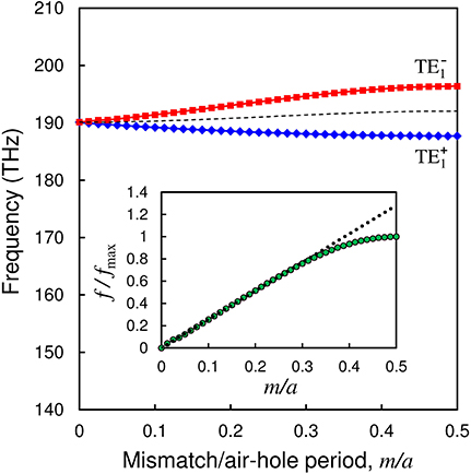
Figure 5. Calculated m-dependence of the two split modes, TE${}_1^{+}$ (blue curve) and TE${}_1^{-}$ (red curve), produced from a mode-crossing point at 190.13 THz with k = 0.2925 × 2π/a of a degenerated TE₁ mode. The centre of the TE${}_1^{+}$ and TE${}_1^{-}$ modes has little m-dependence, as indicated by the black dashed curve. The gap size f between the TE${}_1^{+}$ and TE${}_1^{-}$ modes increases with m, and the maximum gap size f_max(= 8.68THz) is obtained at m/a = 0.5. The inset shows the m-dependence of f/f_max by the green dots, where the green dots at m/a≲ 0.3 fit well with the black dashed line with f/f_max = gm/a (g = 2.5615).

We then give clearer field and intensity profiles of the TE${}_1^{-}$ and TE${}_1^{+}$ modes for H_z: Figure 6A shows the field profile or the real part of H_z in a unit cell at k = π/a of the Brillouin-zone (BZ) end, and Figure 6B shows the intensity profile $|H_z{|}^2$ at a mode-crossing point, k = 0.2925 × 2π/a. We then observe clearer tilted field and intensity profiles with a tilted angle (or a rotational angle) θ that increases with increasing m. In this case, we found that the rotation of the intensity profiles of TE${}_1^{+}$ (TE${}_1^{-}$) in Figure 6B was in the anticlockwise (clockwise) direction; A similar tendency remained in the field rotations of Figure 6A at the BZ end (since we observed in numerical simulations that the mode-splitting spacing became large even at the BZ end as m increased).

FIGURE 6

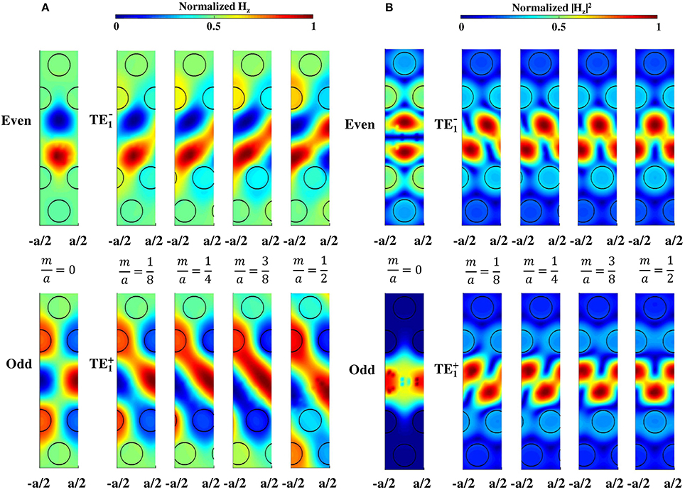
Figure 6. Mode profiles of TE${}_1^{+}$ and TE${}_1^{-}$ at m/a = 0, 1/8, 1/4, 3/8, 1/2 (for odd and even modes). (A) Field profile of the real part of H_z at k = π/a of the BZ end. (B) Intensity $|H_z{|}^2$ at k = 0.2925 × 2π/a of a crossing point.

The above results were obtained only from the numerical simulations (i.e., with no theoretical explanations via analytical methods). In the next section, we will explain the observed simultaneous polarization rotation and mode splitting by use of an analytical method with a two-state model derived from the equation for EM waves.

3. Analytical Interpretation and Discussion

To derive the two-state model to account for the above phenomena, we start with the following wave equation (obtained from Maxwell's equations) for light propagating in the x direction with polarization E_i:

$\begin{array}{cc}\begin{array}{r}({\nabla }^2-\frac{n^2}{c^2}\frac{{\partial }^2}{\partial t^2})E_i=0,\end{array}& (1)\end{array}$

where ∇² = ∂²/∂x²+∂²/∂y²+∂²/∂z², n is the refractive index that includes the PhC spatial modulation, and c is the velocity of light.

In the following, we make an approximation that the input-pulse spatial-width W(> λ) is larger than the air-hole period a in the waveguide, where the input wavelength λ also needs to suffices λ > a. This approximation makes it possible to deal with the phenomenon (light rotation) analytically, but cannot well describe it near the PhC band edge because the backward reflection of propagating light is strong due to Bragg reflection with the air-hole arrays. Within the above approximation, an average nature of the rotation of light in a size of order ~ λ can be obtained.

While keeping the above approximation, we insert $E_i=u_i{e}^{i(\beta x-wt)}$ into Equation (1) and obtain the next Schrödinger equation [15] (see Appendix):

$\begin{array}{cc}\begin{array}{rcl}i\hslash \frac{\partial u_i}{\partial t}& =& -\frac{{\hslash }^2}{2n_{\text{eff}}}{\nabla }_2^2{u}_i+V{u}_i\end{array}& (2)\end{array}$

$\begin{array}{cc}\begin{array}{rc}\equiv & H(t)u_i,\end{array}& (3)\end{array}$

where we used the notations: ℏ ≡ λ/2π, t≡ x, V≡ n_eff−n, β = n_effk = 2πn_eff/λ, ${\nabla }_2^2={\partial }^2/\partial y^2+{\partial }^2/\partial z^2$, and n_eff is the effective refractive index in the waveguide. Here we also used the slowly-varying-envelope approximation, $|{\partial }^2{u}_i/\partial x^2|\ll |2\beta \partial u_i/\partial x|$. In addition, we omitted a small difference in β for waves with different polarizations (and with the same node numbers). In this situation, we can perfectly utilize ideas and descriptions in quantum mechanics to study the phenomena. Hereafter, we will deal with all quantities in units of ℏ = c = 1, as often used in quantum mechanics.

Now we concentrate on the lowest eigenvalue of the right-hand side of Equation (2) when m = 0, as described in section 2. In this case, we denote $\bar{\Omega }$ as the lowest eigenvalue, or the lowest frequency at the crossing point (with m = 0). When m is added (i.e., m≠0), since the mode with $\bar{\Omega }$ with degeneracy splits into two modes, we set their eigenvalues to be Ω₀ and Ω₁, where ${\Omega }_0=\bar{\Omega }-\omega /2$ and ${\Omega }_1=\bar{\Omega }+\omega /2$ with a gap size of ω(= 2πf) between the two split modes, where ω has a large m-dependence but $\bar{\Omega }$ has little m-dependence, as already shown in Figure 5.

For those two split modes, the Hamiltonian H(t) in Equation (3) can be written in the matrix representation as

$\begin{array}{cc}\begin{array}{l}H(t)=\left(\begin{array}{cc}{\Omega }_1& 0\\ 0& {\Omega }_0\end{array}\right)\\ =\frac{{\Omega }_1+{\Omega }_0}{2}\widehat{1}+\frac{{\Omega }_1-{\Omega }_0}{2}\widehat{\sigma }3\\ \begin{array}{cc}=& \stackrel{}{\overline{\Omega }}\widehat{1}+\omega \frac{\widehat{\sigma }}{2},\end{array}\end{array}& (4)\end{array}$

which is known as a two-state model [16]. In Equation (4), $\widehat{1}$ is a unit matrix and $\widehat{\sigma }$ is the z-component of the Pauli matrices (${\widehat{\sigma }}_1$, ${\widehat{\sigma }}_2$, ${\widehat{\sigma }}_3$):

$\begin{array}{cc}\begin{array}{c}\widehat{\sigma }1=\left(\begin{array}{cc}0& 1\\ 1& 0\end{array}\right),\widehat{\sigma }2=\left(\begin{array}{cc}0& -i\\ i& 0\end{array}\right)\end{array},\widehat{\sigma }3=\left(\begin{array}{cc}1& 0\\ 0& -1\end{array}\right)& (5)\end{array}$

that suffice

$\begin{array}{cc}\begin{array}{r}\left[{\widehat{\sigma }}_i,{\widehat{\sigma }}_j\right]=2i{ϵ}_{ijk}{\widehat{\sigma }}_k,\end{array}& (6)\end{array}$

$\begin{array}{cc}\begin{array}{r}\left\{{\widehat{\sigma }}_i,{\widehat{\sigma }}_j\right\}=2{\delta }_{ij}\widehat{1}\end{array}& (7)\end{array}$

and thus

$\begin{array}{cc}\begin{array}{r}{\widehat{\sigma }}_i\widehat{{\sigma }_j}={\delta }_{ij}\widehat{1}+i{ϵ}_{ijk}{\widehat{\sigma }}_k,\end{array}& (8)\end{array}$

where [X, Y] = XY − YX, {X, Y} = XY + YX, and i, j, k run from 1 to 3. ϵ_ijk is the Levi-Civita symbol, and δ_ij is the Kronecker delta. In what follows, we also use the vector notation of Equation (5), i.e., $\widehat{\sigma }=({\widehat{\sigma }}_1,{\widehat{\sigma }}_2,{\widehat{\sigma }}_3)$.

For the Hamiltonian (4), the Schrödinger equation is of the form:

$\begin{array}{cc}\begin{array}{rcl}i\frac{d}{dt}|\varphi (t)\rangle & =& {H}(t)|\varphi (t)\rangle ,\end{array}& (9)\end{array}$

$\begin{array}{cc}\begin{array}{rc}=& (\bar{\Omega }\widehat{1}+\omega \frac{{\widehat{\sigma }}_3}{2})|\varphi (t)\rangle ,\end{array}& (10)\end{array}$

where |ϕ(t)〉 is a two-component wave function, or a spinor [17, 18]. (Its detail is described below.) In Equation (10), using the following transformation

$\begin{array}{cc}\begin{array}{r}|\varphi (t)\rangle =e^{-i\bar{\Omega }\widehat{1}t}|\psi (t)\rangle =e^{-i\bar{\Omega }t}|\psi (t)\rangle ,\end{array}& (11)\end{array}$

we can simplify the Equation (10) as

$\begin{array}{cc}\begin{array}{r}i\frac{d}{dt}|\psi (t)\rangle ={H}(t)|\psi (t)\rangle ,\end{array}& (12)\end{array}$

where

$\begin{array}{cc}\begin{array}{r}{H}(t)=\omega \frac{{\widehat{\sigma }}_3}{2}.\end{array}& (13)\end{array}$

In Equation (11), deriving the $e^{-i\bar{\Omega }t}$-term from |ϕ(t)〉 is accepted, because we observed a sizable field/intensity tilt induced by a change in m or ω (because ω has a large m-dependence, but not $\bar{\Omega }$ because $\bar{\Omega }$ has little m-dependence). Thus clearly, we can say that the tilt does not depend on $\bar{\Omega }$. Furthermore, when we calculate the expectation value for an operator $\widehat{{B}}$, we can rigorously say that no $\bar{\Omega }$ term contributes to the expectation value: In fact, we obtain via the transformation (11).

$\begin{array}{cc}\langle \widehat{\mathcal{O}}\rangle t=\langle \varphi (t)|\widehat{\mathcal{O}}|\varphi (t)\rangle =\langle \psi (t)|\widehat{\mathcal{O}}|\psi (t)\rangle .& (14)\end{array}$

Further, at the initial state (or at t = 0), the next relation holds:

$\begin{array}{cc}\begin{array}{r}|\varphi (0)⟩=|\psi (0)⟩\equiv |\psi ⟩,\end{array}& (15)\end{array}$

where |ψ〉 is the (time-independent) eigenvector of Equation (13), or a spinor:

$\begin{array}{cc}\begin{array}{c}|\psi \rangle =\left(\begin{array}{c}{u}_1\\ u_2\end{array}\right).\end{array}& (16)\end{array}$

Here, u₁ and u₂ are polarized electric fields or wave functions that will come into the TE${}_1^{-}$ mode and TE${}_1^{+}$ mode, respectively. Equation (16) is almost the same as the Jones vector constructed with polarized electric fields, which is expressed as a spinor with an appropriate basis [19, 20]. There is a slight difference in definition between Equation (16) and the Jones vector defined with plane EM waves, because our EM waves are the waves propagating along the PhC waveguide with different polarization directions; nonetheless, almost the same definition can be used (except for the polarization directions).

The above spinor of a two-state model with Equation (13) can be regarded as that of an electron with spin $\frac{1}{2}$. In this case, as is well-known, the size of ω in Equation (13) is proportional to the strength B of an applied magnetic field, i.e., ω ∝ B (for weak B) [16]. In this situation, we can look upon m as B phenomenologically by help of the “equivalence” between ω ∝ m and ω ∝ B (for small m and B).

Next, to see the time evolution of the system with H(t), we use the following equation for a unitary operator U(t) [16, 21].

$\begin{array}{cc}\begin{array}{r}i\frac{d}{dt}U(t)={H}(t)U(t).\end{array}& (17)\end{array}$

Equation (17) can be derived from the derivative of the identity $U{(t)}^{†}U(t)=U(t)U{(t)}^{†}=\widehat{1}$, that is,

$\begin{array}{cc}\begin{array}{r}i\frac{dU(t)}{dt}U{(t)}^{†}=-iU(t)\frac{dU{(t)}^{†}}{dt},\end{array}& (18)\end{array}$

which indicates that the left-hand side of Equation (18) is hermitian. If we set this hermitian part as H(t), Equation (17) can be obtained from Equation (18).

By inserting Equation (13) into Equation (17) and integrating Equation (17) with the initial condition $U(0)=\widehat{1}$, we obtain

$\begin{array}{cc}U(t)=\widehat{1}-i{\displaystyle {\int }_0^{t}d}{t}_1\mathscr{H}(t_1)+{(-i)}^2{\displaystyle {\int }_0^{t}d}{t}_1{\displaystyle {\int }_0^{t_1}d}{t}_2\mathscr{H}(t_1)\mathscr{H}(t_2)+\dots & (19)\end{array}$

$\begin{array}{cc}\begin{array}{rc}=& {\displaystyle \sum _{n=0}^{\infty }}{(-i)}^n{(\omega \frac{{\widehat{\sigma }}_3}{2})}^n\frac{t^n}{n!}\end{array}& (20)\end{array}$

$\begin{array}{cc}\begin{array}{rc}=& e^{-i\omega \frac{{\widehat{\sigma }}_3}{2}t}\end{array}& (21)\end{array}$

$\begin{array}{cc}\begin{array}{rc}=& \widehat{1}cos\frac{\omega t}{2}-i{\widehat{\sigma }}_{3}sin\frac{\omega t}{2},\end{array}& (22)\end{array}$

where the time-integration parts have been simply calculated as

$\begin{array}{cc}{\displaystyle {\int }_0^{t}d}{t}_1{\displaystyle {\int }_0^{t_1}d}{t}_2\dots {\displaystyle {\int }_0^{t_{n-1}}d}{t}_n=\frac{t^n}{n!}& (23)\end{array}$

because ${H}(t)=\omega {\widehat{\sigma }}_3/2$ has no time-dependence.

In this case, the time-evolution |ψ(t)⟩ of the spinor |ψ⟩ in Equation (16) is of the form:

$\begin{array}{cc}\begin{array}{rcl}|\psi (t)\rangle & =& U(t)|\psi \rangle \end{array}& (24)\end{array}$

$\begin{array}{cc}\begin{array}{rc}=& e^{-i\omega \frac{{\widehat{\sigma }}_3}{2}t}|\psi \rangle \end{array}& (25)\end{array}$

$\begin{array}{cc}\begin{array}{rc}=& (\widehat{1}cos\frac{\omega t}{2}-i{\widehat{\sigma }}_{3}sin\frac{\omega t}{2})|\psi \rangle .\end{array}& (26)\end{array}$

where if we interpret that ωt is an angle θ for the polarization rotation, then Equation (26) gives a double-valuedness to u₂ (or u₁) in the θ-rotation. Here, t should be interpreted as the length of the interconnection part between the non-mismatched entrance and the mismatched exit (when we use the units of ℏ = c = 1); The “t” is a constant when the interconnection length has a fixed value. Even in this situation, θ can vary as m changes because the insertion of f = g f_max m/a into ω = 2πf in Equation (26) gives θ = ωt = 2πgf _maxtm/a = θ₀m/a, where θ₀ = 2πgf _maxt is a constant. Inserting ωt = θ into Equation (26), we obtain

$\begin{array}{cc}\begin{array}{r}|\psi (\theta )\rangle =(\widehat{1}cos\frac{\theta }{2}-i{\widehat{\sigma }}_{3}sin\frac{\theta }{2})|\psi \rangle ,\end{array}& (27)\end{array}$

which provides the relation |ψ(2π)⍹ = −|ψ(0)⟩. Furthermore, Equation (27) can explain the aforementioned anticlockwise (clockwise) rotation of the TE${}_1^{+}$ (TE${}_1^{-}$) mode, because the explicit expression of Equation (27) with

$\begin{array}{cc}\begin{array}{c}|\psi (\theta )\rangle =\left(\begin{array}{c}{u}_1(\theta )\\ u_2(\theta )\end{array}\right),|\psi \rangle =\left(\begin{array}{c}{u}_1\\ u_2\end{array}\right)\end{array}& (28)\end{array}$

is of the form:

$\begin{array}{cc}\left(\begin{array}{c}{u}_1(\theta )\\ u_2(\theta )\end{array}\right)=\left(\begin{array}{c}{e}^{-i\theta /2}{u}_1\\ e^{i\theta /2}{u}_2\end{array}\right).& (29)\end{array}$

Thus, if u₂(θ) rotates anticlockwise, then u₁(θ) rotates clockwise (and vice versa). Note that in terms of |ϕ(t)⟩ (not |ψ(t)⟩), we obtain in place of Equation (29):

$\begin{array}{cc}\left(\begin{array}{c}{u}_1(\theta )\\ u_2(\theta )\end{array}\right)=\left(\begin{array}{c}{e}^{-i{\Theta }_0}{e}^{-i\theta /2}{u}_1\\ e^{-i{\Theta }_0}{e}^{i\theta /2}{u}_2\end{array}\right),& (30)\end{array}$

where ${\Theta }_0=\bar{\Omega }t$ is a constant when the “length” t is a constant, as described above. If m = 0, then θ = 0, but Θ₀ remains as a constant (because $\bar{\Omega }$ in Θ₀ has (almost) no m-dependence); in this case (or m = 0), Equation (30) becomes

$\begin{array}{cc}\left(\begin{array}{c}{u}_1(0)\\ u_2(0)\end{array}\right)=\left(\begin{array}{c}\begin{array}{c}{e}^{-i{\Theta }_0}{u}_1\\ e^{-i{\Theta }_0}{u}_2\end{array}\end{array}\right).& (31)\end{array}$

Equation (31) corresponds to the zero-m fields, as given at the leftmost ones in Figure 6A. We can see that adjusting the parameter “t” in Θ₀ of Equation (31) enables setting various initial polarized states at m = 0. We should examine the field tilt for m ≠ 0 as a difference from those initial field profiles, (u₁(0)u₂(0)), and thus what we should look upon as a field tilt is given by

$\begin{array}{cc}\left(\begin{array}{c}{u}_1(\theta )\\ u_2(\theta )\end{array}\right)\begin{array}{c}=\left(\begin{array}{c}{e}^{-i\theta /2}{u}_1(0)\\ e^{i\theta /2}{u}_2(0)\end{array}\right),\end{array}& (32)\end{array}$

and hence we obtain the same result as that in Equation (29).

As for the evolution of the angular momentum operator $\widehat{\sigma }$, we can calculate it as

$\begin{array}{cc}\begin{array}{r}\widehat{\sigma }(t)=U^{†}(t)\widehat{\sigma }U(t).\end{array}& (33)\end{array}$

Using Equations (21),(33), we obtain

$\begin{array}{cc}\left(\begin{array}{c}{\widehat{\sigma }}_1(t)\\ {\widehat{\sigma }}_2(t)\\ {\widehat{\sigma }}_3(t)\end{array}\right)=\left(\begin{array}{ccc}\cos \omega t& -\sin \omega t& 0\\ \sin \omega t& \cos \omega t& 0\\ 0& 0& 1\end{array}\right)\left(\begin{array}{c}{\widehat{\sigma }}_1\\ {\widehat{\sigma }}_2\\ {\widehat{\sigma }}_3\end{array}\right),& (34)\end{array}$

where Equations (8),(22) have been used in the calculations. For convenience, we rewrite Equation (34) as

$\begin{array}{cc}\begin{array}{r}{\widehat{\sigma }}_i(t)=a_{ij}(t){\widehat{\sigma }}_j,\end{array}& (35)\end{array}$

where j is a dummy index and runs from 1 to 3. Since ${\widehat{\sigma }}_i$ is defined in the SU(2) space [22], it is not yet related to a vector in our real space, i.e., in the SO(3) space.

Next, we show how a vector rotating in SO(3) space is related to $\widehat{{\sigma }_i}$ in the SU(2) space. To perform this, we start with the following Schrödinger equation:

$\begin{array}{cc}\begin{array}{r}i\frac{d}{dt}|\psi (t)\rangle ={H}(t)|\psi (t)\rangle ,\end{array}& (36)\end{array}$

$\begin{array}{cc}\begin{array}{r}i\frac{d}{dt}|\psi (t)\rangle -{H}(t)|\psi (t)\rangle =0.\end{array}& (37)\end{array}$

By multiplying ⟨$\psi (t)|\widehat{{\sigma }_i}$ from the left to Equation (37), we obtain

$\begin{array}{cc}\begin{array}{r}i⟨\psi (t)\left|{\widehat{\sigma }}_i\frac{d}{dt}\right|\psi (t)⟩-\frac{\omega }{2}⟨\psi (t)\left|{\widehat{\sigma }}_i{\widehat{\sigma }}_3\right|\psi (t)\rangle =0,\end{array}& (38)\end{array}$

where Equation (13) was also used. We then multiply ${\widehat{\sigma }}_i|\psi (t)\rangle$ from the right to the hermitian conjugate of Equation (37) and obtain

$\begin{array}{cc}\begin{array}{r}-i(\frac{d}{dt}⟩\psi (t)|){\widehat{\sigma }}_i|\psi (t)⟩-\frac{\omega }{2}⟨\psi (t)|{\widehat{\sigma }}_3{\widehat{\sigma }}_i|\psi (t)\rangle =0.\end{array}& (39)\end{array}$

By subtracting Equation (39) from Equation (38), we have

$\begin{array}{cc}\begin{array}{r}i\frac{d}{dt}⟨\psi (t)\left|{\widehat{\sigma }}_i\right|\psi (t)⟩-\frac{\omega }{2}⟨\psi (t)\left|\left[{\widehat{\sigma }}_i,{\widehat{\sigma }}_3\right]\right|\psi (t)\rangle =0,\end{array}& (40)\end{array}$

$\begin{array}{cc}\begin{array}{r}i\frac{d}{dt}⟨\psi (t)\left|{\widehat{\sigma }}_i\right|\psi (t)\rangle +i{ϵ}_{ij3}⟨\psi (t)\left|{\widehat{\sigma }}_j\right|\psi (t)\rangle \omega =0,\end{array}& (41)\end{array}$

where $\left[{\widehat{\sigma }}_i,{\widehat{\sigma }}_3\right]=2i{ϵ}_{i3k}{\widehat{\sigma }}_k=-2i{ϵ}_{ij3}{\widehat{\sigma }}_j$ was used. In Equation (41), $⟨\psi (t)\left|{\widehat{\sigma }}_i\right|\psi (t)⟩$ is an expectation value of ${\widehat{\sigma }}_i$ at “time” t and is observed as a vector in the SO(3) space. Also, we can show that $⟨\psi (t)\left|{\widehat{\sigma }}_i\right|\psi (t)\rangle$ is actually proportional to M_i(t) of a general vector M(t) rotating in the SO(3) space, where it suffices the same-form equation as Equation (41):

$\begin{array}{cc}\begin{array}{r}\frac{d}{dt}{M}_i(t)+{ϵ}_{ij3}{M}_j(t)\omega =0\end{array}& (42)\end{array}$

that is obtained [23] from

$\begin{array}{cc}\begin{array}{r}\frac{d}{dt}M(t)-\omega \times M(t)=0,\end{array}& (43)\end{array}$

where M(t) is fixed in a moving system with an angular frequency vector ω = ωe₃ and e₃ is a unit vector in the e₃-direction. Furthermore, in order to check the transformation property of $⟨\psi (t)\left|{\widehat{\sigma }}_i\right|\psi (t)⟩$〉, by use of |ψ(t) = U(t)|ψ〉, we get

$\begin{array}{cc}\begin{array}{rcl}⟨\psi (t)\left|{\sigma }_i\right|\psi (t)\rangle & =& ⟨\psi \left|U^{†}(t){\sigma }_{i}U(t)\right|\psi \rangle \end{array}& (44)\end{array}$

$\begin{array}{cc}\begin{array}{rc}=& a_{ij}(t)⟨\psi \left|{\sigma }_j\right|\psi \rangle .\end{array}& (45)\end{array}$

This means that 〉ψ(t)|σ_i|ψ(t) is a vector that transforms via a_ij(t), i.e., the rotation in SO(3). In the above, we have assumed ωt = θ since its use in Equations (27),(29). Thus, we consistently use it in the rotation of the angular momentum. We then obtain

$\begin{array}{cc}\left(\begin{array}{c}{⟨{\widehat{\sigma }}_1⟩}_{\theta }\\ {⟨{\widehat{\sigma }}_2⟩}_{\theta }\\ {⟨{\widehat{\sigma }}_3⟩}_{\theta }\end{array}\right)=\left(\begin{array}{ccc}\cos \theta & -\sin \theta & 0\\ \sin \theta & \cos \theta & 0\\ 0& 0& 1\end{array}\right)\left(\begin{array}{c}⟨{\widehat{\sigma }}_1⟩\\ ⟨{\widehat{\sigma }}_2⟩\\ ⟨{\widehat{\sigma }}_3⟩\end{array}\right)& (46)\end{array}$

as the explicit matrix representation of Equation (45), where ⟨σ_i⟩ = ⟨ψ|σ_i|ψ⟩ and ⟨σ_i⟩_θ = ⟨ψ(t)|σ_i|ψ(t)⟩ with ωt = θ (or ⟨σ_i⟩_θ = ⟨ψ(θ)|σ_i|ψ(θ)⟩). The relation of ⟨σ_i⟩_θ with the electric fields is easily obtained from the direct calculations of ⟨σ_i⟩_θ = ⟨ψ(θ)|σ_i|ψ(θ)⟩ with Equations (5),(28):

$\begin{array}{cc}\begin{array}{rc}⟨{\widehat{\sigma }}_1{\rangle }_{\theta }=& u_1^{*}(\theta )u_2(\theta )+u_1(\theta )u_2^{*}(\theta )\\ =& 2\text{Re}(u_1^{*}(\theta )u_2(\theta ))\equiv S_2,\end{array}& (47)\end{array}$

$\begin{array}{cc}\begin{array}{rc}⟨{\widehat{\sigma }}_2{\rangle }_{\theta }=& -i{u}_1^{*}(\theta )u_2(\theta )+i{u}_1(\theta )u_2^{*}(\theta )\\ =& 2\text{Im}(u_1^{*}(\theta )u_2(\theta ))\equiv S_3,\end{array}& (48)\end{array}$

$\begin{array}{cc}\begin{array}{rcl}⟨{\widehat{\sigma }}_3{\rangle }_{\theta }& =& |u_1(\theta ){|}^2-|u_2(\theta ){|}^2\equiv S_1,\end{array}& (49)\end{array}$

where S₁, S₂, and S₃ are the Stokes parameters that characterize polarization rotations [24, 25]. The electric-field intensity relates to the rest (S₀) of the Stokes parameters:

$\begin{array}{cc}\begin{array}{r}⟨\widehat{1}{\rangle }_{\theta }=|u_1(\theta ){|}^2+|u_2(\theta ){|}^2\equiv S_0.\end{array}& (50)\end{array}$

Note that the rotation of the angular momentum in Equation (46) shows a single-valuedness with respect to θ, which is completely different from the double-valuedness of the wave function |ψ(θ)〉; If we treated an electron of spin $\frac{1}{2}$, |ψ(θ)〉 would be the wave function of the electron, and the angular-momentum motion would correspond to spin precession [26].

In this paper, we have pointed out the “equivalence” between the PhC line-defect waveguide with an added phase mismatch m and the spin-half electron with an applied magnetic field B. In particular, the EM wave equation in the PhC waveguide could be reduced to the Schrödinger equation; Both systems showed the same two-level splitting and had the split mode or level spacing in proportion to the size of the perturbation, m or B. At the present stage of the theory with some approximations, we cannot prove the “equivalence” mathematically, but we showed it from some supporting evidence. A further development of the theory with much less approximations will be able to explain the equivalence.

4. Summary

Using the Schrödinger equation derived from the EM wave equation, we have built a two-state model that can explain the observed polarization rotation and mode splitting that occur simultaneously when a phase mismatch m is added to a PhC line-defect waveguide. The theory has given a double-valuedness to the light field (or the wave function) with different polarizations and a single-valuedness to the motion of angular momenta. Using a spinor representation, the former has explained the difference in the rotational direction (i.e., clockwise or anticlockwise direction) of TE${}_1^{-}$ or TE${}_1^{+}$ mode, and the latter has clarified the relation between the angular momenta and the Stokes parameters that define the polarization rotations. Also, the theory has given a relation between the rotational angle θ and the mismatch m for small m (via the numerical result between f and m). In this analysis, the “equivalence” between both systems has been indicated for the light field with two split modes and the electron wave function with two split levels and for the light angular motion and the electron spin precession.

Author Contributions

MS proposed the idea to introduce the mismatch. MS, IT, and SS developed theories. MS and KD conducted photonic crystal simulations. IT drafted the main text. All authors contributed to discussions.

Funding

This work is supported by EPSRC Standard Grant (EP/M009416/1), EPSRC Manufacturing Fellowship (EP/M008975/1), and EPSRC Platform Grant (EP/N013247/1).

Conflict of Interest Statement

The authors declare that the research was conducted in the absence of any commercial or financial relationships that could be construed as a potential conflict of interest.

The reviewer SS and handling editor declared their shared affiliation.

Acknowledgments

We are grateful to Prof. H. N. Rutt for his constructive comments. The data from the paper can be obtained from the University of Southampton ePrint research repository: doi: https://doi.org/10.5258/SOTON/D0503.

References

1. Yablonovitch E. Inhibited spontaneous emission in solid-state physics and electronics. Phys Rev Lett. (1987) 58:2059–62.

Google Scholar

2. John S. Strong localization of photons in certain disordered dielectric superlattices. Phys Rev Lett. (1987) 58:2486–9.

Google Scholar

3. Yablonovitch E. Photonic crystals: semiconductors of light. Sci Am. (2001) 285:46–55. doi: 10.1038/scientificamerican1201-46

CrossRef Full Text | Google Scholar

4. Joannopoulos JD, Johnson SG, Winn JN, Meade RD. Photonic Crystals - Molding the Flow of Light. Princeton, NJ: Princeton University Press (2008).

Google Scholar

5. Musslimani ZH, Yang J. Self-trapping of light in a two-dimensional photonic lattice. J Opt Soc Am B (2004) 21:973–81. doi: 10.1364/JOSAB.21.000973

CrossRef Full Text | Google Scholar

6. Bartal G, Manela O, Cohen O, Fleischer JW, Segev M. Observation of second-band vortex solitons in 2D photonic lattices. Phys Rev Lett. (2005) 95:053904. doi: 10.1103/PhysRevLett.95.053904

CrossRef Full Text | Google Scholar

7. Richter T, Kaiser F. Anisotropic gap vortices in photorefractive media. Phys Rev A (2007) 76:033818 . doi: 10.1103/PhysRevA.76.033818

CrossRef Full Text | Google Scholar

8. Song D, Lou C, Tang L, Wang K, Li W, Chen X, et al. Self-trapping of optical vortices in waveguide lattices with a self-defocusing nonlinearity. Opt Express (2008) 16:10110–6. doi: 10.1364/OE.16.010110

CrossRef Full Text | Google Scholar

9. Wang J, Yang J. Families of vortex solitons in periodic media. Phys Rev A (2008) 77:033834. doi: 10.1103/PhysRevA.77.033834

CrossRef Full Text | Google Scholar

10. Zhang Z, Ma D, Zhang Y, Cao M, Xu Z, Zhang Y. Propagation of optical vortices in a nonlinear atomic medium with a photonic band gap. Opt Lett. (2017) 42:1059–62. doi: 10.1364/OL.42.001059

CrossRef Full Text | Google Scholar

11. Mills DL, Trullinger SE. Gap solitons in nonlinear periodic structures. Phys Rev B (1987) 36:947–52.

Google Scholar

12. Chen W, Mills DL. Gap solitons and the nonlinear optical response of superlattices. Phys Rev Lett. (1987) 58:160–3.

Google Scholar

13. Sotto M, Debnath K, Khokhar AZ, Tomita I, Thomson D, Saito S. Photonic bonding modes with circular polarization at zero-group-velocity points. In: The 15th International Conference on Group IV Photonics. Cancun:IEEE (2018).

14. Mock A, Lu L, O'Brien J. Space group theory and Fourier space analysis of two-dimensional photonic crystal waveguides. Phys Rev B (2010) 81:155115. doi: 10.1103/PhysRevB.81.155115

CrossRef Full Text | Google Scholar

15. Longhi S. Quantum-optical analogies using photonic structures. Laser Photon Rev. (2009) 3:243–61. doi: 10.1002/lpor.200810055

CrossRef Full Text | Google Scholar

16. Sakurai JJ. Modern Quantum Mechanics. New York, NY: Addison-Wesley Publishing Co., Inc. (1985).

Google Scholar

17. Greiner W. Quantum Mechanics: An Introduction. Heidelberg: Springer (2001).

Google Scholar

18. Cartan E. The Theory of Spinors. Cambridge: The MIT Press (1966).

Google Scholar

19. Castillo G, Garcia IR. The Jones vector as a spinor and its representation on the Poincare sphere. Rev Mex Fis. (2011) 57:406–13.

Google Scholar

20. Castillo G. Spinor representation of an electromagnetic plane wave. J Phys A Math Theor. (2008) 41:115302. doi: 10.1088/1751-8113/41/11/115302

CrossRef Full Text | Google Scholar

21. Takahashi Y. Mathematics for Physics I, II. Tokyo: Koudansha Co., Inc. (1993).

22. Georgi H. Lie Algebras In Particle Physics: from Isospin To Unified Theories. London: Benjamin/Cummings Publishing Co., Inc. (1982).

23. Landau LD, Lifshitz EM. Mechanics. New York, NY: Pergamon Press (1976).

Google Scholar

24. Jackson JD. Classical Electrodynamics. New York, NY: John Wiley and Sons, Inc. (1999).

Google Scholar

25. Milione G, Sztul HI, Nolan DA, Alfano RR. Higher-order Poincare sphere, Stokes parameters, and the angular momentum of light. Phys Rev Lett. (2011) 107:053601. doi: 10.1103/PhysRevLett.107.053601

CrossRef Full Text | Google Scholar

26. Tomonaga S. The Story of Spin. Chicago, IL: University of Chicago Press (1998).

Google Scholar

Appendix

To derive the Schrödinger equation from the wave equation, we insert $E_i=u_i{e}^{i(\beta x-wt)}$ into

$\begin{array}{cc}\begin{array}{r}({\nabla }^2-\frac{n^2}{c^2}\frac{{\partial }^2}{\partial t^2})E_i=0,\end{array}& (\mathrm{A1})\end{array}$

and obtain

$\begin{array}{cc}\begin{array}{l}{\nabla }_2^2{u}_i{e}^{i(\beta x-wt)}+\frac{{\partial }^2{u}_i}{\partial x^2}{e}^{i(\beta x-wt)}+2i\beta \frac{\partial u_i}{\partial x}{e}^{i(\beta x-wt)}\\ +(\frac{n^2}{c^2}{w}^2-{\beta }^2)u_i{e}^{i(\beta x-wt)}=0,\end{array}& (\mathrm{A2})\end{array}$

where ${\nabla }_2^2={\partial }^2/\partial y^2+{\partial }^2/\partial z^2$ and β = n_effk = 2πn_eff/λ, k is the wavenumber in vacuum, and w is the angular frequency.

By use of the slowly-varying-envelope approximation, $|{\partial }^2{u}_i/\partial x^2|\ll |2\beta \partial u_i/\partial x|$, Equation (A2) is of the form:

$\begin{array}{cc}\begin{array}{r}{\nabla }_2^2{u}_i+2i\beta \frac{\partial u_i}{\partial x}+(\frac{n^2}{c^2}{w}^2-{\beta }^2)u_i=0.\end{array}& (\mathrm{A3})\end{array}$

By substituting β = n_effk for Equation (A3) and using an approximation, |n − n_eff| ≪ n + n_eff, we obtain

$\begin{array}{cc}\begin{array}{r}i\lambda –\frac{\partial u_i}{\partial x}=-\frac{\lambda {–}^2}{2n_{\text{eff}}}{\nabla }_2^2{u}_i+(n_{\text{eff}}-n)u_i,\end{array}& (\mathrm{A4})\end{array}$

where λ– = λ/2π. In Equation (A4), by setting ℏ = λ–, V = n_eff − n, we finally get

$\begin{array}{cc}\begin{array}{r}i\hslash \frac{\partial u_i}{\partial t}=-\frac{{\hslash }^2}{2n_{\text{eff}}}{\nabla }_2^2{u}_i+V{u}_i.\end{array}& (\mathrm{A5})\end{array}$