 Stefan Typel1,2*
- 1Institut für Kernphysik, Technische Universität Darmstadt, Darmstadt, Germany
- 2GSI Helmholtzzentrum für Schwerionenforschung GmbH, Darmstadt, Germany
The application of relativistic energy density functionals to the description of nuclei leads to the problem of solving self-consistently a coupled set of equations of motion to determine the nucleon wave functions and meson fields. In this work, the Lagrange-mesh method in spherical coordinates is proposed for numerical calculations. The essential field equations are derived from the relativistic energy density functional and the basic principles of the Lagrange-mesh method are delineated for this particular application. The numerical accuracy is studied for the case of a deformed relativistic harmonic oscillator potential with axial symmetry. Then the method is applied to determine the point matter distributions and deformation parameters of self-conjugate even-even nuclei from 4He to 40Ca.
1. Introduction
The theoretical description of nuclei with the help of energy density functionals (EDFs) has advanced steadily during the last decades. Many improvements were introduced in the physical modeling and technical methods were developed continuously. EDFs can be designed using heuristic arguments but their precise form in nuclear physics is often deduced from and guided by systematic approaches employing mean-field approximations. Two major classes can be distinguished: non-relativistic EDFs derived from effective interactions, e.g., Skyrme or Gogny type, in the Hartree–Fock approximation and relativistic or covariant models that start from a field-theoretical formalism with a Lagrangian density. Refer to the review [1] for details and examples of both classes.
The application of EDFs to describe deformed nuclei represents a particular challenge because of the larger complexity of the calculations that is needed to find self-consistent solutions of the coupled equations. This is particular true for relativistic models in which the Dirac equation has to be solved to obtain the nucleon single-particle states and Klein–Gordon or Poisson equation for the mesons and electromagnetic fields [2–9]. In contrast, the Schrödinger equation with given potentials is relevant for non-relativistic EDFs. Different methods have been applied to solve these partial differential equations. They can be discretized on a mesh with suitably distributed grid points, usually in coordinate space using shooting and matching techniques or finite element methods to find solutions. See, e.g., Horowitz and Serot [10], Bonche et al. [11], Reinhard et al. [12], Pöschl et al. [13, 14], Meng [15], Stoitsov et al. [16], and Typel and Wolter [17]. Alternatively, in configuration space, solutions can be expanded in a set of carefully chosen basis functions. Examples are eigenfunctions of the harmonic oscillator, Woods–Saxon potential, or transformed harmonic oscillator functions. For examples, refer to Gambhir and Ring [18], Ring et al. [19], Zhou et al. [20], and Nikšić et al. [21, 22]. Then the diagonalization of more or less large matrices is required. Also B-splines or wavelet representations have been used; see, e.g., Umar et al. [23], Pei et al. [24, 25]. Instead of diagonalizing large matrices, imaginary time-step methods have been exploited with great success to obtain wave functions from non-relativistic EDFs; see, e.g., Davies et al. [26], Reinhard and Cusson [27], and Ryssens et al. [28]. Another method is based on Fourier transformation techniques [29]. A comparative study of the numerical accuracy of different methods in non-relativistic approaches can be found in Bonche et al. [11]. The dependence of the precision on the characteristic parameters of particular numerical methods were also explored [30, 31]. Problems of the imaginary time-step method in solving the Dirac equation on a three-dimensional lattice and the accuracy of the method are discussed in Tanimura et al. [32]. An efficient and precise approach is the Lagrange-mesh method that combines the virtues of the discretization and basis methods previously mentioned. This variational approach has been developed mainly to study non-relativistic problems and found many applications [33–37]. There are only few applications of the Lagrange-mesh method to relativistic systems, mainly for simple cases like hydrogenic atoms [38, 39].
In this work, the Lagrange-mesh method is applied to find solutions of the Dirac equation with non-spherical potentials that appear in the description of deformed but axially symmetric nuclei. The main difference is that the kinetic energy operator in the non-relativistic case is given by a second derivative, whereas only first derivatives occur in the relativistic case. As an example, a relativistic EDF that is derived from a relativistic mean-field model with density-dependent meson-nucleon couplings is considered. The method is easily adapted to other types of relativistic EDFs, e.g., with nonlinear self-interactions of the mesons.
This work starts in section 2 with a short introduction to the relativistic EDF with density-dependent couplings that is used to describe the structure of nuclei. The set of coupled equations that have to be solved self-consistently is derived. In section 3, the numerical techniques are introduced. After summarizing the basic principles of the Lagrange-mesh method, the discussion focuses on how solutions of the Dirac equation and the meson field equations are obtained. Results are presented in section 4. First, deformed relativistic harmonic oscillator potentials are considered. They are used to study the precision of the numerical methods because quasi-analytical results for the energy levels are available. Then the techniques are applied to the description of self-conjugated even-even nuclei from 4He to 40Ca as they show a large variation of different shapes. Finally, conclusions are given in section 5. In this work, natural units with ℏ = c = 1 are used in all the equations. For the conversion of units, the value ℏc = 197.3269788 MeV fm is utilized [40].
2. Relativistic Energy Density Functional
The general starting point for relativistic models of nuclei and nuclear matter is a covariant Lagrangian density . It contains the relevant terms to describe nucleons, mesons, and their interaction, in most cases realized by minimal couplings. From , the equations of motion of all degrees of freedom are deduced with the help of the Euler-Lagrange equations and by applying approximations in the subsequent steps. Usually, the mean-field and no-sea approximation are used and meson fields are treated as classical fields. The system of coupled equations is simplified further by presuming certain symmetries. Finally, quantities like the energy density can be obtained from the energy-momentum tensor. This procedure to derive an EDF from the Lagrangian density and its application to nuclear structure calculation has been presented extensively in the literature; see, e.g., Bender et al. [1], Serot and Walecka [2], Ring [3], Serot and Walecka [4], Lalazissis et al. [5], Vretenar et al. [6], Meng et al. [7], Nikšić et al. [8], and Ring et al. [9]. Here, it is sufficient to give only the explicit form of the relativistic EDF itself and the equations of motion.
In the present work, a relativistic EDF is employed assuming stationary systems in a fixed frame of reference. In general, it considers four types of mesons to model the effective in-medium interaction: a scalar σ meson to describe the attraction between nucleons and a vector ω meson for repulsion. Besides these isoscalar mesons, a vector ρ meson and a scalar δ meson are introduced for the isospin dependence of the strong force. Furthermore, the electromagnetic interaction is included. These fields are denoted in the following equations with the symbols σ, ω0, ρ0, δ, and A0, respectively. Because of the assumptions, only the zero component of the Lorentz vector fields are nonzero and there is only one nonzero component of vectors in isospin space. With the spinors Ψik for a proton (i = p) or a neutron (i = n) in a single-particle state k, it is convenient to introduce the kinetic energy densities of the nucleons
the vector densities
and the scalar densities
with in the usual notation for the relativistic matrices and γ0 = β and the momentum operator . The symbol wik is the occupation factor of the state k. In addition, the source densities
for m = σ, δ and
for m = ω, ρ, γ are defined with factors gnσ = gpσ = gnω = gpω = −gnρ = gpρ = −gnδ = gpδ = gpγ = 1 and gnγ = 0 that specify the couplings between nucleons, mesons, and photons. Then the energy density ε has the explicit form
with masses of the nucleons mi (i = n, p) and those of the mesons mm (m = σ, ω, ρ, δ). It is a functional of the various nucleon densities, the meson and electromagnetic fields, and their derivatives. The meson-nucleon couplings Γσ, Γω, Γρ, and Γδ, are assumed to depend on the total vector density of the nucleons in the present work. They determine the effective in-medium interaction. with α = e2/(ℏc) = 1/137.035999139 [40] is the standard electromagnetic coupling constant.
The EDF (6) can be used to derive the field equations of all degrees of freedom using the Euler-Lagrange equations. The time-independent, inhomogeneous, second-order differential equations
for the mesons and
for the electromagnetic field are found. The single-particle states of the nucleons are obtained from solving the Dirac equation
with the energies Eik (including the particle rest mass) and a Hamilton operator H that explicitly contains scalar and vector potentials. They are given by
and
with a rearrangement contribution
that appears in the vector potential Vi because of the dependence of the couplings on the total vector density ntot. For other choices of the density dependence, see Typel [41]. The set of coupled Equations (7)–(11) and (12) has to be solved self-consistently with the appropriate boundary conditions for a given number of neutrons (N) and protons (Z). Finally, the energy of a nucleus with mass number A = N+Z is obtained by integrating the energy density (6) over all space. It can be written as
with occupation factors wik of the single-particle states. The contribution of the fields
contains an explicit rearrangement term and is found from (6) by using partial integration and the field equations. For a comparison with experimental data, corrections have to be added to the energy (16), e.g., for the breaking of translational and rotational symmetries in the numerical calculation. Also the effect of pairing correlations has to be considered. However, these effects are beyond the scope of the present work since the application of the Lagrange-mesh method to the field equations is the focus here.
3. Numerical Techniques
Solutions of the field Equations (7)–(12) can be obtained with different numerical techniques. These are most efficient when they are adapted to the particular system of interest, in particular, if the available symmetries are exploited. For the problem at hand, deformed nuclei with axial symmetry, an expansion of the single-particle wave functions and meson fields using a basis of eigenfunctions of a deformed harmonic oscillator seems to be the natural choice. But these functions drop off much faster with increasing distance than expected for the wave functions of nucleons bound in a nucleus because these basis functions have a functional behavior of polynomial times Gaussian form. This fact necessitates the inclusion of functions up to very high numbers of oscillator quanta leading to a large basis set that has to be used in the diagonalization to find the eigenfunctions. This problem is partly solved by switching to suitably transformed harmonic oscillator functions or by choosing basis functions obtained as solutions of the Dirac equation with Woods–Saxon potentials. An alternative is the discretization of the wave functions and fields on a mesh of well-chosen grid points using cylindrical coordinates. Function values at points between the mesh points are found with suitable interpolation rules. To capture the correct asymptotic behavior, the grid has to be extended to radii far outside the nucleus itself. However, cylindrical coordinates are not well adapted to describe the transition from a strongly deformed system to a nucleus with spherical symmetry.
To avoid some of the problems previously mentioned, the Lagrange-mesh method with a representation of wave functions in spherical coordinates is used in this work. The main ideas of this approach are presented in section 3.1. An extended discussion of the Lagrange-mesh method can be found in the reviews [33, 34, 37]. The specific application to find the single-particle wave functions and fields for axially-symmetric deformed nuclei is given in the following two subsections.
3.1. Lagrange-Mesh Method
Solutions of a differential equation in a variable x can be approximated by a linear combination of mesh functions that are carefully chosen in the Lagrange-mesh method to exhibit some specific properties. In the first step, a set of polynomials pk(x) with k = 0, 1, 2, …, N on an interval [a, b] is selected that are orthogonal with respect to a certain non-negative weight function w(x). Examples are Legendre, Laguerre, or Hermite polynomials that are defined on intervals [−1, 1], [0, ∞], and [−∞, ∞] with weight functions w = 1, w = exp(−x), and w = exp(−x2), respectively [42]. The polynomials are used to define basis functions
with positive normalization factors hk so that the functions (18) form an orthonormal basis, i.e.,
on the interval [a, b]. From this set of basis functions, the Lagrange-mesh functions
with i = 1, 2, …, N are constructed with normalization factors
where the basis functions ϕk are evaluated at the N distinct simple zeroes xi of the function ϕN(x). The definition (20) with the normalization (21) guarantees that the condition
is fulfilled. The mesh functions (20) do not constitute an orthonormal set because
instead, the mesh functions constitute an orthogonal basis. With help of the Christoffel–Darboux formula [42], the mesh functions can also be represented as
for x≠xi and the normalization factors can be expressed as
depending only on the basis function ϕN and its derivative . The first derivative of the Lagrange-mesh function (24) is given by
with the particular values
for xj ≠ xi and
when the indices of the function and of the zero coincide. These results will be useful in the later application.
The Lagrange-mesh functions fi are used as a basis to represent any function g(x) on the interval [a, b] by an N-component vector with coefficients gi = g(xi) that are simply the function values at the zeroes xi of ϕN. Because of this condition (22), the expansion
is exact at all zeroes xi. For x ≠ xi, values of g(x) are easily determined as usual for a basis expansion without the need for an additional interpolation method that is required for other representations on a grid. If a function g(x) can be written as g(x) = P(x)w(x) with a polynomial P(x) of degree not larger than 2N−1, then the integral
is exactly given by a simple sum. This formula can be considered as a generalized Gaussian quadrature rule.
In the application of this work, the Lagrange-mesh method is used to represent functions of the radius variable r in spherical coordinates. Then Laguerre polynomials , which are defined for 0 ≤ x < ∞, are the appropriate choice as the fundamental orthogonal polynomials pk in (18) with the weight function w(α) = xαexp(−x) and the normalization factor . The basis functions (18) in the Lagrange-mesh functions (20) depend on the parameter α, i.e.,
and decrease exponentially for large arguments x. The choice of α will be detailed below. First and second derivatives are given by
and
respectively, where the second-order differential equation for Laguerre polynomials
has been used in the derivation of Equation (33).
Any function ψ(x) is represented by its function values or at the N zeroes or of the Laguerre polynomial or as
with Lagrange-mesh functions or . The transformation between the two vectors is given by
with a matrix U(βα) containing the real matrix elements elements . Integrals of the form
with an operator acting on the coordinate x can be written as
with operator matrix elements
containing the real Lagrange-mesh functions. They transform as
when changing between different sets of basis functions. The prefactors are chosen in (39) such that the unit operator is diagonal in the (α, α) representation with . Of particular interest are matrix elements of the derivative operator . They can be expressed as
with the integrand having the form of the function g(x) in (30). Thus they are exact in the chosen basis. These matrix elements will appear when the Dirac equation has to be solved; see section 3.2. Using the orthogonality condition (22), the simple expression
is obtained with the specific values
for i≠j and
for equal indices when Equations (25), (27), (28), (32), and (33) are taken into account. The factor (−1)i−j arises from the alternating sign of the derivatives of the basis functions at consecutive zeroes .
The practical application of the Lagrange-mesh method for the radial coordinate r is straightforward. A Laguerre polynomial of sufficiently high degree N is chosen and its zeroes for i = 1, …, N are determined. Then the normalization factors are given by Equation (25). Every function g(r) is represented by its values at the mesh points containing a scale factor h. It determines the spatial resolution and has to be considered in the calculation of integrals over the radial coordinate r, e.g., as a prefactor appearing in
The factor h has to be fixed to an appropriate value depending on the physical problem.
3.2. Solving the Dirac Equation
For a nucleon with mass m moving in vector and scalar fields V and S (suppressing the index i to distinguish between neutrons and protons in the following equations), the single-particle Hamiltonian in the Dirac Equation (12) has the form
with a distinct 2 × 2 structure. Correspondingly, it is useful to represent solutions of (12) as spinors with an upper and a lower component. In the case of spherical symmetry, when V and S depend only on the radius r, individual states k can be identified uniquely with three quantum numbers k = (n, κ, Ω). The integer κ = ±1, ±2, ±3, … determines the total angular momentum j = | κ | −1/2 of the single-particle state, the orbital angular momentum l = | κ | −1/2−κ/(2|κ|), and the parity π = (−1)l of the upper component of Ψk. Vice versa, one has κ = (j−l)(2j+1). The quantity Ω = −j, j+1, …, j−1, j is the projection of j on a quantization axis and n = 0, 1, … denotes the principal quantum number counting states with identical κ and Ω. When the potentials are no longer spherically but axially symmetric, κ is no longer a good quantum number of the eigenstates of the Dirac equation. However, any state can be represented as a sum
with radial wave functions Fκ(r) and Gκ(r) in the upper and lower component of the spinor. Only values of κ with | κ |≥| Ω | +1/2 are allowed. The angular and spin dependence of the state (47) is encoded in the spinor spherical harmonics
with a coupling of the spherical harmonics Ylml with the spinors χsms of spin s = 1/2. Because of the sign change of κ between the upper and lower component, there is a difference of one between the orbital angular momenta. If the potentials V and S in (46) have positive parity, an eigenstate k is characterized by k = (n, π, Ω) and the sequence of components in the sum (47) is limited further to κ = s(|Ω| + 1/2), −s(|Ω| + 3/2), s(|Ω| + 5/2), …with s = (−1)|Ω|−π/2, and alternating signs for κ. The principal quantum number n is now counting states with identical π and Ω.
The potentials in the Dirac Hamiltonian (46) can be expanded in multipole series
with Legendre polynomials due to the presumed axial symmetry. Using the identities and
the Dirac Equation (12) transforms to a set of coupled first-order differential equations
for the radial wave functions after projection on states. The factors
with Clebsch–Gordan and 6j coefficients satisfy the symmetry . They have the particular value .
To apply the Lagrange-mesh method, the radial wave functions Fκ and Gκ are represented by vectors of finite dimension N that corresponds to the number of zeroes of the Laguerre polynomial . The parameter α is set to 2|κ| so that the basis functions (31) have the correct asymptotic form in the limit r → 0 for the radial wave function in the component with the lower orbital angular momentum. The radial grid points are defined as for i = 1, …, N with a scale parameter h. Then the vector
of dimension 2N for a given channel κ is introduced. The differential Equations (51) and (52) constitute an infinite set of coupled equations that has to be truncated for solving the Dirac equation numerically. Choosing a sequence κ1, …, κNc of Nc channels, the coupled Equations (51) and (52) become an eigenvalue problem in matrix form
for the state k with quadratic sub-matrices of dimension 2N×2N. These have the form
where and are potential and derivative matrices of dimension N×N itself. Since the derivative matrix only appears in the diagonal sub-matrices of the Hamiltonian matrix in (55), its elements are given by
with the representations (43) and (44) of the first derivative. Hence they are analytic in the Lagrange-mesh method. When solving the Schrödinger equation to obtain wave functions using non-relativistic EDFs, an analytic representation of the second derivative would occur instead of the first derivative here. The potential matrices connect components of the total wave function with equal and different values of κ. Hence, their elements are given in general by
using the transformation rule (40). In total, a d × d matrix with dimension d = 2N × Nc has to be diagonalized where Nc is the number of channels characterized by different values of κ that are considered. This is achieved numerically by applying a householder reduction of the real, symmetric matrix in (55) to tridiagonal form and subsequently the QL algorithm with implicit shifts to determine eigenvalues and eigenvectors as described in Press et al. [43]. The spectrum of eigenvalues Ek decomposes into two sets with positive and negative values, respectively. Only those that are positive with Ek < m correspond to the bound states relevant in the description of nuclei. For axially symmetric systems, there is an energetic degeneracy of the single-particle states (n, π, Ω) and (n, π, −Ω) and every level of this form can be populated with one particle at most due to the Pauli principle, i.e., the occupation factor wik can be 0 or 1.
The wave functions serve as an input to solve the field Equations (7)–(11) of the mesons and the photon. The source densities are obtained from the total scalar and vector densities according to Equations (4) and (5) with the single-particle densities. The single-particle vector and scalar densities (2) and (3) itself can be expanded in multipole series
with spherical harmonics and radial functions
that are easily mapped to any given radial grid using the representation with the Lagrange-mesh functions (24). The wave functions are normalized as
using the integral (30).
3.3. Solving the Meson-Field Equations
The field Equations (7)–(11) of mesons and photons have the generic form
where the mass m is zero in case of the electromagnetic potential. Since the system is assumed to be axially symmetric, the series expansions
can be introduced. After the separation of radial and angular coordinates, the inhomogeneous second-order differential equation
for the radial functions aL(r) is obtained for all angular momenta L. The source functions sL(r) have to be determined by numerical angular integration
for the meson fields because the source term in (63) is in general a product of a coupling and a source density that both depend on the position in space. The integration over the azimuthal angle φ is trivial and gives a factor 2π. The integration over the polar angle ϑ is performed using a Gauss-Legendre integration rule with Nϑ = 23 grid points that is sufficient in the applications of this work. Only for the electromagnetic field with constant coupling Γγ the angular integration is analytic with for .
The source functions are rapidly decreasing for radii r that are sufficiently larger than the radius of the nucleus under consideration. They can be assumed to be zero for r larger than a fixed radius R. Since the interaction described by the mesons is short-ranged, the functions aL(r) can also be considered to vanish for radii beyond R. Hence it is convenient to introduce the expansion
and similar for sL(r) on the interval [0, R] with coefficients () and Riccati–Bessel functions zL(y) = yjL(y). The quantities are the zeroes of the spherical Bessel functions jL(y) and
are normalization factors. After inserting this series into the differential Equation (65), utilizing the differential equation of the Riccati–Bessel functions and the orthogonality relation [42]
the coefficients in (67) are immediately found as
with
that have to be calculated numerically.
A similar method can be used for the electromagnetic field, however, with a few modifications. Since the mass m is zero, the terms with are excluded from the sum (67). The obtained function aL(r) vanishes at r = R and a correction has to be implemented by adding a contribution bL(r) that gives the correct asymptotic behavior of the long-range field, i.e., the electromagnetic potential is written as
The additional term is given by
with a coefficient
that is related to multipole moments of the charge distribution, e.g., with the charge Z of the nucleus.
4. Results
The numerical methods that were introduced in the preceding section are applied to two cases in this work. First, the motion of a fermion in a deformed harmonic oscillator potential is considered to study the numerical accuracy of solving the Dirac equation with the Lagrange-mesh method in spherical coordinates. The relativistic harmonic oscillator was often considered in the connection with pseudo-spin symmetry in different versions [44, 45–47]. Second, the ground states of self-conjugate even-even light nuclei are calculated by a self-consistent solution of the Dirac equation of the nucleons and the field equations for mesons and the photon. Light self-conjugate nuclei are well-studied theoretically, in particular regarding the occurrence of α-particle clusters [48–50].
4.1. Deformed Harmonic Oscillator Potential
Using simple vector and scalar potentials in the Hamiltonian (46), it is possible to find analytic solutions of the Dirac equation. A comparison with numerical results allows to estimate how the accuracy of the calculation depends on the parameters of the method. A particularly simple case is the three-dimensional harmonic oscillator of mass m with different oscillator constants ωx, ωy, and ωz that define the potentials
for the spatial coordinates x, y, and z, respectively, in a Cartesian system. Setting
the Dirac equation can be written as
with the potential U appearing only in the upper left diagonal position. Introducing upper and lower components φ and χ in the wave function as
the partial differential equation
is found for the upper component by decoupling using
and . A separation of variables with φ = φx(x)φy(y)φz(z) and E−m = Ex + Ey + Ez gives the simple ordinary second-order differential equation
for the oscillation in x direction and similarly for the y and z oscillators. This can be compared with the corresponding equation of a one-dimensional non-relativistic harmonic oscillator
with mass M and oscillator frequency Ω. It has the eigenenergies εn = (n+1/2)ℏΩ with n = 0, 1, 2, … . Identifying , E+m = 2M, and Ex = ε, the energy eigenvalues Enxnynz of the three dimensional relativistic oscillator can be found from the implicit equation
with the three quantum numbers nx, ny, and nz that are non-negative integers. In fact, (83) is a cubic equation for Enxnynz with only one positive solution that is easily found by iteration.
For the application of the Lagrange-mesh method, it is convenient to transform the potential U = V−S from the Cartesian to the spherical basis. Assuming axial symmetry with ω⊥ = ωx = ωy and ω|| = ωz, the potential U can be written as
where the definition of the spherical harmonics Y1μ was used. Considering the multiplication theorem for spherical harmonics and the parametrization
with frequency ω and deformation parameter d, the expression for the potential further reduces to
with Legendre polynomials Pλ. The contribution in U proportional to P2 is responsible for the coupling of different angular momentum states in the wave function.
The test of the numerical method is performed for an oscillator with ℏω = 20 MeV and mass m = 938 MeV/c2. The corresponding oscillator parameter fm defines the characteristic length scale of the system. In Table 1, the energies of a relativistic spherical harmonic oscillator with these parameters are compared with those of a non-relativistic oscillator with MeV. The energies only depend on the total oscillator quantum number n = nx+ny+nz because of the degeneracy of the spherical system. This degeneracy will be lifted for non-vanishing deformation parameter d. The energies in the relativistic case are lower than those in the non-relativistic case and the relative deviation
is sizable. It is in the order of a few percent and increases with n as can be seen from Table 1.
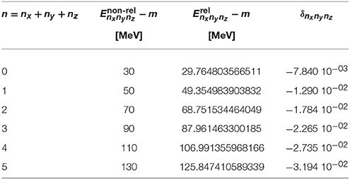
Table 1. Energies of the lowest eigenstates of a spherically symmetric harmonic oscillator with -hω = 20 MeV and m = 938 MeV/c2 in the non-relativistic and relativistic case and relative difference (87).
In general, numerical solutions of the Dirac equation depend on the deformation parameter d and three parameters that define the Lagrange-mesh method: the scale parameter h, the number of zeroes N of the Laguerre polynomial in (24) and (25), and the number of channels Nc in the expansion of the wave function as in (55). As baseline for the following calculations and comparisons, the values h = 0.1 fm, N = 25, and Nc = 11 are chosen. Because the coupling potential has positive parity, there are two distinct sequences of κ values in the expansion (47) of the single-particle state that do not couple as discussed in section 3.2. They are {1, −2, 3, −4, …} and {−1, 2, −3, 4, …} for states of positive and negative parity, respectively. From these sets Nc consecutive values κ1, …, κNc are chosen as the considered channels with the lowest value |κ1| = |Ω|+1/2. In Tables 2, 3, the exact energies of the deformed relativistic harmonic oscillator with deformation parameters d = 0.1 and d = −0.1, respectively, are given for the lowest states with nx+ny+nz ≤ 3. The corresponding parities π, principal quantum numbers n, and angular momentum projections Ω are also shown. A degeneracy of states with identical values for nx+ny and nz is clearly seen because of the rotational symmetry around the z axis. The last column in Tables 2, 3 gives the absolute deviations
of the energies , which were determined with the Lagrange-mesh method using the baseline parameters, from the exact values , which are shown in the next-to-last column. The highest accuracy is found for the states of lowest energy. It decreases with increasing principal quantum number n for fixed |Ω| and π. Nevertheless, the level of accuracy is impressive as the absolute scale of the energies in the eigenvalue problem is given by the mass m, i.e., of the order of 1 GeV.
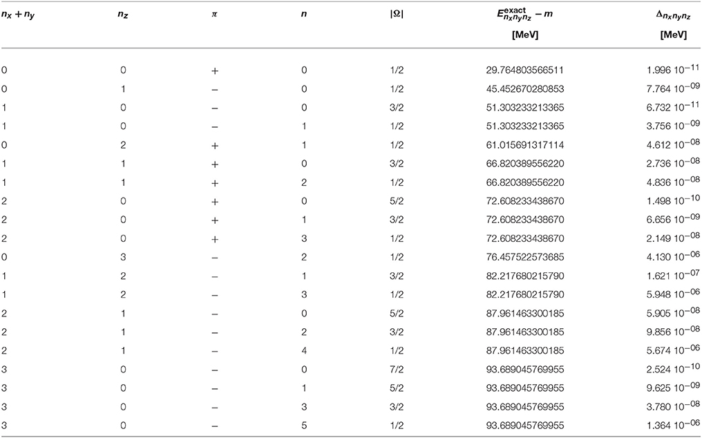
Table 2. Exact energies of the eigenstates of a prolate relativistic harmonic oscillator with d = 0.1, -hω = 20 MeV, and m = 938 MeV/c2 and absolute deviation (88) of a calculation using the Lagrange-mesh method with scaling factor h = 0.1 fm, number of grid points N = 25, and number of channels Nc = 11.
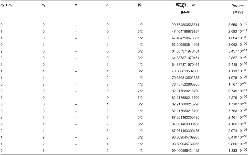
Table 3. Exact energies of the eigenstates of an oblate relativistic harmonic oscillator with d = −0.1, -hω = 20 MeV, and m = 938 MeV/c2 and absolute deviation (88) of a calculation using the Lagrange-mesh method with scaling factor h = 0.1 fm, number of grid points N = 25, and number of channels Nc = 11.
The dependence of the accuracy of the calculation on the parameters h, N, and Nc will be studied in the following sections. The parameters h and N are specific to the Lagrange-mesh method since they define the position of the discretization points for the radius. In contrast, the parameter Nc appears only because a partial-wave expansion of the three-dimensional wave fuctions was introduced in the present work. Hence, the convergence with respect to h and N is rather independent from that of Nc. Alternatively, different versions of the Lagrange-mesh method based on other basis functions using cylindrical or Cartesian coordinates could be used.
4.1.1. Variation of the Scale Parameter
The scale parameter h connects the radial grid points in a given channel κ with α = 2|κ| to the zeroes of the Laguerre polynomial . It has to be selected so that the details and the gross structure of the wave functions can be well represented. The effect of changing h can be clearly demonstrated by looking at the radial wave function of the ground and first excited state with orbital angular momentum l = 0 of a spherical relativistic harmonic oscillator. They are depicted in the left and right panel of Figure 1, respectively. In this case, only a single channel with κ = 1 has to be considered and the matrix Hamiltonian in (55) has dimension 2N × 2N with N = 25 radial grid points. The exact result for the upper component is given by a simple Gaussian φ(r) = [2/(π1/4b3/2)]exp[−r2/(2b2)] for the ground state and φ(r) = (3/2−r2/b2)[23/2/(31/2π1/4b3/2)]exp[−r2/(2b2)] for the first excited state with oscillator parameter b. Of course, the choice of Lagrange-mesh functions (20) with an exponential decay for large radii is not very well adapted to represent Gaussian-type functions and some deviation can be expected. In Figure 1, the modulus |Cφ(r)| of the exact and numerically determined wave functions are depicted. The factor C is determined such that the radial wave function of the upper component is normalized to one. Hence C = 1 for the exact result and C = [∫dr r2|φ(r)|2]−1/2 with φ(r) = Fκ(r)/r in case of the numerical calculation. For small radii r, the exact wave function (full line) practically coincides with the numerically determined wave function if the scale parameter h varies between 0.05 fm and 0.80 fm. Deviations show up for radii larger than approximately 4 fm if h = 0.05 (red squares). This fact is not surprising because the highest grid point is located at fm in this case and the Gaussian decrease of the exact wave function cannot be described well with the asymptotic form of the Lagrange-mesh functions. For h = 0.10 fm, the exact wave function is very well reproduced up to about 9.5 fm in the calculation (green circles) with a value of about 10−10 fm−3/2 for the ground state and 10−9 fm−3/2 for the first excited state, much smaller than that at the center. For larger values of h, the tail of the wave function develops an oscillatory behavior indicating that the location of the grid points is not chosen properly and the number of grid points within the major part of the wave function is too small. For example the highest grid point is at a radius of approximately 71.2 fm for h = 0.8 fm, much above the relevant range, and there are 15 points beyond 10 fm, leaving only 10 points for the region of lower radii since N = 25 in the baseline case. The tails of the wave functions of the ground and first excited state show a very similar pattern, except that the values of the excited state are about one to two order of magnitude larger. In addition, the node in this wave function is clearly visible.
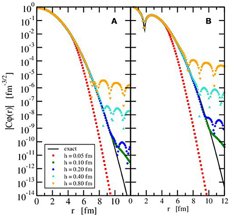
Figure 1. Modulus of the scaled radial wave function of the ground (A) and first excited (B) state with orbital angular momentum l = 0 in a spherically symmetric relativistic harmonic oscillator with ℏω = 20 MeV and m = 938 MeV/c2 in the exact case (full black line) and the calculation with the Lagrange-mesh method for different scale parameters h (colored symbols) and constant number of grid points (N = 25). The normalization factor C is explained in the text.
The dependence on the scale parameter can also be studied by looking at the deviations (88) between the calculated energies and the exact energies. They are depicted in Figure 2 for selected values of h between 0.05 fm and 1.00 fm and deformation parameters d = 0.1, d = 0.0, and d = −0.1 in (85). Only states with nx + ny + nz ≤ 2 are considered. If h is in the range of 0.08 fm to 0.3 fm, there is almost no change in the accuracy of the calculation. Only for h values outside this interval, a deterioration is observed with stronger effects at low h. In the deformed calculations also, a systematic trend with the number of excited oscillator quanta is found. The energies of higher-excited states are less well reproduced. This is related to the fact that several channels are needed for a good representation of the wave functions; see section 4.1.3. For the spherical case, the effect is much less obvious because here a single κ channel is sufficient for the calculation.
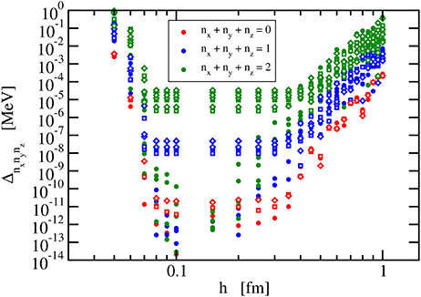
Figure 2. Deviation (88) of the calculated lowest energies of a relativistic harmonic oscillator with ℏω = 20 MeV and m = 938 MeV/c2 from the exact results for constant number of grid points (N = 25) and constant number of channels (Nc = 11). Results are shown as a function of the scaling factor h for the spherical case (full symbols), prolate deformation with d = 0.1 (open diamonds), and oblate deformation with d = −0.1 (open squares).
4.1.2. Variation of the Number of Grid Points
The choice of the order N of the Laguerre polynomial in (24) and (25) determines the number of radial grid points of the mesh. The effect of changing N can again be demonstrated by looking at the radial wave functions of the ground and excited states with l = 0 of a spherical relativistic harmonic oscillator in comparison to the exact result as in section 4.1.1. In Figure 3, the modulus |Cφ(r)| of the exact and numerically determined wave functions are depicted for constant scale parameter h = 0.1 fm varying the number of grid points. The ground and first excited states for orbital angular momentum l = 0 are considered in panels A and B, respectively. A clear improvement in the approximation of the exact wave function is found with increasing N with an increase of the radial range where the wave function is well represented. N = 10 grid points are obviously not sufficient for a good representation of the wave functions.
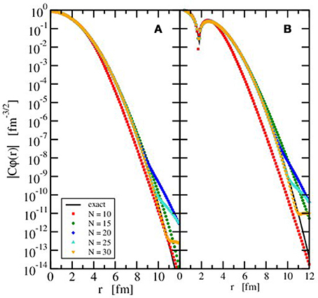
Figure 3. Modulus of the scaled radial wave function of the ground (A) and first excited (B) state with orbital angular momentum l = 0 in a spherically symmetric relativistic harmonic oscillator with ℏω = 20 MeV and m = 938 MeV/c2 in the exact case (full black line) and the calculation with the Lagrange-mesh method for different number of grid points N (colored symbols) and constant scale parameter (h = 0.10 fm). The normalization factor C is explained in the text.
Keeping h = 0.1 fm and Nc = 11 fixed, the deviations (88) of the energies are depicted in Figure 4 as a function of the number of grid points N in each channel. The deviation is largest for the lowest values of N, and no accurate results for the single-particle energies are obtained from the application of the Lagrange-mesh method. The accuracy increases with N, and above approximately N = 20, a stabilization of the deviations occurs. A further increase of the number of grid points does not result in smaller differences between exact and numerical eigenvalues.
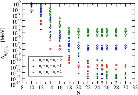
Figure 4. Deviation (88) of the calculated lowest energies of a relativistic harmonic oscillator with ℏω = 20 MeV and m = 938 MeV/c2 from the exact results for constant scaling factor (h = 0.1 fm) and constant number of channels (Nc = 11). Results are shown as a function of the number of grid points N for the spherical case (full symbols), prolate deformation with d = 0.1 (open diamonds), and oblate deformation with d = −0.1 (open squares).
4.1.3. Variation of the Number of Channels
The third parameter that is relevant in the application of the Lagrange-mesh method is the number of channels Nc in the expansion of the single-particle wave function (47). In Figure 5, the deviations (88) of the energies of the lowest states are shown for values of Nc ranging from 4 to 14. As in Figures 2, 4, the relativistic harmonic oscillator with parameters ℏω = 20 MeV and m = 938 MeV/c2 is chosen as test case with the baseline values for h and N. The spherical harmonic oscillator displays no dependence of Δnxnynz on Nc because there is no coupling between different κ channels and the accuracy of the calculation only depends on h and N as discussed in sections 4.1.1 and 4.1.2. In contrast to this case, the accuracy of the single-particle energies exhibits a clear trend of improvement with increasing number of channels in the calculations for harmonic oscillator potentials with prolate and oblate deformations. The ground state energy seems to converge for Nc reaching the baseline value but an even larger number of channels are required to obtain a similar accuracy in the calculation of excited states.
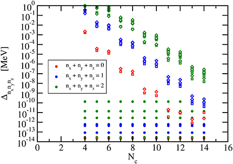
Figure 5. Deviation (88) of the calculated lowest energies of a relativistic harmonic oscillator with ℏω = 20 MeV and m = 938 MeV/c2 from the exact results for constant scaling factor (h = 0.1 fm) and constant number of grid points (N = 25). Results are shown as a function of the number of channels Nc for the spherical case (full symbols), prolate deformation with d = 0.1 (open diamonds), and oblate deformation with d = −0.1 (open squares).
4.2. Deformed Nuclei
In the description of nuclei that employs a relativistic EDF, two coupled problems have to be solved self-consistently. The single-particle wave functions of the nucleons are found as solutions of the Dirac Equation (12) with vector and scalar potentials that are determined by the meson and electromagnetic fields. These are calculated with the help of the field Equations (7)–(11) from the source densities (4) and (5) that in turn depend on the single-particle wave functions. An iterative approach is usually selected with a predefined accuracy that has to be reached for some quantities.
In the present application, the numerical methods of section 3 for the description in spherical coordinates are employed. The iteration of the coupled equations is stopped when the single-particle energies of the occupied levels do not change more than 10−6 MeV in consecutive steps. The number of grid points N in the Lagrange-mesh method and the number of channels Nc are set to the baseline values, i.e., N = 25 and Nc = 11. In contrast, the scale parameter h changes from nucleus to nucleus. With the radius estimate R = 1.2·A1/3 fm for a nucleus with mass number A and the largest zero for the Laguerre polynomial with α = 0, the scale parameter is defined as with . This choice provides a suitable discretization of the wave functions and densities in the range that is relevant for the calculation including the asymptotic behavior at large radii. Since a defined parity is imposed on the single-particle wave functions, only even angular momenta appear in the expansions of potentials (49), densities (59), fields, and sources (63). Other possibilities, e.g., octupole distributions, that would require to include odd angular momenta, are not considered here.
The EDF selected in this work is based on a relativistic mean-field model with density-dependent meson-nucleon couplings [17]. It has been applied successfully with different parametrizations in the description of nuclear structure and nuclear matter. Here, the parameter set DD2 [51] is used; this includes σ, ω, and ρ but not δ mesons to describe the effective interaction. The masses of neutrons and protons are fixed to mn = 939.565379 MeV/c2 and mp = 938.272046 MeV/c2, respectively. The nuclear matter parameters calculated with this parametrization are very reasonable and consistent with present constraints [52].
As examples for the application of the Lagrange-mesh method, the ground states of self-conjugate even-even nuclei from 4He to 40Ca are calculated with mass numbers that are multiples of four. They show large structural differences and the nucleon distribution changes between spherical, oblate, and prolate shapes. The rather small number of nucleons allows a fast calculation and the choice of the baseline parameters N = 25 and Nc = 11 in the Lagrange-mesh method is sufficient to obtain faithful results. It is expected that the exponential decrease of the radial Lagrange-mesh functions gives a better approximation of the single-particle wave functions in a nucleus than in a harmonic oscillator. The obtained accuracy is fully adequate for a representation of single-particle energies and density distributions in the manner of the figures in this work. The matter radii and deformation parameters are expected to change at most by one unit in the last digit given in Table 4 if the precision is improved by increasing the number channels Nc as trial calculations have shown.
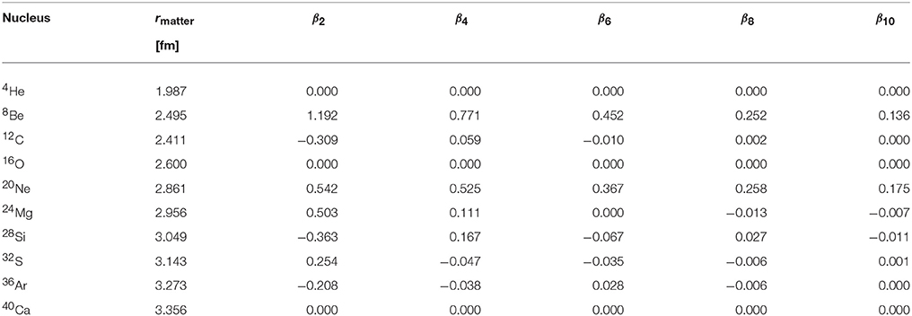
Table 4. Point matter radius rmatter and deformation parameters β2, …, β10 for nuclei 4He, …, 40Ca.
In Figures 6, 7, the single-particle energies of neutrons and protons are shown, respectively. Each circle represents a pair of states (n, π, Ω) and (n, π, −Ω). Degenerate levels are clearly identified in the spherical closed-shell nuclei 4He, 16O, and 40Ca where the orbital angular momentum is an additional good quantum number that characterizes a level. These levels belong to p, d, and f states. There is no such degeneracy found in the remaining deformed nuclei. Owing to the Coulomb repulsion, the proton levels are less bound than the neutron levels with increasing charge number of the nucleus. Shell gaps are easily identified, in particular, for the less strongly deformed nuclei.
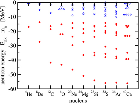
Figure 6. Neutron levels in the self-conjugated even-even nuclei 4He - 40Ca. Occupied levels (with two neutrons) are denoted by a full red circle and unoccupied levels by an open blue circle.
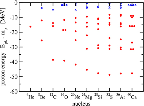
Figure 7. Proton levels in the self-conjugated even-even nuclei 4He - 40Ca. Occupied levels (with two protons) are denoted by a full red circle and unoccupied levels by an open blue circle.
The main observable considered here is the point nuclear matter distribution in the intrinsic frame of the nucleus. It is obtained by adding the vector densities as given in (59) of all occupied single-particle states. This intrinsic density depends on the three Cartesian coordinates xyz in the body-fixed frame of the nucleus. The nuclear matter distributions in the laboratory frame, obtained from a projection on good total angular momentum J, would be spherical since only even-even nuclei in their ground state with J = 0 are considered here. Instead of showing radial density distributions that would depend on the the polar angle, intrinsic matter distributions are depicted for all 10 nuclei in Figures 8–11 using lines of constant density in the xz plane to show the deformation clearly. Owing to the axial symmetry, the density distributions are invariant for a rotation around the z axis and hence the lines of constant density in the yz plane would look identical to those in the xz plane or any plane that contains the z axis. As expected for doubly-magic nuclei, 4He, 16O, and 40Ca are spherically symmetric. In the case of 4He and 40Ca, the maximum density is at the center of the nucleus, whereas 16O exhibits a central depression; see Figure 9. The nuclei 8Be, 20Ne, 24Mg, and 32S show a prolate point matter distribution, however, with distinct differences. A pronounced two-alpha cluster structure is visible in 8Be. A pronounced bulge in the xy plane is found in 20Ne but not in 24Mg. The prolate deformation is less obvious for 32S and the density maxima lie even in the xy plane and not on the z axis as for the other prolate nuclei. An oblate density distribution of the ground state is predicted for 12C, 28Si, and 36Ar. A bulge along the z axis is obtained for 28Si and density maxima on this symmetry axis are seen for 36Ar in contrast to 12C and 28Si. Looking at the sequence of nuclei with increasing A, an increasing extension of the density distribution can be also traced that will be reflected in the matter root-mean-square radius.
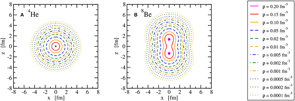
Figure 8. Lines of constant intrinsic matter density ρ of the nuclei 4He (A) and 8Be (B). Points of maximum density are indicated with a × .
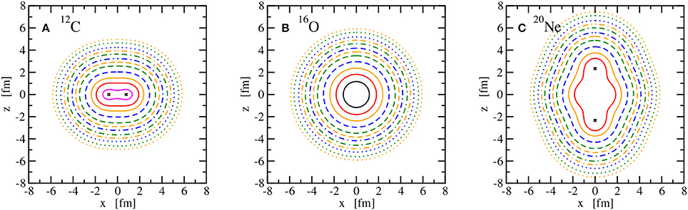
Figure 9. Lines of constant intrinsic matter density ρ of the nuclei 12C (A), 16O (B), and 20Ne (C). See Figure 8 for the legend. Points of maximum density are indicated with a × or a full black line in case of 16O.
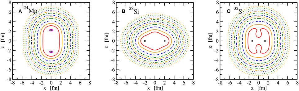
Figure 10. Lines of constant intrinsic matter density ρ of the nuclei 24Mg (A), 28Si (B), and 32S (C). See Figure 8 for the legend. Points of maximum density are indicated with a × .
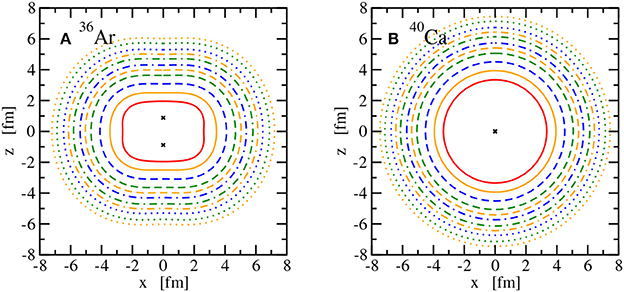
Figure 11. Lines of constant intrinsic matter density ρ of the nuclei 36Ar (A) and 40Ca (B). See Figure 8 for the legend. Points of maximum density are indicated with a × .
In Table 4, the point matter root-mean-square radii rmatter of the nuclei are explicitly given in the second column. They are calculated as
with the vector densities (2) of neutrons and protons. The radii rmatter increase with the mass number A except for the step from A = 8 to A = 12 because the nucleus 8Be has a particular large radius due to the pronounced cluster structure with two α particles. In reality, 8Be is even unbound for the decay into two 4He. It is only a resonance in this channel at an energy of 91.84 keV [53]. Besides the point matter radii, Table 4 also gives the deformation parameters βL for L = 0, 2, 4, 6, 8, and 10. They are defined as
with factors A and R in the denominator to obtain a dimensionless quantity that is approximately independent of the size of the nucleus and thus comparable between different nuclei. The radius estimate R = 1.2·A1/3 fm is defined as above in the determination of the scale parameter h. The value of βL for all L vanishes for the spherical nuclei 4He, 16O, and 40Ca. Prolate nuclei have a positive β2 and oblate nuclei have a negative β2 but the signs of βL with L > 2 are not strictly correlated with the occurrence of a prolate or oblate deformation. The moduli of the deformation parameters usually become smaller with increasing L. The decrease is fast in the case of 12C, 32S, and 36Ar where higher-order deviations from a quadrupole distribution are not very significant. 28Si is an intermediate case and the most extreme variation of the distribution is found for 8Be and 20Ne. Substantial values of βL for large L indicate that channels with large differences of the κ values couple strongly in the diagonalization of the single-nucleon Dirac Hamiltonian. Hence a large number of channels is required for the convergence of the results.
Binding energies of the nuclei are not given here since the energy (16) has to be corrected by a proper projection on center-of-mass momentum and specific total angular momentum or by applying approximate treatments. Methods to perform these corrections will be discussed elsewhere. The angular momentum projection will profit from the representation of the single-particle wave functions in spherical coordinates as proposed in this work.
5. Conclusion
The Lagrange-mesh method is a very efficient variational approach to solve differential equations numerically with high precision. It has been used extensively in non-relativistic problems but in this work it has been formulated for the application to the Dirac equation to find bound states of fermions moving in deformed but axially symmetric potentials. This problem appears in the description of nuclei employing relativistic energy density functionals. The use of spherical coordinates leads to an eigenvalue problem with coupled equations of the radial wave functions. They are expanded in a set of Lagrange-mesh functions derived from Laguerre polynomials. Finally, a Hamiltonian matrix of moderate size has to be diagonalized.
The accuracy of the Lagrange-mesh method depends on three parameters: the scale factor, the number of grid points, and the number of channels. The dependence of the numerical precision on these parameters was studied by comparing analytical solutions for a deformed relativistic harmonic oscillator potential with numerical results obtained with the proposed formulation of the Lagrange-mesh method. With appropriate choices of the parameters, very accurate solutions are found without extensive computational efforts.
The description of ground states of self-conjugated even-even nuclei from 4He to 40Ca was chosen as an application of the Lagrange-mesh method to a problem in nuclear structure physics. The equations of motion of nucleons, mesons, and the electromagnetic field were derived from a relativistic energy density functional based on a relativistic mean-field approach with density-dependent nucleon-meson couplings. The field equations were solved self-consistently by iteration, yielding the single-particle states of the nucleons and the intrinsic density distributions. A strong variation of the shapes and deformation parameters is found with spherical, oblate, and prolate distributions.
The present work focused on formulating the basic application of the Lagrange-mesh method to relativistic nuclear structure calculations. The presented approach can be extended easily in the future. The restriction to intrinsic states of given parity can be lifted allowing, e.g., also the description of octupole deformations. Proper projections, e.g., on given angular momentum and parity, are needed for a comparison of densities, radii, and energies with experimental data. Constraints on different multipole moments can be introduced and beyond mean-field calculations, e.g., using the generator-coordinate approach, are foreseeable.
Author Contributions
ST wrote and tested the computer program, performed all calculations, prepared the tables and figures, and wrote the manuscript.
Funding
This work was partly supported by the Deutsche Forschungsgemeinschaft (DFG) through grant no. SFB 1245.
Conflict of Interest Statement
The author declares that the research was conducted in the absence of any commercial or financial relationships that could be construed as a potential conflict of interest.
References
1. Bender, M, Heenen, PH, and Reinhard, PG Self-consistent mean-field models for nuclear structure. Rev Mod Phys. (2003) 75:121–80. doi: 10.1103/RevModPhys.75.121
2. Serot, BD, and Walecka, JD The relativistic nuclear many body problem. Adv Nucl Phys. (1986) 16:1–327.
3. Ring, P Relativistic mean field in finite nuclei. Prog Part Nucl Phys. (1996) 37:193–263. doi: 10.1016/0146-6410(96)00054-3
4. Serot, BD, and Walecka, JD Recent progress in quantum hadrodynamics. Int J Mod Phys. (1997) E6:515–631. doi: 10.1142/S0218301397000299
5. Lalazissis, GA, Ring, P, and Vretenar, D Extended Density Functionals in Nuclear Structure Physics. Lecture Notes in Physics 641. Berlin; Heidelberg: Springer (2004).
6. Vretenar, D, Afanasjev, AV, Lalazissis, GA, and Ring, P Relativistic Hartree Bogoliubov theory: static and dynamic aspects of exotic nuclear structure. Phys Rept. (2005) 409:101–259. doi: 10.1016/j.physrep.2004.10.001
7. Meng, J, Toki, H, Zhou, SG, Zhang, SQ, Long, WH, and Geng, LS Relativistic Continuum Hartree Bogoliubov theory for ground state properties of exotic nuclei. Prog Part Nucl Phys. (2006) 57:470–563. doi: 10.1016/j.ppnp.2005.06.001
8. Nikšić, T, Vretenar, D, and Ring, P Relativistic nuclear energy density functionals: mean-field and beyond. Prog Part Nucl Phys. (2011) 66:519–48. doi: 10.1016/j.ppnp.2011.01.055
9. Ring, P, Abusara, H, Afanasjev, AV, Lalazissis, GA, Nikšić, T, and Vretenar, D Modern applications of covariant density functional theory. Int J Mod Phys. (2011) E20:253. doi: 10.1142/S0218301311017570
10. Horowitz, CJ, and Serot, BD Selfconsistent Hartree description of finite nuclei in a relativistic quantum field theory. Nucl Phys. (1981) A368:503–28. doi: 10.1016/0375-9474(81)90770-3
11. Bonche, P, Flocard, H, Heenen, PH, Krieger, SJ, and Weiss, MS Self-consistent study of triaxial deformations: application to the isotopes of Kr, Sr, Zr and Mo. Nucl Phys. (1985) A443:39–63. doi: 10.1016/0375-9474(85)90320-3
12. Reinhard, PG, Rufa, M, Maruhn, J, Greiner, W, and Friedrich, J Nuclear ground state properties in a relativistic meson field theory. Z Phys. (1986) A323:13–25. doi: 10.1007/BF01294551
13. Pöschl, W, Vretenar, D, Rummel, A, and Ring, P Application of finite element methods in relativistic mean-field theory: spherical nucleus. Comp Phys Commun. (1997) 101:75–107. doi: 10.1016/S0010-4655(97)84583-3
14. Pöschl, W, Vretenar, D, and Ring, P Relativistic Hartree-Bogoliubov theory in coordinate space: finite element solution for a nuclear system with spherical symmetry. Comp Phys Commun. (1997) 103:217–50. doi: 10.1016/S0010-4655(97)00042-8
15. Meng, J Relativistic continuum Hartree-Bogoliubov theory with both zero range and finite range Gogny force and their application. Nucl Phys. (1998) A635:3–42. doi: 10.1016/S0375-9474(98)00178-X
16. Stoitsov, M, Ring, P, Vretenar, D, and Lalazissis, GA Solution of relativistic Hartree-Bogolyubov equations in configurational representation: spherical neutron halo nuclei. Phys Rev. (1998) C58:2086–91.
17. Typel, S, and Wolter, HH Relativistic mean field calculations with density dependent meson nucleon coupling. Nucl Phys. (1999) A656:331–64. doi: 10.1016/S0375-9474(99)00310-3
18. Gambhir, YK, Ring, P, and Thimet, A Relativistic mean field theory for finite nuclei. Ann Phys. (1990) 198:132–79. doi: 10.1016/0003-4916(90)90330-Q
19. Ring, P, Gambhir, YK, and Lalazissis, GA Computer program for the relativistic mean field description of the ground state properties of even-even axially deformed nuclei. Comp Phys Commun. (1997) 105:77–97. doi: 10.1016/S0010-4655(97)00022-2
20. Zhou, SG, Meng, J, and Ring, P Spherical relativistic Hartree theory in a Woods-Saxon basis. Phys Rev. (2003) C68:034323. doi: 10.1103/PhysRevC.68.034323
21. Nikšić, T, Vretenar, D, Tian, Y, Ma, Zy, and Ring, P 3D Relativistic Hartree-Bogoliubov model with a separable pairing interaction. Phys Rev. (2010) C81:054318. doi: 10.1103/PhysRevC.81.054318
22. Nikšić, T, Paar, N, Vretenar, D, and Ring, P DIRHB - A relativistic self-consistent mean-field framework for atomic nuclei. Comput Phys Commun. (2014) 185:1808–21. doi: 10.1016/j.cpc.2014.02.027
23. Umar, AS, Strayer, MR, Wu, JS, Dean, DJ, and Guclu, MC Nuclear Hartree-Fock calculations with splines. Phys Rev. (1991) C44:2512–21. doi: 10.1103/PhysRevC.44.2512
24. Pei, JC, Stoitsov, MV, Fann, GI, Nazarewicz, W, Schunck, N, and Xu, FR Deformed coordinate-space Hartree-Fock-Bogoliubov approach to weakly bound nuclei and large deformations. Phys Rev. (2008) C78:064306. doi: 10.1103/PhysRevC.78.064306
25. Pei, JC, Kortelainen, M, Zhang, YN, and Xu, FR Emergent soft monopole modes in weakly-bound deformed nuclei. Phys Rev. (2014) C90:051304. doi: 10.1103/PhysRevC.90.051304
26. Davies, KTR, Flocard, H, Krieger, S, and Weiss, MS Application of the imaginary time step method to the solution of the static Hartree-Fock problem. Nucl Phys. (1980) A342:111–23. doi: 10.1016/0375-9474(80)90509-6
27. Reinhard, PG, and Cusson, RY A comparative study of Hartree-Fock iteration techniques. Nucl Phys. (1982) A378:418–42. doi: 10.1016/0375-9474(82)90458-4
28. Ryssens, W, Hellemans, V, Bender, M, and Heenen, PH Solution of the SkyrmeHF+BCS equation on a 3D mesh, II: a new version of the Ev8 code. Comput Phys Commun. (2015) 187:175–94. doi: 10.1016/j.cpc.2014.10.001
29. Maruhn, JA, Reinhard, PG, Stevenson, PD, and Umar, AS The TDHF code Sky3D. Comput Phys Commun. (2014) 185:2195–216. doi: 10.1016/j.cpc.2014.04.008
30. Schunck, N, McDonnell, JD, Sarich, J, Wild, SM, and Higdon, D Error analysis in nuclear density functional theory. J Phys. (2015) G42:034024. doi: 10.1088/0954-3899/42/3/034024
31. Rodríguez, TR, Arzhanov, A, and Martínez-Pinedo, G Toward global beyond-mean-field calculations of nuclear masses and low-energy spectra. Phys Rev. (2015) C91:044315. doi: 10.1103/PhysRevC.91.044315
32. Tanimura, Y, Hagino, K, and Liang, HZ 3D mesh calculations for covariant density functional theory. PTEP (2015) 2015:073D01. doi: 10.1093/ptep/ptv083
33. Baye, D, and Heenen, PH Generalised meshes for quantum mechanical problems. J Phys A Math Gen. (1986) 19:2041. doi: 10.1088/0305-4470/19/11/013
34. Baye, D, Hesse, M, and Vincke, M The unexplained accuracy of the Lagrange-mesh method. Phys Rev E (2002) 65:026701. doi: 10.1103/PhysRevE.65.026701
35. Imagawa, H, and Hashimoto, Y Accurate random phase approximation calculation of low lying states on a three-dimensional Cartesian mesh. Phys Rev. (2003) C67:037302. doi: 10.1103/PhysRevC.67.037302
36. Hashimoto, Y Time-dependent Hartree-Fock-Bogoliubov calculations using a Lagrange mesh with the Gogny interaction. Phys Rev. (2013) C88:034307. doi: 10.1103/PhysRevC.88.034307
37. Baye, D The Lagrange-mesh method. Phys Rep. (2015) 565:1–107. doi: 10.1016/j.physrep.2014.11.006
38. Baye, D, Filippin, L, and Godefroid, M Accurate solution of the Dirac equation on Lagrange meshes. Phys Rev E (2014) 89:043305. doi: 10.1103/PhysRevE.89.043305
39. Filippin, L, Godefroid, M, and Baye, D Relativistic polarizabilities with the Lagrange-mesh method. Phys Rev A (2014) 90:052520. doi: 10.1103/PhysRevA.90.052520
40. Mohr, PJ, Newell, DB, and Taylor, BN CODATA recommended values of the fundamental physical constants: 2014. Rev Mod Phys. (2016) 88:035009. doi: 10.1103/RevModPhys.88.035009
41. Typel, S Relativistic mean-field models with different parametrizations of density dependent couplings. Particles (2018) 1:1. doi: 10.3390/particles1010002
42. Abramowitz, M, and Stegun, IA Handbook of Mathematical Functions with Formulas, Graphs, and Mathematical Tables. New York, NY: Dover Publications, Inc. (1965).
43. Press, WH, Flannery, BP, Teukolsky, SA, and Vetterling, WT Numerical Recipes. Cambridge: Cambridge University Press (1987).
44. Lisboa, R, Malheiro, M, de, Castro AS, Alberto, P, and Fiolhais, M Pseudospin symmetry and the relativistic harmonic oscillator. Phys Rev. (2004) C69:024319. doi: 10.1103/PhysRevC.69.024319
45. Ginocchio, JN U(3) and pseudo-U(3) symmetry of the relativistic harmonic oscillator. Phys Rev Lett. (2005) 95:252501. doi: 10.1103/PhysRevLett.95.252501
46. Guo, JY, Fang, XZ, and Xu, FX Pseudospin symmetry in the relativistic harmonic oscillator. Nucl Phys. (2005) A757:411–21. doi: 10.1016/j.nuclphysa.2005.04.017
47. de, Castro AS, Alberto, P, Lisboa, R, and Malheiro, M Relating pseudospin and spin symmetries through charge conjugation and chiral transformations: the case of the relativistic harmonic oscillator. Phys Rev. (2006) C73:054309. doi: 10.1103/PhysRevC.73.054309
48. Ikeda, K, Takigawa, N, and Horiuchi, H The systematic structure-change into the molecule-like structures in the self-conjugate 4n nuclei. Prog Theor Phys Suppl. (1968) E68:464–75. doi: 10.1143/PTPS.E68.464
49. Tohsaki, A, Horiuchi, H, Schuck, P, and Röpke, G Alpha cluster condensation in C-12 and O-16. Phys Rev Lett. (2001) 87:192501. doi: 10.1103/PhysRevLett.87.192501
50. Girod, M, and Schuck, P α-particle clustering from expanding self-conjugate nuclei within the Hartree-Fock-Bogoliubov approach. Phys Rev Lett. (2013) 111:132503. doi: 10.1103/PhysRevLett.111.132503
51. Typel, S, Röpke, G, Klähn, T, Blaschke, D, and Wolter, HH Composition and thermodynamics of nuclear matter with light clusters. Phys Rev. (2010) C81:015803. doi: 10.1103/PhysRevC.81.015803
52. Dutra, M, Lourenço, O, Avancini, SS, Carlson, BV, Delfino, A, Menezes, DP, et al. Relativistic mean-field hadronic models under nuclear matter constraints. Phys Rev. (2014) C90:055203. doi: 10.1103/PhysRevC.90.055203
Keywords: Lagrange-mesh method, relativistic energy density functional, density-dependent couplings, deformed nuclei, relativistic harmonic oscillator, Dirac equation
Citation: Typel S (2018) Lagrange-Mesh Method for Deformed Nuclei With Relativistic Energy Density Functionals. Front. Phys. 6:73. doi: 10.3389/fphy.2018.00073
Received: 26 April 2018; Accepted: 26 July 2018;
Published: 06 August 2018.
Edited by:
Isaac Vidana, Istituto Nazionale di Fisica Nucleare (INFN), ItalyReviewed by:
Constança Providência, University of Coimbra, PortugalPierre Descouvemont, Free University of Brussels, Belgium
Copyright © 2018 Typel. This is an open-access article distributed under the terms of the Creative Commons Attribution License (CC BY). The use, distribution or reproduction in other forums is permitted, provided the original author(s) and the copyright owner(s) are credited and that the original publication in this journal is cited, in accordance with accepted academic practice. No use, distribution or reproduction is permitted which does not comply with these terms.
*Correspondence: Stefan Typel, s.typel@gsi.de