Spatiotemporal Permutation Entropy as a Measure for Complexity of Cardiac Arrhythmia

Permutation entropy (PE) is a robust quantity for measuring the complexity of time series. In the cardiac community it is predominantly used in the context of electrocardiogram (ECG) signal analysis for diagnoses and predictions with a major application found in heart rate variability parameters. In this article we are combining spatial and temporal PE to form a spatiotemporal PE that captures both, complexity of spatial structures and temporal complexity at the same time. We demonstrate that the spatiotemporal PE (STPE) quantifies complexity using two datasets from simulated cardiac arrhythmia and compare it to phase singularity analysis and spatial PE (SPE). These datasets simulate ventricular fibrillation (VF) on a two-dimensional and a three-dimensional medium using the Fenton-Karma model. We show that SPE and STPE are robust against noise and demonstrate its usefulness for extracting complexity features at different spatial scales.

1. Introduction

A healthy heart is driven by periodic plane waves propagating over the cardiac tissue. These waves can turn into potentially life-threatening self-sustained arrhythmias which are governed by reentrant spiral-wave activity of different levels of complexity [1, 2].

A detailed understanding of the complexity of cardiac arrhythmias and the organization of spiral-wave activity is crucial for the development of improved methods for the treatment of cardiac arrhythmias [3–5].

In the healthy sinus rhythm a lot of information about the state of the heart is already contained in the frequency and timings of individual heartbeats. Furthermore, the ECG is one of the most important clinical tools for the identification of deviations from the normal rhythm and is prevalently used for medical diagnoses. In case of cardiac arrhythmias with a spatiotemporally more unordered state, measures that allow for a quantification of the spatiotemporal complexity of the system provide valuable information that can be used for investigating the mechanisms behind the onset of arrhythmia and their possible termination.

In the picture of an arrhythmia being composed of many interacting spiral waves or three-dimensional rotors, often the concept of phase singularities is used to assess the degree of organization. A high number of phase singularities (NPS) corresponds to a state with more rotors and therefore indicates a situation with higher complexity. However, in experimental situations where usually surface electric activity of the heart is measured by optical mapping using fluorescent dyes, several practical problems arise:

• As only two-dimensional information of a three-dimensional medium is recorded, phenomena on the surface can not always be suitably approximated by the concept of phase singularities. For example, focal activity on the surface, which can be produced by spirals located far away from the surface, would not be covered by NPS.

• Noise can significantly impair the detection of phase singularities, so usually the application of spatial kernel-smoothing and temporal bandapass filters is required.

• Usually high-level algorithms for a reliable computation of NPS involve sophisticated tracking algorithms for phase singularities over time. These methods can be computationally intensive and prevent real-time applications.

To tackle these problems other suitable methods for characterizing and quantifying spatiotemporal complexity are desired. In this article we show how a spatial and a spatiotemporal version of PE can be used to accomplish this task.

Permutation entropy (PE, [6]) is a measure which is widely used to analyse the complexity of time series signals. In the cardiac community it is so far mainly used for analysis of ECG signals, especially for the analysis of heart rate variability [7]. The concept has already been extended to two-dimensional patterns [8] and applied to optical imaging of cardiac cell culture [9].

Furthermore, its robustness against noise and the possibility to study complexity on different scales will be subject to this study. As our main motivation for the investigation of these methods is their potential application in experiments, we frame this numeric comparison to a realistic experimental setting: As will be explained in section 2.6 a dataset from a three-dimensional Fenton-Karma simulation is used to generate “artificial camera data”. This means that we use four two-dimensional projections of the three-dimensional simulations to approximate an experimental camera setup. Additionally, we use an algorithm for computing NPS which can also be employed for experimental data. This algorithm is presented in section 2.5 and makes use of some improved strategies to reliably detect and track spiral waves on experimental cardiac tissue.

2. Methods

This section will explain the concept of spatial and spatiotemporal PE. It also intruduces a specialized algorithm for tracking phase singularities which is used for comparison with the permutation entropy based complexity measures. Section 2.6 describes the simulations that were used to create the two numerical datasets which are subject of this investigation.

2.1. Permutation Entropy (PE)

PE [6, 7, 10] is a method for quantifying the complexity of a time series using the distribution of order patterns. Order patterns are small segments of time series of length D which are characterized solely by the relative order of their constituents. The segments, also called words $\widetilde{w_i}=w_{i,1},\dots ,w_{i,D}$ of length D, are extracted from the original time series x₁, x₂, …, x_N by taking successive elements x_i which can be separated by a time delay or lag L_t: $\widetilde{w_i}=x_i,x_{i+L_t},x_{i+2L_t},\dots ,x_{i+(D-1)L_t}$. Using these words the original time series can be transformed into a symbolic time series {s_i} by computing the permutation index that quantifies the relative order of the w_{i, j}:

$\begin{array}{ll}{s}_i={\displaystyle \sum _{j=1}^{D-1}(D-j)}!{\lambda }_{i,j}& (1)\end{array}$

$\begin{array}{ll}{\lambda }_{i,j}={\displaystyle \sum _{k=j+1}^D\{\begin{array}{ll}1\hfill & \text{if} w_{i,j}<w_{i,k}\hfill \\ 0\hfill & \text{else}\hfill \end{array}}& (2)\end{array}$

This procedure is illustrated in Figure 1A for D = 3 and L_t = 1. PE is then defined as the Shannon entropy of the relative frequencies p_j, j ∈ {1, …, D!} of the symbols s_i within the time series:

$\begin{array}{ll}\begin{array}{l}H=-{\displaystyle \sum _{j=1}^{D!}{p}_j}{\log }_2{p}_j\hfill \end{array}& (3)\end{array}$

2.2. Spatial Permutation Entropy (SPE)

The two-dimensional extension of PE which we call SPE is similar to Ribeiro et al. [8] and has been previously applied to optical mapping data of cardiac cell culture in Schlemmer et al. [9]. For SPE symbols are extracted from two-dimensional images as depicted in Figure 1B by sampling words ${\tilde{w}}_{i_1,i_2}$ of length D × D from the two dimensional data $M\in {ℝ}^{n_1\times n_2}$

$\begin{array}{ll}\begin{array}{l}{\tilde{w}}_{i_1,i_2}=m_{i_1,i_2},m_{i_1+L_x,i_2},m_{i_1+2L_x,i_2},\dots m_{i_1+(D-1)L_x,i_2},\hfill \\ m_{i_1,i_2+L_x},\dots ,m_{i_1+(D-1)L_x,i_2+(D-1)L_x}\hfill \end{array}& (4)\end{array}$

with a spatial separation L_x which replaces the one dimensional lag. So each word contains data from a grid of D × D points which are separated in both directions by the spatial separation L_x. The number of possible symbols is (D · D)! which grows very rapidly with D. Therefore, we choose D = 2 which leads to the simplified form:

$\begin{array}{ll}\begin{array}{l}{\tilde{w}}_{i_1,i_2}=m_{i_1,i_2},m_{i_1+L_x,i_2},m_{i_1,i_2+L_x},m_{i_1+L_x,i_2+L_x}\hfill \end{array}& (5)\end{array}$

which is also shown in Figure 1B.

FIGURE 1

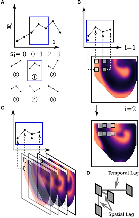
Figure 1. Construction of temporal (A), spatial (B) and spatiotemporal (C) PE. (D) Shows the tripod used for STPE. See text in sections 2.1, 2.2, 2.3 for details. (A) Shows the extraction of one-dimensional order patterns from a time series x_i and the assignment to symbols s_i. (B) Illustrates how two-dimensional order patterns are sampled from an individual image. The 2 × 2 sampling-grid is moved over all possible positions of the image. (C) Sketches how three-dimensional order patterns are extracted from subsequent images which form the video under investigation.

The grid is moved over all possible positions within the image leading to a distribution p_j of symbols s_{i1, i2} which are computed using (Equation 2). SPE is defined as the Shannon entropy (Equation 3) of this symbol distribution.

2.3. Spatiotemporal Permutation Entropy (STPE)

A natural extension of this approach to three-dimensional data can be constructed by sampling the words from volumes instead of images. This enables us to take into account spatial and temporal dimensions at the same time. It is obvious that a lot of different possibilities exist to actually sample three dimensional data points. Since the number of possible symbols grows very rapidly with the number of sampling points we restrict this approach to a “sampling tripod” which is shown in Figure 1D. The words are defined as:

$\begin{array}{ll}\begin{array}{l}{\tilde{w}}_{i_1,i_2,i_3}=v_{i_1,i_2,i_3},v_{i_1+L_x,i_2,i_3},v_{i_1,i_2+L_x,i_3},v_{i_1,i_2,i_3+L_t}\hfill \end{array}& (6)\end{array}$

where $V\in {ℝ}^{n_1,n_2,n_t}$ denotes a spatiotemporal volume with the third axis being the temporal axis. n₁ and n₂ correspond to the image size and n_t is the total number of timesteps in the video. There also exists a high flexibility in the choice of sampling parameters for the different types of separation. We chose a distinct spatial separation L_x and a different temporal separation L_t. Analogous to SPE we can again assign order patterns s_{i1, i2, i3} to the words using (Equation 2).

The procedure for extracting three-dimensional order patterns is sketched in Figure 1C. For computing the value of STPE at one timestep t all symbols s_{i1, i2, i3} from a subvolume $V_{\text{s},t}\in {ℝ}^{n_1,n_2,n_{\text{s}}}\subset V$ of the original video are taken into account to generate the distribution p_j of symbols s for this timestep and t ≤ i₃ < t + n_s. n_s can be called the window size, because it denotes the temporal size of the subvolume of the video from which the symbol distribution is taken.

In summary the STPE method in the version described here comprises three parameters:

• L_x: The spatial separation which selects the spatial scale for highlighting complexity.

• L_t: The temporal lag which specifies the temporal scale taken into account for each word.

• n_s: The window size which indicates the length of the interval analyzed by the method at a single point in time.

Scanning of all parameters has revealed that wide ranges for L_x and L_t are possible to visualize changes in complexity for all datasets analyzed here. The spatial separation L_x has been found to display some fine-grained information which will be discussed in sections 3.1, 3.4. L_t = 9 which is on the order of a short action potential has been used in all analyses here. The window size has an effect that is similar to a smoothing window size: Small n_s will take into account only very few timesteps and therefore create results similar to SPE. This usually produces strong fluctuations as the exact distribution of spatial patterns is influenced by periodic fluctuations due to finite size effects. Therefore it is usually desirable to tune n_s to a typical periodicity within the video, like a small multiple of the period of spiral rotation. If n_s is chosen too high, changes in complexity are smoothed out. We use n_s = 250 throughout this study.

It is interesting to notice, that the order in which the points are sampled from the images or volumes does not change SPE and STPE. It solely influences the assignment of the patterns to symbols, but the distribution of symbols remains the same apart from this change in labels. We used the forward construction for sampling STPE which means that one sampling point is placed at t + L_t.

2.4. Normalized Quantities

For comparing SPE and STPE obtained for different parameters, especially different L_x, it is useful to use temporally normalized versions of the quantities. The reason for this is that for larger spatial separations the spatial and spatiotemporal permutation entropies usually increase. These quantities are normalized here by subtracting the temporal mean (MEAN) and afterwards dividing by the temporal standard deviation (STD). For comparison, the normalized NPS is defined analogously. So for time series STPE, SPE and NPS we obtain the three corresponding normalized quantities as:

$\begin{array}{ll}\text{nSTPE}=\frac{\text{STPE}-\text{MEAN}(\text{STPE})}{\text{STD}(\text{STPE})}& (7)\end{array}$

$\begin{array}{ll}\text{nSPE}=\frac{\text{SPE}-\text{MEAN}(\text{SPE})}{\text{STD}(\text{SPE})}& (8)\end{array}$

$\begin{array}{ll}\text{nNPS}=\frac{\text{NPS}-\text{MEAN}(\text{NPS})}{\text{STD}(\text{NPS})}& (9)\end{array}$

2.5. Phase Singularity Tracking

Phase singularities (PS) are a widespread measure for the description of complexity of excitable media. They are found at the centers of rotation of spiral waves. In cardiac dynamics spirals and their breakup are directly related to the onset and sustaining of arrhythmias allowing for a straight-forward interpretation of PS statistics in this field of research. In this formalism every cell is assumed to undergo a phase oscillation between zero and 2π with neighboring cells typically having only a slight shift in their respective phases. In such systems points or defects where the phase is non-continuous are important features that follow certain topological laws [11].

In practice, especially with a noisy signal, PS tracking is non-trivial. Without enough smoothing an abundance of short lived PS can skew the result. Also in practice very short lived PS are often not of general interest, such as for example at the front of colliding waves, while the definition of the phase itself is not always unambiguous for high dimensional oscillators such as cardiac cells.

Unless, or even if, strong spatiotemporal smoothing is used, it is thus necessary to remove or ignore short lived PS as well as to be able to track the path of PS which can, in principle, move arbitrarily fast. Only by employing tracking reliable life times can be defined.

2.5.1. Definition of Phase

Within cardiac dynamics two main approaches for PS detection exist. One based on the definition of phases obtained from delay reconstruction [2, 12] or Hilbert transform of the signal and the other on finding of pivoting points or wave breaks based on threshold crossings [13–15]. Further improvements have been suggested for example by Rogers using wavefront tracking to improve the identification of PS [16].

The difference in these approaches lies in a slightly different phase definition. They use either a phase defined by delay embedding or the Hilbert transform, or apply threshold crossings which implicitly define a specific phase at the waves up- and downstroke. In the context of a phase defined using embedding PS are usually detected by a line integral around the current position. When using thresholds PS are naturally found at the end of lines of same phase given by the points where up- and downstroke meet. Both concepts are equivalent when interpreting the wavefront and -back each as a phase step of π.

The methodology used here is an improved detection procedure based on the aforementioned concepts. Our method is based on the idea that the upstroke is the single well and clearly defined phase, though the exact classification as such will in practice always depend on choosing some threshold. Further, we will later assume that after each upstroke the cardiac cell has a refractory period, removing the necessity of also reliably finding the APD.

After possibly preprocessing with a spatial smoothing (not done in this simulation study, see section 3.3), instead of using thresholds to identify the upstroke we use the local maximum of a correlation with a smooth upstroke-like wavelet (Figure 2B). Additionally for each pixel a threshold is set, below which a maximum is ignored, since small local maxima may arise due to noise. During this step local maxima which are very close are discarded picking the most prominent upstrokes first. An example of this procedure is shown in Figure 2. After identification the times when each upstroke occurred are stored. This is used as input for the PS identification and tracking since the time of the upstrokes defines a zero phase at the wavefront.

FIGURE 2

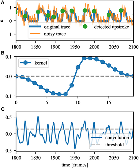
Figure 2. Sketch of the method used for defining the upstrokes. (A) The original and noisy time trace. The dots show the final times of the upstroke based on the noisy time trace. (B) The kernel which is correlated with the noisy signal in (A) to find the upstroke position. (C) Result of the correlation of the noisy signal in (A) and the kernel in (B). Local maxima identify the upstroke position (as indicated in A). A threshold is used to ignore unclear events.

2.5.2. Tracking of PS

To track PS including their exact trajectories we now make two additional assumptions. First, we assume that there exists a period of time τ during which a wavefront will have traveled at least one pixel, so a slowest reasonable conduction velocity.

For our data here, this threshold for the period of time is set to 8 frames. Second, we assume that no further upstroke will occur within a time of 2τ, so 16 frames, so that the wavefront may be uniquely identified as those edges where on one side activation had occurred within the last 8 frames and on the other side activation will occur no more than 8 frames later.

This behaves much like defining a specific zero phase at the upstroke time and increases this phase to π within the time τ and to −π for times activated within τ before the upstroke. All other times would be assumed to have phase π.

Figure 3 sketches this procedure and shows that tracking becomes unambiguous, no matter how fast a PS moves. A linear reentry is shown with an inactive region and an area for which activation is delayed. Since it is known which area will be activated within the next τ time units (red area), the red lines surrounding the area identify the possible path for the PS, including possible annihilation. At t = 2 the inactive region leads to the creation of a new pair, which then annihilates at t = 6. At t = 8 we see that a short delay in activation times will not affect the PS positions. The PS that could be considered existing in this area are filtered due to their comparatively short lifespan. The activity may also be viewed as focal or just noise. At t = 10 and 12 the black PS is considered stationary, since slow conduction can be assumed to be happening in vertical direction as well (activation occurs within τ).

FIGURE 3

Figure 3. Sketch of the PS tracking. The plot shows a clockwise rotating spiral with the green line identifying the wave front. The spiral movement is indicated by the arrow in the first panel. Red colors indicate those pixels that will be activated within the next five frames with the darkest red indicating activation within the next timestep. Blue colors show those areas that were recently activated with lighter colors indicating a longer time since the last activation. PS are identified by black or white dots. The wavefront connects a PS pair, while their possible future track is identified by a red line. In this plot τ = 5. t = 2 and 5 show the behavior at an inactive (gray) area, t = 8 and 10 at an prematurely activated area and t = 12 at the turning point.

Technically, this is implemented by looking τ time units into the future and then finding the edges between the area activated within τ using the marching squares algorithm [17]. These edges can then be defined as either wavefront or possible future path. In rare cases of a checkerboard like pattern, two PS within a PS pair may lie above each other at this time and the pair is removed immediately.

Using this method, we find all PS including their tracks between frames and which pairs are created/annihilated. Short lived PS (≤ τ) are then removed in a greedy fashion starting with the one having the shortest lifetime. Note that removing one PS pair can increase the lifespan of another since its path may have been broken by a short lived pair. In a last processing step PS at an outside edge or only shortly disconnected due to noise are not considered valid PS. For example, this step would hide the white outer PS in Figure 3.

To summarize our method:

• After a possible spatial smoothing the upstroke time is defined as the local maximum of its correlation with an upstroke-like wavelet. While the action potential shape, especially close to the PS, is typically not clear in experimental data during ventricular fibrillation, the wavefront is still characterized by an increase in membrane potential which is quantified by this correlation.

• The phase is then effectively defined by the upstroke time and assumed to advance by π each before and after the upstroke within a constant time τ.

• τ defines a limit on the slowest wave propagation that is not considered a new wave initiation while 2τ is the assumed (minimal) refractory period, so that no second upstroke can occur within this period of time. These assumptions implicitly filter some PS with lifespan shorter then τ.

• The exact track for each PS can be defined by following the area of next activation.

• Tracking allows for short living PS pairs to be removed starting with the PS with shortest lifespan.

The constant τ and thus reliance on an assumed refractory period is a certain limitation. However, we believe that all approaches implicitly have similar limitations due to the methods of filtering or phase definition used. Different methods of PS tracking will behave differently especially in rare events or when it comes to the exact position of a non-stationary PS.

In general, however, we believe that the approach described here is comparably robust and allows for a straight forward tracking of PS movement over time with clear assumptions about how the phase behaves after an upstroke.

2.6. Numerical Simulations

Episodes of ventricular fibrillation have been simulated on a realistic rabbit heart geometry obtained from a previously recorded computer tomography scan (CT scan). A system of coupled reaction-diffusion equations was used to describe the evolution of the membrane potential V_m which determines the electrical excitation patterns in the heart, where the Fenton-Karma model [18] was used to model the local cell dynamics:

$\begin{array}{ll}\frac{\partial V_m}{\partial t}=D\Delta V_m-I_{\text{ion}}(V_m,h)/C_m,& (10)\end{array}$

$\begin{array}{ll}\begin{array}{l}\frac{\partial v}{\partial t}=\Theta (V_c-V_m)(1-v)\left(\frac{\Theta (V_m-V_v)}{{\tau }_{v1}^{-}}+\frac{\Theta (V_v-V_m)}{{\tau }_{v2}^{-}}\right)\\ -\Theta (V_m-V_c)\frac{v}{{\tau }_v^{+}},\end{array}& (11)\end{array}$

$\begin{array}{ll}\frac{\partial w}{\partial t}=\Theta (V_c-V_m)\frac{1-w}{{\tau }_w^{-}}-\Theta (V_m-V_c)\frac{w}{{\tau }_w^{+}}.& (12)\end{array}$

with the diffusion constant D = 3.8 × 10⁻²cm²/s and the electrical capacitance of the membrane per surface area of the cell membrane $C_m=1\mu F/c{m}^2$. The ionic currents in Equation (10) are given by

$\begin{array}{ll}\begin{array}{ll}{I}_{\text{ion}}(V_m,v,w)\hfill & =-J_{fi}(V_m,v)-J_{so}(V_m)-J_{si}(V_m,w),\hfill \end{array}& (13)\end{array}$

with

$\begin{array}{ll}{J}_{fi}(V_m,v)=-\frac{v}{{\tau }_d}\Theta (V_m-V_c)(1-V_m)(V_m-V_c),& (14)\end{array}$

$\begin{array}{ll}{J}_{so}(V_m)=\frac{V_m}{{\tau }_0}\Theta (V_c-V_m)+\frac{1}{{\tau }_r}\Theta (V_m-V_c),& (15)\end{array}$

$\begin{array}{ll}{J}_{si}(V_m,w)=-\frac{w}{2{\tau }_{si}}\left(1+\tanh \left[k(V_m-V_c^{si})\right]\right).& (16)\end{array}$

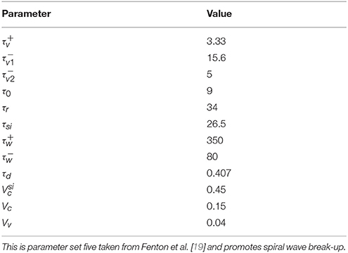
The parameter set shown in Table 1 (taken from [19]) depicts the chosen parameters, which promote spiral wave break-up. During the simulations, snapshots of the membrane potential V_m were taken each 10 time units ($\widehat{=}$ 1 frame).

TABLE 1

Table 1. Parameters used for numerical simulations of the Fenton-Karma model.

2.6.1. 3D Simulation Dataset

For the first dataset which we will refer to as the 3D simulation, Equations (10)–(12) were solved on a regular grid with a grid size of (N_x, N_y, N_z) = (151, 165, 130) (with a grid spacing of h = 0.013cm) using an explicit Euler scheme. A time constant of dt = 0.1 was used, where one time unit may be interpreted as 1 ms for this model and parameter set. The diffusion and grid spacing were chosen to allow a realistic number of filaments to develop. No-flux boundary conditions at the irregular boundary of the realistic heart geometry have been implemented using the phase field method [20, 21]. During the simulations, the sinus rhythm was modeled by local stimuli at the apex of the heart. Episodes of spatio-temporal chaos were then initiated by the application of a far field shock. With the proper timing of this shock, the induced excitation wave creates spiral waves by the interaction with the refractive back of the plane wave which originated from the sinus rhythm. The surface activity was determined by detecting the outer layer of the simulation geometry, and then extracting the excitation patterns from four directions. By this procedure, the surface activity of two opposing directions complement each other to the full surface activity. Thus, neighboring directions cover partially the same excitation activity. In analogy to the experimental setup the different directions are referred to as camera 1–4. A sketch of the setup is shown in Figure 4.

FIGURE 4

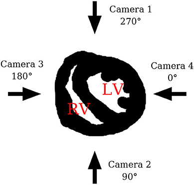
Figure 4. Sketch showing the four different camera perspectives in relation to the heart. LV indicates the position of the left ventricle and RV the position of the right ventricle.

2.6.2. 2D Simulation Dataset

For the second dataset which we will refer to as the 2D simulation, parameters identical to the 3D version were used. The simulation grid was (N_x, N_y) = (400, 400) with the same time step and grid spacing as before. Boundaries were implemented as no-flux boundary conditions and a circular inhomogeneity of radius 60 placed into the center and implemented using the phase field method [20, 21]. A single spiral wave was initiated and simulated for a transient of 5,000 time units before the actual simulation started.

2.6.3. Noise

For the investigation of the effect of noise on the quantities in section 3.3 uniformly distributed random numbers r ∈ [−0.5, 0.5) have been added to V_m as:

$\begin{array}{ll}\begin{array}{l}{V}_{m,a}=V_m+r·a\hfill \end{array}& (17)\end{array}$

We will refer to the two noise amplitudes a = 1 and a = 2 as noise level one and two, respectively. Note that V_m is scaled between zero and one in the model.

The motivation for using this implementation of noise is that we want to investigate the effect of measurement noise which typically arise from optical instruments and camera chips. We explicitly do not want to investigate dynamical noise which would influence the evolution of the model differential equations, as this would lead to different and possibly more complex types of arrhythmia. Furthermore, we do not expect dynamical noise to have a strong influence on the comparison of the methods for quantifying complexity.

3. Results

3.1. Parameter Scan of the Spatial Separation

In this section the effect of varying the spatial separation is investigated using the 3D simulation dataset which was introduced in section 2.6.1. Figure 5 shows snapshots of the 3D simulation.

FIGURE 5

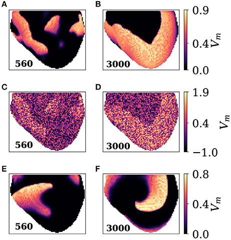
Figure 5. Snapshots of the 3D simulation. (A) Camera 1 at frame 560 showing complex wave activity. (B) Camera 1 at frame 3000 showing plane waves. (C,D) Same as A,B, but with noise added at noise level two. (E,F) Frames 560 and 3000 seen by camera 2. Camera 2 is facing a spiral wave at frame 3000 which causes plane wave activity seen in B.

Figure 6 shows the result of STPE applied to the simulated VF using camera one. In order to show the effect of different values for the spatial separation L_x a spectrogram-like display has been created where the spatial separation is aligned on the y-axis and each row is one time series of nSTPE calculated using this value of L_x. Figures 6B–E show the time series for (non-normalized) STPE for different values of the spatial separation L_x.

FIGURE 6

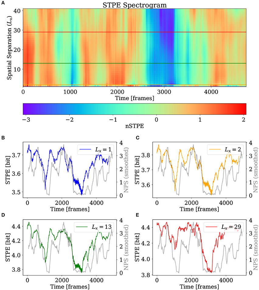
Figure 6. (A) nSTPE displayed for different values of the spatial separation in a spectrogram-like view. (B–E) Show the time series for STPE at different values of the spatial separation together with NPS (gray). The values of L_x are given in the subfigure legends respectively. NPS has been smoothed using a moving average filter with a width of 155 frames.

For comparing the complexity as measured by STPE to a standard measure, NPS has been plotted in gray in Figures 6B–E. NPS can fluctuate heavily, therefore it has been smoothed here using a moving average filter with a width of 155 frames. It can be seen that starting from a spatial separation of L_x = 2 a drop in complexity around frame 2,700 is detected which corresponds to a drop in NPS to zero around the same time. A second very dominant drop in STPE is found around frame 1,000 which is in accordance with NPS which also drops to zero around the same time. In general the match between STPE and NPS seems to be quite good, although some differences are visible especially during the initial period of the simulation and at the end of the video.

The differences for different levels of L_x are not very pronounced for this dataset. However, the possibility to detect complexity at different scales can be a valuable feature of this method. Another example of a STPE spectrogram where differences between the different scales are visible is presented in section 3.4.

3.2. Comparison to SPE and NPS

To compare STPE, SPE, and NPS, the time series of these quantities have been plotted for each camera of the 3D simulation individually in Figure 7. NPS is smoothed with a running average filter with a width of 155 frames. NPS shows that the simulation contains varying complexity in all four camera videos. One special feature is the relatively long period of low complexity starting from approximately frame 2,700. It is visible that camera one (blue) and four (red) record an NPS of zero during this period. The value of NPS as seen from camera three (green) is between zero and one and the value of NPS for camera two (orange) remains approximately one at the same period indicating that one spiral is seen on camera two and partly on camera three while the other cameras register plane waves emerging from that spiral.

FIGURE 7

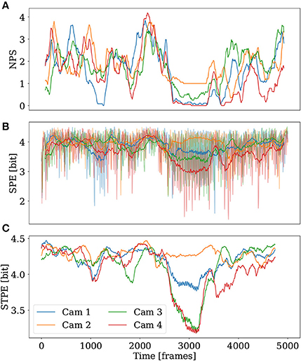
Figure 7. NPS, SPE, and STPE for the four different cameras of the 3D simulation. The spatial separation was fixed to L_x = 14. (A) NPS, smoothed with a running average filter with a width of 155 frames. (B) The raw SPE time series are displayed transparently in (B) in the background. Smoothed time series of SPE are plotted in the foreground. A running average filter with a width of 155 frames has been used. (C) shows the STPE time series.

SPE shows a strongly fluctuating signal which is the reason why for easier interpretation the raw signal has been plotted transparent in the background with a smoothed version of SPE as a thick solid line. The smoothing has been applied using an running mean filter with window length of 155 frames. SPE also registers that during the long low complexity period camera four and partly also camera three and one reveal a low complexity period. At the same time SPE assigns a high complexity for camera two.

STPE shows a very pronounced drop in complexity for camera four and camera three at the long low complexity period, a much less pronounced drop in complexity for camera one and a high complexity in camera two. Similar to SPE also STPE assigns a higher value of complexity to camera one than to camera three which is different to the information extracted from NPS during this period of time. This is a hint that in fact different information than mere information about spiral waves is extracted by the spatial- and spatiotemporal PE.

3.3. Robustness Against Noise

For testing the robustness against noise for SPE and STPE noisy versions of the 3D simulation datasets have been generated as described in section 2.6.3. Figure 8 shows the result of applying NPS, SPE and STPE to the dataset with noise. As a simplification the results are not shown for each camera separately, but the sum of NPS over all cameras and the mean of the permutation entropy quantities are shown. In this case both are displayed, the plain quantities and the normalized quantities which had been introduced in section 2.4.

FIGURE 8

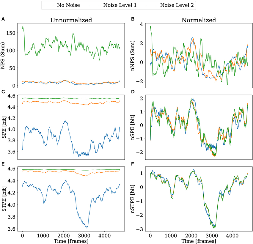
Figure 8. Comparison of NPS, SPE, and STPE under the influence of noise for the case of the 3D simulation dataset. The left column shows the plain quantities without normalization. The right column shows the quantities again with normalization applied. (A,B) The sum of the NPS over all cameras. (C,D) Mean of SPE and nSPE over all cameras. (E,F) Mean of STPE and nSTPE over all cameras. STPE and SPE were computed with L_x = 14 for this comparison.

Our implementation of the NPS detection struggles to find PS in the presence of stronger noise (see also the comments in section 3.5.). While for noise level one (see section 2.6.3 for definitions) it is still possible to identify a period of time around frame 3,000 with less PS, this feature is completely gone for noise level two. As visible in Figure 8A the total number of PS increases strongly. In real applications this problem may be mitigated using smoothing.

SPE and STPE which are displayed in Figures 8C,E generally increase in absolute values. This can be explained by the fact that higher noise leads to a higher variety of order patterns resulting in a flatter distribution for p_j in Equation (3). However, it is still possible to identify all features from the video without noise from the noisy data using the normalized versions of SPE and STPE. Especially in case of nSTPE in Figure 8F all three curves seem to overlap almost perfectly.

3.4. STPE Spectrogram for the 2D Simulation

In order to demonstrate that STPE can be tuned to detect complexities at different scales a parameter scan similar to the one in section 3.1 has been used to generate a STPE spectrogram. This time the method has been applied to the 2D simulation dataset described in section 2.6.2. To illustrate the activity visible in the simulation dataset snapshots are presented in Figure 9. This dataset features many interactions between spiral waves and different levels of complexity. Starting from approximately frame 3,740 only one spiral wave, which is pinned to the circular heterogeneity in the center, remains.

FIGURE 9

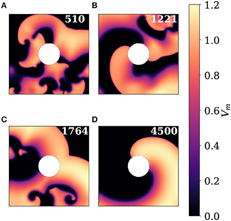
Figure 9. Snapshots showing different regimes of complexity in the 2D simulation dataset. The white circle in the center is a non-conductive heterogeneity. (A) Frame 510 showing lots of interacting spiral waves. (B) Frame 1221 is taken from a regime with two spirals pinned to the heterogeneity and some remaining complex activity in the top right quadrant. (C) In frame 1764 several spiral waves contained mostly in the lower left triangle of the domain generate synchronized plane wave activity that travels to the upper right corner. (D) A single pinned spiral wave remains until the end of the video. This snapshot shows frame 4500.

The STPE spectrogram is visible in Figure 10. This time in addition to the overview of different nSTPE at specific values of L_x in A, and four different excerpts of STPE at some scales, the four snapshots of the simulation which are displayed in Figures 9A–D are marked in Figure 10A as blue vertical lines with the corresponding letter.

FIGURE 10

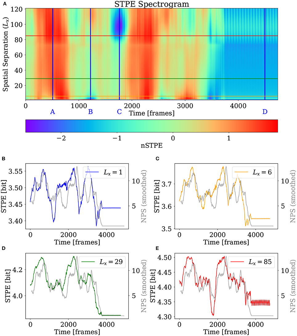
Figure 10. STPE spectrogram and excerpts for the 2D simulation. (A) nSTPE displayed for different values of the spatial separation in a spectrogram-like view. The blue lines annotated with blue letters mark the frames which are shown in Figures 9A–D. (B–E) Show the time series for STPE at different values of the spatial separation together with NPS (gray). NPS has been smoothed using a moving average filter with a width of 155 frames.

It can be seen that the main transition in complexity, the takeover of one pinned spiral at the end of the simulation close to frame 3,700, is clearly visible on all scales. Furthermore it can be seen that the different scales are similar in many features. For example the two periods of high complexity around frames 600 and 2,200 are present in all scales analyzed here. Out of the four excerpts, the one for L_x = 29 seems to match the NPS time series best, but the complexity measured by NPS has a lot of similarity with all excerpts of STPE here.

Two very important differences among the different scales seen here are the drop in complexity at small scales approximately at frame 1,221 marked with the blue B and the big kink for STPE for L_x > 80 around frame 1,764 marked with the blue C. The former feature is not visible in STPE at larger scales while the latter low complexity phase is only reflected in larger scales.

3.5. Speed of Computations

For practical applications speed of computations of the specific methods are highly relevant. The algorithms involved in this article are written in Python using NumPy [22] and SciPy [23]. The implementations of SPE and STPE are written in Cython [24] which generates C code that is afterwards compiled to binary code. The algorithm requires only a single pass over the data and only few basic operations making the compiled code very efficient. The application of the PS analysis involves tracking of PS (see section 2.5.2) which becomes inefficient in the case of a large number of PS. Therefore, this method suffers a lot from noisy data which may in practice be smoothed, but kept here for demonstrational purposes. For comparison, our implementation needs approximately 6 min to identify and track the singularities for the 2D simulation dataset (without noise).

In contrast the speed of computation of SPE and STPE is independent of noise. For the 2D simulation dataset computation of SPE takes approximately 4.3 s and STPE needs less than 5 s. These values have been obtained using an Intel^® Core™ i7-7500U processor at 2.7 GHz (Turbo Boost until 3.5GHz).

4. Discussion

In this article we have presented a detailed analysis of simulated excitable media using SPE and STPE as complexity measures. Because phase singularities can be thought of as the structuring elements of spiral-wave activity on the heart [1] we use it as the baseline for our comparisons.

We find that SPE and STPE can extract complexity information from simulated excitable media which partly corresponds to information extracted by PS analysis.

While the overlap between NPS and the spatial- and spatiotemporal PE is very high in many cases, some differences can be seen which stem from the fact that the PE quantifies the distribution of patterns on the medium and does not favor a specific type of phenomenon such as spiral waves.

We furthermore demonstrated that both, SPE and STPE are very robust under the influence of noise without any computational performance penalty. NPS, in contrast, breaks down for high levels of noise while becoming computationally even more demanding.

It was shown that STPE reveals different levels of complexity at different scales highlighting the possibility to tune it to specific patterns of interest.

In-depth interpretations of the exact levels of complexity at specific scales will require further analysis not covered by this article. However, we conclude that especially STPE provides a very good, fast, and robust alternative for distinguishing high complexity and low complexity periods. The larger speed may especially be relevant in an experiment where time consuming PS analysis is not feasible. Even in a computational context permutation entropy provides a different approach for complexity estimation and comparison with other methods such as Lyapunov dimensions may be interesting, although they are not reliably available for experimental data.

Especially the low susceptibility to noise of SPE and STPE make them suitable for the analysis of massive data from ex-vivo experiments. We plan to apply these methods to recordings of ex-vivo hearts obtained in optical mapping experiments. For these data SPE and STPE can provide a complexity marker additional to phase singularity analysis which will be used for investigating the onset of arrhythmia, the mechanisms of termination and the analysis of complexity variations [25]. We plan to also adapt these methods to other types of signals from cardiac research. In particular the application to ECG signals involving multiple channels, where the low spatial resolution renders phase singularity analysis impossible, might be promising. In addition to the application to multichannel ECG, also investigations of the atrium with basket catheters may allow the transfer of SPE and STPE analysis to clinically relevant settings.

Author Contributions

AS, UP, and SL designed research; AS and SB implemented the algorithms; TL and SB performed simulations; AS analyzed the data; AS, UP, SB, TL, and SL wrote the paper.

Funding

We acknowledge support from the German Federal Ministry of Education and Research (BMBF) (project FKZ 031A147, GO-Bio), the German Research Foundation (DFG) (Collaborative Research Centers SFB 1002 Project C3 and SFB 937 Project A18) and the German Center for Cardiovascular Research (DZHK e.V.). We thank the International Max Planck Research School (IMPRS) Physics of Biological and Complex Systems (PBCS) for financial support.

Conflict of Interest Statement

The authors declare that the research was conducted in the absence of any commercial or financial relationships that could be construed as a potential conflict of interest.

Acknowledgments

We thank Daniel Hornung for providing the CT scan of the rabbit heart which was used for the three-dimensional simulation.

References

1. Winfree AT. Electrical instability in cardiac muscle: phase singularities and rotors. J Theor Biol. (1989) 138:353–405. doi: 10.1016/S0022-5193(89)80200-0

PubMed Abstract | CrossRef Full Text | Google Scholar

2. Gray RA, Pertsov AM, Jalife J. Spatial and temporal organization during cardiac fibrillation. Nature (1998) 392:75–8. doi: 10.1038/32164

PubMed Abstract | CrossRef Full Text | Google Scholar

3. Fenton FH, Luther S, Cherry EM, Otani NF, Krinsky V, Pumir A, et al. Termination of atrial fibrillation using pulsed low-energy far-field stimulation. Circulation (2009) 120:467–76. doi: 10.1161/CIRCULATIONAHA.108.825091

PubMed Abstract | CrossRef Full Text | Google Scholar

4. Pumir A, Sinha S, Sridhar S, Argentina M, Hrning M, Filippi S, et al. Wave-train-induced termination of weakly anchored vortices in excitable media. Phys Rev E (2010) 81:010901. doi: 10.1103/PhysRevE.81.010901

PubMed Abstract | CrossRef Full Text | Google Scholar

5. Luther S, Fenton FH, Kornreich BG, Squires A, Bittihn P, Hornung D, et al. Low-energy control of electrical turbulence in the heart. Nature (2011) 475:235–9. doi: 10.1038/nature10216

PubMed Abstract | CrossRef Full Text | Google Scholar

6. Bandt C, Pompe B. Permutation entropy: a natural complexity measure for time series. Phys Rev Lett. (2002) 88:174102. doi: 10.1103/PhysRevLett.88.174102

PubMed Abstract | CrossRef Full Text | Google Scholar

7. Parlitz U, Berg S, Luther S, Schirdewan A, Kurths J, Wessel N. Classifying cardiac biosignals using ordinal pattern statistics and symbolic dynamics. Comp Bio Med. (2012) 42:319–27. doi: 10.1016/j.compbiomed.2011.03.017

PubMed Abstract | CrossRef Full Text | Google Scholar

8. Ribeiro HV, Zunino L, Lenzi EK, Santoro PA, Mendes RS. Complexity-entropy causality plane as a complexity measure for two-dimensional patterns. PLoS ONE (2012) 7:e40689. doi: 10.1371/journal.pone.0040689

PubMed Abstract | CrossRef Full Text | Google Scholar

9. Schlemmer A, Berg S, Shajahan TK, Luther S, Parlitz U. Quantifying spatiotemporal complexity of cardiac dynamics using ordinal patterns. In: 2015 37th Annual International Conference of the IEEE Engineering in Medicine and Biology Society (EMBC). Milan (2015). p. 4049–4052.

PubMed Abstract | Google Scholar

10. Amigó J. Permutation Complexity in Dynamical Systems. Berlin, Heidelberg: Springer Berlin Heidelberg (2010).

Google Scholar

11. Winfree AT. The Geometry of Biological Time. vol. 12 of Interdisciplinary Applied Mathematics. New York, NY: Springer (2001). doi: 10.1007/978-1-4757-3484-3

CrossRef Full Text | Google Scholar

12. Iyer AN, Gray RA. An experimentalist's approach to accurate localization of phase singularities during reentry. Ann Biomed Eng. (2001) 29:47–59. doi: 10.1114/1.1335538

PubMed Abstract | CrossRef Full Text | Google Scholar

13. Mandapati R, Asano Y, Baxter WT, Gray R, Davidenko J, Jalife J. Quantification of effects of global ischemia on dynamics of ventricular fibrillation in isolated rabbit heart. Circulation (1998) 98:1688–96. doi: 10.1161/01.CIR.98.16.1688

PubMed Abstract | CrossRef Full Text | Google Scholar

14. Lee MH, Qu Z, Fishbein GA, Lamp ST, Chang EH, Ohara T, et al. Patterns of wave break during ventricular fibrillation in isolated swine right ventricle. Am J Physiol Heart Circ Physiol. (2001) 281:H253–65. doi: 10.1152/ajpheart.2001.281.1.H253

PubMed Abstract | CrossRef Full Text | Google Scholar

15. Liu YB, Peter A, Lamp ST, Weiss JN, Chen PS, Lin SF. Spatiotemporal correlation between phase singularities and wavebreaks during ventricular fibrillation. J Cardiovas Electrophysiol. (2003) 14:1103–09. doi: 10.1046/j.1540-8167.2003.03218.x

PubMed Abstract | CrossRef Full Text | Google Scholar

16. Rogers JM. Combined phase singularity and wavefront analysis for optical maps of ventricular fibrillation. IEEE Trans Biomed Eng. (2004) 51:56–65. doi: 10.1109/TBME.2003.820341

PubMed Abstract | CrossRef Full Text | Google Scholar

17. Lorensen WE, Cline HE. Marching cubes: A high resolution 3D surface construction algorithm. In: SIGGRAPH Computer Graphics. Vol. 21, New York, NY: ACM (1987). p. 163–9. doi: 10.1145/37402.37422

CrossRef Full Text | Google Scholar

18. Fenton F, Karma A. Vortex dynamics in three-dimensional continuous myocardium with fiber rotation: Filament instability and fibrillation. Chaos Interdiscipl J Nonlin Sci. (1998) 8:20. doi: 10.1063/1.166311

PubMed Abstract | CrossRef Full Text | Google Scholar

19. Fenton FH, Cherry EM, Hastings HM, Evans SJ. Multiple mechanisms of spiral wave breakup in a model of cardiac electrical activity. Chaos Interdiscipl J Nonlin Sci. (2002) 12:852–92. doi: 10.1063/1.1504242

PubMed Abstract | CrossRef Full Text | Google Scholar

20. Li X, Lowengrub J, Rätz A, Voigt A. Solving PDEs in complex geometries: a diffuse approach. Commun Math Sci. (2009) 7:81–107. doi: 10.4310/CMS.2009.v7.n1.a4

PubMed Abstract | CrossRef Full Text | Google Scholar

21. Fenton FH, Cherry EM, Karma A, Rappel WJ. Modeling wave propagation in realistic heart geometries using the phase-field method. Chaos Interdiscipl J Nonlin Sci. (2005) 15:013502. doi: 10.1063/1.1840311

PubMed Abstract | CrossRef Full Text | Google Scholar

22. van der Walt S, Colbert SC, Varoquaux G. The NumPy array: a structure for efficient numerical computation. Comput Sci. Eng. (2011) 13:22–30. doi: 10.1109/MCSE.2011.37

CrossRef Full Text | Google Scholar

23. Jones E, Oliphant T, Peterson P, et al. SciPy: Open source scientific tools for Python. (2001). Online; accessed 2018-01-15. Available online at: http://www.scipy.org/

Google Scholar

24. Behnel S, Bradshaw R, Citro C, Dalcin L, Seljebotn DS, Smith K. Cython: the best of both worlds. Comput Sci. Eng. (2011) 13:31–9. doi: 10.1109/MCSE.2010.118

CrossRef Full Text | Google Scholar

25. Schlemmer A, Baig T, Luther S, Parlitz U. Detection and characterization of intermittent complexity variations in cardiac arrhythmia. Physiol Measure. (2017) 38:1561. doi: 10.1088/1361-6579/aa7be0

PubMed Abstract | CrossRef Full Text | Google Scholar