- 1College of Information Science and Engineering, Northeastern University, Shenyang, China
- 2Department of Neurology, Cincinnati Children's Hospital Medical Center, Cincinnati, OH, United States
Background: Convolution neural networks (CNN) is increasingly used in computer science and finds more and more applications in different fields. However, analyzing brain network with CNN is not trivial, due to the non-Euclidean characteristics of brain network built by graph theory.
Method: To address this problem, we used a famous algorithm “word2vec” from the field of natural language processing (NLP), to represent the vertexes of graph in the node embedding space, and transform the brain network into images, which can bridge the gap between brain network and CNN. Using this model, we analyze and classify the brain network from Magnetoencephalography (MEG) data into two categories: normal controls and patients with migraine.
Results: In the experiments, we applied our method on the clinical MEG dataset, and got the mean classification accuracy rate 81.25%.
Conclusions: These results indicate that our method can feasibly analyze and classify the brain network, and all the abundant resources of CNN can be used on the analysis of brain network.
Introduction
Brain network and brain functional/structural connectivity play an important role in neuroanatomy, neurodevelopment, electrophysiology, functional brain imaging, and neural basis of cognition (Hosseini et al., 2012). Recently, more and more graph theoretical analyses have been used to quantitatively measure the brain network of neuroimaging data. Niso et al. (2015) recorded magnetoencephalographic (MEG) data from 45 subjects (15 healthy controls and 30 migraine patients) during interracial testing state with closed eyes, and calculated 15 graph-theoretic measures to compare brain network characterizations between healthy controls and epileptic patients. Their results showed that differences in spectral power between the control and the epileptic groups have a distinctive pattern, which indicate that functional epileptic brain networks are different to those of healthy subjects during interictal stage at rest. Bassett and Bullmore (2006, 2017) analyzed the brain network using graph theoretical measures, which were clustering coefficient and path length, and concluded that the brain network had a small-world topology characterized by a high clustering coefficient between neighboring nodes and a short path length between any pair of nodes. Sherman et al. (2014) studied development of the default mode network across early adolescence based on graph theory, and found that brain network measures, such as integration, segregation, and connectivity, increased as the participants' age grow.
According to graph theory, brain networks can be composed of nodes and edges. The nodes represent neurons or brain regions, and the edges represent the physical or functional connections between nodes. Therefore, the brain network analysis using graph theory can be composed of four steps (Bullmore and Sporns, 2009): (1) define the network nodes, (2) define the measure of connections between nodes, (3) generate a adjacent matrix or undirected graph by calculating the pairwise associations between nodes, (4) calculate the graph theoretical parameters which can locally or globally characterize the brain network. Although, graph theory is widely used to analyze the brain network, there are still some shortcomings in the framework. Until now, many mathematical definitions of brain network measures have been presented, such as degree, shortest path length (Watts and Strogatz, 1998), number of triangles, global/local efficiency (Latora and Marchiori, 2001), clustering coefficient (Watts and Strogatz, 1998), transitivity (Newman, 2003), modularity (Newman, 2004), closeness centrality (Freeman, 1978), betweenness centrality (Freeman, 1978), within-module degree z-score (Guimerà and Amaral, 2005), participation coefficient (Guimerà and Amaral, 2005), anatomical and functional motifs (Milo et al., 2002; Sporns and Kotter, 2004), motif z-score(Milo et al., 2002), motif fingerprint (Sporns and Kotter, 2004), degree distribution (Barabasi and Albert, 1999), average neighbor degree (Pastor-Satorras et al., 2001), assortativity coefficient (Newman, 2002), measure of small-worldness (Humphries and Gurney, 2008). All these measures have different specific advantage and suitable for different fields, respectively, for example, shortest path length and global efficiency are suitable for measuring integration of brain network, clustering coefficient, local efficiency, and transitivity are suitable for measuring segregation of brain network, centrality and within-module degree z-score are suitable for measuring the centrality of brain network, motif z-score and motif fingerprint are suitable to measuring the brain network motifs, degree distribution, average neighbor degree, and assortativity coefficient are suitable for measuring the resilience of brain network. Therefore, different measures have different emphasis and performance on analyzing the brain network, which even result into totally conflicting results. Two studies (Leistedt et al., 2009; Zhang et al., 2011) found that major depressive disorder (MDD) patients had lower shortest path length compared with normal controls, and no significant differences in clustering coefficient. However, another study (Lord et al., 2012) found that MDD patients had a significant change of the community structures compared with healthy controls, but there was no significant differences in shortest path length and clustering coefficient.
In the last few years, convolutional neural network (CNN) has performed very well in many fields, such as image processing, artificial intelligence, human speech recognition, computer-aided diagnosis, natural language processing (NLP), and so on. The development of CNN can be tracked back in 1968, which is interestingly motivated by neuroscience findings. In 1968, Hubel and Wiesel (1968) found that cells in animal visual cortex are responsible for detecting light in receptive fields. Inspired by their findings, Kunihiko Fukushima proposed the neocognitron in 1980 (Fukushima and Miyake, 1982). Next, in 1990, LeCun et al. (1989) improved neocognitron and proposed LeNet-5 (LeCun et al., 1998), which can be recognized as the predecessor of CNN. LeNet-5 was composed of many artificial neural network layers and can be trained with backpropagation method. However, due to the poor performance of the computers at the time, the training of CNN is desperately time consuming, which means that CNN cannot resolve complicated problems at that time. As the rapid and huge development of computer hardware and software framework, as well as the Big Data technology, CNN comes back into researchers' vision again. In 2012, Krizhevsky et al. improved traditional CNN and proposed AlexNet (Krizhevsky et al., 2012), which is similar to LeNet-5 but with a deeper structure. After that, ZFnet (Zeiler and Fergus, 2014), VGGNet (Simonyan and Zisserman, 2015), GoogleNet (Szegedy et al., 2015), ResNet (He et al., 2016), etc., were proposed, all these CNN structures became deeper and deeper, and can resolve many complicated problems in image, video, and speech processing tasks. However, image, video, and speech data are represented by 1D or 2D Euclidean space discretized by rectangles, which means that CNN are suitable for these kinds of regular, grid-like, low-dimensional data. Besides Euclidean space data (image, video, speech), there are also irregular or non-Euclidean domains that can be structured with graphs, such as user data on social networks, gene data on biological regulatory networks, log data on telecommunication networks, text documents on word embeddings (Defferrard et al., 2016), as well as brain networks which is our concern in this paper.
Although, CNN has got outstanding performance in Euclidean space data, generalization of CNN to irregular or non-Euclidean data ( represented by graph) is not trivial, because the operators in CNN (convolution, pooling, Relu, dropout, etc. ) are only defined for regular grids. Analyzing the graph based on CNN is a new topic, Defferrard et al. (2016) and Kipf and Welling (2017) invoke the convolution theorem from signal processing theory and transform the graph to Fourier domain by SVD decomposition of the graph Laplacian matrix, whose eigenvalues are recognized as “frequencies” (Tixier et al., 2017). By contrast, Niepert et al. (2016) don't operate the CNN graph in the Fourier domain, they imitate the image-based convolution networks and present a general approach to extracting locally connected regions from graphs. Kawahara et al. (2017) propose novel convolution filters that leverage the topological locality of structural brain networks, in contrast to the spatially local convolutions done in the traditional image-based CNN. And they use this framework to predict clinical neurodevelopmental outcomes from brain networks.
In the present study, we aim to classified the brain network into normal group and migraine group using the MEG data from normal controls and patients with migraine. We construct the brain network using graph theory, then analyze the brain network based on CNN, instead of carefully and elaborately choosing one or several graph measures to quantitatively delineate the brain network and result in a significant difference or mathematical relationship, which may be conflicting if another measures are picked. The main contributions of the present study are: (1) build a bridge between brain network and CNN, so that the abundant CNN toolkits and methods can be used to analyze brain network; (2) the first study that classify the brain network into two categories, which are normal and abnormal (migraine); (3) represent the graph as an image and classify the graph by extracting features by building a CNN structure from the images.
Methods
The main steps of our method are: (1) construct a brain network using graph theory; (2) represent the graph as an image; (3) build a CNN structure; (4) analyze and classify the transformed images based on CNN. And the schematic of our method is show in Figure 1.
Building Brain Network
Before building brain network, there are some preprocessing on the raw MEG data. Noticeable noise or artifacts were excluded using FieldTrip (an open source MATLAB toolbox, http://www.fieldtriptoolbox.org/start), and the preprocessing steps are: (1) Define segments of interest; (2) Read the MEG data (with padding) from disk; (3) Filter the data; (4) Z-transforme the filtered data and averaging it over channels; (5) Threshold the accumulated z-score.
Mathematically, brain network is represented by ordered pairs of set G(N, L) in which N is a set of nodes and L is a set of links. Graphically, the nodes are plotted as points and the links as lines joining them. When two nodes are connected by a link, they are considered neighbors (or adjacent) (Wang and Meng, 2016). In the present study, we used 275 MEG sensors as the graph nodes, and used phase lag index (PLI) (Luis et al., 2016) as the functional connections between nodes, which are graph edges.
Δj represents the phase difference between two time series, k represents the time-point, sign represents signum function, < > represents the mean value and | | represents the absolute value. The schematic of building brain network is shown is Figure 2.
Represent a Graph as an Image
This is the core contents of this study. Suppose that we have a graph G(V, E) after building the brain network, V represents the nodes of the graph and the element vi represents the ith node, E represents the edges of the graph and the element ei, j represents the weight between node vi and vj. So the adjacency matrix A can be obtained, which is a square and symmetric matrix with the dimensionality of |V| × |V|, and the element ai, j equals to ei, j. However, graph adjacency matrix does not have spatial dependence property. Therefore, we cannot directly input the graph adjacency matrix to the 2D CNN. To resolve this problem, we represent a graph as an image based on graph node embedding.
Graph Node Embedding
Given a graph G(V, E), a graph embedding is defined as a mapping f :
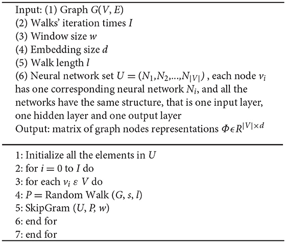
Therefore, the graph embedding space maps each node in the graph to a low dimensional vector, and the proximity between two nodes can be represented as the Euclidean distance between two vectors in the graph embedding space. In the present study, we calculate the mapping function f from graph to node embedding space, which was inspired by a NLP method, that is “Word2Vec” (Mikolov et al., 2013). Using Word2Vec method, all the words in the corpus can be represented as a low dimensional vector, instead of a high dimensional one-hot vector, and the reduction of vector dimensionality can extremely enhance the performance of many NLP tasks, such as word storage, semantic analysis, language translation, and so on. And in our study, we denoted random walk as a stochastic process which was rooted at a node k0 in the brain network and randomly chose another nodes k1,k2,…ki in the neighbor of node k0. Random walk can characterize the neighboring structure of the rooted node in the brain network. Therefore, we can use a serial of random walks to illustrate the information of brain network structure, that is to say, the relationship between brain network nodes and edges. Motivated by the Word2Vec in NLP, we assume that the random walks in a brain network can be thought as sentences and phrases in a language, and all the nodes in the random walks can be though as words in a language, so we can learn not only a probability distribution of node co-occurrences, but also a representation of nodes in the format of vectors. Similarly, we name our method “Node2Vec.” The algorithm pseudo-code of Node2Vec is shown in Algorithm 1.
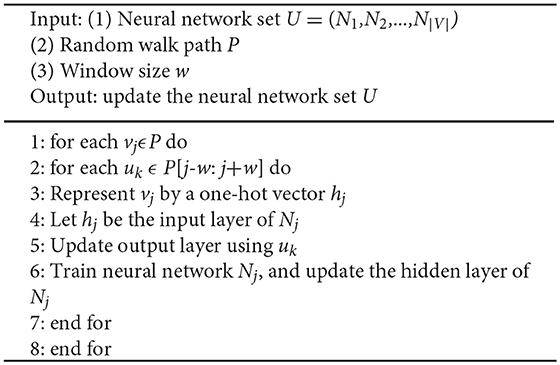
Each node vi in the graph has one corresponding neural network Ni. The input layer of Ni is a 1 × |V| one-hot vector, there is only one “1” in the one-hot vector and the index of “1” indicates the specific node vi. The output layer of Ni is a 1 × |V| vector, and each item of vector indicates the possibility that the corresponding node is in the neighbor of node Ni. The hidden layer of Ni is a 1 × d vector ( d < < |V| ), this is the mapping function f we're looking for, it means that the corresponding node in the input layer can be represented by the vector in the hidden layer, which is represented in formula (1).
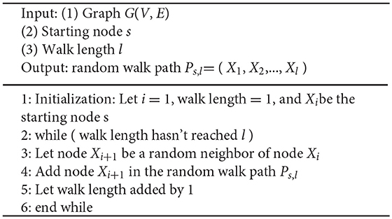
Line 4 and 5 are the core steps of Node2Vec algorithm. Given a graph G(V, E), we denote random walk of length l rooted from node s as a stochastic process with random variables X1, X2,…, Xl, such that X1 = s and Xi+1 is a vertex chosen randomly from the neighbors of Xi. We used random walk to extract local structure information from the network. The algorithm pseudo-code of random walk is shown in Algorithm 2. SkipGram algorithm maximizes the co-occurrence probability among the nodes in a window (Mikolov et al., 2013), and the algorithm pseudo-code is shown in Algorithm 3.
Represent Graph as Image
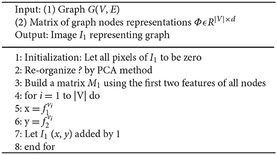
In the graph node embedding space, we obtain the matrix of graph nodes representations ΦϵR|V| × d, so we can represent each node vi in the graph as a d-dimension vector. And in the viewpoint of machine learning, we can also conclude that each node vi in the graph has d features. Next, we need to align all these features to determine which feature is the most important one, which dimensional is the second important one, and so on. Therefore, in this paper, principle component analysis (PCA) method is used to transform the d-dimension vector of node vi into dPCA-dimension vector LPCA, which is a sequential list.
|V| represents the number of nodes in the graph. Then, we can build a matrix M1 using the first two features of all nodes,
represents the first feature of node vi, represents the second feature of node vi. Then we normalize and to a fixed number r of equally-size bins. Then we can build the image I1, the resolution of the image I1 is r × r, and the value of image pixels are defined as the count of the number of nodes falling into that bin. The algorithm pseudo-code is shown in Algorithm 4.
Similarly, we also can build image I2 using the third and fourth features of all nodes, build image I3 using the fifth and sixth features of all nodes, and so on. Totally, we can build dPCA/2 images from the graph node embedding space. However, we don't have to use all the dPCA /2 images, because PCA method is used to reduce and align the features into a sequential list. In this study, we only use the first four features to build two images I1 and I2, which is enough to analyze and classify the brain network, shown in Figure 3.
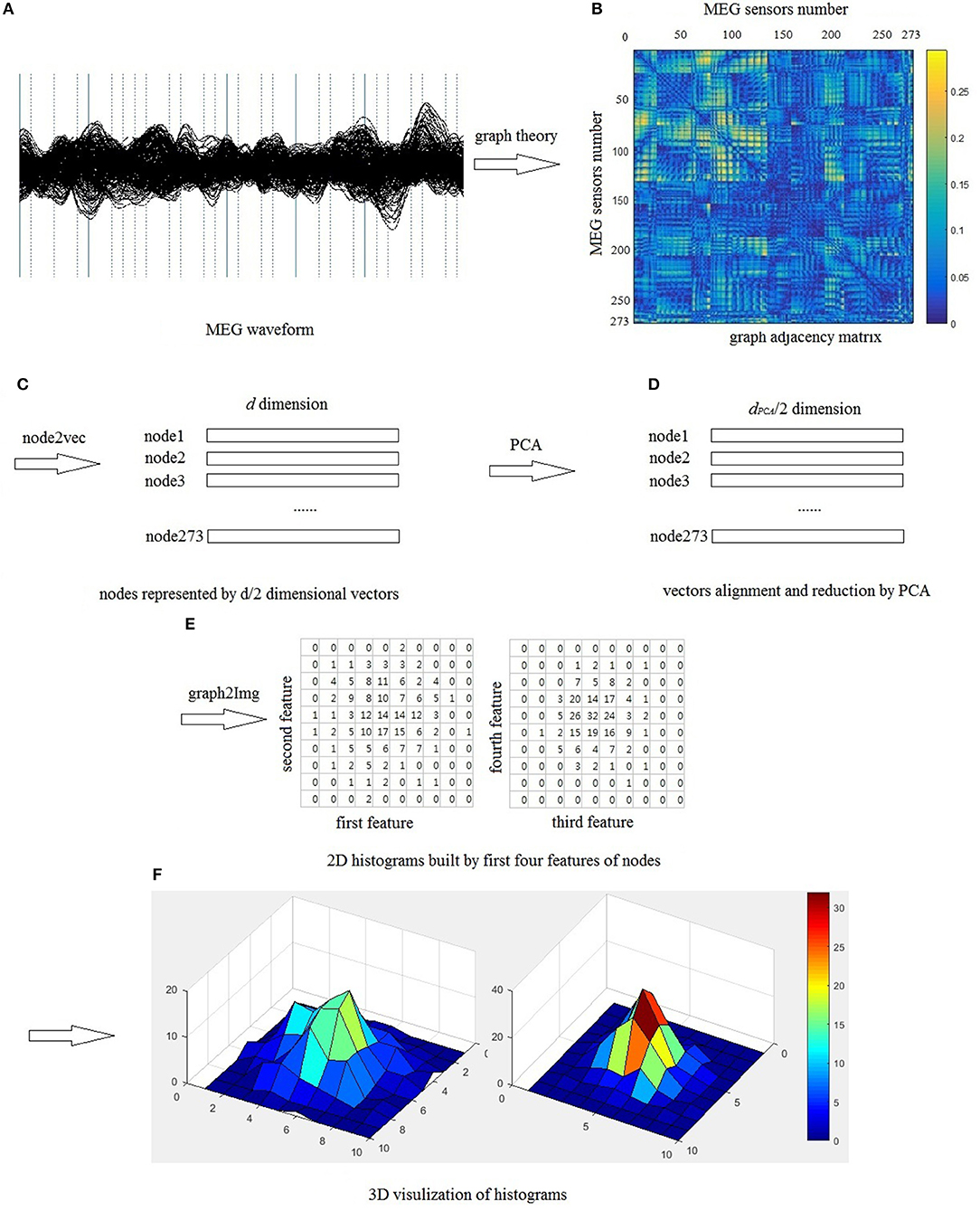
Figure 3. Schematic of representing graph as images, (A) segments of MEG waveform from a healthy control, (B) use 273 sensors as nodes, PLI as edges to build brain network, (C) each in the graph is represented by a d/2 dimensional vector, (D) use PCA method to align and reduce the vectors, (E) build 2D histogram, in this study, each feature is divided into ten bins, therefore, each value in the 10 × 10 matrix is the number of nodes falling into the corresponding bin, and the sum of all pixel values is 273, which is the number of sensors, (F) 3D visualization of histogram.
CNN Architecture
The brain network is represented by two images I1 and I2. We can also recognize I1 and I2 as two channels of one image, just like (R,G,B) channels in the color images. Then we can use these images as an input to CNN. In this study, our CNN structure is based on LeNet-5 (LeCun et al., 1998), there are seven layers totally, including input layer (I1), convolution layer 1 (C2), convolution layer 2 (C3), pooling layer (P4), full connection layer 1 (F5), full connection layer 2 (F6), and output layer (F7), shown as Figure 4.
Firstly, the input layer is a 10 × 10 image. Then, the first convolution layer is 32 kernels of 3 × 3 feature map, each kernel computes a convolution of the input image with a ReLU activation function. The second convolution layer is 128 kernels of 3 × 3 feature map with a ReLU activation function, followed by a 2 × 2 max pooling layer. Next, there two fully-connected layers with 32 nodes and 16 nodes. Finally, the output layer with two output nodes is used to classify the input images into two categories based on the softmax function.
Experiment and Result
In this section, we applied our method on the clinical MEG dataset, which is consists of 40 subjects, 20 healthy controls (subject ID: 1 to 20) and 20 patients with migraine (subject ID: 21–40). All these MEG data were obtained from Cincinnati Children's Hospital Medical Center (CCHMC) and Nanjing Brain Hospital, and the target is to classify MEG data into two classes: the abnormal subjects and the healthy controls.
Our method use some open-source toolkits, MEG data is pre-processed by using FieldTrip toolkit (Oostenveld et al., 2011), brain network is built by using FieldTrip toolkit, graph node embedding is calculated by using node2vec toolkit (Grover and Leskovec, 2016), PCA is performed by using Matlab PCA toolkit, histogram of vectors is calculated by using histograms python toolkit (Tixier et al., 2017), our CNN is implemented using the Keras model with tensorflow (Abadi et al., 2016) backend. All these algorithms are run on Intel Core i7-6700 3.4 GHz CPU and 8 GB of RAM, under Windows 7 × 64 operating system and Python 3.5.
In this study, brain networks of MEG data are represented as images with two channels and resolution 10 × 10. We perform 4-fold cross-validation; the 40 MEG datasets are randomly split into four equal size subsamples. In each run, three subsamples are selected as the train grouping, and the remaining single subsample is retained as the test group. Input all these images of train group into our CNN architecture, and the categorical cross-entropy loss is optimized with Adam. To avoid over-fitting, dropout = 0.25 is used after convolution layers C2, C3 and fully-connected layer F5, and early stopping is also used after every epoch, so the number of epochs of each run is different. The training parameters are as following: dropout rate = 0.25, regularization weight = 5 × 10⁻⁴, learning rate = 0.001, momentum = 0.1, training epoch = 1,000, iteration = 10. After training from CNN, the filter kernels of convolution layers (C2, C3) and the weights of full-connected layers (F5, F6) can be determined, then the training results can be used to validate the test group.
The schematics of the whole procedure of one healthy control (subject ID = 10) and one patient with migraine (subject ID = 30) were shown in Figures 5, 7. And we can see that it's not clear to distinguish the differences between healthy controls and patients with migraine in the brain network (Figure 5) or in the node embedding space (Figure 6), however, in the representation of two-channel images (Figure 7), the differences can be easily found and classified by CNN.
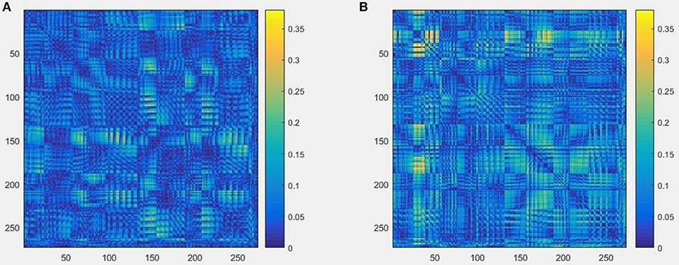
Figure 5. An example of brain network result built from raw MEG data, and the size is 273 × 273, (A) one healthy control (subject ID = 10), (B) one patient with migraine (subject ID = 30).

Figure 6. An example of node2vec result built from brain network, each node of the brain network was represented as a 20-dimensional vector in the node embedding space, so the size was 273 × 20, (A) one healthy control (subject ID = 10), (B) one patient with migraine (subject ID = 30).
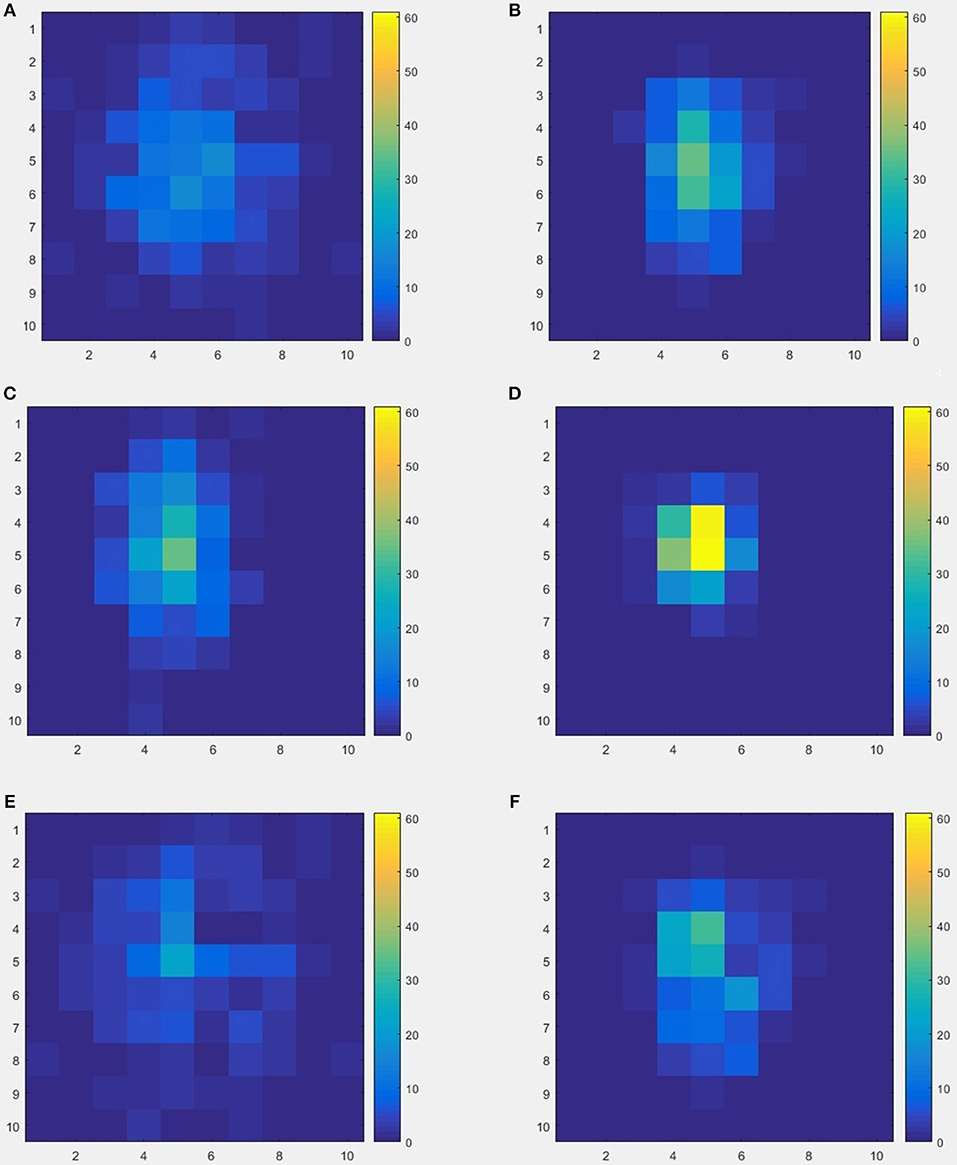
Figure 7. An example of two-channel images results by from 20-dimensional node vectors, each subject was represented as an image with two channels, so the image size is 10 × 10 × 2, (A,B) represent the two channels from one healthy control (subject ID = 10), (C,D) represent the two channels from one patient with migraine (subject ID = 30), (E,F) represent the differences between healthy control and patient.
In this experiment, we repeat the training and testing procedures ten iterations to ensure the stability of the method. Limited by the article length, we can't show all the results from 10 iterations. Therefore, from the iteration #1 of 4-fold cross-validation, we illustrate the validation accuracy rate of every 25 epochs and validation loss rate of every 25 epochs, which are shown in Figures 8–11. The accuracy rate and loss rate were steady after 300 epochs. The classification accuracy rate of four cross-validation are shown in Table 1. Therefore, we may conclude that our method can analyze and classify the brain network into two categories: normal and migraine. After training of 10 iterations, we can obtain the model and weights of each layer. Visualization of weights in all layers from our CNN is shown in Figure 12. Figure 12A shows the weights of the first convolve layer with size (3, 3, 2, 32); Figure 12B shows the weights of the second convolve layer with size (3, 3, 32, 128); Figure 12C shows the weights of the first fully-connected layer with size (1152, 32); Figure 12D shows the weights of the second fully-connected layer with size (32, 16); Figure 12E shows the weights of the third fully-connected layer with size (16, 2). By the visualization, we can see that our convolution kernel size is only 3 × 3, we didn't choose the bigger one, because the resolution of our target is 10 × 10, and large kernel may hinder feature extraction by the feature maps. However, as a remedy for the small kernel size, we used large amount of feature maps and units in the convolve layers and fully-connected layers, and the total number of parameters in our CNN is 74,784, which can make sure that the differences between healthy controls and patients with migraine can be extracted by our CNN.

Figure 8. Testing results of the first run, each dot in the image represents the mean value of every 25 epochs, (A) mean accurate rate of test group, (B) mean loss rate of the group.

Figure 9. Testing results of the second run, each dot in the image represents the mean value of every 25 epochs, (A) mean accurate rate of test group, (B) mean loss rate of the group.

Figure 10. Testing results of the third run, each dot in the image represents the mean value of every 25 epochs, (A) mean accurate rate of test group, (B) mean loss rate of the group.

Figure 11. Testing results of the fourth run, each dot in the image represents the mean value of every 25 epochs, (A) mean accurate rate of test group, (B) mean loss rate of the group.
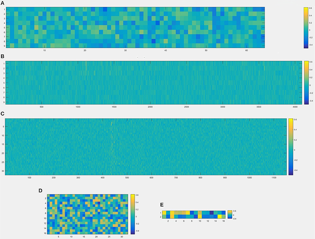
Figure 12. Visualization of weights in all layers from convolutional neural network, (A) the first convolve layer with size (3, 3, 2, 32), which means that there are 64 kernels whose size are 3 × 3, and this layer is visualized by a 9 × 64 image; (B) the second convolve layer with size (3, 3, 32, 128), which means that there are 4,096 kernels whose size are 3 × 3, and this layer is visualized by a 9 × 4096 image; (C) the first fully-connected layer with size (1152, 32), which means that 1,152 units from the output of the last layer and 32 units from the input of first fully-connected layer, and this layer is visualized by a 1,152 × 32 image; (D) the second fully-connected layer with size (32, 16), which means that 32 units from the output of the last layer and 16 units from the second fully-connected layer, and this layer is visualized by a 32 × 16 image; (E) the third fully-connected layer with size (16, 2), which means that 16 units from the last layer and 2 classifications as the output result (normal or migraine), and this layer is visualized by a 16 × 2 image.
Besides, we also compared our classification results with the other two base line methods, Linear SVM and graph convolution neural network (GCNN) from Defferrard et al. (2016), shown in Table 2. Linear SVM is a classical supervised learning method for classification and regression analysis, but for the classification of MEG raw data, the mean accuracy rate is only 58.37%, we guess the poor performance is due to the huge amount of MEG channels, and multiple dimensionalities of MEG data. GCNN and our method both outperform Linear SVM, which indicates that the integration of graph theory and CNN can greatly enhance the performance of classification accuracy, however, GCNN has not made special optimization for MEG data, so it lags behind our method in classification accuracy.
Conclusion and Future Work
In this paper, we bridge the gap between brain network and convolution neural network, and classify the brain network from MEG data into two categories: normal and migraine. We train the CNN architecture on the training group, and validate the result on the testing group, which indicates that our method is feasible and can distinguish normal and migraine brain network.
Next, we will mainly focus on two aspects: (1) collect more MEG data, and improve the CNN architecture; (2) diversify the abnormal MEG brain network, and use our method on the epileptic brain network, autism brain network, and so on; (3) analyze the brain network at the source level.
Author Contributions
LM corresponding author, main contributor. JX data provider and professional advisor.
Conflict of Interest Statement
The authors declare that the research was conducted in the absence of any commercial or financial relationships that could be construed as a potential conflict of interest.
Acknowledgments
This study was partially supported by a Trustee Grant from Cincinnati Children's Hospital Medical Center and Grant Numbers 1R21NS081420 and R21NS072817 from the National Institute of Neurological Disorders and Stroke (NINDS), the National Institutes of Health. We thank Mr. Nat Hemasilpin, Ms.Hisako Fujiwara and Dr. Douglas Rose for assistance and technical support during MEG recordings and Mr. Kendall O'Brien for his technical help in performing MRI scans. This paper was also supported by National Natural Science Foundation of China (No.61101057) and the Fundamental Research Funds for the Central Universities (No. N130404027).
References
Abadi, M., Barham, P., Chen, J., Davis, A., Dean, J., Devin, M., et al. (2016). “TensorFlow: a system for large-scale machine learning.” in Proceedings of the 12th USENIX conference on Operating Systems Design and Implementation (Savannah, GA), 265–283.
Barabasi, A. L., and Albert, R. (1999). Emergence of scaling in random networks. Science 286, 509–512. doi: 10.1126/science.286.5439.509
Bassett, D. S., and Bullmore, E. D. (2006). Small-world brain networks. Neuroscientist 12, 512–523. doi: 10.1177/1073858406293182
Bassett, D. S., and Bullmore, E. T. (2017). Small-world brain networks revisited. Neuroscientist 23, 499–516. doi: 10.1177/1073858416667720
Bullmore, E., and Sporns, O. (2009). Complex brain networks: graph theoretical analysis of structural and functional systems. Nat. Rev. Neurosci. 10, 186–198. doi: 10.1038/nrn2575
Defferrard, M., Bresson, X., and Vandergheynst, P. (2016). “Convolutional neural networks on graphs with fast localized spectral filtering,” in 30th Conference on Neural Information Processing Systems (Barcelona).
Freeman, L. C. (1978). Centrality in social networks: conceptual clarification. Soc. Netw. 1, 215–239.
Fukushima, K., and Miyake, S. (1982). Neocognitron: a self-organizing neural network model for a mechanism of visual pattern recognition. Compet. Cooperat. Neural Net. 45, 267–285. doi: 10.1007/978-3-642-46466-9_18
Grover, A., and Leskovec, J. (2016). node2vec: scalable feature learning for networks. KDD 2016, 855–864. doi: 10.1145/2939672.2939754
Guimerà, R., and Amaral, L. A. (2005). Cartography of complex networks: modules and universal roles. J. Stat. Mech. 2005:P02001. doi: 10.1088/1742-5468/2005/02/P02001
He, K., Zhang, X., Ren, S., and Sun, J. (2016). “Deep residual learning for image recognition,” in Proceedings of the IEEE Conference on Computer Vision and Pattern Recognition (CVPR) (Las Vegas, NV), 770–778.
Hosseini, S. M., Hoeft, F., and Kesler, S. R. (2012). GAT: A graph-theoretical analysis toolbox for analyzing between-group differences in large-scale structural and functional brain networks. PLoS ONE 7:e40709. doi: 10.1371/journal.pone.0040709
Hubel, D. H., and Wiesel, T. N. (1968). Receptive fields and functional architecture of monkey striate cortex. J. Physiol. 195, 215–243. doi: 10.1113/jphysiol.1968.sp008455
Humphries, M. D., and Gurney, K. (2008). Network ‘small-world-ness’: a quantitative method for determining canonical network equivalence. PLoS ONE 3:e0002051. doi: 10.1371/journal.pone.0002051
Kawahara, J., Brown, C. J., Miller, S. P., Booth, B. G., Chau, V., Grunau, R. E., et al. (2017). BrainNetCNN: convolutional neural networks for brain networks; towards predicting neurodevelopment. NeuroImage. 146, 1038–1049. doi: 10.1016/j.neuroimage.2016.09.046
Kipf, T. N., and Welling, M. (2017). “Semi-supervised classification with graph convolutional networks,” in 5th International Conference on Learning Representations (Toulon).
Krizhevsky, A., Sutskever, I., and Hinton, G. E. (2012). “ImageNet classification with deep convolutional neural networks,” in Proceedings of the 25th International Conference on Neural Information Processing Systems, Vol. 25, (Lake Tahoe, NV), 1097–1105.
Latora, V., and Marchiori, M. (2001). Efficient behavior of small-world networks. Phys. Rev. Lett. 87:198701. doi: 10.1103/PhysRevLett.87.198701
LeCun, B. B., Denker, J. S., Henderson, D., Howard, R. E., Hubbard, W., Jackel, L. D., et al. (1989). “Handwritten digit recognition with a back-propagation network,” in Proceedings of the Advances in Neural Information Processing Systems (NIPS) (Denver, CO), 396–404.
LeCun, Y., Bottou, L., Bengio, Y., and Haffner, P. (1998). Gradient-based learning applied to document recognition. Proc. IEEE. 86, 2278–2324. doi: 10.1109/5.726791
Leistedt, S. J., Coumans, N., Dumont, M., Lanquart, J. P., Stam, C. J., and Linkowski, P. (2009). Altered sleep brain functional connectivity in acutely depressed patients. Hum. Brain Mapp. 30, 2207–2219. doi: 10.1002/hbm.20662
Lord, A., Horn, D., Breakspear, M., and Walter, M. (2012). Changes in community structure of resting state functional connectivity in unipolar depression. PLoS ONE 7:e41282. doi: 10.1371/journal.pone.0041282
Luis, R. P., Aziz, U. R. A., Gary, G., and David, M. H. (2016). Volume conduction effects in brain network inference from electroencephalographic recordings using phase lag index. J. Neurosci. Methods. 207, 189–199. doi: 10.1016/j.jneumeth.2012.04.007
Mikolov, T., Chen, K., Corrado, G., and Dean, J (2013), “Efficient estimation of word representations in vector space,” in International Conference on Learning Representation (Scottsdale, AZ), 1–12.
Milo, R., Shen-Orr, S., Itzkovitz, S., Kashtan, N., Chklovskii, D., and Alon, U. (2002). Network motifs: simple building blocks of complex networks. Science 298, 824–827. doi: 10.1126/science.298.5594.824
Newman, M. E. J. (2002). Assortative mixing in networks. Phys. Rev. Lett. 89:2087011–2087014. 10.1103/PhysRevLett.89.208701
Newman, M. E. J. (2003). The structure and function of complex networks. SIAM Rev. 45:167–256. doi: 10.1137/S003614450342480
Newman, M. E. J. (2004). Fast algorithm for detecting community structure in networks. Phys. Rev. E69:066133. doi: 10.1103/PhysRevE.69.066133
Niepert, M., Ahmed, M., and Kutzkov, K. (2016). “Learning convolutional neural networks for graphs,” in Proceedings of the 33rd Annual International Conference on Machine Learning (New York, NY).
Niso, G., Carrasco, S., Gudín, M., Maestú, F., del-Pozo, F., and Pereda, E. (2015). What graph theory actually tells us about resting state interictal MEG epileptic activity. NeuroImage Clin. 8, 503–515. doi: 10.1016/j.nicl.2015.05.008
Oostenveld, R., Fries, P., Maris, E., and Schoffelen, J. M. (2011). FieldTrip: open source software for advanced analysis of meg, eeg, and invasive electrophysiological data. Computat. Intell. Neurosci. 2011:156869. doi: 10.1155/2011/156869
Pastor-Satorras, R., Vázquez, A., and Vespignani, A. (2001). Dynamical and correlation properties of the internet. Phys. Rev. Lett. 87:258701. doi: 10.1103/PhysRevLett.87.258701
Sherman, L. E., Rudie, J. D., Pfeifer, J. H., Masten, C. L., McNealy, K., and Dapretto, M. (2014). Development of the default mode and central executive networks across early adolescence: a longitudinal study. Dev. Cogn. Neurosci. 10, 148–159. doi: 10.1016/j.dcn.2014.08.002
Simonyan, K., and Zisserman, A. (2015). “Very deep convolutional networks for large-scale image recognition,” in Proceedings of the International Conference on Learning Representations (ICLR) (San Diego, CA).
Sporns, O., and Kotter, R. (2004). Motifs in brain networks. PLoS Biol. 2, e369. doi: 10.1371/journal.pbio.0020369
Szegedy, C., Liu, W., Jia, Y., Sermanet, P., Reed, S., Anguelov, D., et al. (2015). “Going deeper with convolutions,” in Proceedings of the IEEE Conference on Computer Vision and Pattern Recognition (CVPR) (Boston, MA), 1–9.
Tixier, A. J. P., Nikolentzos, G., Meladianos, P., and Vazirgiannis, M. (2017). Classifying Graphs as Images with Convolutional Neural Networks. Avaialble online at: https://arxivorg/abs/170802218
Wang, B., and Meng, L. (2016). Functional brain network alterations in epilepsy: a magnetoencephalography study. Epilepsy Res. 126, 62–69. doi: 10.1016/j.eplepsyres.2016.06.014
Watts, D. J., and Strogatz, S. H (1998), Collective dynamics of ‘small-world’ networks Nature 393, 440–442.
Zeiler, M. D., and Fergus, R. (2014). “Visualizing and understanding convolutional networks,” in Proceedings of the European Conference on Computer Vision (ECCV) (Zurich), 818–833.
Keywords: convolution neural networks, brain network, word2vec, node embedding space, MEG
Citation: Meng L and Xiang J (2018) Brain Network Analysis and Classification Based on Convolutional Neural Network. Front. Comput. Neurosci. 12:95. doi: 10.3389/fncom.2018.00095
Received: 22 February 2018; Accepted: 19 November 2018;
Published: 10 December 2018.
Edited by:
Dan Chen, Wuhan University, ChinaReviewed by:
Baiying Lei, Shenzhen University, ChinaGang Li, University of North Carolina at Chapel Hill, United States
Copyright © 2018 Meng and Xiang. This is an open-access article distributed under the terms of the Creative Commons Attribution License (CC BY). The use, distribution or reproduction in other forums is permitted, provided the original author(s) and the copyright owner(s) are credited and that the original publication in this journal is cited, in accordance with accepted academic practice. No use, distribution or reproduction is permitted which does not comply with these terms.
*Correspondence: Lu Meng, menglu1982@gmail.com
 Lu Meng
 Jing Xiang

