 Denise Reimann1
 Kapil Nidadavolu1,2
 Hamad ul Hassan1
 Napat Vajragupta1Tobias Glasmachers3
 Philipp Junker4
 Alexander Hartmaier1*
- 1Interdisciplinary Centre for Advanced Materials Simulation, Ruhr-Universität Bochum, Bochum, Germany
- 2Department of Metallurgical and Materials Engineering, Indian Institute of Technology, Madras, India
- 3Institut für Neuroinformatik, Ruhr-Universität Bochum, Bochum, Germany
- 4Lehrstuhl für Mechanik-Materialtheorie, Ruhr-Universität Bochum, Bochum, Germany
Micromechanical modeling of material behavior has become an accepted approach to describe the macroscopic mechanical properties of polycrystalline materials in a microstructure-sensitive way. The microstructure is modeled by a representative volume element (RVE), and the anisotropic mechanical behavior of individual grains is described by a crystal plasticity model. Such micromechanical models are subjected to mechanical loads in a finite element (FE) simulation and their macroscopic behavior is obtained from a homogenization procedure. However, such micromechanical simulations with a discrete representation of the material microstructure are computationally very expensive, in particular when conducted for 3D models, such that it is prohibitive to apply them for process simulations of macroscopic components. In this work, we suggest a new approach to develop microstructure-sensitive, yet flexible and numerically efficient macroscopic material models by using micromechanical simulations for training Machine Learning (ML) algorithms to capture the mechanical response of various microstructures under different loads. In this way, the trained ML algorithms represent a new macroscopic constitutive relation, which is demonstrated here for the case of damage modeling. In a second application of the combination of ML algorithms and micromechanical modeling, a proof of concept is presented for the application of trained ML algorithms for microstructure design with respect to desired mechanical properties. The input data consist of different stress-strain curves obtained from micromechanical simulations of uniaxial testing of a wide range of microstructures. The trained ML algorithm is then used to suggest grain size distributions, grain morphologies and crystallographic textures, which yield the desired mechanical response for a given application. For validation purposes, the resulting grain microstructure parameters are used to generate RVEs, accordingly and the macroscopic stress-strain curves for those microstructures are calculated and compared with the target quantities. The two examples presented in this work, demonstrate clearly that ML methods can be trained by micromechanical simulations, which capture material behavior and its relation to microstructural mechanisms in a physically sound way. Since the quality of the ML algorithms is only as good as that of the micromechanical model, it is essential to validate these models properly. Furthermore, this approach allows a hybridization of experimental and numerical data.
1. Introduction
Most of the processes that happen in nature are too complex to analyze, have too many independent parameters, and sometimes even the interrelation between parameters is unknown. In materials science, Machine Learning (ML) techniques such as Support Vector regression (SVR) (Swaddiwudhipong et al., 2005; Owolabi et al., 2014, 2015), linear regression models (Cheng et al., 2017) and Neural Networks (Ihom and Offiong, 2015) are becoming more and more important to describe complex phenomena for which the governing principle is not known or the proper implementation of which is too tedious and prone to errors. Among others, ML techniques have also been used in the field of material science to predict material properties (Swaddiwudhipong et al., 2005; Lin et al., 2008; Versino et al., 2017), characterize microstructure (Lubbers et al., 2017; Gola et al., 2018) and even to design better and efficient materials (Liu et al., 2015). A vast amount of applications of ML methods in materials science lies in the area of microstructure classification. However, it is beyond the scope of this article to provide a comprehensive literature overview on this topic.
A number of strategies have been proposed in the literature for the prediction of different material properties. Swaddiwudhipong et al. used least square support vector machines (LS-SVMs) to relate load displacement curves from indentation directly to the elastic modulus and yield stress of materials obeying power law hardening. They used data from a simulation of indentation of different geometries in ABAQUS (Swaddiwudhipong et al., 2005). They were able to validate their predicted material parameters against the actual material values based on uniaxial tests to a reasonably good accuracy. Lin et al. used Artificial Neural Network (ANN) to predict the flow stress dependence on temperature, strain and log strain rates of 42CrMo steel by training on experimental data (Lin et al., 2008). They used a feed-forward network with back propagation learning algorithm which showed good agreement with the experimental values. ML techniques are also gaining more importance in the field of crystal plasticity and microstructural modeling. Mangal and Holm investigated the formation of stress hotspots in polycrystalline materials (Mangal and Holm, 2018) under uniaxial tensile deformation by integrating full field crystal plasticity based deformation models and ML techniques. They used synthetic 3D microstructures and a number of crystallographic and geometric factors are defined to describe the relevant features. It has been found that the Schmid factor, equivalent diameters of the grains, distance from the inverse pole figure and average misorientations are the top most influencing factors. They showed that Random Forest models can predict stress hotspots with receiving an operating characteristic curve (ROC-AUC) metric equal to 0.7403 in FCC material.
In the recent years, ML has gained significant interest in the mechanics of materials community. In this context, finite element (FE) simulations provide a powerful tool for understanding deformation and damage mechanisms, because they yield insight into local stresses and strains within components under complex loading states, where experiment can merely assess the global component behavior. The combination with data-driven ML techniques enables further applications of numerical modeling, in particular the efficient use of inverse methods for model parameter identification. In 2006, Tyulyukovskiy and Huber used neural networks trained by FE simulations of spherical indentation with a variety of material parameters to solve the inverse problem of identifying material parameters from experimental load-indentation measurements (Tyulyukovskiy and Huber, 2006). Artificial neural networks were also used by Abbassi et al. (2013) to calibrate parameter sets of the Gurson-Tvergaard-Needleman model to describe ductile damage behavior during sheet forming (Abbassi et al., 2013). Furthermore, Collins et al. used neural networks to approximate the yield and ultimate tensile strength as a function of microstructural properties (such as phase volume fractions) (Collins et al., 2012). The hole drilling method is widely used to determine residual stresses in a component. However, the method has its limitations because the evaluation methods are typically based on the assumption of linear elastic material behavior. To overcome this limitation, Chupakhin et al. developed a method to correct the stress analysis for effects of plastic deformation, and hence to increase the range of applicability of the hole drilling method (Chupakhin et al., 2017).
Phenomenological models formulated in a mathematically closed form as analytical functions are currently the state of the art for computationally modeling of ductile damage behavior on the macro- as well as on the micro-scale. To create an appropriate estimation of specific material behavior, damage evolution has to be described by appropriate constitutive relationships. For bridging material behavior from the microscopic to the macroscopic scale, a micromechanical modeling approach explicitly considering microstructural features, becomes an appealing solution. One benefit of this modeling technique is the possibility to derive microstructure-property relationships through microstructure-based simulations. However, using FE simulations to describe a macroscopic process (such as deep drawing or sheet bending) by explicitly considering the microstructure, is computationally prohibitive. One common multiscale approach is the FE2 method which combines the micro- and the macroscale, and therefore enables one to include microstructural information into a macroscopic model (see El Halabi et al., 2013 and Schröder, 2014). Another approach is based on the response surfaces method which has been applied in the literature for the numerical homogenisation of non-linear porous materials (Beluch and Hatlas, 2019). At the same time, adding microstructural information directly into current analytical damage models seems to be overly complex. Hence, different homogenization approaches to map damage from the micro- to the macro-scale are required to bring microstructural information into macroscopic simulations. To accomplish this, a novel approach using an ML based framework is suggested here and compared to the well-established analytical damage model proposed by Chaboche (see Chaboche, 1988; Ambroziak, 2007).
With the emergence of ML in the materials research during the last years, another application of ML has been to design microstructures that meet targeted mechanical properties. To fulfill this challenging goal, a set of microstructure-property relationships must be used in terms of training data. Therefore, another clear application of a micromechanical modeling approach is to use results from microstructure simulations as training data for ML models for microstructure design.
In a second application (cf. section 5) microstructure-based simulations are used to create training data for ML models that are able to predict microstructural properties to a given flow curve. The input of these trained ML models is the flow curve and the output is the grain size of the microstructure. In this part, microstructure models with various grain size distribution parameters are simulated by using a nonlocal crystal plasticity model, and they are homogenized to obtain the flow cures. Simulation results are fed to selected ML models in terms of training data.
This paper is structured as follows: First, the FE simulation model and the crystal plasticity material model are explained in section 2, which also includes the homogenization method of the simulation data. In section 3, the ML algorithms (SVR and Random Forest regression (RFR)) are described. Afterwards, the two applications of the ML algorithm discussed in this publication are given. In section 4, the approach to homogenize damage from the micro- to the macroscale is given, and the prediction of microstructural features from the flow curve is presented in section 5. Finally, the conclusion is given in section 6.
2. Material Modeling
In this section, the basic framework of micromechanical modeling is detailed. The described model consists of a geometrical description of the grain structure of a polycrystal with equiaxed grains. This microstructure model is generated with a so-called dynamic microstructure generator (DMG) (Boeff, 2016) based on particle simulation to distribute the centers for a subsequent radical Voronoi tessellation. The constitutive modeling of plastic deformation in the individual grains is carried out with a crystal plasticity method implemented as user-defined material model (UMAT) for ABAQUS. The data set consists of finite element (FE) simulations on the micro-scale for the homogenization of damage as well as of plastic properties.
2.1. Representative Volume Element
For the investigation in both applications, quasi-2D representative volume elements (RVEs) were generated using the DMG, which couples a particle simulation method with a radical Voronoi tessellation algorithm (Boeff, 2016). In the first step, the target grain size distribution is determined via a log-normal distribution. Hence, the average grain diameter as well as the standard deviation are required. With respect to prescribed distribution parameters, the number and size of spheres are predefined, which mimic the targeted grain size distribution. In the second step, spheres are randomly distributed into a finite volume which is larger than the intended final RVE. This finite volume is then compressed, allowing spheres to move freely under a repulsive potential and to avoid their overlapping. In the third step, updated sphere positions and diameters of each sphere from selected time steps are then fed to a radical Voronoi tessellation algorithm from the open-source software Voro++ (Rycroft, 2009) to construct RVEs. The resulting grain size distribution of these RVEs is then compared to the targeted grain size distribution, and the RVE with the minimum difference is selected accordingly. It must be noted that the shape of the RVE, generated using DMG, is rugged to leave the grain intact and to improve the mesh quality. In the forth step, to create the RVE for the microstructure simulations, the geometry of the 2D RVE is extruded for 1% of a side length of RVE and meshed with eight-nodes-linear-brick elements (C3D8) by using CUBIT (Sandia National Laboratories, 2016).
In the final step, periodic boundary conditions, following an approach introduced by Smit et al. (1998), are applied to the RVE. Further details on the implementation are described in Kulosa et al. (2017). The basic idea of this approach is that opposite nodes are coupled such that their displacements are the same. The global boundary conditions and strain are imposed to the reference vertex points V1, V2, V4, and H1, which are located at the corners of the RVE. An example of an RVE generated by using the introduced method is illustrated in Figure 1. Furthermore, comparison of diameter distribution between defined seed spheres and constructed RVEs with an average grain size μ of 6.0 μm and a standard deviation σ of 1.0 μm, and an average grain size μ of 13.0 μm and a standard deviation σ of 1.0 μm are illustrated in Figures 1C,D, respectively. From the comparison, grain size distributions of both RVEs are in good agreement with the targeted size distributions. In the next section, the crystal plasticity-based material model is described.
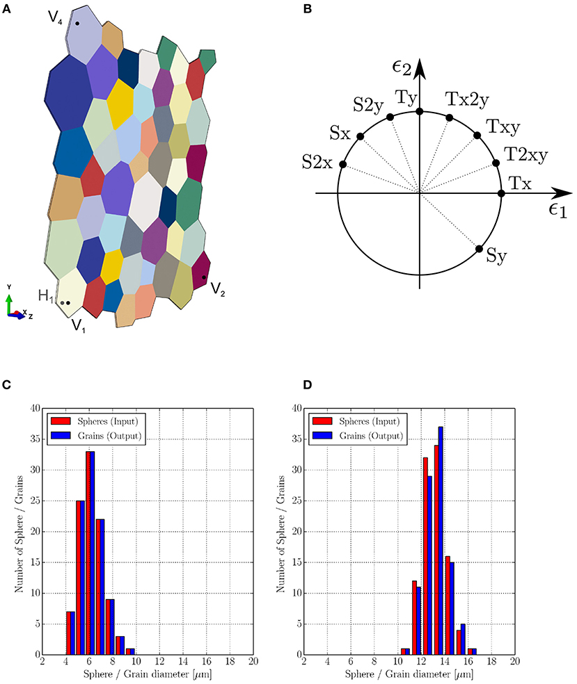
Figure 1. (A) Quasi-2D RVE with vertex nodes (V1, V2, V4, H1) needed for the boundary conditions (see section 2.3.3); RVE with a mean grain size of 59μm and a standard deviation of 10μm contains 51 grains between 40 and 90μm, has a side length of 348.8μm and a thickness of 1.7μm and is used as model for the damage evolution (cf. section 4). (B) Loading cases applied to the RVE used for the prediction the damage evolution in section 4. Comparisons of diameter distribution between defined spheres and constructed RVEs with (C) average grain size μ of 6.0 μm and standard deviation σ of 1.0 μm, and (D) average grain size μ of 13.0 μm and standard deviation σ of 1.0 μm.
2.2. Crystal Plasticity Model
The material behavior of the FE simulation is described by a phenomenologically based crystal plasticity model. To resolve the heterogeneous deformation resulting from abrupt changes in mechanical behavior across grain boundaries of the considered polycrystal and to consider size effects between small and large grains, a nonlocal crystal plasticity model proposed by Ma and Hartmaier (2014) is implemented. As the applied nonlocal crystal plasticity model is already described in Ma and Hartmaier (2014), only an overview of the formulation is given. For further details on the non-local flow rule, the reader is kindly referred to Ma and Hartmaier (2014). In the following, quantities written in bold letters refer to vectors (small letters) and matrices of second rank tensors (capital letters). From the kinematics of deformation, the total deformation gradient F can be multiplicatively decomposed into the elastic deformation gradient Fe and the plastic deformation gradient Fp,
The elastic deformation is calculated using the Hooke's law. The plastic deformation is characterized by the plastic velocity gradient Lp, which is a function of the plastic deformation gradient Fp and its rate as,
For this study, a crystallographic slip of dislocations is defined as the only mechanism for plastic deformation. Thus, Lp is taken as the sum of the shear rates of all slip systems,
Here, is the plastic shear rate. Mα = dα⊗nα is the Schmid tensor for slip system α, which is defined by the slip direction dα and the slip plane normal nα. The symbol ⊗ denotes the dyadic product of two vectors resulting in a second rank tensor. The total number of slip systems is N.
With respect to the nonlocal crystal plasticity model proposed by Ma and Hartmaier (2014), the flow rule and the hardening law can be expressed as:
and,
where, is the reference shear rate, and p1 is the inverse value of the strain rate sensitivity. Furthermore, h0 is the reference hardening parameter, χαβ is the cross hardening matrix, which is assigned as 1.0 for coplanar slip systems and 1.4 otherwise, is the saturation slip resistance, and p2 is a fitting parameter. The initial value of the slip resistance is defined as , and sgn() is a mathematical function that extracts the sign of a real number. The resolved shear stress τα for each slip system can be calculated from the stress Sα in the intermediate configuration or the state involving only the plastic deformation gradient Fp as,
The flow rule in Equation (4) consists of two additional back stresses and describing the hardening contributions from geometrically necessary dislocations (GNDs) (Ma and Hartmaier, 2014). The nonlocal constitutive model, in this context, is derived from the concept of super GNDs densities and incorporates the plastic strain gradient. Within a continuum mechanical approach, it is not possible to define crystallographic GND based on the Nye tensor in a unique way. To capture the internal stresses resulting from GND, the concept of super dislocations is followed, which allows us to define the dislocation Burgers vectors and line directions uniquely (Ma and Hartmaier, 2014). This hardening from plastic strain gradients is split up into an isotropic hardening part and a kinematic hardening part .
The second rank dislocation density tensor G in the reference configuration is computed from the curl of Fp as introduced by Nye (1953),
where Δjkl is the third rank permutation tensor and “l” represents the derivative with respect to the cartesian coordinate “l”. It must be noted that in Equation (7) the dislocation density tensor is written in index notation (G = Gij). Since a reconstruction of meaningful crystallographic dislocation populations in a unique way is impossible, a unique definition of super GNDs is obtained by projecting the dislocation density tensor to the global Cartesian coordinates of the system. As a result, the stress fields of the crystallographic GNDs can be described with a good accuracy (Ma and Hartmaier, 2014), and the GND density tensor can be segmented into nine independent parts by evaluating,
where dα and tα are permutations of the Cartesian unit vectors as determined in Ma and Hartmaier (2014), and b is the magnitude of the crystallographic Burgers vector. The super GND densities for α = 1, 2, 3 represent screw-type superdislocations, while the remaining 6 components represent edge-type superdislocations, which are vital for determining the internal stress fields as a consequence of the super GNDs.
The isotropic hardening for the dislocation slip contributed by these super GNDs can be expressed using a Taylor-type equation,
Here, c1 is the Taylor hardening coefficient or a geometrical factor [38], and μ is the shear modulus. is the cross hardening matrix between crystallographic mobile dislocations and super GNDs.
The long-range internal stresses, caused by GNDs in dislocation pile-ups, contribute to the kinematic hardening effect. This part is calculated by evaluating the second order gradient of Fp, which results in a super GND gradient ρα in the form,
By evaluating these gradients within a small volume of dimension L3, the internal stresses in the intermediate configuration caused by dislocation pile-ups at grain boundaries can be calculated as explained in Ma and Hartmaier (2014). Thus, the kinematic hardening can be given by:
For the FCC crystal structure, the dislocation slip on the common crystallographic 〈110〉{111} slip systems is considered. On the other hand, we only take the dislocation slip on the crystallographic 〈111〉{110} slip systems into account for the case of BCC crystal structure.
2.2.1. Damage Model
For the first application of damage homogenization using Machine Learning (ML), a formulation to compute the local damage is also needed in addition. This applies for the prediction of the damage evolution (cf. section 4). The damage of a material can be assessed by using the damage parameter D, which is defined as the ratio of the damaged volume to the initial volume (cf. Lemaître, 1985) and can, therefore take values between zero and one. The increase of damaged volume leads to a reduction of the stiffness of the material. In general, for an ideal isotropic and uniaxial case, the damage parameter, Dstiff, can be described in terms of the Young's modulus as,
where Einitial is the initial Young's modulus and the Edamage is the E-modulus after the damage occurred. More generally, both quantities can be interpreted as the material stiffness along a given loading path. In our model, the damage is calculated numerically using a ramp function, which depends on the equivalent plastic strain p. The equivalent plastic strain is computed as the Frobenius norm (Gentle, 2007) as,
where the subscript F indicates the Frobenuis norm, and Ep is the plastic Green-Lagrange, strain which is computed by using the plastic deformation gradient Fp (Haupt, 2002). The plastic deformation gradient is computed according to Equations (2) and (3) in section 2.2 using the plastic velocity gradient Lp, which depends on the shear rate and the Schmidt tensor Mα. After an initial threshold value of the plastic strain is reached locally, the damage increases linearly with the plastic strain. Once the upper limit of the plastic strain occurs, the damage parameter reaches its maximum value. Locally, the damage parameter is computed as follows,
p1 and p2 are the lower limit and the upper limit. In Figure 2, the damage model is given graphically. For values smaller than the lower limit of the plastic strain, the damage parameter equals zero. Hence, the damage parameter reaches its maximum value for plastic strains higher than the upper limit, which numerically is realized by setting the parameter close to, but not equal to, one (Dmax = 0.999). The damage evolution is the rate of the damage parameter. Here, the limits were chosen so that the resulting model reaches its uniaxial tensile strength at around 10% total strain: p1 = 0.3 and p2 = 0.5. Note that the limits were not chosen to describe a specific alloy.
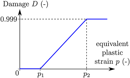
Figure 2. Local damage model for the numerical computation with p1 and p2 being the lower and upper limit defining the start and saturation of damage.
2.3. Homogenization Methods
In the previous section, the material model for the microscopic FE simulations was described. For the ML algorithms, homogenized values (or global values) that describe the RVE are used. In the following, the global homogenized parameters have the superscript RVE. The homogenization procedure is different for the two applications presented here (cf. sections 4 and 5). For the prediction of the damage evolution, the global values are homogenized according to the Hill-Mandel condition (Hill, 1963, 1972) in section 2.3.1 and with respect to the stiffness reduction in section 2.3.2. It is necessary to use such volume average technique, because the damage needs to be calculated locally. For the prediction of microstructural features from the flow curve, macroscopic stress and strain tensors are calculated with respect to the approach of Nemat-Nasser (Nemat-Nasser, 1999). In this case, we only need to formulate a macroscopic stress and strain tensor in order to calculate the flow curve. Therefore, we use a much simpler and numerically more effective efficient approach described in section 2.3.3. In this section, methods to homogenize global values or macroscopic properties from microstructure simulations are described.
2.3.1. Volume-Average Method
From the FE simulation, the value of each Gauss point is extracted, i.e., eight values for each element (cf. section 2.1). The bullets in brackets stand for the parameter that is homogenized, i.e., the stresses and strains. The Gauss point values of each element are averages, so one value for each element is obtained,
Here, the index Gauss refers to the current Gauss point, which can take values from one to eight. To obtain global representative values for each time step, the local values, which are the average values of the eight Gauss points, are averaged by using the element volume,
where the index e indicates the current element and Nel is the total number of elements. The symbol V is the volume, and VRVE is the total volume of the RVE. As Equation (16) shows, the global (homogenized) value is the sum of the local element value multiplied with the corresponding volume, which is then scaled by the total volume of the RVE. This averaging procedure is well established for stresses and strains (see Jänicke, 2010, Nguyen et al., 2012b) and is based on the Hill-Mandel condition (cf. Hill, 1963, 1972). Nevertheless, the application of Equation (16) is not appropriate to define a suitable measure for the homogenized damage state: consider a microstructure that is fully damaged, i.e., a crack with distinct width runs through the entire ensemble of grains. Then, the volume fraction of the damaged areas may be less than few percent of the entire microstructural volume. However, the microstructure is not able to sustain any load (in the direction that caused the damage evolution). Consequently, the usage of this small value for the volume-averaged damage state would underestimate a comparable measure according to Equation (17) for the effective damage state at the macroscale to a large extent: the volume average for the damage does not reflect the true physical properties of the microstructure. We thus propose a different homogenization scheme for the damage variable in the next subsection.
2.3.2. Homogenization of the Damage Variable
As indicated earlier, a homogenization of the damage variable via volume averaging is not appropriate for defining a reasonable measure for the effective damage state that can be used for a description of the macroscopic behavior. In the available literature some attempts have been made to solve this problem. Nguyen et al. developed a multiscale cohesive damage model to determine the macroscopic behavior of a quasi-brittle material. They homogenized the response of a microscale sample representing the heterogeneous microstructure inside the adhesive crack (see Nguyen et al., 2012b, Nguyen et al., 2012a). Fish and Yu derived a closed-form expression relating microscopic, mesoscopic and overall strain and damage (Fish and Yu, 2001) for brittle materials. These approaches are, however, applicable to the small strain regime and to brittle/semi brittle materials. Souza and Allen developed homogenization-based multiscale frameworks for impact modeling of heterogeneous viscoelastic material. The damage was modeled through a field of evolving microcracks using XFEM method and cohesive law. In the above mentioned approaches, the correlation between damage evolution and large plastic strain is missing. It was, hence, necessary to develop an approach which is also valid for large plastic strain regime (Souza and Allen, 2009). We, therefore, define a homogenization approach that is in accordance with the definition of the damage parameter (at the microscale):
where CD and C0 define the effective structural stiffness of the microstructure in the damage (subscript D) and the initial state (subscript 0). Consequently, DRVE has an identical meaning to the local definition of the damage variable according to (12). The important difference is, however, that Equation (17) accounts also for geometrical aspects. Thereby, DRVE depends on both the damage (evolution) and the microstructural arrangement provided by the specific microstructural composition, e.g., in terms of grain sizes, grain orientation and grain boundaries.
The values for the stiffness CD and C0 can be extracted from the equivalent stress σeq for equivalent elastic strain (both scalar-valued quantities): The equivalent strain results from volume averaging of the local elastic strain components, following from local total strain and the local plastic parts as function in time. In a comparable manner, the equivalent stress results from the volume averaging of the stress distribution. Then, the initial stiffness is defined by:
and for the damaged stiffness we define accordingly:
The initial stiffness represents the stiffness of the undamaged state, indicating that the tuple can be read off the equivalent stress/equivalent strain curve at any load step before damage sets in. For this case, the initial stiffness was computed as the slope between the first stress/equivalent strain point and the point corresponding to the maximum stress. The damaged stiffness CD evolves in time as the fraction between and is no longer constant (in contrast to C0): the crack evolution at the microscale renders the volume-averaged equivalent stress being a monotonously decreasing function such that lim CD = 0, whereas CD = C0 just before damage sets in. Accordingly, DRVE ∈ [0, 1], where DRVE = 0 indicates a completely intact and undamaged microstructure, whereas DRVE = 1 represents a completely damaged microstructure. Consequently, this measure can be used for future applications of our approach presented here: the microstructural behavior is computed for reference states on which the machine-learning algorithm is built. This results in an effective material model for the simulation at the macroscale while taking into account the microstructural effects that are synthesized in the effective damage parameter DRVE. The macroscopic damage evolution is computed as the change of the homogenized damage parameter 〈D〉 with respect to the time, t, according to,
where, n indicates the current time step. Note that we apply this homogenization approach only for monotonous loading paths in this work.
2.3.3. Homogenization of Macroscopic Stress and Strain Tensors From Periodic Boundary Conditions
With respect to periodic boundary conditions applied to the RVE, the global deformation is imposed to the four reference nodes, V1, V2, V4, and H1 as highlighted in Figure 1A. The RVE boundary nodes are imposed on the kinetics of these reference nodes. Therefore, macroscopic quantities can be homogenized directly from nodal displacement, reaction force, and position vector of these reference nodes as introduced in Kulosa et al. (2017). For further details on the implemented homogenization technique, the reader is kindly referred to Boeff (2016); Kulosa et al. (2017). The macroscopic strain tensor can be formulated from the nodal displacement and be mathematically expressed as:
Δx, Δy, and Δz are dimensions of the periodic box in the global Cartesian coordinate system. Similarly, the macroscopic stress tensor can be formulated from the reaction force vectors Fnode at the four reference nodes and the current nodal position vectors xnode of the reference nodes which is given as:
The symmetrization function is defined as sym=1/2[A+AT] for tensor A and its transpose. With the formulated macroscopic stress and strain tensor, the von Mises stress (σvM) and equivalent plastic strain (p) can be calculated accordingly.
3. Machine Learning
This section gives a short description of the types of supervised learning algorithms used in this work. In case of supervised learning (as opposed to unsupervised learning), the actual output is known and has to be approximated by the algorithm. In general, the algorithm learns to predict the target output for given features (input parameters) with a minimal error by adjusting parameters. A function y(x) is created by the Machine Learning (ML) algorithms, where y is the predicted output depending on the input features x. In general, the input and output are vectors, their length depending on the given problem. Here, for both applications (predicting the damage evolution in section 4 and predicting the grain size from the flow curve in section 5), there are several input features, so that the input is a vector. However, the output is a single scalar quantity. Furthermore, the target values are real-valued and known, and therefore supervised regression algorithms are used. For both cases, Support Vector regression (SVR) and Random Forest regression (RFR) algorithms are used. In this section, both algorithms (sections 3.1 and 3.2) are explained briefly with respect to regression.
3.1. Support Vector Regression
Following the work of Hastie et al. (2008), SVR is an extension of linear regression and used for non-linear problems. In the following, the theory of SVR is briefly described. A more detailed description can be found in Appendix 7.3. The main idea is to gain a function fitting the given data points so that all points lie within a (small) distance of ϵ to the function (see Figure 3A). In Figure 3A, a simple two-dimensional problem is shown, in which all data points are supposed to be described by a linear function. The green area is called the margin, and its width is equal to two times ϵ. To obtain the best fit, the main task is to minimize the margin, and for doing so to solve a convex optimization problem (cf. Smola and Schölkopf, 2004; Hastie et al., 2008). Furthermore, so-called slack variables ξ are introduced, for measuring the relative distance by which the target distance of ϵ is violated (cf. Figure 3A). The points far away from the margin are the so-called support vectors. In addition, a regularization or cost parameter C is specified. It balances the contradictory goals of a good fit vs. a simple model by weighting the penalty for the slack variables. Furthermore, outliers have more influence in shaping the predicted output. To enable the algorithm to develop complex non-linear functions, so-called Kernels are introduced (Ng, 2016). Kernels are customizable to the needs of the target domain, which gives the algorithm the advantage to be adaptable to many problems. With the kernel function, it is possible to map the input data into an enlarged feature space. Since this mapping is in general non-linear, kernels enable SVRs to represent highly non-linear functions. In this work the Gaussian radial basis function kernel:
is used (Müller and Guido, 2017). The parameter γ controls the width of the Gaussian kernel. The decision function is then no longer linear, but rather a flexible weighted sum of Gaussian kernels.
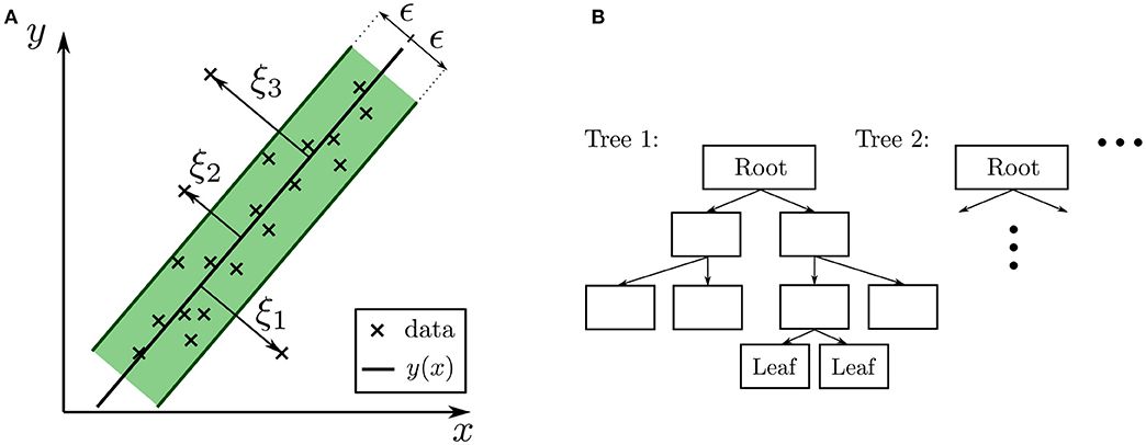
Figure 3. Illustration of the Machine Learning (ML) regression models. (A) SVR: example of a two-dimensional problem as described in section 3.1 with the margin of two times ϵ and slack variables ξi (B) RFR: example of Decision Tree (Tree 1) with depth three (cf. section 3.2).
3.2. Random Forest Regression
RFRs are a combination of multiple Decision Trees (DTs) or, more precisely in our case, regression trees. It is a prototypical ensemble method, which builds a highly accurate predictive model by combining many simple models (often referred to as weak learners). Each DT predicts an output, and their results are averaged. DTs are hierarchy-based models where the goal is to find the right answer by “asking as few if/else questions” as possible (Müller and Guido, 2017). For regression, nodes contain the distinction whether a value is below or above a threshold value. The main idea is to split the feature space into regions using recursive binary partitioning (cf. Hastie et al., 2008), so that every new data point can be assigned to one region. A visual example of a RFR is given in Figure 3B. Here, the single DT has a so-called depth of two. The tree depth is equal to the longest number of consecutive nodes in a tree. Every DT starts with a root (the top node), which contains the first question, e.g., whether a chosen feature of the data point is smaller or larger than a specific value. The nodes of the last layer of the tree are called leaves. Each leaf corresponds to one target value, i.e., a single value of the output domain. Each data point is assigned to exactly one leaf by following the decisions down the tree. If a leaf contains only data points that correspond to the same target value, the leaf is called pure. Using DTs with pure leaves results in a model that can fit the training data perfectly, but can result in over-fitting. There are four important algorithm parameters that are tuned for the RFR in this work (cf. Müller and Guido, 2017). The number of used DTs (estimators) influences the amount of over-fitting and also the computation time. In addition, the maximum depth of each tree can be chosen specifically, or the tree is built until each leaf is pure or reaches a minimum number of samples inside the node. Furthermore, a criterion to decide whether to split a node needs to be defined, e.g., mean squared error. Another important parameter is the maximum number of features used for splitting a node. In general, a low value of this parameter means that each tree is different and may not need to be deep enough to be sufficiently accurate. A high maximum feature parameter or setting the value equal to the total number of features, results in DTs that are quite similar and thus defeating the purpose of an ensemble in the first place. The training data are fitted well by building deep trees and using the most distinctive features.
4. Homogenize Damage Evolution From Micro- to Macroscale
As mentioned in section 1, a new method to map damage from the micro- to the macroscale using Machine Learning (ML) is proposed. Based on the described representative volume element (RVE) (cf. section 2.1) and the local crystal plasticity model (cf. section 2.2) with damage (cf. section 2.2.1), several finite element (FE) simulations using Abaqus (version 6.12–3) are conducted. Here, the local crystal plasticity model is used, hence no influence of the geometrically necessary dislocations GNDs is considered. The main aim of the damage evolution application is to show that the global material response, gained from FE simulations, can be generally approximated with ML algorithms. For this application, we do not compare results obtained with different meshes. The material parameters are given in Table 4 in the Appendix 7.1. First, the data set for the ML algorithms is explained (cf. section 4.1), then the ML parameters are presented (cf. section 4.2). Finally, the results are given in section 4.3. Note that all parameters, such as stresses and strains, are the global, hence homogenized (cf. section 2.3), parameters. For simplicity reasons, the superscript RVE of the global parameters are skipped throughout the current section 4.
4.1. Data Set
A variety of loading states are simulated to make the data base valid for damage occurring under general monotonous loading paths. Hence, nine displacement-controlled simulations with different loading states are performed: uniaxial tension, biaxial tension cases, and shearing as shown in Figure 1B. The nine loading cases are uniaxial tension in x- (Tx) and y-direction (Ty), biaxial tension Txy, T2xy, and Tx2y (see Figure 1B). In addition, four shearing cases were applied: Shearing in x- (Sx, S2x) and y-direction (Sy, S2y) according to Figure 1B. The RVE used for the creation of the data set for ML is presented in Figure 1A in section 2.1. It contains 51 grains with a mean grain size of 59μm and a standard deviation of 10μm, which results in a grain size range between 40 and 90μm. The material model, as well as the damage model and the homogenization methods, are described in sections 2.2 and 2.3, respectively. First, the local results are presented. Then the global material behavior is presented. As an example, Figure 4 shows contour plots of the von Mises stress and the damage parameter for uniaxial tension in x-direction.
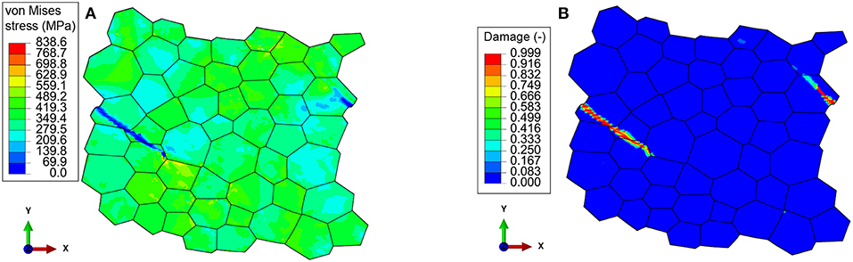
Figure 4. Contour plot of the (A) von Mises stress and (B) damage parameter for uniaxial tension in x-direction at about 14.3% total strain.
In both Figures 4A,B, a strain localization in form of a band can be seen inside the RVE. Note that the damaged zone is split up because of the periodic boundary conditions. It is due to such a morphology of the damage band that a new homogenization scheme is required to homogenize it from the micro to the macro-scale (see section 2.3.2). At the flanks of the localization band, the stress is close to zero and the damage parameter has reached its maximum of 0.999. Furthermore, it is noted that the damage band propagates through the grains, i.e., in a transgranular manner, as one would expect for a ductile material, where damage and fracture occurs by void nucleation, coalescence and growth. From the simulations, relevant parameters for the homogenization are extracted: equivalent total, elastic and plastic strain, equivalent plastic strain rate, von Mises and hydrostatic stress, as well as the element volume. Locally, the parameters are computed as follows: The equivalent plastic strain is computed as described in section 2.2.1 and its rate is computed equivalently to the rate of the damage parameter according to Equation (20). The equivalent total and elastic strains are computed in the same way as the equivalent plastic strain using the Frobenius norm and the Green-Lagrange strain (cf. Equation 13). The total deformation gradient F is calculated as the gradient of the displacement, and the elastic deformation tensor is computed as Fe = FFp−1 (Haupt, 2002). The von Mises and hydrostatic stress are computed according to Gross et al. (2011). The extracted values are homogenized as described in section 2.3.1 and 2.3.2: The global stress and strain values are the volume average of the local (element) values, and the global damage is calculated based on the stiffness reduction of the entire RVE. This results in eight global parameters: equivalent plastic strain (p) and its rate (), equivalent total () and equivalent elastic strain (), von Mises stress (σvM), hydrostatic stress (σhyd), and the damage parameter (D) and its rate (). After the homogenization, a further pre-processing of the points is applied (see Appendix 7.2), which spaces the data equally with respect to the equivalent plastic strain. Each data point represents one time step of the FE simulation. For each time step, there is a set of parameters consisting of the global parameters previously mentioned. Therefore, the complete data set has the size 9 × (●) ×8, where (●) is the number of time increments for each of the 9 loading cases applied to the single RVE (cf. Figure 1A), and 8 is the number of global parameters (p, , σvM, σhyd, , , D, ). In total, the time increments of all loading cases equal 3454. For all data points used in this application, the reader is kindly referred to Data Sheet 1_v1 in the Supplementary Material. The global values are used as the data set for the training and testing of the ML algorithms. The number of training and test data has been verified to be sufficient by using so-called learning curves, which are further described in section 4.2. The global material response in terms of the von Mises stress and damage rate with respect to the equivalent total strain can be seen in Figures 5A,B. The global behavior is given in the following by showing five out of the nine loading cases with the most significant difference in the material response.
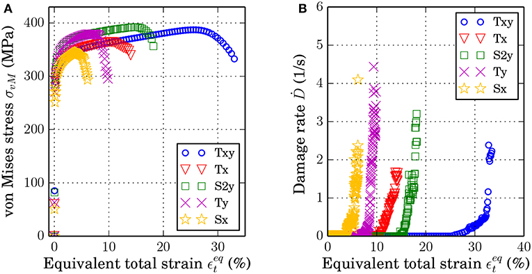
Figure 5. Global data plots for uniaxial tension in x- and y-direction (Tx, Ty), biaxial tension (Txy), and shearing in x- and y-direction (Sx, S2y): (A) von Mises stress plotted against the total equivalent strain, (B) Damage rate as a function of the total equivalent strain.
It can be seen in Figures 5A,B that different loading conditions result in (quantitatively) different stress and damage evolution, although the general curve shapes are (qualitatively) similar. Each loading condition shows a distinct starting point for the initiation of damage, which corresponds to the maximum stress occurring at different global strains. In addition to the given global plots, it is worth having a look at the maximum global damage parameter. For the uniaxial and biaxial tension, the value is quite similar: 35.77% of maximum global damage for biaxial tension (Txy), and 35.78 and 37.7% for uniaxial tension in x-direction (Tx) and y-direction (Ty), respectively. The two shearing cases Sx and S2y have a lower maximum value for the global damage parameter. For shearing in x-direction (Sx), the maximum global damage occurring is 24.86%, and for S2y it is 27.18%. It should be noted that even though the tension cases share a similar maximum global damage value, the evolution of damage, with respect to the total equivalent strain, is different as seen in Figure 5B. In the following, the ML models and their parameters are presented.
4.2. Machine Learning Models and Parameters
For this application, Support Vector regression (SVR) and Random Forest regression (RFR) are used to predict the damage evolution . The ML is conducted using python and scikit-learn 0.19.1 (cf. Pedregosa et al., 2011). The data set is split into training (75%) and testing (25%) data sets. For validation, the training set with 75% of the data is used as the “complete” data set, and therefore further split into a training set (for validation purposes) with 56.25% of all data points, and a validation set with 18.75% of the data. The testing and validation data set is unseen data that is only used for evaluating the final model, i.e., after the final ML parameters are set. The validation set acts as a test set during the fitting of the ML parameters. Before splitting the data into sets, the order of the data was randomized in a way that can be reproduced (constant random state of 666 Müller and Guido, 2017, Pedregosa et al., 2011). To assess the accuracy of the learning algorithms, the so-called R2 score is used (Müller and Guido, 2017), which is computed as a fraction of the mean squared error and the variance (Pedregosa et al., 2011),
Here, y represents the output vector, index true indicates the reference output data, true, mean the mean value of the reference output data, and index pred represents the output data predicted by the ML algorithm. The total number of data points is assessed to be sufficient by using learning curves (cf. Ng, 2016) and cross-validation. Learning curves are a tool to check whether the number of data points used for training and testing is sufficient (Pedregosa et al., 2011). The training data is split several times into different set sizes to see the development in training and validation score with respect to the number of data used. Here, RFR is used to train and validate the model since its training process is very robust and shows only little sensitivity to the training parameters. As mentioned in section 4.1, a total number of 3454 data points are available. For the training and validation, 56.25 and 18.75% of the data is used, i.e., 2071 (training) and 519 (validation) data points, respectively. The training data is split seven times, so that the following absolute training split sizes result: 207, 517, 828, 1139, 1449, 1760, 2071. The validation set is 20% of each split. The resulting training and validation scores converge after using 1449 training data points to 97.3–97.5% for training and 82.3–82.8% for validation. Selecting the most predictive subset of features can help to avoid over-fitting. Therefore, the features were chosen according to conducted feature importance methods and to an ductile damage model from the literature (cf. Equation 25), which is formulated in a mathematically closed form as analytical function. Feature importance is used to assess the influence of each feature with respect to the result. The attribute importance can be understood as a value of how informative each feature is and therefore shapes the result. For the feature importance, RFR is used (cf. section 3.2) with the only non-default parameter being the number of Decision Tree (DT) (=500). Note that feature importance gives a rank of all features with respect to their impact on the results. Less important features are not necessarily trivial, and neglecting them does not automatically improve the results. Nevertheless, feature importance can provide an understanding of the relationship between input and output parameters with respect to the ML algorithms. As mentioned above, the training data contain 56.25% of the data, and the validation set accounts for 18.75% of all data points. The other 25% of the data is the test set, i.e., the unseen data that is only used after the training process to assess the ability of the ML algorithm to generalize. As mentioned in section 4.1, for the feature importance all extracted features are used without additional polynomial features or interactions. The results of the feature importance are presented in a bar plot in Figure 6.
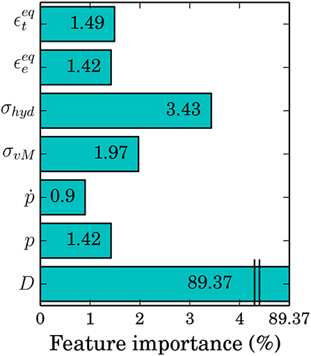
Figure 6. Results of the feature importance presented in a bar plot showing the importance of each feature in percent. Here, the x-axis is only properly shown up to 4% for clarification because all features, except for the damage parameter, show values < 4%.
The conducted feature importance results in the damage parameter being the most informative feature with a validation score of 89.37%. This leaves the importance of all other features to around 10% in total with 3.4% for the hydrostatic stress being the second most relevant feature, and the plastic strain rate the least important feature with 0.9%. Selecting half of the most important features (D, σvM, σhyd, ) produces a validation score of about 94.58%. One can see that the damage parameter and the stresses seem to be the most relevant, based on feature importance. For the RFR, selecting only the most relevant features (D, σvM, σhyd, ) leads to better results than other feature combinations. In contrast, these input parameters induce a lower accuracy for the SVR. Choosing the same features for SVR as chosen for RFR, results in a training score of just about 77.6% and a test score of 82.2%. Both score values are below acceptance. The SVR cannot extract enough information from the given features to approximate the damage rate sufficiently. Therefore, leaving out features causes an under-fitting problem so that all features are used: D, p, , σvM, σhyd, , . Taking a look at the analytical ductile damage model,
one can see a similarity in the input parameters compared to the results of the feature importance (Chaboche, 1988; Ambroziak, 2007). In the above Equation (25), s and S are material damage parameters. In addition, constant material parameters such as the Young's modulus [E = 228.96(GPa)] and Poisson's ratio [ν = 0.27(−)] are used, which can be calculated from uniaxial stress and strain curves. The input parameters for the analytical damage model are similar to the selected parameters by the feature importance, damage parameter and stresses. Later, the ML results are compared to the analytical damage model given in Equation (25) to investigate whether ML algorithms can describe the damage evolution at least as well as a well-established closed-form damage model.
Furthermore, cross-validation is used to find the best ML parameters. First, the most appropriate method to scale the data is determined for the SVR (as RFR does not require a scaling of the data). The input data are scaled according to a Gaussian normal-distribution with zero mean value and a variance of one (standard scaler Pedregosa et al., 2011). Moreover, cross-validation is used to assess the most suitable kernel and whether to use additional polynomial features. In this case, the Gaussian kernel and no additional polynomial features result in the highest accuracy. Furthermore, grid-search, i.e., finding a parameter set that results in the highest accuracy, is used to find the best parameter value of the regularization parameter C (cf. Equation 25) and the Gaussian kernel coefficient γ (cf. Equation 32). During grid-search, both parameters are fitted simultaneously. Here, the epsilon-SVR model is used, which is named after the parameter ϵ which can be found in Equation (28) of the Appendix 7.3. This precision parameter defines the distance between data point and target value, which is still considered accurate, and has no negative influence on the overall accuracy (Pedregosa et al., 2011). For the RFR, the cross-validation is used to choose the best number of DTs, the maximum tree depth and the split criterion of a node. A number of 500 DTs gives the best results with respect to a reasonable compromise on the computation time. Each DT is built until all leaves are pure, i.e., each last node corresponds only to a single target value, and the criterion to split a node is the mean absolute error. In Table 1, the optimum parameters of both ML algorithms are summarized. The other parameters, as defined in the scikit-learn library (Pedregosa et al., 2011), are set to their default values. RFR is rather robust with respect to the parameter values. Generally, SVR is more sensitive to parameter tuning. Therefore, its parameters were tuned within a smaller range. Within this range, the SVR parameters are not as sensitive to tuning. For example, changing the values for the parameters C and γ from their optimized values (based on the Grid-Search method) by 10% changes the training score by about 0.02% and the test score by around 0.04%. With the described data set and the fitted ML parameters, the two algorithms are trained. The results of the training processes are given in the next section 4.3.
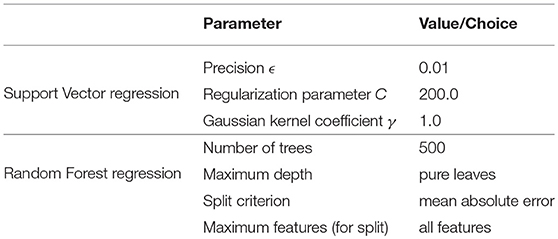
Table 1. ML parameters used for SVR and RFR (scikit-learn library, cf. Pedregosa et al., 2011); Other parameters are default values.
4.3. Results and Discussion
For the homogenization of damage, two algorithms are used: SVR and RFR. The same randomly partitioned data set for the training and the testing process is used for both algorithms. The final training processes are conducted by using the previously defined parameters (cf. Table 1) and by using the features that lead to the best results as described in section 4.2. For SVR the training and testing processes both have a considerably high accuracy: 99.73% (training) and 98.25% (testing). One can see that the high accuracy for training as well as testing indicates no over- or under-fitting (high bias or high variance) problems. The same applies for the RFR: the training score is 97.66%, and the test score is 97.48%. The results of the algorithms are presented in Figures 7A,B. In both cases, only the testing data set (25% of all data) is displayed in the form of a predicted data against the target damage rate plot. The red lines in both figures represent the 5% mismatch area calculated based on the R2 score (see Equation 24). Here, the predicted data are the output of the ML algorithm, and the real data are the reference damage rate gained from the simulations.
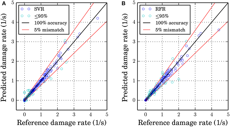
Figure 7. ML results of the test set (25% of the data) with predicted values plotted against target values, a ±5% mismatch border (red line) of the R2 score and points with a lower or equal R2 score of 95% (cyan color) (A) SVR with a score of R2 = 98.25% (B) RFR with a score of R2 = 97.48%.
From the data set, one can see that the majority of data points have damage rate values below 1/s. Hence, the damage evolution is predicted more accurately for such values. Even though, both algorithms have a sufficiently high accuracy on the test set, the SVR is able to approximate the damage rate more accurately for higher damage rates. SVR lacks to approximate the damage rate sufficiently for values near zero as one can see in Figure 7A, where a reference damage rate of around 0.3/s is predicted for one point. The RFR has a lower accuracy for larger damage rate values but can approximate values near zero more accurately than the SVR. Some data points were predicted incorrectly with an error of more than 5% for both algorithms, but the SVR shows less scattering inside the ±5% mismatch area. Furthermore, the SVR is able to predict high values for the damage rate more precisely than the RFR.
In Figure 8A, the ML algorithm results are given in a damage rate against equivalent total strain plot for five loading cases. Both ML algorithms are able to capture the damage evolution with increasing strain, even though not every value can be predicted perfectly. Hence, the ML algorithms are capable of predicting the damage evolution for different loading states precisely. In general, the ML algorithms can approximate the material response with respect to damage behavior almost as well as the full-field FE simulations as shown in Figures 7, 8. The comparison of the trained ML algorithms to the analytical damage model is given in Figure 8B for the test data points for the uniaxial tension in x-direction. For the analytical damage model, the two material parameters had to be adjusted: s = 5.06(−) and S = 0.24(MPa) (cf. Equation 25). Both, SVR and RFR, are trained as described previously and shown in Figure 7. The ML algorithms are able to describe the damage evolution well as mentioned above. Nevertheless, SVR shows a slight over-fitting problem as the damage rate marginally decreases after the maximum of around 1.58(1/s) (cf. Figure 8B). One can see a small roughness in the course, but no over-fitting is visible for the RFR. Consequently, the RFR method is more robust to describe the damage evolution for the presented cases than the SVR method. Furthermore, the fitting of the algorithm parameter is less demanding for RFR compared to SVR. The analytical damage model is able to describe the general damage evolution (see blue line in Figure 8B). Nonetheless, some limitations for the analytical model are worth noting. According to the analytical model, a damage evolution is visible even before the actual damage initiation occurs (after about 10% of total strain). The reason for this is that in the numerical model we explicitly gave the limit of the strain value as the initiation criteria, while the damage evolves in the analytical model as soon as plasticity occurs; however, due to the selection of parameters it stays small until some level of plastic strain is reached. After the actual damage initiation, the analytical damage model also shows a gradual increase, although, some difference is observed between analytical model and the numerical simulations regarding the point of sharp increase in damage. Moreover, the analytical model is compared to only one loading state, and its generalization to a variety of loading states would require re-adjusting its material parameters. Furthermore, the analytical model does not allow to take microstructural quantities into account.
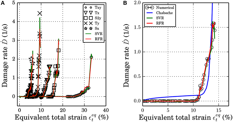
Figure 8. ML results with numerical data, SVR and RFR results plotted in a damage rate against total equivalent strain plot (A) for different loading states: uniaxial tension in x- and y-direction: Tx and Ty, biaxial tension: Txy, shearing in x- and y-direction: Sx and S2y (Numerical data points before damage initiation are not plotted) and (B) compared to the analytical damage model according to Equation (25) with the parameters s = 5.06(−) and S = 0.24(MPa) for the test data of the uniaxial tension in x-direction.
5. Property-Based Design of Microstructures
With the micromechanical modeling approach, the influence of important microstructural features on the mechanical response can be investigated through numerical simulations, yielding microstructure-property relationships. Thus, it is possible to use synthetical microstructures in form of representative volume elements (RVEs) together with their homogenized mechanical response that result from micromechanical simulations as training data for Machine Learning (ML) algorithms. Consequently, the input parameters of ML models are the required mechanical properties, and these trained models shall recommend microstructures that posses such properties accordingly, which represents one way of microstructure design.
5.1. Virtual Mechanical Testing of RVEs
In a first step, 74 RVEs consisting of 100 grains with various grain size distribution parameters following a log-normal distribution function were generated using the dynamic microstructure generator (DMG) introduced in section 2.1. In this context, the average grain size μ and the standard deviation σ are varied between 6–13 and 0.1–1 μm respectively. To exclude any influence of crystallographic orientation on the deformation behavior of RVEs, 100 different sets of randomly chosen Euler angles have been assigned to all RVEs. In this way, the remaining factor influencing the strain hardening behavior must be the grain size distribution parameters of the microstructure. In the next step, the nonlocal crystal plasticity model described in section 2.2 is implemented onto a user-defined material model (UMAT) and applied in a finite element (FE) simulation with the commercial software ABAQUS to assess the mechanical response of RVEs. By using a nonlocal crystal plasticity model, size effects including the influence of grain size are taken into account. For this part of the study, a BCC crystal structure is assigned to all grains in the RVEs; nonlocal crystal plasticity parameters are summarized in Table 4 in the Appendix 7.1 (Vajragupta et al., 2017).
5.2. Homogenization of Empirical Hardening Law
In the next step, the mechanical response of RVEs is simulated under a uniaxial tension loading condition, and macroscopic flow curves are homogenized from reference nodes using the method introduced in section 2.3.3. Examples of two RVEs with different grain size distribution parameters and the corresponding homogenized flow curves are shown in Figure 9. With a nonlocal crystal plasticity model, the influence of the grain size on the strain hardening behavior can be observed. These results prove the validity of implemented strain gradient crystal plasticity model and demonstrate that grain size effects can be incorporated properly in microstructure simulations. For the sake of simplicity, these flow curves are fitted with an empirical isotropic hardening law in order to reduce the dimensionality of the training data. In this context, the modified Voce law (Kim et al., 2013) is chosen and expressed as,
Y0, R0, Rinf, and β are material parameters to be determined, and p is the equivalent plastic strain. To parameterize the aforementioned hardening law from results of RVEs simulations, the nonlinear least square fitting method is implemented (Bates and Watts, 1988). As a result, two sets of calibrated modified Voce isotropic hardening parameters from two selected RVEs simulations are used to plot flow curves as illustrated in Figure 9. From the comparison, both fitted flow curves are in a good agreement with simulation results and can be used to represent microstructure simulations. Furthermore, the evolution of these fitted material parameters with respect to the average grain size is plotted as shown in Figure 10.
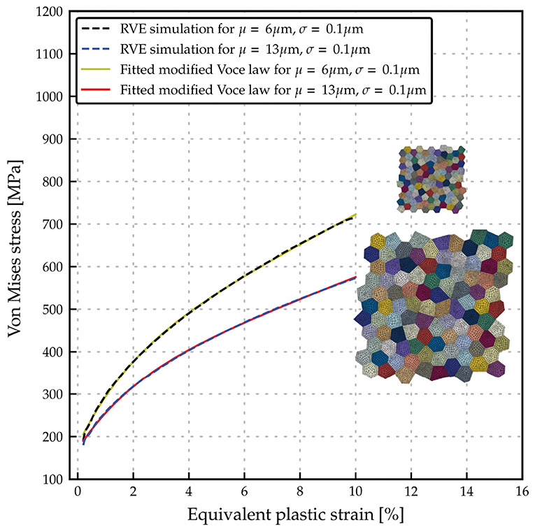
Figure 9. Flow curves comparison between 2 RVEs with different grain size distribution parameter and corresponding flow curves plotted using fitted modified Voce law parameters.
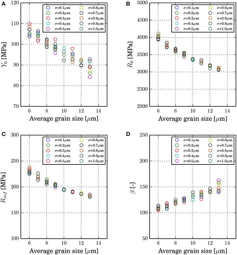
Figure 10. Influence of the average grain size on fitted material parameters of the modified Voce law (A) Y0, (B) R0, (C) Rinf, and (D) β.
From Figure 10, the influence of the average grain size on fitted material parameters of the modified Voce law is observed. According to Equation (26), Y0 is directly related to the yield stress. Fitted Y0 as plotted in Figure 10A linearly decreases with an increasing average grain size, and standard deviation influences a scatter of Y0 at the same average grain size. From Figures 10B,C, R0 and Rinf non-linearly decrease with larger average grain size. These two parameters behave similarly to the Hall-Petch relation. However, the standard deviation does not contribute to a scatter of R0 and Rinf. β, which inversely governs the slope of the hardening law and increases with an increasing average grain size. With respect to the hardening law, smaller average grain size results in a more pronounced strain hardening behavior. In the next step, these microstructure simulation results are fed as training data for ML models.
5.3. Training of Machine Learning Models
For this application, Support Vector regression (SVR) and Random Forest regression (RFR) are implemented to predict the average grain size producing a given material behavior, which is described by the parameters of the modified Voce hardening law. SVR and RFR are performed using Python and scikit-learn 0.19.1 (Pedregosa et al., 2011). The data are split into training (80 %) and testing (20 %) data sets. Similar to section 4, the R2 score is used to evaluate the performance of ML models. To determine hyperparameters of selected ML models yielding the highest accuracy, Grid-Search with 3-fold cross validation is applied, which manually considers all combinations of hyperparameters in a search space.
In Table 2, the optimized parameters of both ML models are summarized while other parameters as introduced in the scikit-learn library (Pedregosa et al., 2011) are set to default values.
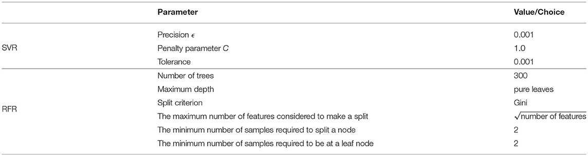
Table 2. Optimized ML parameters of SVR and RFR (scikit-learn library, cf. Pedregosa et al., 2011) for prediction of microstructural features from flow curve.
5.4. Results and Discussion
The training processes of both ML models for predicting the grain size from the flow curve are performed by using the defined parameters (cf. Table 2). For SVR, both, training and testing processes, give a high accuracy of 99.39% (training) and 97.95% (testing), respectively. These results indicate no over- or under-fitting issues. Similarly, trained RFR also results in a great accuracy for both training (99.62%) and testing (97.86%). The results of algorithms for the test data set (20% of all data) in the form of predicted grain size vs. reference grain size are shown in Figure 11. In this case, the predicted grain size data are the output from ML models and the reference grain size data are the grain sizes of RVEs used in microstructure simulations. From Figure 11, most of the data points from both trained ML models are within 5% error and there are only some data points, which give more than 5% error. Therefore, it can be concluded that there is no significant difference between both models in terms of scatter from the 100% accuracy line.
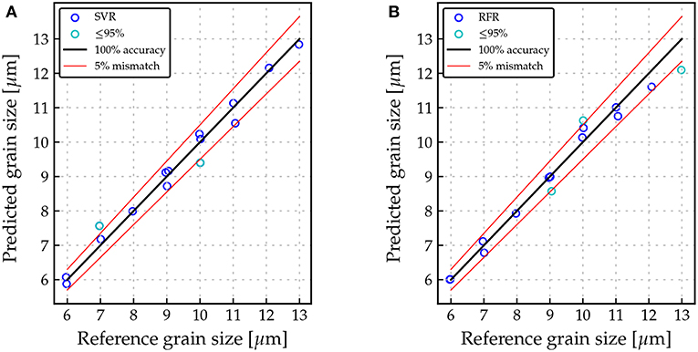
Figure 11. ML results of the test data set (20% of the data) with predicted grain size vs. reference grain size and a ±3% mismatch border (red line): (A) SVR; and (B) RFR.
Furthermore, trained ML models are tested with data that are out of range of the training data. In this context, an RVE consisting of 100 grains with average grain size of 15 μm and a standard deviation of 0.1 μm are generated using DMG. Plastic behavior is again described with a nonlocal crystal plasticity model, with parameters given in Table 4 in the Appendix 7.1, and uniaxial tension loading conditions are simulated. This microstructure simulation is homogenized to obtain macroscopic flow curves and modified Voce law parameters are determined using the non-linear least square fitting method accordingly. The fitted modified Voce law parameters are summarized in Table 3. For the validation process, these parameters are then used as input for both trained ML models to determine the average grain size.
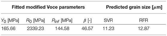
Table 3. Summary of fitted modified Voce parameters from microstructure model with the average grain size of μ=15.0 μm and σ=0.1 and predicted grain size using trained ML model.
By comparing the average grain size of the RVE to produce the flow curve with grain sizes predicted from ML models, significant deviations are observed when out-of-range-data are used, because predicted grain sizes are always within the range of training data. Therefore, such results show that an application of these trained ML models are only valid when the input data are within a certain range. Furthermore, it must be verified that the output data lie within the space covered by the training data. To further improve accuracy and to extend applicability of trained ML models, more training data covering a wider range of grain sizes should be used. In any case, within the range of training data, predicted grain sizes are still in a very good agreement with the reference data.
6. Conclusion
In this work, two novel applications with respect to using Machine Learning (ML) in material science were given and discussed. Both included microstructurally informed representative volume elements (RVEs) and crystal plasticity material modeling and used finite element (FE) simulations to study the mechanical response of different microstructures to applied loads. The results of the FE simulations were used to train and test the ML algorithms.
The first application was the approximation of damage evolution in an RVE using Support Vector regression (SVR) and Random Forest regression (RFR). Furthermore, their results were compared to the analytical damage model, which was formulated in a mathematically closed form as analytical function. The FE simulations included several loading conditions to be generally valid for monotonous load paths. The data gained from the simulations were homogenized and pre-processed before being used as training data for ML algorithms. Both regression schemes succeeded to predict the damage evolution correctly, with an accuracy (R2 score) higher than 97% on the test data set. Additionally, both algorithms were able to predict the damage rate for different loading conditions appropriately. Comparing the results of ML to the analytical damage model, the limitations of such an analytical model became visible. Both ML methods, SVR and RFR, were able to describe the damage evolution of a microstructure with very good precision. However, for the prediction of damage evolution, SVR showed a lower ability to generalize to unseen data than RFR and, furthermore, RFR shows a lower over-fitting problem, and its parameters are easier to calibrate.
It is observed that damage homogenization with ML algorithms exhibits several interesting features that are also observed in real experiments and macroscopic modeling, e.g., the shape of the damage evolution curve over the total equivalent strain or the fact that once damage is initiated, the increase in plastic strain leads to a sharp increase in the damage rate. These investigations show the capabilities of this method to predict macroscopic damage such that in future macroscopic applications, like deep drawing or sheet bending, it will become possible to include microstructure information into the constitutive relations of the materials.
The second application of ML methods aimed at predicting the necessary grain size in microstructure models to produce given flow curves with a desired work hardening behavior. This was accomplished, again, by using SVR and RFR. In this context, 74 RVEs with various grain size distribution parameters were generated, simulated for uniaxial tension and homogenized to obtain macroscopic flow curves. These simulated flow curves were fitted with a modified Voce law and the obtained parameters together with grain size distribution parameters of RVEs were used as input for the ML algorithms. For both ML models, the grain size prediction gave a good accuracy with R2 scores higher than 97.8% on the test data set. However, when out-of-range data were applied to trained ML models, predicted grain sizes strongly deviated from the reference quantities. It is hence concluded that the trained ML models are restricted to the space covered by training data. To further enhance the prediction accuracy, training data should cover a wider range of grain sizes. In any case, with a proper range of training data, one can see the prospect of using ML models to suggest microstructural parameters that produce desired mechanical properties.
Author Contributions
DR and KN performed the numerical simulations. AH, TG, and PJ defined the research scope. HuH and NV contributed to the paper writing.
Conflict of Interest Statement
The authors declare that the research was conducted in the absence of any commercial or financial relationships that could be construed as a potential conflict of interest.
Acknowledgments
We acknowledge support by the DFG Open Access Publication Funds of the Ruhr-Universität Bochum.
Supplementary Material
The Supplementary Material for this article can be found online at: https://www.frontiersin.org/articles/10.3389/fmats.2019.00181/full#supplementary-material
Data Sheet 1. Input data for homogenization of damage evolution from micro- to macroscale.
Data Sheet 2. Appendix.
References
Abbassi, F., Belhadj, T., Mistou, S., and Zghal, A. (2013). Parameter identification of a mechanical ductile damage using artificial neural networks in sheet metal forming. Mater. Design 45, 605–615. doi: 10.1016/j.matdes.2012.09.032
Ambroziak, A. (2007). Identification and validation of damage parameters for elasto-viscoplastic chaboche model. Eng. Trans. 55, 3–28.
Bates, D., and Watts, D. (1988). Nonlinear Regression Analysis and Its Applications. New York, NY: Wiley.
Beluch, W., and Hatlas, M. (2019). Response surfaces in the numerical homogenization of non-linear porous materials. Eng. Trans. 67, 213–226. doi: 10.24423/EngTrans.1012.20190502
Boeff, M. (2016). Micromechanical Modelling of Fatigue Crack Initiation and Growth. Dissertation, Ruhr-University Bochum. Bochum, Germany.
Chaboche, J. L. (1988). Continuum damage mechanics: part 1-general concepts. J. Appl. Mech. 55, 59–64. doi: 10.1115/1.3173661
Cheng, H.-M., Wang, F.-M., Chu, J. P., Hwang, B.-J., Rick, J., and Chou, H.-L. (2017). Developing multivariate linear regression models to predict the electrochemical performance of lithium ion batteries based on material property parameters. J. Electrochem. Soc. 164, A1393–A1400. doi: 10.1149/2.0421707jes
Chupakhin, S., Kashaev, N., Klusemann, B., and Huber, N. (2017). Artificial neural network for correction of effects of plasticity in equibiaxial residual stress profiles measured by hole drilling. J. Strain Anal. Eng. Design 52:030932471769640. doi: 10.1177/0309324717696400
Collins, P. C., Koduri, S., Welk, B., Tiley, J., and Fraser, H. L. (2012). Neural networks relating alloy composition, microstructure, and tensile properties of α/β-processed TIMETAL 6-4. Metall. Mater. Trans. A 44A, 1441–1453. doi: 10.1007/s11661-012-1498-5
El Halabi, F., Gonzáles, D., Chico, A., and Doblaré, M. (2013). Fe2 multiscale in linear elasticity based on parametrized microscale models using proper generalized decomposition. Comput. Methods Appl. Mech. Engrg. 257, 183–202. doi: 10.1016/j.cma.2013.01.011
Fish, J., and Yu, Q. (2001). Multiscale damage modelling for composite materials: theory and computational framework. Int. J. Numer. Methods Eng. 52, 161–191. doi: 10.1002/nme.276
Gentle, J. E. (2007). Matrix Algebra: Theory, Computations, and Applications in Statistics. New York, NY: Springer Science & Buisness Media.
Gola, J., Britz, D., Staudt, T., Winter, M., Schneider, A. S., Ludovici, M., et al. (2018). Advanced microstructure classification by data mining methods. Comput. Mater. Sci. 148, 324–335. doi: 10.1016/j.commatsci.2018.03.004
Gross, D., Hauger, W., Schröder, J., Wall, W. A., and Bonet, J. (2011). Engineering Mechanics 2. Heidelberg: Springer.
Hastie, T., Tibshirani, R., and Friedman, J. (2008). The Elements of Statistical Learning, Vol 2. New York, NY: Springer.
Hill, H. (1972). On constitutive macro-variables for heterogeneous solids at finite strain. Proc. R. Soc. Lond. A 326, 131–147. doi: 10.1098/rspa.1972.0001
Hill, R. (1963). Elastic properties of reinforced solids: some theoretical principles. J. Mech. Phys. Solids 11, 357–372.
Ihom, A. P., and Offiong, A. (2015). Neural networks in materials science and engineering: a review of salient issues. Eur. J. Eng. Technol. 3, 6–27.
Jänicke, R. (2010). Micromorphic Media: Interpretation by Homogenisation, volume 21. Aachen: Shaker Verlag.
Kim, J.-H., Serpantié, A., Barlat, F., Pierron, F., and Lee, M.-G. (2013). Characterization of the post-necking strain hardening behavior using the virtual fields method. Int J Solids Struct. 50, 3829–3842. doi: 10.1016/j.ijsolstr.2013.07.018
Kulosa, M., Neumann, M., Boeff, M., Gaiselmann, G., Schmidt, V., and Hartmaier, A. (2017). A study on microstructural parameters for the characterization of granular porous ceramics using a combination of stochastic and mechanical modeling. Int. J. Appl. Mechan. 9:1750062. doi: 10.1142/S1758825117500624
Lemaître, J. (1985). A continuous damage mechanics model for ductile fracture. J. Eng. Mater. Technol. 107, 83–89. doi: 10.1115/1.3225775
Lin, Y. C., Zhang, J., and Zhong, J. (2008). Application of neural networks to predict the elevated temperature flow behavior of a low alloy steel. Comput. Mater. Sci. 43, 752–758. doi: 10.1016/j.commatsci.2008.01.039
Liu, R., Kumar, A., Chen, Z., Agrawal, A., Sundararaghavan, V., and Choudhary, A. (2015). A predictive machine learning approach for microstructure optimization and materials design. Sci. Rep. 5:11551. doi: 10.1038/srep11551
Lubbers, N., Lookman, T., and Barros, K. (2017). Inferring low-dimensional microstructure representations using convolutional neural networks. Phys. Rev. E 96:52111. doi: 10.1103/PhysRevE.96.052111
Ma, A., and Hartmaier, A. (2014). On the influence of isotropic and kinematic hardening caused by strain gradients on the deformation behaviour of polycrystals. Philos. Magaz. 94, 125–140. doi: 10.1080/14786435.2013.847290
Mangal, A., and Holm, E. A. (2018). Applied machine learning to predict stress hotspots I: face centered cubic materials. Int. J. Plastic. 111, 122–134. doi: 10.1016/j.ijplas.2018.07.013
Müller, A. C., and Guido, S. (2017). Introduction to Machine Learning With Python. Sebastopol: O'Reilly Media, Inc.
Nemat-Nasser, S. (1999). Averaging theorems in finite deformation plasticity. Mechan. Mater. 31, 493–523. doi: 10.1016/S0167-6636(98)00073-8
Ng, A. (2016). Machine Learning. Available online at: http://cs229.stanford.edu/materials.html and https://www.coursera.org/learn/machine-learning/home/welcome (accessed February 5, 2019).
Nguyen, V. P., Lloberas-Valls, O., Stroeven, M., and Johannes Sluys, L. (2012a). Computational homogenization for multiscale crack modelling. Implementational and computational aspects. Int. J. Numer. Methods Eng. 89, 192–226. doi: 10.1002/nme.3237
Nguyen, V. P., Stroeven, M., and Sluys, L. J. (2012b). Multiscale continuous and discontinuous modelling of heterogeneous materials: a review on recent developments. J. Multisc. Model. 3, 229–270. doi: 10.1142/S1756973711000509
Nye, J. (1953). Some geometrical relations in dislocated crystal. Acta Metallurg. 1, 153–162. doi: 10.1016/0001-6160(53)90054-6
Owolabi, T. O., Akande, K. O., and Olatunji, S. O. (2014). Support vector machines approach for estimating work function of semiconductors: addressing the limitation of metallic plasma model. Appl. Phys. Res. 6:122. doi: 10.5539/apr.v6n5p122
Owolabi, T. O., Akande, K. O., and Olatunji, S. O. (2015). Estimation of surface energies of transition metal carbides using machine learning approach. Int. J. Mater. Sci. Eng. 3, 104–119. doi: 10.17706/ijmse.2015.3.2.104-119
Pedregosa, F., Varoquaux, G., Gramfort, A., Michel, V., Thirion, B., Grisel, O., et al. (2011). Scikit-learn: machine learning in python. J. Mach. Learn. Res. 12, 2825–2830.
Rycroft, C. H. (2009). Voro++: a three-dimensional voronoi cell library in c++. Chaos 19:041111. doi: 10.1063/1.3215722
Sandia National Laboratories (2016). Cubit 13.2. Available online at: https://cubit.sandia.gov/ (accessed May 04, 2016).
Schröder, J. (2014). “A numerical two-scale homogenization scheme: the FE2-method,” in Plasticity and Beyond: Microstructures, Crystal-Plasticity and Phase Transitions, eds J. Schröder and K. Hackl (Heidelberg: Springer), 1–64.
Smit, R. J. M., Brekelmans, W. A. M., and Meijer, H. E. H. (1998). Prediction of the mechanical behavior of nonlinear heterogeneous systems by multi-level finite element modeling. Comput. Methods Appl. Mechan. Eng. 155, 181–192.
Smola, A. J., and Schölkopf, B. (2004). A tutorial on support vector regression. Statist. Comput. Arch. 14, 199–222. doi: 10.1023/B:STCO.0000035301.49549.88
Souza, F., and Allen, D. (2009). Multiscale modeling of impact on heterogeneous viscoelastic solids with evolving microcracks. Int. J. Numer. Methods Eng. 82, 464–504. doi: 10.1002/nme.2773
Swaddiwudhipong, S., Tho, K. K., Liu, Z. S., Hua, J., and Ooi, N. S. B. (2005). Material characterization via least squares support vector machines. Model. Simulat. Mater. Sci. Eng. 13:993. doi: 10.1088/0965-0393/13/6/013
Tyulyukovskiy, E., and Huber, N. (2006). dentification of viscoplastic material parameters from spherical indentation data: part i. neural networks. J. Mater. Res. 21, 664–676. doi: 10.1557/jmr.2006.0076
Vajragupta, N., ul Hassan, H., and Hartmaier, A. (2017). Towards prediction of springback in deep drawing using a micromechanical modelling scheme. Proc. Eng. 207, 60–65. doi: 10.1016/j.proeng.2017.10.739
Keywords: machine learning, micromechanical modeling, crystal plasticity, damage, homogenization, microstructure design
Citation: Reimann D, Nidadavolu K, ul Hassan H, Vajragupta N, Glasmachers T, Junker P and Hartmaier A (2019) Modeling Macroscopic Material Behavior With Machine Learning Algorithms Trained by Micromechanical Simulations. Front. Mater. 6:181. doi: 10.3389/fmats.2019.00181
Received: 04 February 2019; Accepted: 10 July 2019;
Published: 13 August 2019.
Edited by:
Norbert Huber, Helmholtz Centre for Materials and Coastal Research (HZG), GermanyReviewed by:
Ercan Gürses, Middle East Technical University, TurkeyElías Cueto, University of Zaragoza, Spain
Copyright © 2019 Reimann, Nidadavolu, ul Hassan, Vajragupta, Glasmachers, Junker and Hartmaier. This is an open-access article distributed under the terms of the Creative Commons Attribution License (CC BY). The use, distribution or reproduction in other forums is permitted, provided the original author(s) and the copyright owner(s) are credited and that the original publication in this journal is cited, in accordance with accepted academic practice. No use, distribution or reproduction is permitted which does not comply with these terms.
*Correspondence: Alexander Hartmaier, YWxleGFuZGVyLmhhcnRtYWllckBydWIuZGU=