Climatological Hydrographic Properties and Water Mass Transports in the Balearic Channels From Repeated Observations Over 1996–2019

The longest time series of CTD transects available in the Mallorca and Ibiza Channels (1996–2019) are presented. These hydrographic sections have a three-monthly periodicity and allow to resolve the seasonal cycle of water mass properties. They are organized in two closed boxes allowing the use of inverse models for the calculation of absolute geostrophic transports through the Channels. These long time series allow to establish the climatological distributions of potential temperature and salinity for each season of the year as well as other relevant statistical properties such as the variance and covariance functions. The results indicate that these distributions depart from normality making the median a better statistic than the mean value for the description of climatological fields. The salinity field shows a seasonal cycle in the upper layer indicating a higher influence of the Atlantic Water during summer, decreasing through the rest of the year. The Western Intermediate Water, which is mainly formed in the North-Western Mediterranean and the Balearic Sea, is observed preferentially in the Ibiza Channel during winter and spring. This water mass is better detected using a geometry-based method instead of the traditional criterion based on predefined temperature and salinity ranges. These water masses flow preferentially southwards through the Ibiza Channel, and northwards through the Mallorca Channel, although intrusions in the opposite directions are observed. Below, the Levantine Intermediate Water shows a similar behavior, but the mass transport analyses suggest that most of this water mass recirculates with the Balearic Current along the northern slope of the Islands. Although the depth of both Channels prevents the circulation of deep waters, a small fraction of the Western Mediterranean Deep Water could overflow the sills.

Introduction

The Mediterranean Sea circulation is ultimately forced by its net evaporation and the net heat loss through its surface. As a result of these deficits, the Mediterranean receives a surface current of fresh Atlantic Water (AW) through the Strait of Gibraltar and exports to the Atlantic, saltier waters as a deep current. This deep current is composed of different types of Mediterranean Waters (MWs) formed by intermediate and deep convection and mixing processes in different areas of the Eastern and Western Mediterranean Sea (EMED and WMED, respectively). The upper layer of the WMED is comprised of AW with a variable degree of modification depending on its resident time within this basin. The MWs circulating in the WMED are originated from the WMED or the EMED. The water masses formed in the WMED are the Western Intermediate Water (WIW), the Western Mediterranean Deep Water (WMDW), and the Tyrrhenian Dense Water (TDW). WIW is mainly formed in the continental shelf of the Gulf of Lions and the Balearic Sea by winter intermediate convection (Vargas-Yáñez et al., 2012; Juza et al., 2013, 2019). WMDW is formed by deep convection in the open sea area in front of the Gulf of Lions and in the Ligurian Sea with the contribution of AW and intermediate waters of eastern origin (MEDOC Group, 1970; Bosse et al., 2016; Testor et al., 2018). Finally, TDW is formed within the Tyrrhenian Sea by the mixing of WMDW with those waters that overflow through the Sicily/Sardinian Channels from the EMED (Sparnocchia et al., 1999). The MWs of eastern origin that flow into the WMED are the Levantine Intermediate Water (LIW) and Cretan Intermediate Water (CIW), which are formed by intermediate convection in the Levantine Basin and the Cretan Sea, respectively (Schroeder et al., 2017), and the Transitional Eastern Mediterranean Deep Water (tEMDW). This latter losses its signature within the WMED when it takes part in the formation of TDW. Concerning the CIW, it is very difficult to distinguish from the LIW once in the western basin. Therefore, LIW is the only water mass of eastern origin that will be considered in the present work.

Apart from the water volume that compensates for the net evaporation, and the fraction of AW that takes part in the formation of WIW and WMDW, the rest of this water mass flows out of the WMED through the Sicily Channel. In a similar way, all the intermediate and deep waters present in the WMED finally flow out through the Strait of Gibraltar (Millot, 2009). Nevertheless, both AW and the MWs recirculate before leaving the WMED. All these water masses follow a cyclonic circuit forced by the Coriolis force. The northern branch of this cyclonic circuit flows along the continental slope of the Ligurian Sea and the Gulf of Lions receiving the name of Northern Current (Millot and Taupier-Letage, 2005; Berta et al., 2018). Then, this permanent current is deflected southwards along the Spanish continental slope. AW and WIW flow within this current at the upper 300 m of the water column (Pinot and Ganachaud, 1999; Juza et al., 2013; Pascual et al., 2014). LIW and WMDW flow below the AW and the WIW. These water masses also describe a cyclonic circuit following the continental slope of the Liguro-provençal basin and the Catalan and Balearic Seas (Millot and Taupier-Letage, 2005). However, the Balearic Islands extend in a northeast direction from the mainland and produce an elevation of the bottom topography which intercepts the southward progression of intermediate and deep waters, modifying and restricting the circulation of the water masses, depending on their depth within the water column (Figure 1).

FIGURE 1

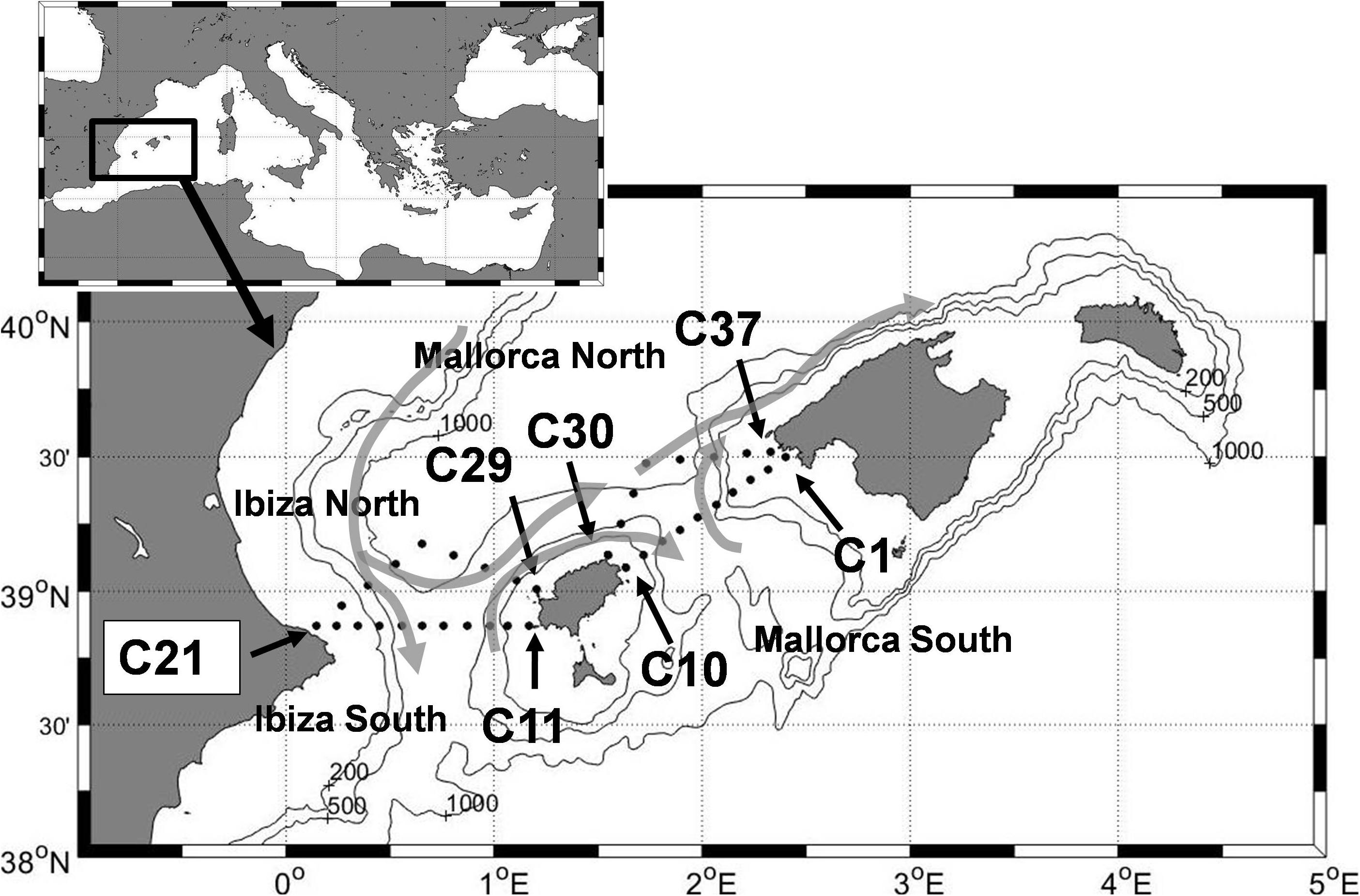
Figure 1. Position of the stations monitored from 1996 to 2019 in the frame of the CANALES, CIRBAL and RADMED projects. These stations are distributed along four sections: Mallorca South (stations C1–C10), Ibiza South (C11–C21), Ibiza North (C21–C29) and Mallorca North (C30–C37). The Mallorca South and North sections form the Mallorca Channel triangle and the Ibiza South and North form the Ibiza Channel triangle. A scheme of the upper layer circulation in the Balearic Sea, inferred from the literature and this study is also included.

The southern part of the WMED cyclonic circuit is formed by the Algerian Current. This current is 30–50 km wide and 200–400 m deep and flows eastwards along the Algerian continental slope (Testor et al., 2005; Pascual et al., 2014). It is unstable, generating cyclonic and anticyclonic eddies. Testor et al. (2005) and Escudier et al. (2016) have shown that anticyclonic eddies have a larger size and longer lifespan than the cyclonic ones. Anticyclonic eddies can reach even the bottom of the Algerian slope and last for 3 years. These eddies follow the pathway of the main current which describes two cyclonic gyres, one of them between 1 and 3.5°E (Western Cyclonic Gyre) and a second one between 4.5 and 8°E (Eastern Cyclonic Gyre, Escudier et al., 2016). Therefore, the eddies detached from the Algerian Current flow eastwards along the Algerian slope and westwards at a latitude of 39° or 40° N. These mesoscale structures can reach the Balearic Channels and constitute a possible means for AW and LIW transport through the Channels.

The Balearic Channels, which are located between the waters flowing through the Algerian basin and those in the Liguro-Provençal area, are consequently considered as a “choke point” for the north-south water, heat and salt exchanges within the WMED (Heslop et al., 2012; Barceló-Llull et al., 2019). A proper and detailed description of the water mass properties and associated transports in the Balearic Channels is of paramount importance for the understanding of the mass, heat and salt budgets in the WMED, as well as the ocean circulation and variability in this basin.

The first attempts to establish the properties of the water masses in the Channels and their associated transports, analyzed a reduced number of oceanographic campaigns, most of them during winter or spring (García-Lafuente et al., 1995; López-Jurado et al., 1995; Pinot and Ganachaud, 1999). These works established that the Northern Current was deflected to the northeast after reaching the Balearic Islands, forming the so-called Balearic Current along the northern slope of the archipelago. Nevertheless, a fraction of the upper and intermediate water masses within this current would flow southwards. The Ibiza Channel was the preferential pathway for the modified AW and WIW flowing within the Northern Current. These authors also found that fresh AW intrusions from the south could occur at the eastern side of the Ibiza Channel and through the Mallorca one, feeding the Balearic Current. This general picture was subject to a high temporal variability and soon it became clear that the hydrographic conditions during any particular campaign could depart strongly from one to other making it necessary the study of long time series covering the complete seasonal cycle. Pinot et al. (2002) was one of the first studies addressing the seasonal variability at the Balearic Channels using a several year time series of observations. This work analyzed 13 surveys from March 1996 to June 1998 and 5 mooring lines in the Ibiza and Mallorca Channels to describe the water mass distributions and transports corresponding to the four seasons of the year.

Additional works have shown that the variability at short time scales could be as large as the variability at seasonal scale and consequently longer time series would be needed (Heslop et al., 2012). These authors analyzed the short time scales by means of a series of 2–3 days glider transects from January to June 2011 in the Ibiza Channel from the SOCIB observing system (Sistema de Observación y predicción Oceánica de las Islas Baleares). Juza et al. (2013) analyzed a similar high resolution data base combined with numerical simulations and Barceló-Llull et al. (2019) studied a series of glider transects in the Mallorca Channel from 2011 to 2018. All these works revealed the high variability of the circulation in the Balearic Channels, both at a seasonal scale, mainly linked to the winter intensification of the Northern Current, and at shorter time scales, associated to mesoscale activity such as eddies at both the northern and southern sides of the Channels.

This study examines the longest time series of CTD seasonal sections in the Balearic Channels from 1996 to 2019. It could be considered as an extension of that by Pinot et al. (2002), who analyzed exactly the same hydrographic stations from 1996 to 1998 in the frame of the CANALES project. The present study uses those data in Pinot et al. (2002), the first extension of CANALES project under the frame of CIRBAL project (1999–2006), and the current Mediterranean monitoring program RADMED operated by the Instituto Español de Oceanografía (IEO) from 2007 to the present. The main objective of this work is to provide a statistical description of the temperature and salinity fields within the Balearic Channels, establishing the seasonal climatologies of hydrographic properties of water masses, their ranges of variability and their mass transports through the Channels.

Data

The Instituto Español de Oceanografía (IEO, Spanish Institute for Oceanography) has monitored the oceanographic conditions in the Balearic Channels since 1996 to the present with a variable periodicity and under the umbrella of different projects. The first one was named CANALES (from the Spanish word for Channels) and lasted from 1996 to 1998. The second project, called CIRBAL (Circulation in the Balearic Channels), collected data from 1999 to 2006. Finally, in the frame of the RADMED project, the Balearic Channels have been monitored from 2007 to the present (López-Jurado et al., 2015; Tel et al., 2016). The first two projects were devoted to the study of the physical properties of the water masses and their circulation within the Balearic Channels (Pinot et al., 2002). The RADMED project is dedicated to the multidisciplinary seasonal monitoring of the continental shelf and slope waters of the Spanish Mediterranean, including the Balearic Islands and some deep stations for the monitoring of the Mediterranean deep waters.

The sampling strategies and the collected variables have changed according to the different projects. Nevertheless, during all the oceanographic campaigns, a CTD vertical profile was collected at all the stations along the four sections within the Balearic Channels (Figure 1). These four sections formed two triangles, one in the Mallorca Channel (from Mallorca to Ibiza Island) and a second one in the Ibiza Channel (from Ibiza to the mainland). The distribution of the stations in triangles was fixed during the first project CANALES, which aimed at having closed boxes for the application of box inverse models (Pinot and Ganachaud, 1999; Pinot et al., 2002). The distance between stations is 5 nautical miles for the straight sections in the southern part of the Channels, and 8 nautical miles for the broken sections at the northern part of the Channels. These distances would be similar to the Rossby radius of deformation in the Balearic Channels, which is around 10 km (Pinot and Ganachaud, 1999; Send et al., 1999).

These four hydrographic sections were sampled during 71 campaigns over 1996–2009. Supplementary Table S1 shows the monitored months and years for every campaign and the project under which each survey was carried out. These CTD data are freely available at standard depth levels in the IBAMar data base¹ and under request in Sea Data Net.

Materials and Methods

This section and the next section (“Results”) are organized following the same structure (sub-sections) to better relate and understand each specific result to the corresponding methodology and objectives. First, the normality of the temperature and salinity distributions is examined, and the mean and median values as well as the dispersion of such distributions are estimated. Secondly, the temperature and salinity covariance functions are defined and the methods used for their estimations are presented. This sub-section aims at obtaining the parameters needed for the application of Optimal Statistical Interpolation. Thirdly, the water masses (AW, WIW, LIW, and WMDW) and the criteria used to define them are described. Finally the methodology corresponding to a box inverse model is presented.

Normality and Measures of Central Tendency and Dispersion

The first objective of this work is to obtain the statistical properties of the temperature and salinity fields in the Balearic Channels, which have a strong variability at seasonal scale. For this reason, all the available campaigns were distributed into four seasonal groups: winter includes surveys from January to March, spring from April to June, summer from July to September, and autumn from October to December. The total number of surveys carried out during each season of the year were: 21 for winter, 24 for spring, 13 for summer and 13 for autumn. Supplementary Figure S1 shows the distributions of the dates for each campaign and the earliest and the latest surveys for each season. As each survey extended along more than 1 day (4 days in general), the date corresponding to each survey is the central one.

Each campaign corresponding to a particular season and year shows different temperature and salinity values because of the natural variability of the sea and the ocean-atmosphere interaction. All the temperature and salinity data corresponding to the same season of the year and the same pressure level are distributed around a certain value. Using the usual terminology in descriptive statistics, such a value is named the central tendency of the distribution (Zar, 2010). This latter, obtained from time series as long as possible, is considered as a climatological value. The mean and the median are usual statistics used to express the central tendency of a distribution. Nevertheless, the most appropriate one depends on the distribution shape. Both values are coincident in the case of a Normal (symmetric) distribution. In case of skewed (asymmetric) distributions, the median is a more appropriate measure of the central tendency. For this reason, Shapiro-Wilk tests were carried out to check the normality of the potential temperature and salinity distributions at the pressure levels 5, 50, 100, 200, 300, 400, 500, and 1000 dbar and for each season of the year (Figure 2).

FIGURE 2

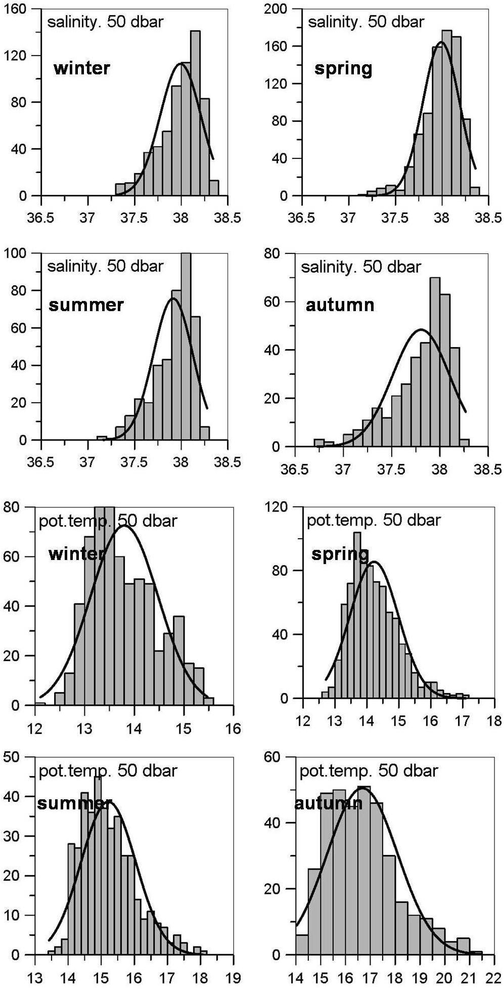
Figure 2. Histograms showing the salinity and potential temperature distribution for the four seasons of the year at the 50 dbar pressure level. A normal distribution was fitted to each distribution (solid line).

Besides the central tendency, the width of the distribution is a fundamental statistic since it provides the range of values that could be expected when a single measurement is obtained. Finally the mean value, the median and the standard deviation were estimated for the potential temperature and salinity for each of the four sections within the Balearic Channels and for each season of the year.

The Covariance Function. Parameters for Optimal Statistical Interpolation

The covariance function of any observed variable informs about the spatial structure of such variable. Besides this, when interpolation is required and the variable is interpolated as a linear combination of the available observations, an optimal linear interpolation can be estimated if the covariance function of the variable and the noise to signal ratio are known (Thiébaux and Pedder, 1987; Pedder, 1993; Gomis et al., 2001; Supplementary Material for mathematical details). In most of the cases, these functions are not known when one single realization of a hydrographic section is available, neither are known the statistical properties of the analyzed variables for the particular region of interest. In practice, the observed variables are decomposed into a background field and a signal on which we are interested plus a noise. The background field is usually modeled as a low order polynomial which should be estimated by generalized least squares, which once again require the knowledge of the covariance function. A possible approach is to estimate the background field by ordinary least squares and then the covariance function from the resulting residuals, and then proceed in an iterative way (Bretherton et al., 1976). Vargas-Yáñez et al. (2005) showed that the periodic repetition of hydrographic sections could be used for the estimation of the covariance function and those parameters needed for the correct use of Optimal Statistical Interpolation.

Let’s consider ϕ_i,t the value of any variable (temperature, salinity, etc.) at the position r_i = (x_i, z_i) within an hydrographic section at time t. Then a background or climatological mean can be estimated for each season of the year as the sampling mean:

$${\widehat{\mathrm{\mu }}}_i=\frac{{\sum }_{t=1}^T{\mathrm{\varphi }}_{i,t}}{T}(1)$$

Being T the times such a location had been sampled for a given season of the year. The hat denotes estimation. The covariance and the correlation functions were estimated for each pair of positions r_i and r_j within the hydrographic section using Eqs (2) and (3):

$$cov({\overline{r}}_i,{\overline{r}}_j)=\frac{{\sum }_{t=1}^T\left({\mathrm{\varphi }}_{i,t}-{\widehat{\mathrm{\mu }}}_i\right)\left({\mathrm{\varphi }}_{j,t}-{\widehat{\mathrm{\mu }}}_j\right)}{T}(2)$$

$$corr({\overline{r}}_i,{\overline{r}}_j)=\frac{{\sum }_{t=1}^T\left({\mathrm{\varphi }}_{i,t}-{\widehat{\mathrm{\mu }}}_i\right)\left({\mathrm{\varphi }}_{j,t}-{\widehat{\mathrm{\mu }}}_j\right)}{\sqrt{{\sum }_{t=1}^T{\left({\mathrm{\varphi }}_{i,t}-{\widehat{\mathrm{\mu }}}_i\right)}^2{\sum }_{t=1}^T{\left({\mathrm{\varphi }}_{j,t}-{\widehat{\mathrm{\mu }}}_i\right)}^2}}(3)$$

The following objective was to find the analytical dependence of the covariance and correlation functions on the coordinates (x_i, z_i) and (x_j, z_j). First, we inspected the dependence of the covariance function on the horizontal coordinates. In this case, the formulas (2) and (3) were evaluated for all pairs of points with the same vertical coordinate z and different values of x. It was assumed that for a fixed depth level, these functions only depended on the horizontal distance Δx. Then, two Gaussian functions were fitted:

$$cov\left(\mathrm{\Delta }x\right)={\mathrm{\sigma }}^2\exp \left[-\frac{\mathrm{\Delta }{x}^2}{2L_x^2}\right](4)$$

$$corr\left(\mathrm{\Delta }x\right)=R_0\exp \left[-\frac{\mathrm{\Delta }{x}^2}{2L_x^2}\right](5)$$

Where σ² and L_x are the parameters obtained from the fit of (4) to the data. σ² is the value of the covariance function for Δx = 0, and represents the variance of the analyzed variable, and L_x is the decaying distance for the covariance function (see also Supplementary Material for details). Analogously, R₀ and L_x are the parameters of the fit for the correlation function.

Notice that the fit for the correlation function assumes a R₀ value for Δx = 0 different from 1. This value accounts for the noise to signal variance ratio:

$$\mathrm{\gamma }=\frac{1}{R_0}-1(6)$$

The parameters σ, L_x, R₀, and γ were estimated for each depth level and consequently could depend on depth.

To find out the dependence of the covariance function on the vertical coordinate, the Eqs (2) and (3) were estimated for all pairs of points with the same x value, but different z_i and z_j values. In this case, it cannot be assumed that the covariance only depends on the vertical distance between observations but also on the specific values of z_i and z_j. The vertical covariance was modeled as:

$$cov(z_1,z_2)={\mathrm{\sigma }}_0\exp [-{\mathrm{\alpha }}_1{(z_1-z_0)}^2-{\mathrm{\alpha }}_2{(z_2-z_0)}^2-\mathrm{\beta }(z_1-z_0)(z_2-z_0)](7)$$

Considering the symmetry of the covariance matrix α₁ = α₂ and making the variable change:

$$z_1=\overline{z}-\frac{\mathrm{\Delta }z}{2}{z}_2=\overline{z}+\frac{\mathrm{\Delta }z}{2}$$

the former equation for the covariance function could be expressed as:

$$cov(z_1,z_2)={\mathrm{\sigma }}_0\exp \left[-\frac{{\left(\overline{z}-z_0\right)}^2}{2L_1^2}\right]\cdot \exp \left[-\frac{\mathrm{\Delta }{z}^2}{2L_2^2}\right](8)$$

Detection of Water Masses and Determination of Their Properties

The water masses which are mainly present in the Balearic Channels, are the Atlantic Water (AW), the Western Intermediate Water (WIW), the Levantine Intermediate Water (LIW), and the Western Mediterranean Deep Water (WMDW). Once the mean and median values had been calculated for each season and hydrographic section, the potential temperature, salinity, potential density and pressure levels corresponding to each water mass were estimated, in order to re-define the climatological properties of the main water masses in the Balearic Channels.

The strongest influence of AW is observed at the sea surface. Therefore, salinity, potential temperature and density for the upper 5 dbar of the water column were averaged for each season and hydrographic section. These values can be considered as indicators of the presence of this water mass at the area of study during the different seasons of the year.

The WIW has been traditionally considered as a cold water mass with potential temperature below 13°C and salinity values ranging between 37.7 and 38.3 (Salat and Font, 1987; López-Jurado et al., 1995). Vargas-Yáñez et al. (2012) considered that the WIW potential temperature and salinity ranges could be even larger and Pinot et al. (2002). Pinot and Ganachaud (1999) used the potential density range 28.8–29.05 to define the layer within the water column occupied by this water mass. Therefore, a first method to identify the properties of the WIW was to select those θS values with potential density values ranging between 28.8 and 29.05 kgm^–3. The minimum θ value within this density range was considered the core of the WIW and the potential temperature, salinity and depth for such minimum were considered as the WIW properties for that oceanographic station and season of the year.

Juza et al. (2019) have shown that the previous methods for the identification of WIW properties have some shortcomings. The use of pre-determined temperature and salinity ranges does not allow to detect and track spatio-temporal changes in water mass properties and may lead to erroneous characterizations and interpretations. For example, an increase of temperature which would be out of ranges would be interpreted as absence or loss of this water mass. To overcome these issues, Juza et al. (2019) have developed a geometry-based approach to detect the presence of WIW and characterize its temperature and salinity properties. This method is based on the WIW definition and the θS diagram shape, taking advantage of the position of the WIW between surface layers and LIW with temperature minima. This method enables to detect properly the WIW properties and their changes at both spatial and temporal scales. Finally, both methods were used for comparison: The minimum potential temperature for the 28.8–29.05 potential density range, and the geometry-based approach.

The core of the LIW was identified as the absolute salinity maximum. Depth, potential temperature and salinity values at the position of such maximum were used to define the properties of this water mass.

Finally, WMDW is the densest water mass within the Balearic Channels. Therefore the maximum potential density was considered as the core of this water mass. In some shallow stations, the deepest levels were occupied by a mixing of LIW and WMDW and it would not be appropriate to consider these waters as WMDW. First it was considered the possibility of following Pinot and Ganachaud (1999) and identifying WMDW as the densest waters for each station with a potential density higher than 29.1 kg/m³. Nevertheless, the analysis of the mean and median θS diagrams (see “Results” section) showed that this density value was very close to the LIW core and waters with this density would be a mixing between LIW and WMDW with a higher percentage of the former water mass. Finally, the used criterion was to identify the properties of WMDW at each station as those corresponding to the maximum potential density if that value was higher than 29.11 kg/m³. Notice that the depth of this maximum is not always the maximum depth of the station. In such cases, it simply indicates that the maximum density is reached somewhere above the bottom depth and that the potential density remained constant to the sea bottom. Also notice that for each campaign the maximum density reached at each station will be different depending on the recent history of deep convection and modification of WMDW (see for instance Schroeder et al., 2010). As a result, WMDW temperature and salinity values will also be different for each campaign. In this work, the mean and median values from the whole time series will be analyzed.

Circulation and Transports Associated to the Average θS Distributions. Application of a Box Inverse Model

Once the average distributions of potential temperature and salinity had been obtained, the circulation and the water mass transports associated to such distributions were estimated. Considering that the climatological θS values are very close to the most likely values found in the Balearic Channels, the associated currents and circulation would also describe the most likely circulation patterns in this area of the WMED.

The box inverse problem method was developed by Wunsch (1978, 1996) and was used to determine the circulation in the Balearic Sea and the Balearic Channels by Pinot and Ganachaud (1999) and Pinot et al. (2002). In summary, this method assumes the conservation of certain properties through a closed box. The model used at the present work follows Pinot and Ganachaud (1999) and Pinot et al. (2002) and assumes the mass conservation for four layers defined from the sea surface to the 28.8 isopycnal, from 28.8 to 29.05, from 29.05 to 29.1, and finally from the 29.1 isopycnal to the sea bottom. In addition to the mass conservation for these four layers, a fifth equation was obtained for the mass conservation for the whole water column. An error term was included for the transport at each layer (see Supplementary Material for mathematical details). Following Pinot and Ganachaud (1999) and Pinot et al. (2002), Ekman transport and diapycnal mixing was not taken into account in the conservation equations and these processes were considered as included in the error term (Wunsch, 1978, 1996; Pinot and Ganachaud, 1999; Pinot et al., 2002). This inverse box model has been extensively applied in different oceanographic regions. Thus, Hernández-Guerra and Talley (2016) and Hernández-Guerra et al. (2019) estimated the Meridonal Overturning Circulation in the Indian-Pacific and Atlantic Oceans, respectively, and Hernández-Guerra et al. (2017) and Casanova-Masjoan et al. (2018) in the western and eastern boundaries of the North Atlantic Subtropical Gyre.

Results

Normality and Measures of Central Tendency and Dispersion

The potential temperature and salinity values were assorted according to their season of the year and pressure level. Figure 2 illustrates the case for the 50 dbar level, but the same analysis was performed at 5, 50, 100, 200, 300, 400, 500, and 1000 dbar. Figure 2 shows that the potential temperature and salinity distributions are not symmetric. Almost in all the cases, the null hypothesis (normality of the distribution) was rejected by the Shaphiro-Wilk tests. In addition, Smirnov-Kolmogorov tests produced the same results.

Hence, the median values were chosen to describe the climatological properties of water masses. Figures 3A,B show the median vertical salinity and potential temperature profiles for the four seasons of the year and averaged for the whole area (four sections). Figures 3C,D show a zoom of the upper 100 dbar of the water column. The upper 100 dbar of the water column show the presence of a seasonal thermocline which develops from spring to summer and then starts to be eroded in autumn. This is superimposed on a permanent thermocline associated to the mixing of the AW with the intermediate water masses (WIW and LIW) which flow below. During the winter, only the permanent thermocline (much smoother than the seasonal one) can be observed. A strong halocline is also observed. The surface salinity values also show some seasonality with minimum values during summer, and maximum values in winter. These fluctuations are weaker than the temperature ones and the halocline is dominated by the permanent one. The seasonal and geographic variability of the surface salinity and temperature can be checked in Tables 1.1, 1.2, 1.3, 1.4. These tables also indicate the hydrographic properties of the WIW, LIW and WMDW.

FIGURE 3

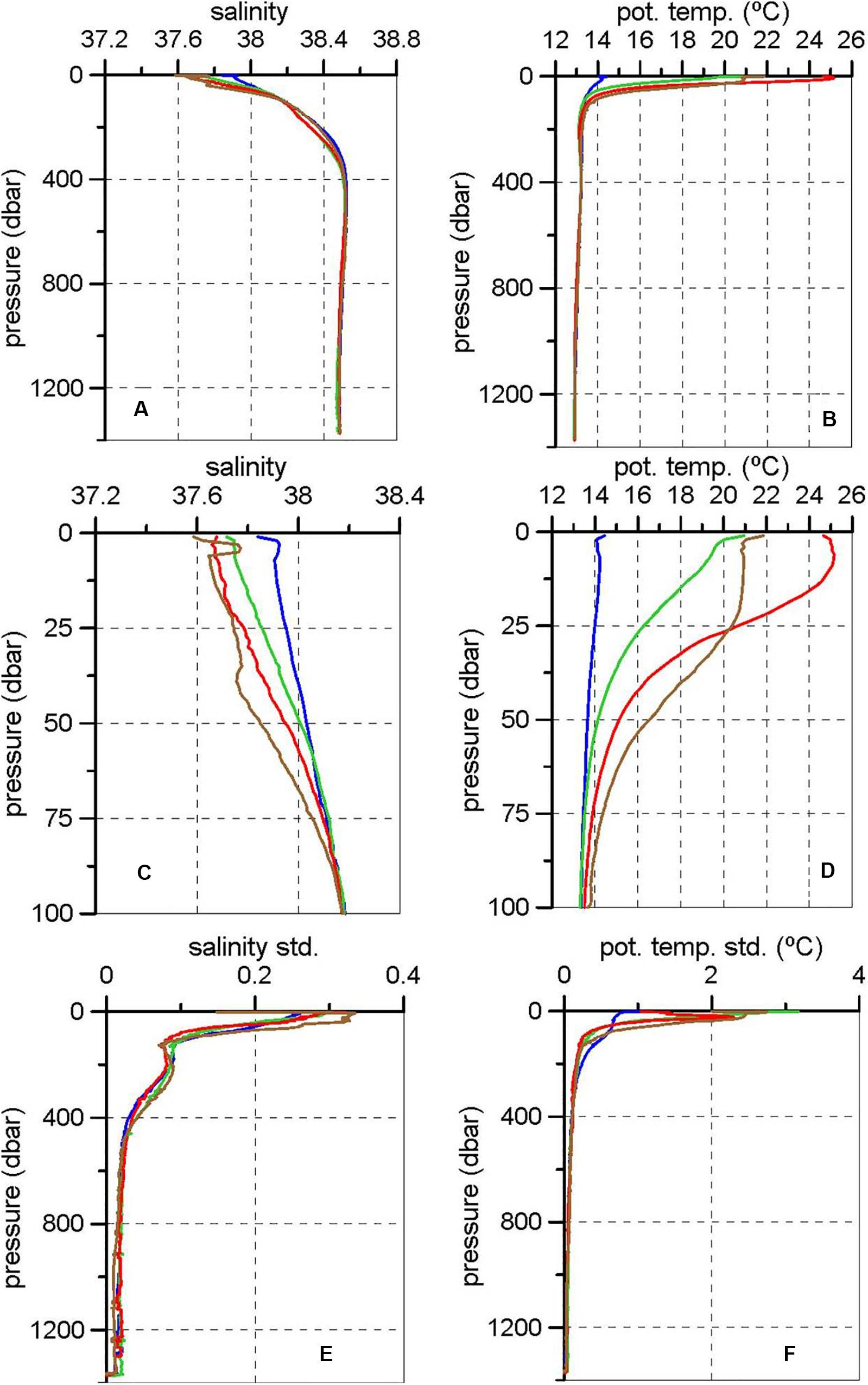
Figure 3. Median vertical profiles of salinity (A) and potential temperature (B) for each season of the year for the four hydrographic sections, and respective zooms in the upper 100 dbar (C,D). Vertical profiles for the salinity and potential temperature standard deviation (E,F, resp.). Seasons are indicated in color: winter (blue), spring (green), summer (red), and autumn (brown).

TABLE 1

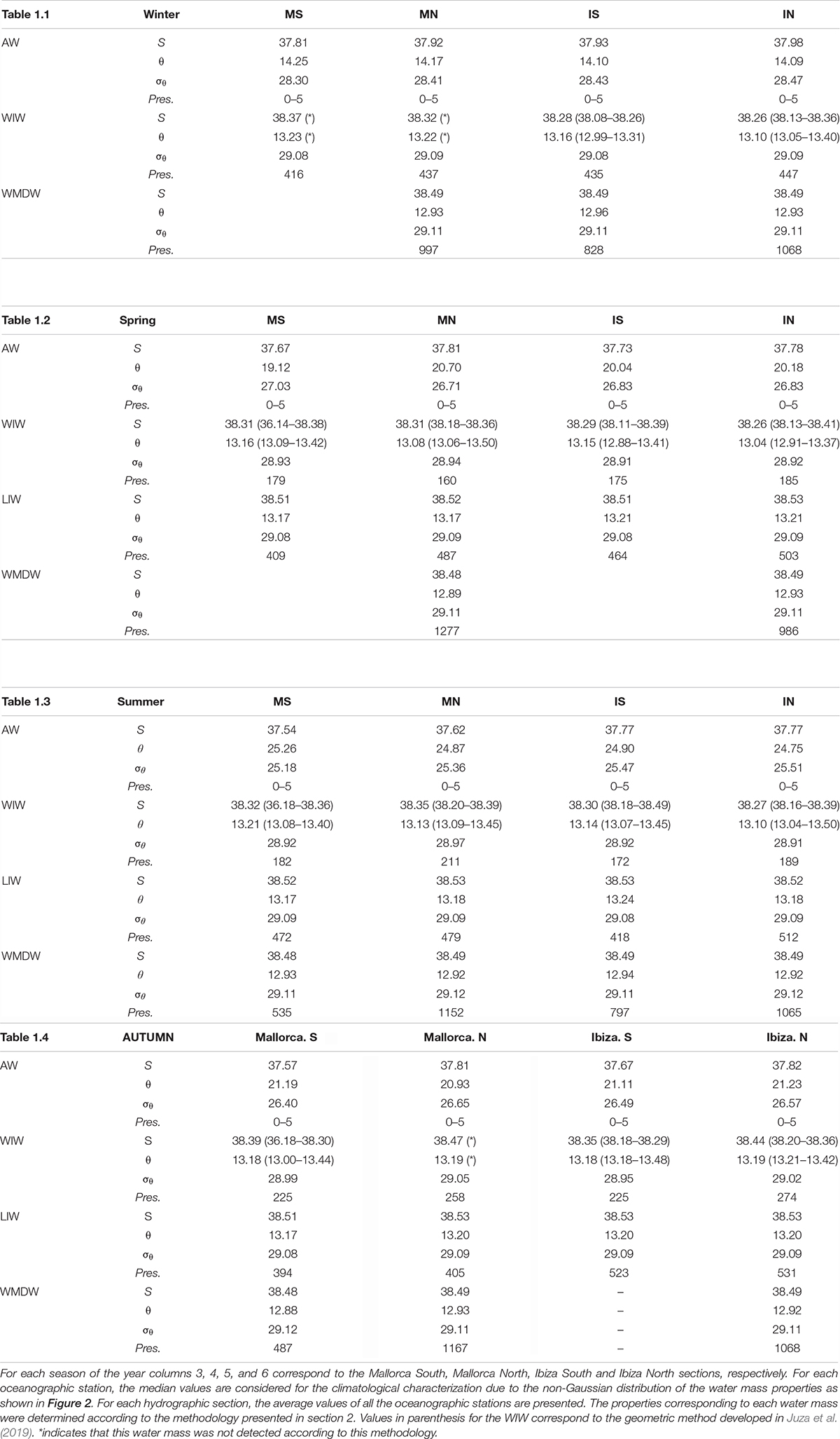
Table 1. Tables 1.1, 1.2, 1.3, and 1.4 show the climatological properties of AW, WIW, LIW, and WMDW for winter, spring, summer and autumn.

Figures 3E,F show the seasonal variability of the standard deviation profiles. Both salinity and potential temperature standard deviations decrease sharply with depth. In the case of salinity, the surface standard deviation has not a strong seasonality and values vary between 0.2 and 0.3 during the whole year. The surface temperature standard deviation is minimum in winter (1°C) and increases from spring with values above 2°C. Although salinity and temperature distributions depart from normality, it can be accepted that values up to 1.96 standard deviations above and below the median values are likely to be observed (Zar, 2010). Therefore, winter θS values below 13°C and above 38.1 at surface are not exceptional. Similarly, summer values above 27°C and below 37.5 cannot be considered as anomalous ones. Both salinity and temperature standard deviations decrease abruptly for the upper 100 dbar following a Gaussian function. Nevertheless, this behavior is interrupted in the case of salinity by a relative maximum centred around 200 dbar and then continues decreasing linearly to a value close to 0.04 at 400 dbar and finally keeps constant to the sea bottom. In the case of temperature, the standard deviation decreases almost linearly from 100 dbar (0.5°C) to the 400 dbar level (0.06°C) and then remains constant to the sea bottom. The standard deviation does not show a clear seasonality below the 100 dbar level.

The Covariance Function. Parameters for Optimal Statistical Interpolation

Figures 4A (winter), C (spring), E (summer), and G (autumn) show the salinity covariance as a function of the horizontal distance (Δx) at three selected depth levels (25, 50, and 100 m) for the four seasons of the year. This analysis was also performed for all vertical levels from the sea surface to the bottom and for the potential temperature. In order to estimate the analytical form of the salinity and potential temperature covariance, a Gaussian function was fitted for each depth level (see data and methods section and the insert at the left top of Figure 4). The variance, which is estimated from this fit, shows a clear dependence on depth as shown in Figures 4B (winter), D (spring), F (summer), and H (autumn). The variance seems to decrease as a normal function from the sea surface to 100 m approximately, then it decreases linearly until 400 m, and finally remains quasi-constant from 400 m to the sea bottom. On the contrary, the horizontal decaying distance does not show any clear depth dependence and it is finally considered as the mean value along the water column. The same behavior is observed for the noise/signal ratio and the mean value along the water column was chosen as a constant value not dependent on depth. To clarify these ideas, the horizontal covariance for the winter salinity at the upper 100 m, could be expressed as:

FIGURE 4

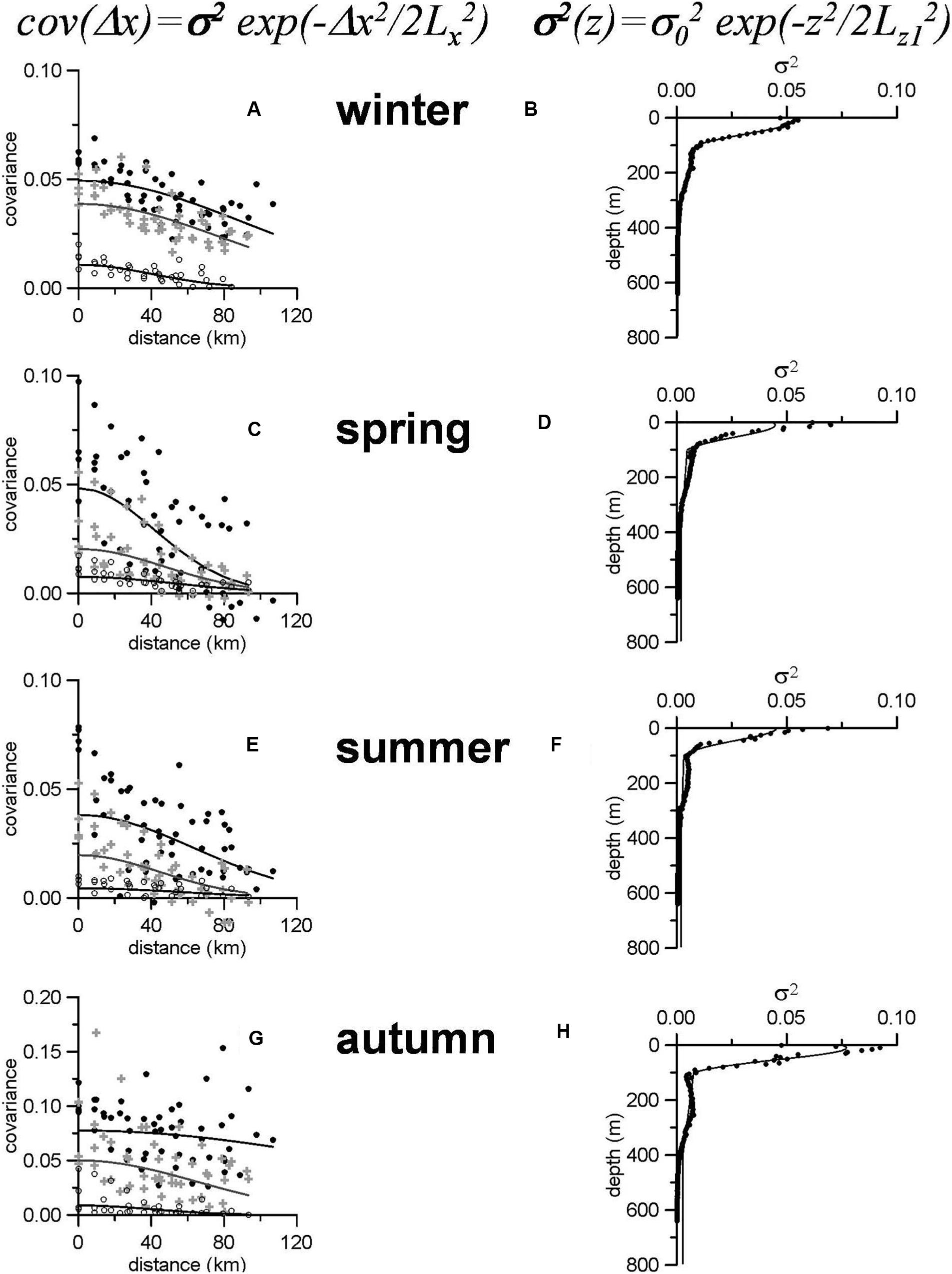
Figure 4. (A, winter), (C, spring), (E, summer), and (G, autumn) are the salinity covariance as a function of the horizontal distance in km for the 25 (black dots), 50 (gray crosses) and 100 m (open circles) depths for the four seasons of the year. Solid lines are a Gaussian fit according to the formula on the left at the top of the panels. σ² is the variance for each depth level. (B, winter), (D, spring), (F, summer), and (H, autumn) show the depth dependence of the σ² value estimated for each depth level. This depth dependence for the upper 100 m is modeled by means of the formula on the right at the top of the panels. Then a linear decrease of the variance is assumed from 100 to 400 m, and a constant value below this depth level.

$$cov(\mathrm{\Delta }x,z)={\mathrm{\sigma }}_0^2\exp \left[-\frac{{\left(z-z_0\right)}^2}{2\cdot L_{z,1}^2}\right]\exp \left[-\frac{\mathrm{\Delta }{x}^2}{2\cdot L_x^2}\right]=0.054\exp \left[-\frac{{\left(z-10\right)}^2}{2\cdot {48}^2}\right]\exp \left[-\frac{\mathrm{\Delta }{x}^2}{2\cdot {50}^2}\right](9)$$

The z₀ in the above formula accounts for the fact that the maximum variance is not always at the sea surface. All the parameters involved in the previous formula corresponding to the four seasons of the year and for both the salinity and potential temperature are presented in Table 2. The two first factors in (9) express the dependence of the variance on the depth level. It should not be confused with the decrease of the covariance with the vertical distance between pairs of points.

TABLE 2

Table 2. Parameters for the analytical expressions for the covariance function for salinity and potential temperature in the Balearic Channels (see Eq. 11).

Figure 5 shows the salinity covariance estimated for each pair of values z₁ and z₂ using (2) for some selected stations within the Mallorca South section and for the four seasons of the year. Constant covariance isolines take the form of ellipses and the covariance decreases as the semi-axis increases justifying the use of (7) and (8) to model the analytical form of this function. Nevertheless, this behavior was only observed for the upper 100 m of the water column.

FIGURE 5

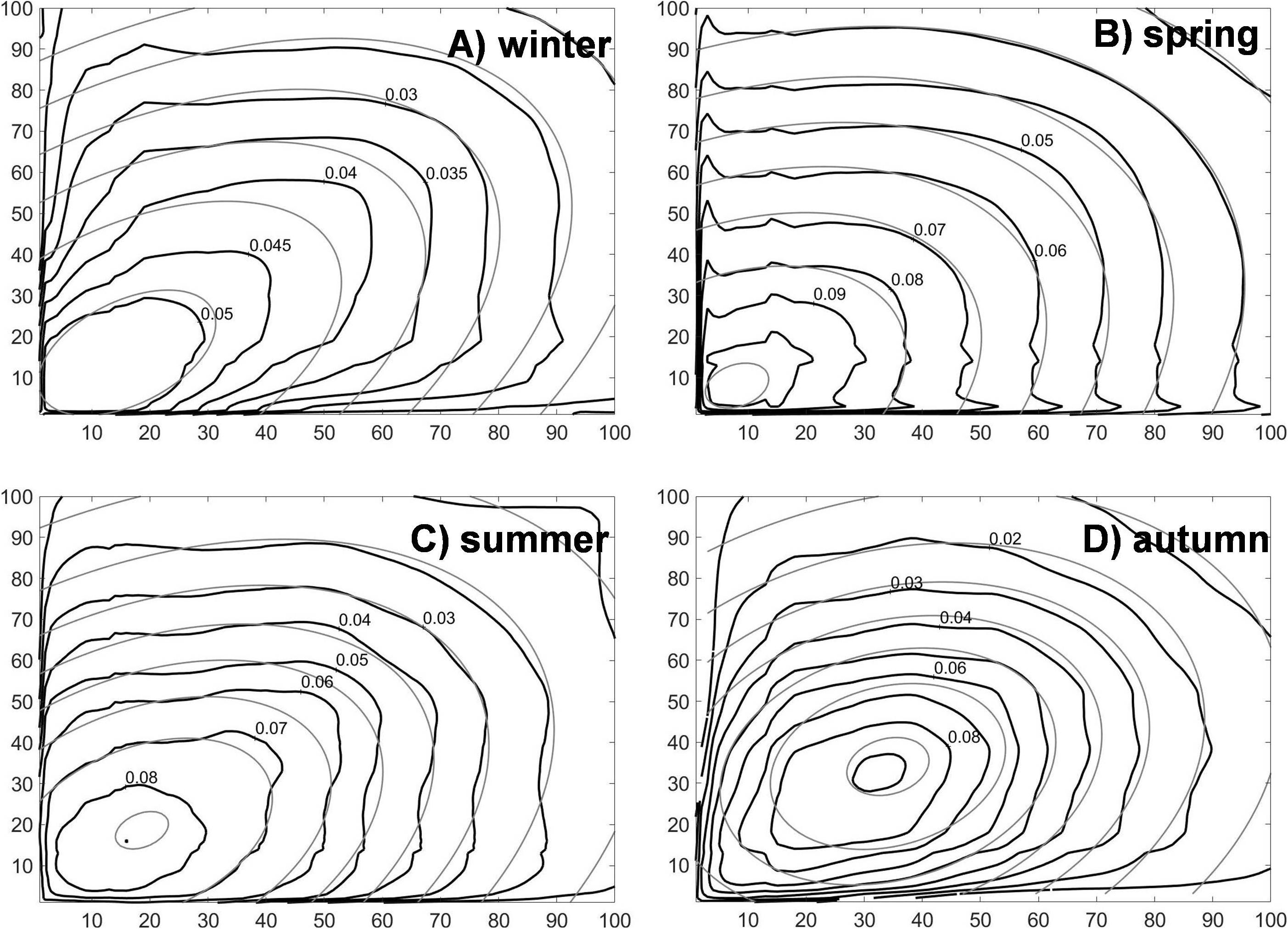
Figure 5. Black lines indicate the salinity covariance estimated for pairs of points at fixed horizontal positions and depth levels z1 and z2 (horizontal axis). The gray lines are the least square fit using equations (7) and (8). (A) is for winter, (B) for spring, (C) for summer, and (D) for autumn.

Once again to clarify these results, equation (10) shows the result of the fit for the salinity winter covariance at the upper 100 m:

$$cov(z_1,z_2)={\mathrm{\sigma }}_0^2\exp \left[-\frac{{\left(\overline{z}-z_0\right)}^2}{2L_{z,1}^2}\right]\exp \left[-\frac{\mathrm{\Delta }{z}^2}{2L_{z,2}^2}\right]=0.062\exp \left[-\frac{{\left(\overline{z}-11\right)}^2}{2\cdot {45}^2}\right]\exp \left[-\frac{\mathrm{\Delta }{z}^2}{2\cdot {53}^2}\right](10)$$

Notice that the first two factors in (10) explain the depth dependence of the variance. The only difference with (9) is that in that case there was one single depth level, while in the present case the variance decreases with the average value of both depth levels. It was checked for all the seasons of the year and for both the salinity and potential temperature that the depth dependence obtained from the analysis on the vertical direction (Eqs 7, 8, and 10) and that inferred from the analysis on the horizontal coordinate were consistent. The third factor in (10) accounts for the vertical decay of the covariance with the vertical distance between pairs of points. The combination of the results obtained from the analysis on fixed depth levels (dependence on the horizontal distance) and the analysis for fixed horizontal positions (dependence on the vertical distance) allowed us to propose the following analytical form for the covariance function:

$$cov(z_1,z_2\mathrm{\Delta }x)={\mathrm{\sigma }}_0^2\exp \left[-\frac{{\left(\overline{z}-z_0\right)}^2}{2L_{z,1}^2}\right]\exp \left[-\frac{\mathrm{\Delta }{z}^2}{2\cdot L_{z,2}^2}\right]\exp \left[-\frac{\mathrm{\Delta }{x}^2}{2\cdot L_x^2}\right]0\le z\le 100m(11a)$$

$$cov(z_1,z_2,\mathrm{\Delta }x)=\left[a-b(\overline{z}-100)\right]\exp \left[-\frac{\mathrm{\Delta }{z}^2}{2\cdot L_{z,2}^2}\right]\exp \left[-\frac{\mathrm{\Delta }{x}^2}{2\cdot L_x^2}\right]100\le z\le 400m(11b)$$

$$cov(z_1,z_2,\mathrm{\Delta }x)=c\exp \left[-\frac{\mathrm{\Delta }{z}^2}{2\cdot L_{z,2}^2}\right]\exp \left[-\frac{\mathrm{\Delta }{x}^2}{2\cdot L_x^2}\right]z\ge 400m(11c)$$

L_x (the horizontal decaying distance of the covariance function) and $\text{γ=}\raisebox{1ex}{${\sigma }_{\text{ε}}^2$}\!\left/ \!\raisebox{-1ex}{${\sigma }^2$}\right.$ (the noise to signal ratio) were considered constant along the water column and a, c in (11b) and (11c) were chosen in such a way that the covariance was a continuous function.

Detection of Water Masses and Determination of Their Properties

Figures 6–9 show the θS diagrams for the four hydrographic sections (Mallorca South, Mallorca North, Ibiza South and Ibiza North, respectively) and for the four seasons of the year. Gray (black) dots correspond to the median (mean) values at each oceanographic station and depth level for each hydrographic section. The upper 100 dbar have not been considered in order to better highlight the properties of intermediate and deep waters.

FIGURE 6

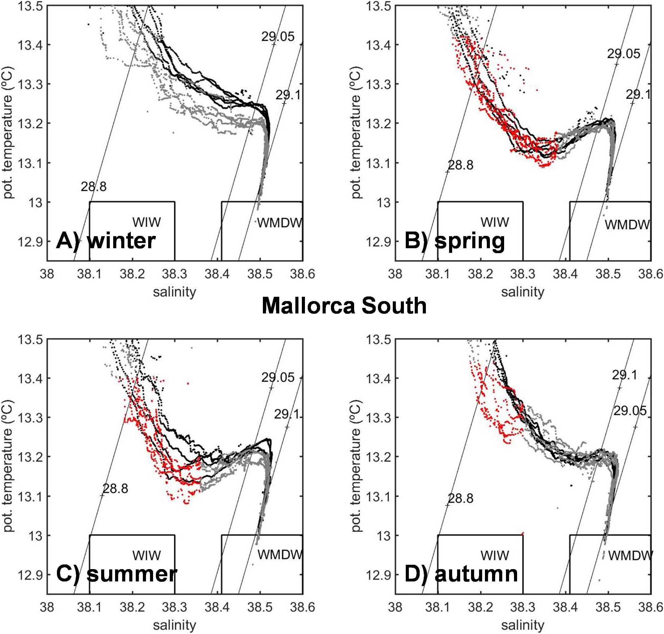
Figure 6. θS diagrams for the Mallorca South section in winter (A), spring (B), summer (C), and autumn (D). The upper 100 dbar have been removed to focus on the characteristics of intermediate and deep waters. σ_θ contours for sigma-theta values 28.8, 29.05, and 29.1 have been included to show the layers corresponding to the WIW (28.8–29.05), LIW (29.05–29.1), and WMDW (> 29.1) according to Pinot and Ganachaud (1999) and Pinot et al. (2002) criterion. Gray dots are median values, black dots are mean values and red dots are those values corresponding to WIW as detected by the geometry-based method in Juza et al. (2019). Median and mean values have been calculated for each oceanographic station and depth level within each hydrographic section. Two boxes indicating the θS ranges for WIW (according to López-Jurado et al., 1995) and the ranges for the WMDW (Pinot et al., 2002) have been included.

FIGURE 7

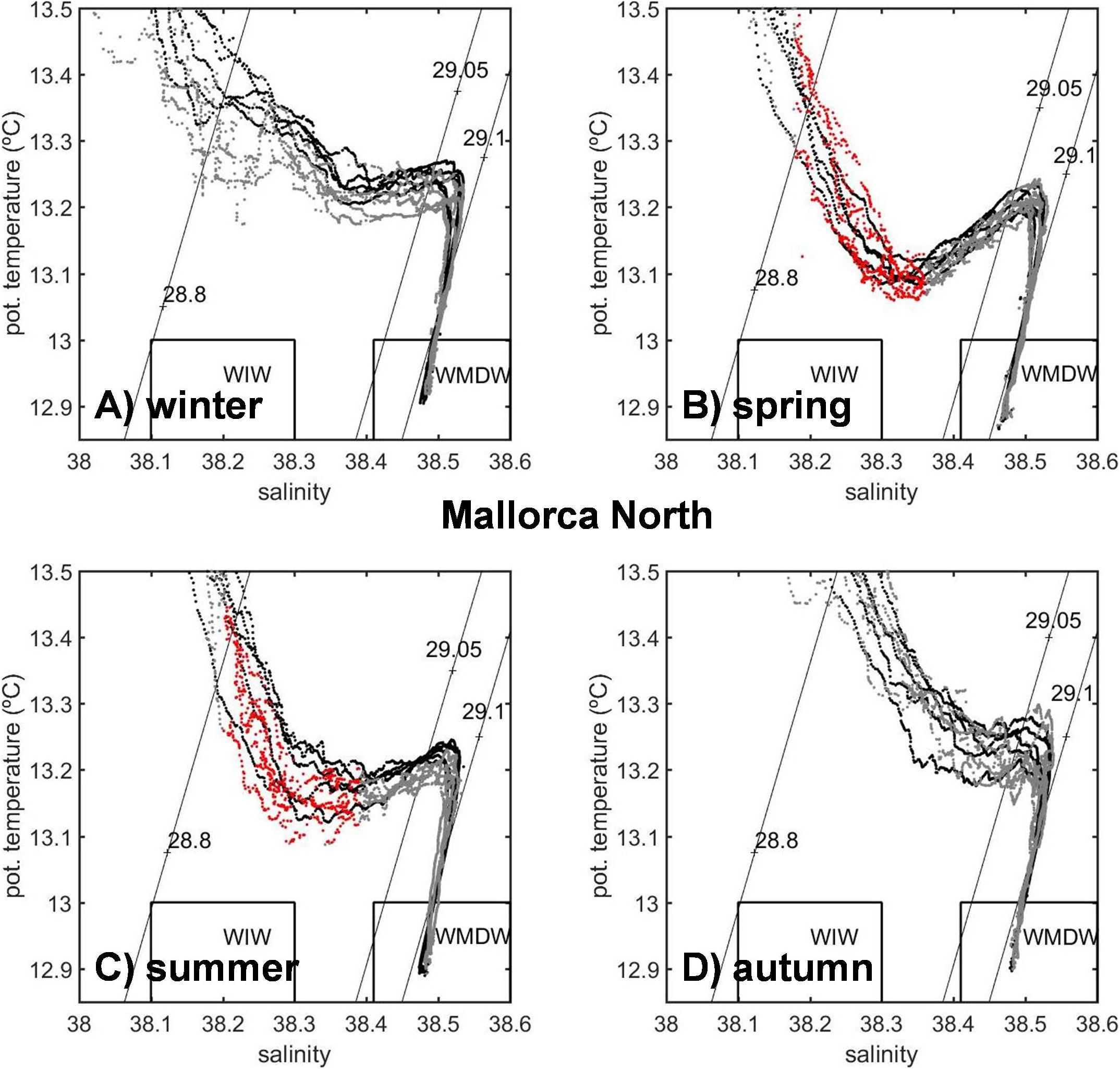
Figure 7. Same as Figure 6 for the Mallorca North section. Winter (A), Spring (B), Summer (C), Autumn (D).

FIGURE 8

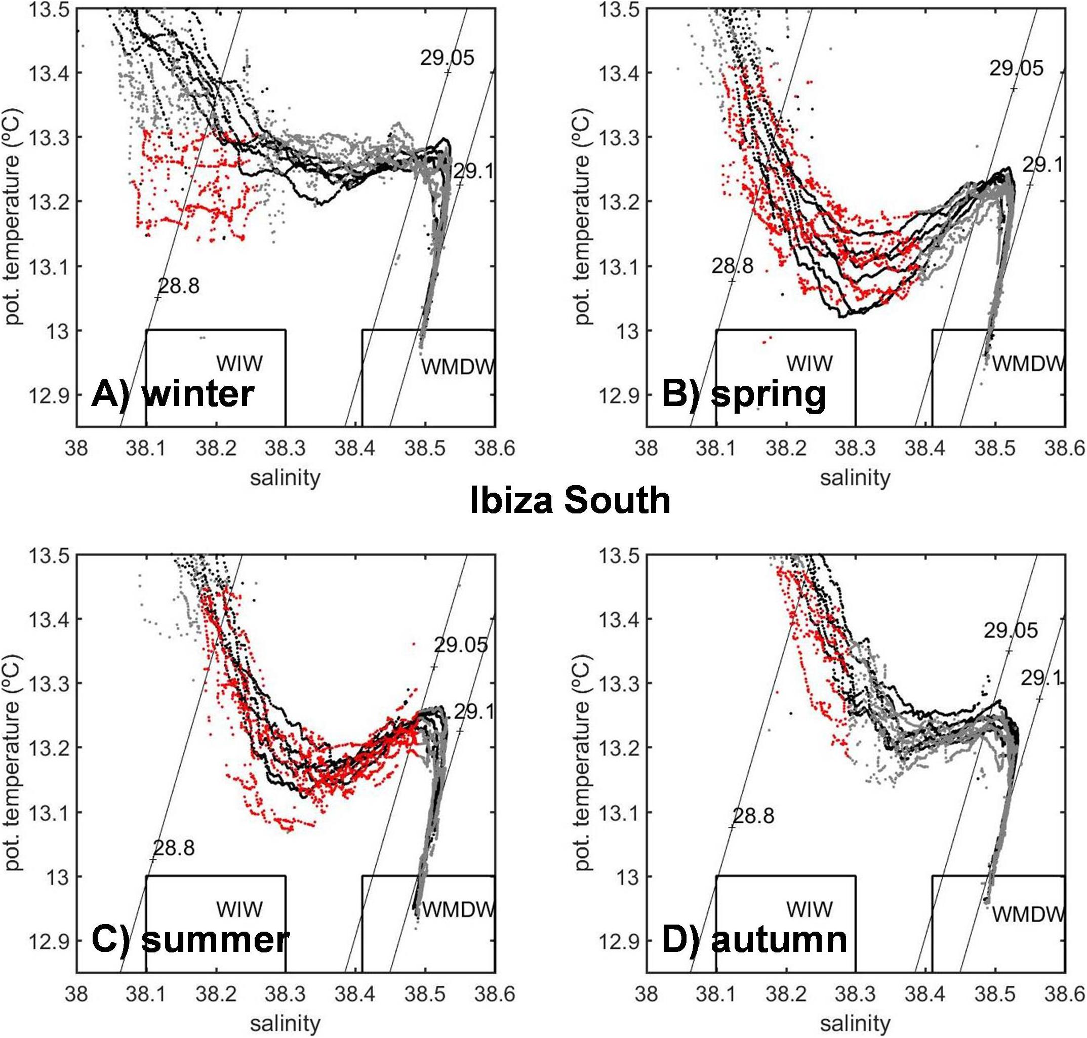
Figure 8. Same as Figure 6 for the Ibiza South section. Winter (A), Spring (B), Summer (C), Autumn (D).

FIGURE 9

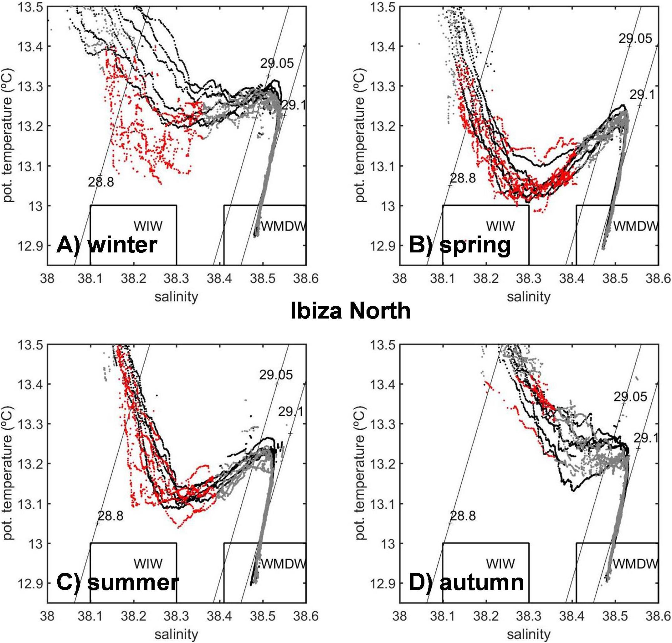
Figure 9. Same as Figure 7 for the Ibiza North section. Winter (A), Spring (B), Summer (C), Autumn (D).

The θS diagrams based on the median climatological values in the Mallorca South and North sections (Figures 6, 7) show lower potential temperature values than those based on mean values for the winter and summer seasons in the density range 28.8–29.05 which are the values considered for the WIW by Pinot and Ganachaud (1999) and Pinot et al. (2002). The same is observed for winter, summer and autumn at the Ibiza South section (Figure 8) and for winter and summer at Ibiza North (Figure 9). Some of the median values lie within the traditional temperature and salinity ranges which define the WIW at Ibiza South in winter and spring (Figures 8A,B) and at Ibiza North during spring (Figure 9B). Additionally, besides the considerable smoothing of the median and mean θS diagrams, they show properties close to the usually accepted values for WIW during spring at Ibiza North and during winter only with the median values. This water mass corresponds to the potential density range 28.8–29.05 kg/m³ as previously considered and its depth range oscillates between 140 and 274 m.

As previously mentioned, the θS values found for the Ibiza Channel during winter and spring are close to the WIW traditional range, with some values entering within such range. Nevertheless, the classical definition of WIW, which is based on a fixed-range criterion (with potential temperature below 13°C and salinity between 37.7 and 38.3) would fail to detect this water mass in almost all the cases if the smoothed climatological values were used. On the contrary, the geometry-based method allows to identify as WIW θS values above the 13°C threshold. Those values have been displayed in red in Figures 6–9. For each season of the year and each hydrographic section, the θS range corresponding to the WIW is evaluated according to the geometric criterion. These intervals are also provided in parenthesis in Table 1.

The LIW also occupies the density range already considered in previous works (29.05–29.1). The salinity values at the core of this water mass are relatively constant throughout the year, ranging from 38.51 to 38.53. Its depth range is 394–531 m. Its potential temperature varies between 13.17 and 13.23° C. Finally, the WMDW was not always detected during all the seasons of the year and all the sections according to the specified criterion (potential density larger than 29.11 kg/m³). The maximum density values reached 29.12 kg/m³. The WMDW salinity values oscillate between 38.48 and 38.49 and the potential temperature values between 12.88 and 12.92°C (Table 1).

Circulation and Transports Associated to the Average θS Distributions. Application of a Box Inverse Model

The current velocity at the reference level (sea bottom) is estimated using the mass conservation for four layers defined by the potential density values: surface/28.8/29.05/29.1/bottom. Figure 10 shows the absolute geostrophic velocity at the Ibiza South section (the corresponding salinity section is presented in Supplementary Figure S10). The same results for the Mallorca South section are presented in Figure 11 and Supplementary Figure S11. All the sections have been divided into an upper layer, which has been considered as the upper 300 m, and a lower layer extending from 300 dbar to the sea bottom. According to Table 1, the WIW depth range rarely exceeds 300 dbar, while LIW is mainly observed between 400 and 500 dbar. Therefore, it was considered that the upper 300 dbar could be useful for describing the AW and WIW properties, while LIW and WMDW would correspond to the layer below. In order to enhance the gradients observed at the upper layer, the height of both parts of the vertical sections do not keep proportionality with their depth interval.

FIGURE 10

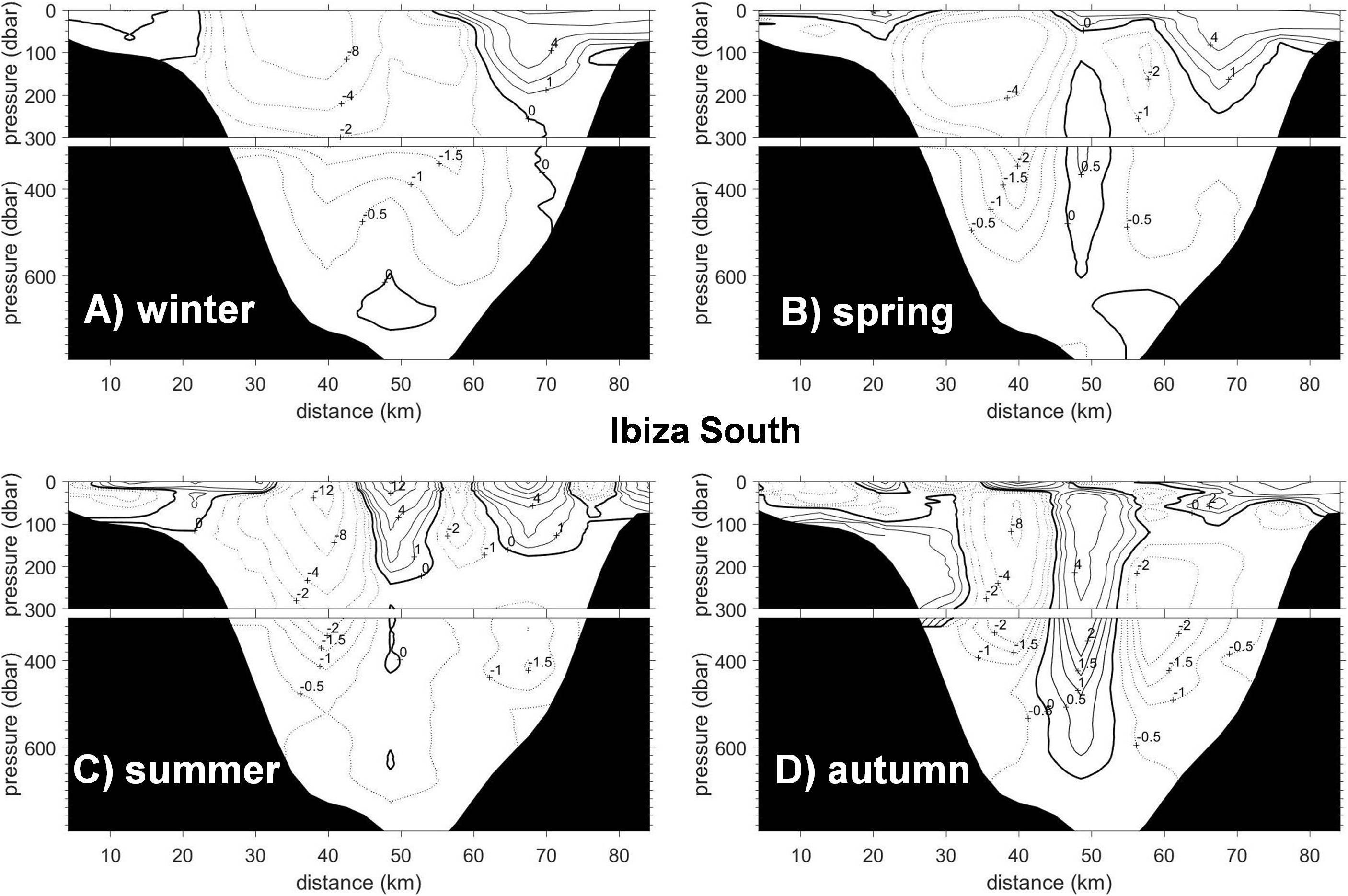
Figure 10. Cross section absolute geostrophic velocity (in cm/s) at the Ibiza South section for winter (A), spring (B), summer (C), and autumn (D). Solid lines correspond to positive velocities which are directed to the North (into the paper), while negative velocities are represented by dashed lines and are directed to the South (out of the paper). The velocity contour intervals for the upper 300 dbar are 0, 1, 2 4, 8, 12, 16, and 20 cm/s (both positive and negative). The contour interval for the velocity from 300 dbar to the sea bottom are 0, 0.5, 1, 1.5 and 2 cm/s (both positive and negative).

FIGURE 11

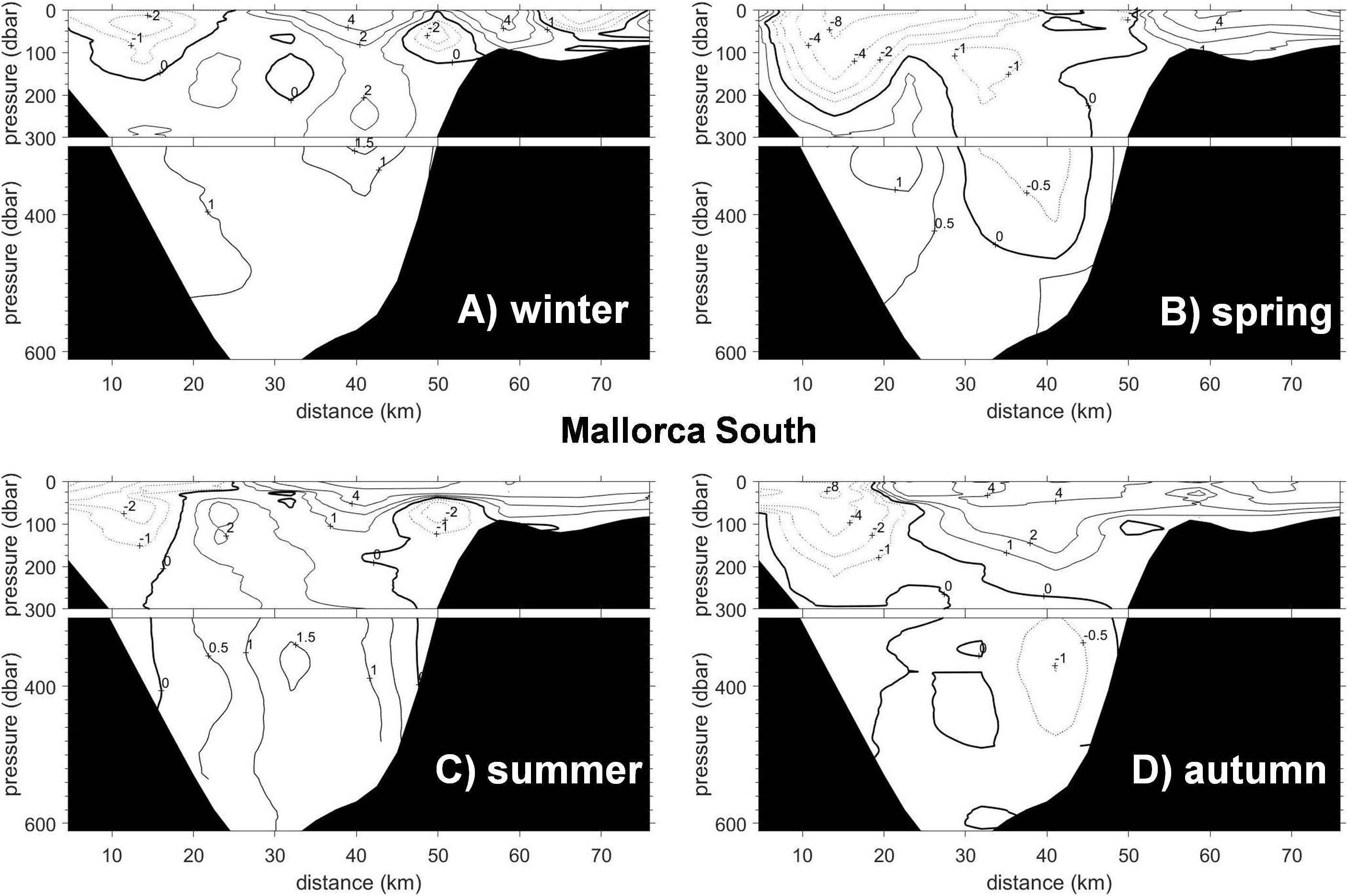
Figure 11. Same as figure for the Mallorca South section. Winter (A), Spring (B), Summer (C), Autumn (D).

Table 3 indicates the mass transports in 10⁹ kg/s (approximately 1Sv) for the upper and the lower layers, for the four sections and the four seasons of the year. The upper layer is considered as the sum of the two upper layers used in the inverse model, that is, from the surface to the 28.8 kg/m³ surface, and from the 28.8 to the 29.05 kg/m³ surface. The lower layer is the sum of the two lower layers in the model, from 29.05 to 29.1 and from 29.1 to the bottom.

TABLE 3

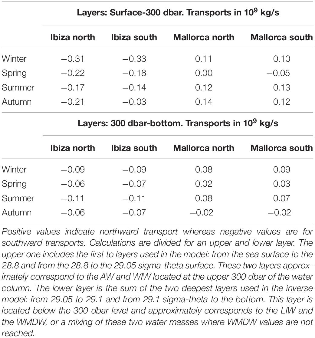
Table 3. Transports in 10⁹ kg/s for the four sections analyzed in this work.

In the Ibiza Channel, the water mass transports are southwards in both layers and along the whole year, while in the Mallorca Channel, they are generally directed northwards, except at the upper layer of Mallorca South in spring, and at the deep layer of both Mallorca sections in autumn. Such transports are also higher in the Ibiza than in the Mallorca Channels. These results are in agreement with previous studies (Pinot et al., 2002; Heslop et al., 2012; Juza et al., 2013).

Figure 10 also shows that the flow has more spatial variability in the upper 300 dbar where different directions alternate, whereas it is more uniform in the lower layer. Considering the mass transports calculated between each pair of hydrographic stations (Supplementary Tables S2A–D), a schematic circulation for the upper layer in the Balearic Channels is proposed in Figures 12A–D. In the lower layer, the circulation pattern is more homogenous, hence only the net mass transports are presented in Table 3.

FIGURE 12

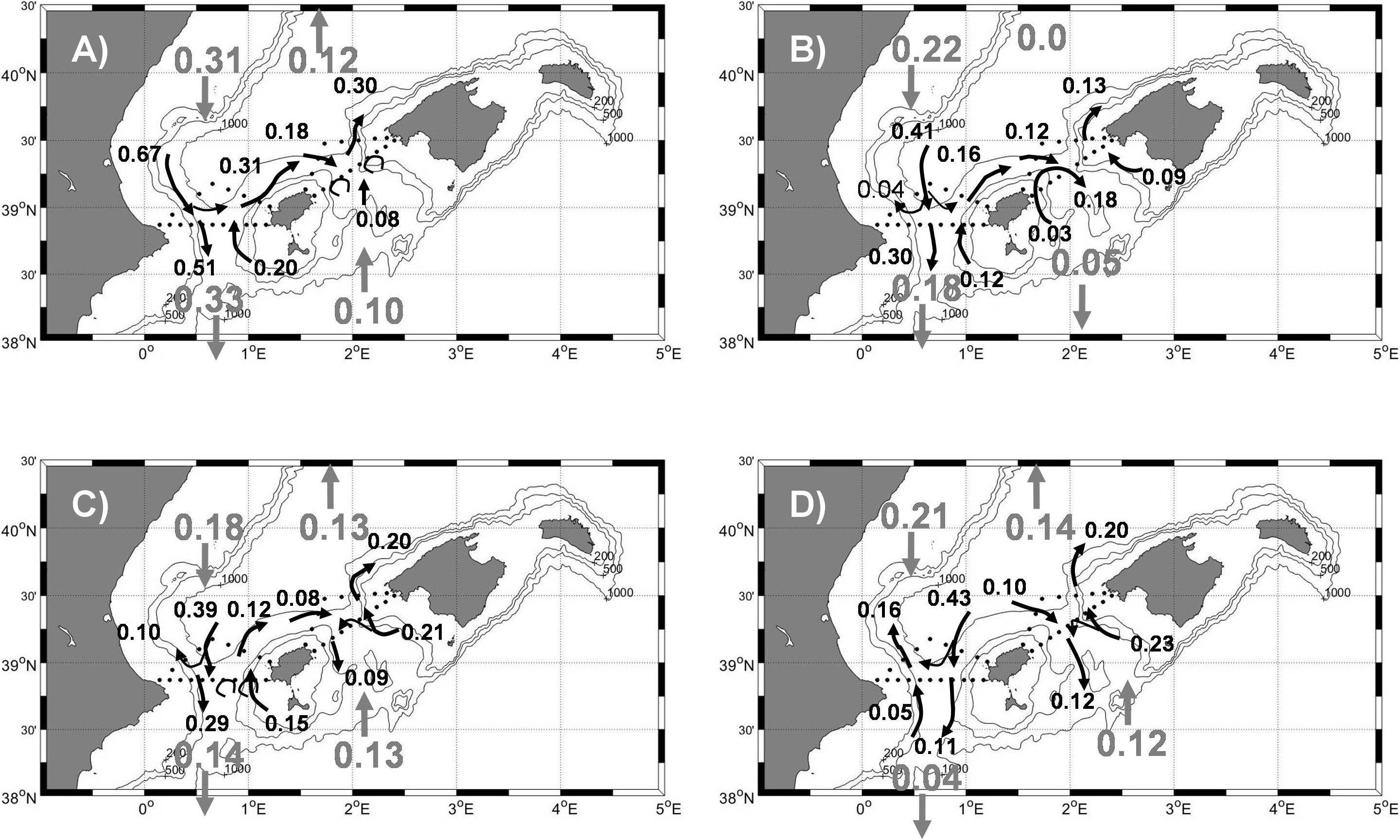
Figure 12. Schematic circulation in the upper layer (AW + WIW) during winter (A), spring (B), summer (C) and autumn (D). Mass transports are expressed in 10⁹ kg/s, which approximately correspond to 1 Sverdrup. Net transports for the upper layer are expressed with gray numbers.

Discussion

The mean values of any property, calculated from a long time series of data at different depth levels, are generally used to define the climatological values of such property. In the case of the hydrographic conditions in the Balearic Channels, we have shown that median values are more appropriate statistical estimates than mean values. As shown in Figure 2, the salinity and potential temperature distributions are not symmetric, and the normality of these distributions was rejected by means of Shapiro-Wilk tests. While the salinity distributions in the upper layers (Figures 2A–D) show an asymmetric tale at low salinity values, the potential temperature distribution shows a tale for high values (Figures 2E–H). These features would indicate the irruptions of AW eddies or filaments detaching from the Algerian Current and moving northwards through the Balearic Channels. Another argument in favor of the use of median values arises from the analysis of θS diagrams and the identification of the different water masses present in the Balearic Sea. Using both mean and median values, the vertical θ and S profiles or θS diagrams are much smoother than those obtained for one single survey. However, the degree of smoothing associated to the mean values seems to be too high and prevent from identifying the presence of some water masses within the Balearic Channels. In particular, using mean values, the θS diagram associated with the winter conditions in the Mallorca South section (Figure 6A) would show an almost linear mixing between AW and LIW flowing below. On the contrary, a relative temperature minimum, suggesting the presence of WIW, could be appreciated considering the median values (Figure 6A). During the summer and autumn, the potential temperature in the 28.8–29.05 kg/m³ potential density range is lower with the median values than with the mean values (Ibiza South, Figures 8C,D). Moreover, some of the median values lie within the traditional ranges defined for WIW (Figures 8A,B, 9B). On the contrary, no mean value corresponds to such ranges in any of the cases analyzed in this study. Therefore, the use of the median shows more clearly the presence and the influence of WIW in the Balearic Channels.

Another interesting feature arising from the analysis of the climatological values in the Balearic Channels is the existence of a clear seasonal cycle, not only for temperature, but also for salinity in the upper layer. The winter median temperature of the surface layer ranges between 14.09 and 14.25°C and the surface salinity ranges between 37.81 and 37.98 (Table 1.1 and Figure 3). The standard deviations for winter temperature and salinity are around 1°C and 0.23, respectively. Hence, in the surface layer, salinity values higher than 38.1 and temperature values lower than 13°C would not be anomalous in the Balearic Channels. These latter values are similar to those observed during winter convection episodes that lead to the WIW formation (Vargas-Yáñez et al., 2012). These statistical results lead to the conclusion that the Balearic Channels are not the usual or most frequent location for WIW formation and that the WIW which is observed within the Channels is advected along the southward extension of the Northern Current from the Catalan Sea and the continental shelf of the Gulf of Lions. Juza et al. (2013) analyzed gliders and CTD data from winter/spring 2011 to the light of a numerical simulation and concluded that WIW could be observed in the Ibiza Channel during March and April. This water mass would be advected from two main formation sites. The first one would be the Gulf of Lions and WIW would arrive 40–45 days after its formation. The second one would be the Ebro Delta shelf, and in this case this water mass would take 20–25 days to arrive to the Channels. López-Jurado et al. (1995) also considered that the WIW observed in the Balearic Channels during spring had been formed in the Catalan or Gulf of Lions continental shelf during the preceding winter. Nevertheless, considering the obtained standard deviations, it can be accepted that values compatible with the local WIW formation could also be observed within the Channels for some particular years, indicating that this could be a formation site for severe winters. This result had already been evidenced during the 2010 winter (Vargas-Yáñez et al., 2012). López-Jurado et al. (1995) also observed “lenses” of WIW between 40 and 100 m depth with a lower salinity than WIW originated further to the north. Our statistical results seem to confirm this local formation process on severe winters.

The salinity at the surface layer is minimum during summer when it ranges from 37.54 to 37.77 (Table 1.3 and Figure 3), with standard deviations higher than 0.2. Hence, salinity values below 37.5, which is usually considered as the mid-point between Atlantic and Mediterranean waters in the WMED, would also be frequently found. The salinity seasonal cycle with minimum values during summer and maximum values during winter clearly indicates a higher influence of AW, recently advected into the Mediterranean Sea, during summer, and its decrease during winter. Nevertheless, Barceló-Llull et al. (2019) found that this cycle would be delayed with respect to the one evidenced by our data. These authors analyzed glider data from 2011 to 2018 in the Mallorca Channel and found that the salinity reached a minimum in autumn and a maximum in spring. On the contrary, Pinot et al. (2002) found that the main factor controlling the seasonal variability in the Balearic Channels was the intensity of the Northern Current progressing southwards. Such intensity would decrease from spring to summer favoring the northward progression of AW during summer. This northward spread of the AW was observed to be favored during summer 1996 by an increase of the turbulent activity in the Algerian Current and the detachment of eddies from this current. Vargas-Yáñez et al. (2017, 2019) showed that the existence of a salinity seasonal cycle in the Balearic Channels was not an isolated case within the Spanish Mediterranean. These authors reported a similar cycle along the whole continental shelf and slope from Malaga province, in the south-western extreme of the WMED, to Barcelona, in the Catalan Sea. The surface salinity was lower during summer and autumn and then increased during winter and spring. This cycle was consistent with the seasonality of the winds. Low wind intensities correspond to the summer months, increasing during winter and spring. In the southern part of the Spanish Mediterranean, the prevalent direction of the winds was from the west during most of the year with a shift to easterly winds during summer (Vargas-Yáñez et al., 2019). In the southern part of Mallorca Island, the winds have a low intensity and blow from the southwest during summer. Close to the Ebro Delta, to the north of the Balearic Islands, the wind blows from the southeast during summer whereas it becomes stronger and with a northwest provenance during winter (Vargas-Yáñez et al., 2019). Therefore, it cannot be discarded that the changes in wind intensity and direction along the seasonal cycle have a certain influence on the northward transport of AW through the Channels. This influence would be added to that caused by the weakening of the Northern Current and the increase of mesoscale activity in the Algerian Current.

Another interesting result is that the presence of AW is higher in the Mallorca South section than in the Ibiza South one (Table 1) throughout the whole year, suggesting that the Mallorca Channel is a more favorable place for the AW intrusions which would finally feed the Balearic Current, coinciding with the circulation scheme proposed by Pinot et al. (2002). According to these authors, current meter measurements in the Ibiza Channel showed southward velocities in the central and western parts of the Channel whereas a northward velocity could be observed in the eastern part. These results were confirmed by the geostrophic transports that were directed to the south in most of the Ibiza Channel with some northward intrusions in the side of the Channel close to the Ibiza Island. On the contrary, the transport through the Mallorca Channel was weaker and mainly directed to the north with some southward transport close to the western extreme of the Channel, close to the Ibiza Island.

Below the surface layer, the salinity and temperature ranges are narrower than at surface, and make it difficult to establish the existence of any seasonal cycle. The traditional method based on fixed range values does not allow to detect such a cycle for the WIW. Applying the geometry-based method (Juza et al., 2019), two results could be observed. First, WIW is always observed in the Ibiza Channel, whereas it is only observed for some seasons of the year in the Mallorca Channel (Table 1). That suggests that the Ibiza Channel is the preferential pathway for this water mass in its southward progression. The lower potential temperature values of WIW which are observed in the Ibiza Channel during spring (Table 1) also suggest that this water mass was formed to the north of the Balearic Islands, in the Gulf of Lions and Ebro Delta continental shelf during the preceding winter (López-Jurado et al., 1995; Heslop et al., 2012; Juza et al., 2013). Notice that this result corresponds to the most frequent circulation pattern inferred from the median values obtained from the analysis of the complete time series. Nevertheless, it is compatible with the sporadic local formation hypothesized from the low temperature surface values that could be reached in winter according to the standard deviation at the surface layer.

Considering the different sections, seasons of the year and methodologies, the depth of the WIW core could fluctuate between 101 and 274 m, whereas the depth of the LIW core would range between 394 and 531 m (Table 1). Therefore, the vertical sections were divided in two parts. The upper 300 m were considered for the upper layer including AW and WIW, and the lower one, from 300 m to the bottom, was considered for LIW and WMDW (Figures 10, 11 and Supplementary Figures S10, S11). The results concerning temperature and salinity distributions of the upper layer seem to be confirmed by the absolute geostrophic transports and the circulation scheme obtained from the inverse models (Figures 12A–D). The net transport through the Ibiza Channel is directed southwards throughout the whole year. In the Ibiza South section, this southward transport is maximum in winter (0.33 Sv) and then decreases to a minimum value of 0.04 Sv in autumn. In the Ibiza North section, the southward transport is also maximum in winter (0.31 Sv) and minimum in summer (0.18 Sv, Figures 12A–D and Table 3). Most of the upper 300 m in the Ibiza South section is occupied by waters flowing southwards during winter, whereas the area filled with waters moving northwards increases during summer and autumn (Figures 10A–D). Another evidence showing that the Ibiza Channel is the preferential pathway for the southward transport of WIW is that the net transport through Mallorca Channel is directed northwards in the upper layer for most of the year, with values of the order of 0.1 Sv. This northward flow in the upper layer of the Mallorca Channel is even more clear during summer (Figure 11) when almost the complete section is filled by waters moving northwards (Figure 11C) with a reduced area of low southward velocities in the coastal sector close to the Ibiza Island. Salinity values lower than 37.5 can also be observed in this section during summer (Supplementary Figure S11C). This result is in agreement with Juza et al. (2013) who found maximum southward transports of 0.33 Sv for WIW in the Ibiza Channel, while the maximum transports for this water mass in the Mallorca Channel were around 0.1 Sv. Barceló-Llull et al. (2019) also showed with glider repeated sections that the net transport through the Mallorca Channel was directed to the north along the whole year with values ranging from 0.03 to 0.08 Sv.

Below 300 m depth, the LIW occupies the layer between 394 and 531 m, with salinity and potential temperature values at its core that fluctuate between 38.51 and 38.54, and 13.16 and 13.24°C, respectively. A clear asymmetry between the Ibiza and Mallorca Channels is also highlighted. The lower layer flow goes to the south in the Ibiza Channel during the whole year, while it is directed to the north in the Mallorca Channel. This flow is mainly comprised of LIW and mixing waters of both LIW and WMDW. Testor et al. (2005) and Escudier et al. (2016) found that the Algerian Current partly recirculates forming two cyclonic cells in the Algerian Basin. The anticyclonic eddies detached from this current would follow the path of the main current and therefore would turn westwards at the Sardinian Channel at 40°N. These eddies could reach 600 m depth and even to the sea bottom being a means for the northward transport of LIW. Dense waters with density values higher than 29.11 kg/m³ are always present in the northern parts of the triangles of both channels, but only intermittently in the southern part of both channels. This result simply indicates that the WMDW mainly flows north-eastwards along the northern slope of the Balearic Islands since the topography of the Channels imposes a severe restriction to the flow of the densest waters which occupy deeper levels. Nevertheless it is important to remark that during some seasons of the year, waters as dense as 29.12 kg/m³ can flow through the channels.

Besides the analysis of climatological salinity and temperature fields and the associated mass transports, the variance and covariance of such fields provide information of paramount importance. The validation of numerical models is based on the comparison with available observations. Simulations run under climatological or perpetual atmospheric forcing should not only reproduce the long-term mean or medians values, but also the variance of the variables analyzed. This variance accounts for the inter-annual and decadal natural variability of the ocean-atmosphere system. Our results show that the standard deviation (square root of the variance) of the temperature exhibits a clear seasonal cycle in the upper 100 m of the water column with minimum values of 0.71 in winter and maximum values of 2.4°C in autumn. The winter minimum is associated to the vertical homogeneity of the upper water column. In autumn, the water column remains stratified and the stormy activity starts to be intense inducing a high variability in the temperature distribution of the upper layer. It should be taken into account that all the surveys corresponding to the same season are not conducted during the same date (Supplementary Figure S1). Therefore, the variances estimated should be considered as an upper bound since they include both the natural variability of the sea and the date dispersion. A possible seasonal cycle for the upper layer salinity variance could not be established with the present data. The maximum standard deviation ranged from 0.21 to 0.28. The decaying horizontal length scale ranges between 49 and 56 km both for the salinity and potential temperature covariance, indicating that this could be the length scale for those eddies crossing the Balearic Channels, while the vertical decaying length scale is between 18 and 53 m, which could also be an indication of the vertical thickness of mesoscale structures.

Conclusion

In summary, the analysis of the longest temperature and salinity time series in the Balearic Channels has allowed to describe the median distribution of these variables and the associated absolute geostrophic transports. The ranges that define the hydrographic properties of the different water masses within the Balearic Channels could be defined in a more accurate way than using a limited number of oceanographic surveys. Results from individual campaigns could strongly depart from this climatological situation as the short time scale variability could be of the same order of magnitude than the seasonal cycle of water masses and transports (Heslop et al., 2012). The long-term climatological distributions could be more appropriate for the study of the long-term balance between the northern and southern basins of the WMED. The picture depicted by the present data shows that the Northern Current flows southwards along the Spanish continental slope, being stronger in winter when an important part of it flows through the western sector of the Ibiza Channel. AW intrusions would occur through the eastern part of the Ibiza Channel and through the Mallorca Channel. The southward transport in the upper 300 m of the water column decreases in summer and the northward transport which preferentially crosses the Mallorca Channel would increase during this season. The causes would be the weakening of the Northern Current associated to the lack of convection processes from spring, and the reversal of the prevalent wind direction and the weakening of their intensity. The southward transport of LIW occurs through the Ibiza Channel, but the low magnitude of this transport suggests that the main path of this water mass surrounds the Balearic Islands along the northern continental slope as part of the Balearic Current. The northward transport of LIW through the Mallorca Channel could only be explained by the intrusion of eddies detached from the Algerian Current. Finally, the WMDW is severely constrained by the shallow depth of the Channels and would flow in a Northeast direction along the northern slope of the Balearic Islands. Nevertheless, a small fraction of the WMDW could occasionally overflow and cross the Balearic Channels. The systematic collection of hydrographic time series such as those presented in the present work (RADMED project from IEO) or those referred in this work (glider repeated sections operated by SOCIB) could help to improve the statistics presented in this study and the knowledge about the long-term behavior of the Balearic Channels.

Data Availability Statement

The datasets presented in this study can be found in online repositories. The names of the repository/repositories and accession number(s) can be found below: IBAMar data base (http://www.ba.ieo.es/es/ibamar).

Author Contributions

MG-M and FM were involved in the monitoring design, the field work, and the data processing work. RB was involved in the data base management and data processing work. PV-B and AH-G were involved in the inverse box modeling. MV-Y was involved in data analysis and work redaction. All authors contributed to the article and approved the submitted version.

Funding

This study has been supported by the research program RADMED (“Series Temporales de Datos Oceanográficos del Mediterráneo”) funded by Instituto Español de Oceanografía (IEO). Partial support has been also received from the Spanish “Programa Estatal De I+D+I Orientada a Los Retos De La Sociedad (RTI2018-100844-B-C32)” through project SAGA: Flujos zonales en el Océano Atlántico sur interior.

Conflict of Interest

The authors declare that the research was conducted in the absence of any commercial or financial relationships that could be construed as a potential conflict of interest.

Supplementary Material

The Supplementary Material for this article can be found online at: https://www.frontiersin.org/articles/10.3389/fmars.2020.568602/full#supplementary-material

Footnotes

1. ^ http://www.ba.ieo.es/es/ibamar

References

Barceló-Llull, B., Pascual, A., Ruiz, S., Escudier, R., Torner, M., and Tintoré, J. (2019). Temporal and spatial hydrodynamic variability in the mallorca channel (Western Mediterranean Sea) from eight years of underwater glider data. J. Geophys. Res. Oceans 124, 2769–2786. doi: 10.1029/2018JC014636

CrossRef Full Text | Google Scholar

Berta, M., Bellomo, L., Griffa, A., Magaldi, M. G., Molcard, A., Mantovani, C., et al. (2018). Wind-induced variability in the Northern Current (northwestern Mediterranean Sea) as depicted by a multi-platform observing system. Ocean Sci. 14, 689–710. doi: 10.5194/os-14-689-2018

CrossRef Full Text | Google Scholar

Bosse, A., Testor, P., Houpert, L., Damien, P., Prieur, L., Hayes, D., et al. (2016). Scales and dynamics of submesoscale coherent vortices formed by deep convection in the northwestern mediterranean Sea. J. Geophys. Res. Oceans 121:2016JC012144. doi: 10.1002/2016JC012144

CrossRef Full Text | Google Scholar

Bretherton, F. P., Davis, R. E., and Fandy, C. B. (1976). A technique for objective analysis and design of oceanographic experiments applied to MODE-73. Deep Sea Res. I 23, 559–582. doi: 10.1016/0011-7471(76)90001-2

CrossRef Full Text | Google Scholar

Casanova-Masjoan, M., Joyce, T. M., Pérez-Hernández, M. D., Vélez-Belchí, P., and Hernández-Guerra, A. (2018). Changes across 66°W, the Caribbean Sea and the Western boundaries of the North Atlantic Subtropical Gyre. Prog. Oceanogr. 168, 296–309. doi: 10.1016/j.pocean.2018.09.013

CrossRef Full Text | Google Scholar

Escudier, R., Mourre, B., Juza, M., and Tintoré, J. (2016). Subsurface circulation and mesoscale variability in the Algerian subbasin from altimeter-derived eddy trajectories. J. Geophys. Res Oceans 121, 6310–6322. doi: 10.1002/2016JC011760

CrossRef Full Text | Google Scholar

García-Lafuente, J., López-Jurado, J. L., Cano, N., Vargas-Yáñez, M., and Aguiar, J. (1995). Circulation of water masses through the Ibiza Channel. Oceanol. Acta 18, 245–252.

Google Scholar

Gomis, D., Ruiz, S., and Pedder, M. A. (2001). Diagnostic analysis of the 3D ageostrophic circulation from a multivariate spatial interpolation of CTD and ADCP. Deep Sea Res. I 48, 269–295. doi: 10.1016/S0967-0637(00)00060-1

CrossRef Full Text | Google Scholar

Group, M. E. D. O. C. (1970). Observation of formation of deep water in the mediterranean Sea, 1969. Nature 227, 1037–1040. doi: 10.1038/2271037a0

CrossRef Full Text | Google Scholar

Hernández-Guerra, A., Espino-Falcón, E., Vélez-Belchí, P., Pérez-Hernández, M. D., Martínez-Marrero, A., and Cana, L. (2017). Recirculation of the canary current in fall 2014. J. Mar. Syst. 174, 25–39. doi: 10.1016/j.jmarsys.2017.04.002

CrossRef Full Text | Google Scholar

Hernández-Guerra, A., and Talley, L. D. (2016). Meridional overturning transports at 30 S in the Indian and Pacific Oceans in 2002-2003 and 2009. Prog. Oceanogr. 146, 89–120. doi: 10.1016/j.pocean.2016.06.005

CrossRef Full Text | Google Scholar

Hernández-Guerra, A., Talley, L. D., Pelegrí, J. L., Vélez-Belchí, P., Baringer, M. O., Macdonald, A. M., et al. (2019). The upper, deep, abyssal and overturning circulation in the Atlantic Ocean at 30°S in 2003 and 2011. Prog. Oceanogr. 176:102136. doi: 10.1016/j.pocean.2019.102136

CrossRef Full Text | Google Scholar

Heslop, E. E., Ruiz, S., Allen, J., Lopez-Jurado, J. L., Renault, L., and Tintoré, J. (2012). Autonomous underwater gliders monitoring variability at “choke points” in our ocean system: a case study in the Western Mediterranean Sea. Geophys. Res. Lett. 39:L20604. doi: 10.1029/2012GL053717

CrossRef Full Text | Google Scholar

Juza, M., Escudier, R., Vargas-Yáñez, M., Mourre, B., Heslop, E., Allen, J., et al. (2019). Characterization of changes in Western Intermediate water properties enabled by an innovative geometry-based detection approach. J. Mar. Syst. 191, 1–12. doi: 10.1016/j.jmarsys.2018.11.003

CrossRef Full Text | Google Scholar

Juza, M., Renault, L., Ruiz, S., and Tintoré, J. (2013). Origin and pathways of intermediate water in the Northewestern Mediterranean Sea using observations and numerical modelling. J. Geophys. Res. Oceans. 118, 6621–6633. doi: 10.1002/2013JC009231

CrossRef Full Text | Google Scholar

López-Jurado, J. L., Balbín, R., Amengual, B., Aparicio-González, A., Fernández, de Puelles, M. L., et al. (2015). The RADMED monitoring program: towards an ecosystem approach. Ocean. Sci. 11, 645–671. doi: 10.5194/osd-12-645-2015

CrossRef Full Text | Google Scholar

López-Jurado, J. L., García-Lafuente, J., and Lacaya, N. (1995). Hydrographic conditions of the Ibiza Channel during November 1990, March 1991 and July 1992. Oceanol. Acta 18, 235–243.

Google Scholar

Millot, C. (2009). Another description of the mediterranean Sea outflow. Prog. Oceanogr. 82, 101–124. doi: 10.1016/j.pocean2009.04.016

CrossRef Full Text | Google Scholar

Millot, C., and Taupier-Letage, I. (2005). “Circulation in the Mediterranean Sea,” in The Mediterranean Sea. Handbook of Environmental Chemistry, Vol. 5K, ed. A. Saliot (Berlin: Springer).

Google Scholar

Pascual, A., Vidal-Vijande, E., Ruiz, S., Somot, S., and Papadopoulos, V. (2014). “Spatiotemporal variability of the surface circulation in the western mediterranean: a comparative study using altimetry and modeling,” in The Mediterranean Sea: Temporal Variability and Spatial Patterns, eds G. L. E. Borzelli, M. Gačić, P. Lionello, and P. M. Rizzoli (Washington, DC: AGU), doi: 10.1002/9781118847572

CrossRef Full Text | Google Scholar

Pedder, M. A. (1993). Interpolation and filtering of spatial observations using succesive corrections and Gaussian filters. Mon. Wea. Rev. 121, 2889–2902. doi: 10.1175/1520-0493(1993)121<2889:iafoso>2.0.co;2

CrossRef Full Text | Google Scholar

Pinot, J. M., and Ganachaud, A. (1999). The role of winter intermediate waters in spring-summer circulation of the Balearic Sea: 1. hydrography and inverse modeling. J. Geophys. Res. 104, 29843–29864. doi: 10.1029/1999JC900071

CrossRef Full Text | Google Scholar

Pinot, J.-M., López-Jurado, J. L., and Riera, M. (2002). The CANALES experiment (1996-1998). Interannual, seasonal, and mesoscale variability of the circulation in the Balearic Channels. Prog. Oceanogr. 55, 335–370. doi: 10.1016/S0079-6611(02)00139-8

CrossRef Full Text | Google Scholar

Salat, J., and Font, J. (1987). Water mass structure near and offshore the Catalan coast during the winters of 1982 and 1983. Ann. Geophys. 5B, 49–54.

Google Scholar

Schroeder, K., Chiggiato, J., Josey, S. A., Borghini, M., Aracri, S., and Sparnocchia, S. (2017). Rapid response to climate change in a marginal sea. Sci. Rep. 7:4065. doi: 10.1038/s41598-017-04455-5

PubMed Abstract | CrossRef Full Text | Google Scholar

Schroeder, K., Josey, S. A., Herrmann, M., Grignon, L., Gasparini, G. P., and Bryden, H. L. (2010). Abrupt warming and salting of the Western Mediterranean deep water after 2005: atmospheric forcings and lateral advection. J. Geophys. Res. 115:C08029. doi: 10.1029/2009JC005749

CrossRef Full Text | Google Scholar

Send, U., Font, J., Krahmann, G., Millot, C., Rhein, M., and Tintoré, J. (1999). Recent advances in observing the physical oceanography of the western Mediterranean Sea. Prog. Oceanogr. 44, 37–64. doi: 10.1016/S0079-6611(99)00020-8

CrossRef Full Text | Google Scholar

Sparnocchia, S., Gasparini, G. P., Astraldi, M., Borghini, M., and Pistek, P. (1999). Dynamics and mixing of the Eastern Mediterranean outflow in the Tyrrhenian basin. J. Mar. Syst. 20, 301–317. doi: 10.1016/S0924-7963(98)00088-8

CrossRef Full Text | Google Scholar

Tel, E., Balbín, R., Cabanas, J. M., García, M. J., García-Martínez, M. C., González-Pola, C., et al. (2016). IEOOS: the spanish institute of oceanography observing system. Ocean Sci. 12, 345–353. doi: 10.5194/os-12-345-2016

CrossRef Full Text | Google Scholar

Testor, P., Bosse, A., Houpert, L., Margirier, F., Mortier, L., Legoff, H., et al. (2018). Multiscale observations of deep convection in the Northwestern Mediterranean sea during winter 2012-2013 using multiple platforms. J. Geophys. Res. Oceans 123, 1745–1776. doi: 10.1002/2016JC012671

CrossRef Full Text | Google Scholar

Testor, P., Send, V., Gascard, J.-C., Millot, C., Tapier-Letage, I., and Béranger, K. (2005). The mean circulation of the Southwestern Mediterranean Sea: algerian gyres. J. Geophys. Res. 110:C11017. doi: 10.1029/2004JC002861

CrossRef Full Text | Google Scholar

Thiébaux, H. J., and Pedder, M. A. (1987). Spatial Objective Analysis with Applications in Atmospheric Science. London: Academic press.

Google Scholar

Vargas-Yáñez, M., García-Martinez, M. C., Moya, F., López-Jurado, J. L., Serra, M., Santiago-Domenech, R., et al. (2019). The Present State of Marine Ecosystems in the Spanish Mediterranean in a Climate Change Context. Málaga: Grupo Mediterráneo de Cambio Climático.

Google Scholar

Vargas-Yáñez, M., García-Martíneza, M. C., Moya, F., Balbín, R., López-Jurado, J. L., Serra, M., et al. (2017). Updating temperature and salinity mean values and trends in the Western Mediterranean: The RADMED project. Prog. Oceanogr. 157, 27–46. doi: 10.1016/j.pocean.2017.09.004

CrossRef Full Text | Google Scholar

Vargas-Yáñez, M., Garivier, F., Pirra, O., and García-Martínez, M. C. (2005). Using routine hydrographic sections for estimating the parameters needed for optimal statistical interpolation. Application to the northern Alboran Sea. Sci. Mar. 69:435. doi: 10.3989/scimar.2005.69n4435

CrossRef Full Text | Google Scholar

Vargas-Yáñez, M., Zunino, P., Schroeder, K., López-Jurado, J. L., Plaza, F., Serra, M., et al. (2012). Extreme Western Intermediate Water formation in winter 2010. J. Mar. Syst. 105–108, 52–59. doi: 10.1016/j.jmarsys.2012.05.010

CrossRef Full Text | Google Scholar

Wunsch, C. (1978). The North Atlantic general’circulation west of 50° W determined by inverse methods. Rev. Geophys. 16, 583–620. doi: 10.1029/rg016i004p00583

CrossRef Full Text | Google Scholar

Wunsch, C. (1996). The Ocean Circulation Inverse Problem. New York, NY: Cambridge University Press.

Google Scholar

Zar, J. H. (2010). Biostatistical Analysis, 5th Edn, Upper Saddle River, NJ: Prentice-Hall.

Google Scholar