Advancing Global Ecological Modeling Capabilities to Simulate Future Trajectories of Change in Marine Ecosystems

Considerable effort is being deployed to predict the impacts of climate change and anthropogenic activities on the ocean's biophysical environment, biodiversity, and natural resources to better understand how marine ecosystems and provided services to humans are likely to change and explore alternative pathways and options. We present an updated version of EcoOcean (v2), a spatial-temporal ecosystem modeling complex of the global ocean that spans food-web dynamics from primary producers to top predators. Advancements include an enhanced ability to reproduce spatial-temporal ecosystem dynamics by linking species productivity, distributions, and trophic interactions to the impacts of climate change and worldwide fisheries. The updated modeling platform is used to simulate past and future scenarios of change, where we quantify the impacts of alternative configurations of the ecological model, responses to climate-change scenarios, and the additional impacts of fishing. Climate-change scenarios are obtained from two Earth-System Models (ESMs, GFDL-ESM2M, and IPSL-CMA5-LR) and two contrasting emission pathways (RCPs 2.6 and 8.5) for historical (1950–2005) and future (2006–2100) periods. Standardized ecological indicators and biomasses of selected species groups are used to compare simulations. Results show how future ecological trajectories are sensitive to alternative configurations of EcoOcean, and yield moderate differences when looking at ecological indicators and larger differences for biomasses of species groups. Ecological trajectories are also sensitive to environmental drivers from alternative ESM outputs and RCPs, and show spatial variability and more severe changes when IPSL and RCP 8.5 are used. Under a non-fishing configuration, larger organisms show decreasing trends, while smaller organisms show mixed or increasing results. Fishing intensifies the negative effects predicted by climate change, again stronger under IPSL and RCP 8.5, which results in stronger biomass declines for species already losing under climate change, or dampened positive impacts for those increasing. Several species groups that win under climate change become losers under combined impacts, while only a few (small benthopelagic fish and cephalopods) species are projected to show positive biomass changes under cumulative impacts. EcoOcean v2 can contribute to the quantification of cumulative impact assessments of multiple stressors and of plausible ocean-based solutions to prevent, mitigate and adapt to global change.

Introduction

The world's oceans are experiencing rapid ecological, socioeconomic, and institutional changes due to Global Environmental Change (Poloczanska et al., 2016; Pecl et al., 2017; Trisos et al., 2020). Direct drivers of global change that affect marine life include intense fishing, the loss of habitats, pollution, invasions of alien species, and climate change impacts such as rising water temperatures, acidification, and declining oxygen. These drivers are widely distributed and spatially overlapping (Halpern et al., 2015, 2019), may accumulate over time, and are increasing in severity in many parts of the world (Sala et al., 2000; Poloczanska et al., 2013; Mengerink et al., 2014; Levin and Le Bris, 2015; McCauley et al., 2015). Global environmental change drivers impact biophysical and ecological properties of the ocean and affect multiple levels of biological organization including genes, species, populations, communities, and ecological interactions (Parmesan, 2006; Worm et al., 2006; Hoegh-Guldberg and Bruno, 2010; Poloczanska et al., 2016; Scheffers et al., 2016; Pecl et al., 2017; Beaugrand and Kirby, 2018). They can also strongly influence species geographic distributions (Stenseth et al., 2002; Perry et al., 2005; Hoegh-Guldberg and Bruno, 2010).

A transformation to sustainability is key to adapt our social-ecological systems to changing environments (Abson et al., 2017; Colloff et al., 2017), but scientific understanding about how the oceans will continue to change into the future is limited. This understanding can only be attained with studies at multiple scales, where global studies are essential as environmental changes and socio-economic interactions are often coupled and cascading impacts of ecological disturbances affect human use of ecosystem services across vast distances through ocean currents, species movements, and fishing fleet mobility (Worm et al., 2006; Drakou et al., 2017; Kroodsma et al., 2018). In response, there is a strong push to advance ecosystem-based management of marine resources, which includes the establishment of management initiatives such as large Marine Protected Areas, MPAs, the protection of areas beyond national jurisdiction (Toonen et al., 2013; Lubchenco and Grorud-Colvert, 2015; Roberts et al., 2017; Jones et al., 2020) and, in general, area-based fisheries management measures and other effective spatial conservation measures (FAO, 2019).

Quantifying past and future trends of marine ecosystems caused by global change is critical to inform ongoing climate change and biodiversity assessments, and to guide feasible pathways toward achieving key policy objectives globally (Visbeck, 2018; Hoegh-Guldberg et al., 2019). To predict the future of marine biodiversity and ecosystem services we need to adopt an integrated view of the ocean as a social-ecological system, encompassing the dynamics of commercial and non-commercial species and their interactions, the dynamics of resource users and their interactions, and how those are affected by changing environmental conditions and management interventions (Urban et al., 2016). This implies a need for powerful modeling approaches able to better analyze past and project trajectories of change, and to better understand the impacts that humans and a changing climate may pose (Alder et al., 2007; Christensen et al., 2009; Fulton et al., 2015).

In this context, the last decades have witnessed extensive development of modeling techniques both in terrestrial and marine domains (Urban et al., 2016; Bonan and Doney, 2018). Rapid development of atmospheric-ocean circulation models, including biogeochemical processes in Earth System Models (ESM), has improved the scientific capability to project the climate system, which in turn has helped inform the United Nation (UN) Intergovernmental Panel on Climate Change (IPCC) (IPCC, 2018, 2019). Separately, ecosystem models have been developed to help explore the functioning of marine ecosystems beyond primary producers. These models are conceptual and theoretical frameworks that represent a synthesized understanding of all major parts of an ecosystem (Fulton, 2010). Over the last three decades, there has been a dramatic increase in the development of such modeling frameworks, especially in the marine realm (Tittensor et al., 2018). These Marine Ecosystem Models (MEMs) are used to project changes in marine ecosystems at regional or global scales, including the impacts of fishing and other human activities and stressors (e.g., Travers et al., 2009; Fulton, 2010; Maury, 2010; Blanchard et al., 2012; Barange et al., 2014; Christensen et al., 2015; Fernandes et al., 2015; Fulton et al., 2015; Jennings and Collingridge, 2015; Cheung et al., 2016b; Coll et al., 2016; Galbraith et al., 2017; du Pontavice et al., 2020). These initiatives have been used to analyze past and future dynamics of marine ecosystems, including their emergent properties (Link et al., 2015), and are now being synthesized into ensemble model projections, contributing toward extending the scientific capability to project what the future oceans may look like, how different scenarios may play out, and what the range of uncertainty is for different components and processes (Tittensor et al., 2018; Bryndum-Buchholz et al., 2019; Lotze et al., 2019). The EcoOcean model is a modeling complex with a trophodynamic core that represents one of these initiatives with a global scope (Tittensor et al., 2018).

However, despite the advances in ecological modeling to describe past and future ocean dynamics, the unprecedented development of ESMs and MEMs, and capabilities to project the climate system, available models have limitations in terms of evaluating the combined impacts of environmental change on marine ecosystems and how they can be used to inform management and policy processes integrating socio-ecological dynamics. For example, they may fail to consider direct and indirect ecological dynamics from primary producers to predators, and to capture the multilevel impacts of global change on a diversity of spatial-temporal processes (Travis et al., 2014; Brander, 2015; O'Connor et al., 2015; Koenigstein et al., 2016; Peck et al., 2016; Urban et al., 2016). They are limited in capturing species capacity to invade new ecosystems, which can be important when predicting future climate and global impacts in marine ecosystems (Blois et al., 2013; Urban et al., 2016). Last, most current state-of-the-art models are limited in their ability to consider how eco-evolutionary dynamics may interact to condition and modify species traits, patterns, and interactions (Lavergne et al., 2010; Norberg et al., 2012; Barraclough, 2015; Koenigstein et al., 2016; Peck et al., 2016; Fulton et al., 2019).

Therefore, there is a need to build upon existing approaches and extend the ability to project ocean biodiversity, associated ecosystem services and use patterns, and how these linked social-ecological systems will change. These are essential contributions to international initiatives and treaties such as the Intergovernmental Science-Policy Platform on Biodiversity and Ecosystem Services (IPBES) (Brondizio et al., 2019) and the Convention of Biological Diversity (CBD, 2013) and its post-2020 global biodiversity framework, as well as to inform the UN Sustainable Development Goals, SDGs (UN, 2020), in particular SDG14 on the conservation and sustainable use of the oceans, seas, and marine resources (Claudet et al., 2020; Heymans et al., 2020).

EcoOcean

The first global ocean model with the Ecopath with Ecosim (EwE) modeling approach (Polovina, 1984; Christensen and Walters, 2004) at its core was developed in response to a growing demand by scientists and managers for tools to explore the future of fisheries and marine biodiversity in the ocean (Alder et al., 2007). This model applied historical fishing effort for five types of fleets to the 19 global fishing areas defined by the UN Food and Agricultural Organization (FAO), and its predictions were used to describe how biomass, landings, and profits may change under different policy scenarios. Its application to explore the scenarios proposed by the UN Environmental Programme Global Environment Outlook and the International Assessment for Agricultural Science, Technology and Development further demonstrated the ability of this model to inform future fisheries management decisions. Christensen et al. (2009) applied the same approach on 66 Large Marine Ecosystems (LMEs) while developing a new methodology to create database-driven ecosystem models. Spatial models were driven by fishing effort and primary production to obtain a first estimate of fish biomass in the world's LMEs.

This modeling complex was expanded to EcoOcean v1 (Christensen et al., 2015), with the ability to include ocean climate model forcing to hindcast ecosystem dynamics, considering the interplay between food-web dynamics, niche modeling, environmental change, and fisheries, and their impact on global seafood production (Christensen et al., 2015). EcoOcean v1 was included in the Fisheries and Marine Ecosystem Model Intercomparison Project (Fish-MIP) to investigate, as part of a model ensemble, changes in global fish biomass using past and future standardized environmental forcings from ESM outputs (Tittensor et al., 2018; Lotze et al., 2019).

Here we present an improved spatially and temporally explicit ecosystem modeling complex of the global ocean (EcoOcean v2) that includes spatial-temporal food-web dynamics from primary producers to top predators and considers worldwide fisheries. In this new version, we enhanced EcoOcean's ability to reproduce spatial-temporal ecosystem dynamics by further linking species productivity and distribution to major environmental conditions under climate change (e.g., primary production, sea surface temperature), accounting for varying species compositions of functional groups of the model over time and space. The updated modeling platform is then used to test alternative configurations of the ecological model and alternative input drivers using standardized outputs from ESMs and contrasting emission scenarios (Representative Concentration Pathways, RCPs) for historical (1950–2005) and future (2006–2100) periods, under a fishing and a non-fishing simulation. We compare changes in standardized aggregated ecological indicators and the biomass of marine species groupings among simulations and time periods.

Materials and Methods

EcoOcean v1: The Global Model Is an Ecosystem

The EcoOcean v1 modeling complex was initially created to evaluate how alternative management actions impacted the supply of seafood, within an ecosystem context, considering the combined impact of environmental parameters and fisheries at the global scale (Christensen et al., 2015). EcoOcean v1 was spatial-temporally explicit (2D) at ½° or 1° spatial resolution, running from 1950 to 2100 with monthly time steps. Detailed descriptions, diagnostics, and model skill evaluation can be found at Christensen et al. (2015), Tittensor et al. (2018), and Lotze et al. (2019).

EcoOcean v1 was composed of a series of interlinked models including (i) a biogeochemistry and primary production component, (ii) an ecosystem component linked within a food web considering a large variety of organisms from low to high trophic levels and with commercial and non-commercial interest, and (iii) a fisheries component considering main fleets and targeted species (Figure 1). Initial developments, parametrizations, capabilities, and specific details of model components are well-documented elsewhere (Christensen et al., 2015) and are briefly summarized below:

• In EcoOcean v1, a simulation of the Modular Ocean Model (MOM4.1) coupled to the COBALT biogeochemical model (Stock et al., 2014) was first used to obtain spatial-temporal outputs of production rates for large phytoplankton, small phytoplankton, and diazotrophs. Additional runs of EcoOcean v1 developed under FishMIP Phase I (Tittensor et al., 2018) used forcings from two contrasting fully-coupled atmosphere, ocean and biogeochemical ESM from the Coupled Model Intercomparison Project Phase 5 (CMIP5): GFDL-ESM2M using COBALT and IPSL-CMA5-LR using PISCES (both historical and for four RCPs: 2.6, 4.5, 6.0, and 8.5 scenarios) (Bopp et al., 2013).

• The ecosystem component consisted of a customized version of the Ecopath with Ecosim (EwE) food-web modeling approach (Christensen and Walters, 2004) following the definitions and methodologies established by Christensen et al. (2009). The food web explicitly considered standardized 51 functional groups or species groupings (spanning from bacteria to marine mammals and seabirds), each including organisms that share similar biological and ecological traits. Groups composed of fishes were separated into “small fish” (with asymptotic length, L_∞ < 30 cm), “medium fish” (L_∞ = 30 – 90 cm) and “large fish” (L_∞ > 90 cm). Fish species were further grouped as pelagics, demersals, bahypelagics, bathydemersals, benthopelagics, reef fishes, sharks, rays, and flatfishes. The large pelagic fishes were modeled considering two life-stages with an age-structured model (Walters et al., 2010). Invertebrate species were separated into different groups divided into commercial and non-commercial species.

FIGURE 1

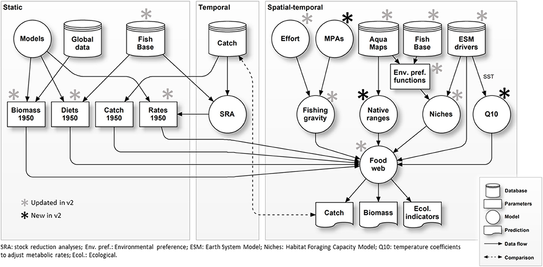
Figure 1. Schematic structure of EcoOcean v2 modeling complex.

An important feature of the food-web model used in EcoOcean was that predator-prey dynamics were based on the “Foraging Arena Theory” (Walters and Juanes, 1993; Ahrens et al., 2012), which added behavior-driven non-linearity to the mass-action terms included in traditional multispecies models. A formal fitting procedure with historical fishing effort and catch data was developed using a customized version of the time-dynamic model Ecosim (Walters et al., 1997) to estimate key vulnerability parameters. This enabled the model to hindcast marine resources and ecosystem services dynamics for the period 1950–2006, projecting the combined impact of environmental parameters and fisheries on global seafood production (Christensen et al., 2015; Lotze et al., 2019) (Supplementary Material A).

Another important feature of EcoOcean v1 was the inclusion of the impact of changes in environmental parameters using the relative habitat capacity of each functional group as a cell-specific attribute through the implementation of the “Habitat Foraging Capacity Model (HFCM)” framework (Christensen et al., 2014) in the spatial-temporal model Ecospace (Walters et al., 1999) through a data exchange engine for Ecospace (Steenbeek et al., 2013). Environmental parameters used to drive cell capacity per functional group were depth, primary production, and sea surface temperature for large pelagic fishes. For depth, information from 1,418 fish and invertebrate species was obtained from FishBase¹ and SeaLifeBase² and was used to define depth distribution based on individual triangular distributions.

The movements of organisms across spatial cells depended on cell suitability and response of organisms to local predation risks and feeding conditions (Walters et al., 1999; Martell et al., 2005; Christensen et al., 2014). When dispersing, species had a higher chance of moving to a neighboring cell if feeding is better, and the risk of depredation lower. To incorporate the active movement of organisms across space, EcoOcean v1 used the dispersal mechanisms established in the spatial-temporal Ecospace model (Walters et al., 1999; Martell et al., 2005). EcoOcean v1 used relative magnitudes of dispersal rates (3, 30, and 300 km/year) representing non-dispersing, demersal, and pelagic groups, respectively, and body-sizes (Martell et al., 2005; Bradbury et al., 2008).

• The fisheries model was based on the existing gravity model implemented in Ecospace, where the effort allocated to each spatial cell is based on the profitability of fishing estimated as the difference between expected income and costs of fishing in each cell (Walters et al., 1999). The cost of fishing was assumed proportional to the distance (km) from the nearest coast. Expected income was estimated using prices per functional groups from a global price database available based on average prices in 2000 (Sumaila et al., 2007).

Time series of fishing effort were obtained from a global spatial effort database that covered 1950 to 2006 and provided information by country and fishing gear specific fleets for 1,365 fleets (Anticamara et al., 2011; Watson et al., 2013). The effort was standardized and the 14 gear types included in the global database were used as global fleets in the fisheries model, which were allocated spatially by LME (Christensen et al., 2015). The effort allocation was set based on historical effort and was scaled per LME as a proportion of the total effort across all fished cells within each LME. The effort included an annual increase of 2% related to technological development (Pauly and Palomares, 2010). Finally, global catch estimates available from the Sea Around Us project (www.seaaroundus.org) were used in two ways: (i) to parameterize the landings by fleet in the initial conditions (1950) and (ii) as observed catches to evaluate the historical model runs from 1951 to 2006 (Christensen et al., 2015).

EcoOcean v2: Key Updates to Further Represent the Global Ocean Dynamics

Here we substantially updated the EcoOcean framework (Figure 1), with the principal aim to (i) improve representation of species contributions to ecosystem dynamics, (ii) improve responses of the marine food web to different environmental drivers, such as changes in sea temperature and primary productivity, and (iii) explore the sensitivity of results to alternative configurations of the ecological model and simulations of climate-change and fishing. These developments were facilitated through the modular design of EcoOcean (Figure 1) and its underlying code structure, which allows access to databases, integration with other models (Steenbeek et al., 2016) and geospatial driver data (Steenbeek et al., 2013; Christensen et al., 2014), and provides control to enable or disable the representation of ecological mechanisms throughout the complex. EcoOcean v2 was implemented in. NET and R software and runs spatial-temporally explicit simulations at 1° spatial resolution, from 1950 to 2100 with monthly time steps.

Improved Representation of Species Contributions

The food web at the core of EcoOcean was extended to explicitly consider over 3,400 individual species (v1 included over 1,400 species-specific information) and better represent marine biodiversity and environmental sensitivities. Species-specific information was added to the functional groups of benthic primary producers, jellyfish, corals, soft corals and sponges, dolphins and porpoises, baleen whales, toothed whales, pinnipeds, and seabirds. Overall, the species resolution contributes to the initial parameterization and spatial-temporal dynamics of each functional group with a weighted average of specific traits (such as biomass, consumption and production rates, catches, environmental tolerances, and preferences, etc.). These modifications to EcoOcean v2 did not change the initial parameterization, but the representation of species within functional groups to explicitly capture diversity in species traits and their contributions to functional group spatial-temporal dynamics.

In addition, a new functional group for marine turtles was added with specific information for the seven living species of marine turtles occurring today.

Improved Responses to Environmental Drivers

Native ranges

When developing global analyses, spatial allocation of species purely based on affinity for habitats, depth and environmental drivers will mean that species may end up at locations where they have never been observed. To account for this, EcoOcean v2 limited the spatial distribution of each species groupings at the start of a simulation with the observed historical native ranges (NR) of its species.

The species groups-wide native ranges were constructed as presence/absence maps from the species within a functional group, and their maximum range extents as defined by Kaschner et al. (2016). These groups-wide native ranges were then incorporated as input capacity layers to the HFCM (Christensen et al., 2014) at the beginning of each spatial-temporal simulation, preventing a species group to occur outside its observed range initially. Within these confines, the species groups were distributed according to affinity for habitats, depth, and environmental drivers. At the end of the first-time simulation step, these range restrictions were released, allowing the species groups to distribute freely according to changing environmental and habitat conditions for the remaining of the simulation (Supplementary Figure 1).

Cell-specific responses

EcoOcean uses the HFCM to determine cell habitat foraging capacity, or cell suitability, per functional group (Christensen et al., 2014) (Supplementary Figure 2). In the HFCM, for each species grouping, cell suitability is the product of three foraging capacity terms: (i) input capacity as obtained from external niche models; (ii) optional foraging capacity derived from affinities for specific habitat types and habitat distributions; and (3) optional functional responses to environmental drivers (Supplementary Figure 1). Cell suitability is expressed as a per-group multiplier to the foraging arena size, thus varying the suitability of a cell for foraging, which then impacts growth and consumption of functional groups.

In EcoOcean, cell suitability was derived from the product of preferences for (or tolerances to) depth, environmental factors (such as temperature), and affinity for specific type of habitat where applicable. Environmental factors change with time and space by driving the HFCM with ESM outputs. Using the HFCM and information about environmental envelopes and response functions available, new response functions to most functional groups were added (Supplementary Table 1).

An important modification to EcoOcean v2 was the ability to evaluate species groups functional responses to temperature based on the probability of presence of a group's species per cell (Supplementary Figure 3). This means that the actual response function to temperature of each functional group changed with space and per time step according to the presumed composition of each group in each cell. As functional groups are expressed globally, but the species within vary greatly in distributions due to individual thermal tolerances, EcoOcean v2 combined groups' species compositions, species' environmental preferences, and species' likelihood of presence to evaluate how well a species group may tolerate local conditions in a cell. Lacking continuous range predictions for species, we numerically resolved this as follows: for each species within a species group, for each cell, tolerance to local temperature was determined from AquaMaps responses to temperature (Kaschner et al., 2016). Only species that exhibited some form of tolerance to the local temperature were considered within that cell. Furthermore, species that natively occur within the cell contributed fully to the group-wide temperature response; species outside their native range contribute for 10% to the group-wide temperature response. As we do not have reliable biomass distribution data for species over time and space, species' contributions to the functional response were currently not weighted by biomass. These assumptions still allow functional groups to move to new areas if and when suitable conditions were to develop (Supplementary Figure 3).

Temperature-adjusted metabolic rates

The global mass-balanced parameters that are used to initialize EcoOcean are a necessary global average, parameterized to a global averaged temperature. However, aerobic metabolism rates of species vary from optimal average temperatures, and species' capacity for activity, growth, and reproduction exhibit a measure of adaptation on exposure to long-term temperature deviations from the mean (Rao and Bullock, 1954; Lefevre, 2016). This means that for global ecosystem models with globally distributed functional groups, global averages or unadjusted averages or species' mass-balanced conditions and parameters only realistically apply to narrow temperature bands around the globe; elsewhere, species' capacity for activity, growth, and reproduction fundamentally differs due to marked changes in environmental conditions.

To take this into account, in EcoOcean v2 we explored the viability of a Q₁₀ approach in a global ecosystem model context by spatially varying the initial mass-balance parameters such as consumption and production rates as a function of near-evolutionary scale average global temperatures (Supplementary Material). The Q₁₀ temperature coefficient is a measure of the rate of change of a biological or chemical system as a consequence of increasing the temperature by 10 °C. Selecting one single Q₁₀ value for an entire ecosystem is incorrect as Q₁₀ values are available for a large number of organisms and can vary substantially (Lefevre et al., 2017). As a first experiment, the current version of EcoOcean v2 used two values of Q₁₀ to represent only differences between fish and macro-invertebrates based on literature estimates (White et al., 2005), while the rest of the functional groups were left unaffected.

Historical fishing effort and spatial management

A new version of a global fishing effort dataset (Rousseau et al., 2019) was used to replace previous estimates incorporated into EcoOcean, extended from 1950 to 2015. We updated the effort allocation per LME as a proportion of total global effort and kept the annual effort creep of 2% (Pauly and Palomares, 2010). A dynamic module to explore the effectiveness of spatial-temporal management measures such as MPAs, seasonal closures or a combination of both, was also added (Figure 1).

Sensitivity to Alternative Configurations of the Ecological Model and Simulations of Climate Change and Fishing

In this study, we used EcoOcean v2 as an experimental modeling platform to investigate the impact on ecological trajectories of alternative configurations of the ecological model, in addition to the impact of combinations of drivers (e.g., changes in ESM inputs and RCP scenarios, under non-fishing and fishing configurations).

In this study we present the results of three experiments, conducted through 13 simulations (Table 1):

TABLE 1

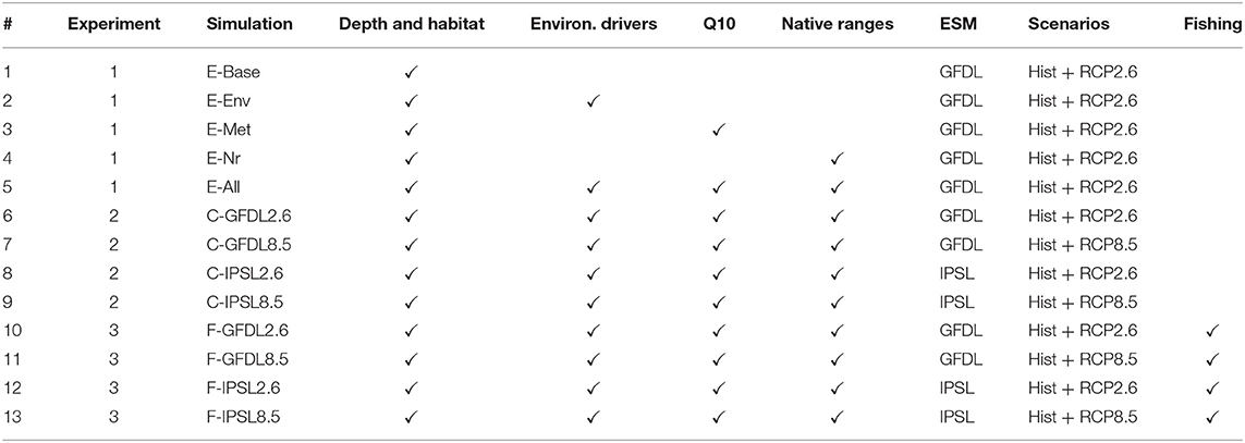
Table 1. EcoOcean experiments and simulations used to test the relative influence of alternative configurations of the ecological model (experiment 1, simulations 1–5), ESM and RCP scenarios (experiment 2, simulations 6–9), and the additional impact of fishing (experiment 3, simulations 10–13) on projected results.

Experiment 1—ecological configurations

We tested the impact of using alternative configurations of the ecological model (or a combination of them) on spatial and temporal trajectories of ecological dynamics. We tested five different main configurations (Table 1): (i) food-web dynamics, habitat affinities and depth preferences as drivers of species distributions, (ii) adding to (i) cell-specific environmental responses to sea surface temperature, (iii) adding to (i) with the Q₁₀ implementation to adjust the temperature-specific metabolic rates, (iv) adding to (i) native ranges constrains to initial conditions, and (v) combining all ecological mechanisms. All these simulations were run from 1950 to 2100 using the same moderate environmental scenario (GFDL ESM2M—Historical/RCP2.6 from CMIP5) (Supplementary Figure 4), considering changes in sea surface temperature and in three primary producers groups (large phytoplankton, small phytoplankton and diazotrophs) driven using the same protocol as in Tittensor et al. (2018). Fishing was disabled.

Experiment 2—climate impacts

We tested how contrasting climate-change scenarios would impact the ecological trajectories of EcoOcean (Table 1) using both GFDL ESM2M—Historical/RCP2.6 and Historical/RCP8.5 and IPSL CMA5-LR—Historical/RCP2.6 and Historical/RCP8.5, both from CMIP5. All these simulations were run from 1950 to 2100 using changes in sea surface temperature and in two or three primary producer groups (large phytoplankton, small phytoplankton, and diazotrophs; this last group was not available for IPSL) (Supplementary Figures 4, 5). Climate change impacts were included through spatial-temporal variability in primary production using the same protocol as in Tittensor et al. (2018), through cell suitability per functional group and through temperature-adjusted metabolic rates as described in previous sections. In this experiment, fishing was disabled.

Experiment 3—fishing impacts

We tested the combined impact of contrasting climate-change scenarios and fishing. We repeated the climate-change scenarios of experiment 2 but added historical fishing effort that was kept constant per LME after 2005 following EcoOcean v1 (Christensen et al., 2015) (Table 1). All these simulations were run from 1950 to 2100 using changes in sea surface temperature and in three primary producer groups (large phytoplankton, small phytoplankton, and diazotrophs) (Supplementary Figures 4, 5). As in experiment 2, climate change impacts were included through spatial-temporal variability in primary production using the same protocol as in Tittensor et al. (2018), through cell suitability per functional group and through temperature-adjusted metabolic rates as described in previous sections.

Spatial-temporal simulations of EcoOcean v2 under the three experiments were run from 1950 to 2100 using a burn-in (or spin-up) period of 10 years and were analyzed via a series of selected standardized aggregated ecological indicators following previous scientific community efforts to compare marine ecosystem modeling outputs (Tittensor et al., 2018) from 1970 to 2100: Total System Biomass (TSB), Total Biomass of Consumers (TBC), Biomass of commercial species (Bcom), Biomass of consumers >10 cm (B10) and Biomass of consumers >30 cm (B30) (Supplementary Table 1). These indicators were initially expressed as t·km². In addition, the biomasses of functional groups or species groupings (organized in various groups of marine mammals, seabirds, marine turtles, elasmobranchs, pelagic and demersal fish, and invertebrates) were used to identify “winners and losers” under climate-change impact and climate-change and fisheries impacts. Results were compared (i) as integrated time series of the global ocean spatial dynamics and (ii) as time series by FAO sub-oceans, both as relative changes with time from year 1970. We also compared results (iii) as annually averaged maps for 1970–1979 and 2090–2099, from where we calculated relative changes computed as (final value-initial value)/initial value ^*100%. The mean and the coefficient of variation were also calculated for aggregated indicators and specific species groupings spatially. Analyses were performed with R version 3.6.3. We used R to plot all the temporal and spatial data. The “ggplot” package (Wickham et al., 2016) was used to apply a smoothing function to capture the general patterns in the temporal trends of biomass, while also reducing the noise. With this methodology, each series show a 95% confidence interval for the original lowess. The “maptools” (Bivand et al., 2020) and “raster” (Hijmans et al., 2015) packages were used to map the spatial-results.

Results

Experiment 1—Ecological Configurations

Temporal Changes

Under the alternative configurations of the ecological model and the same climate-change scenario and absence of fishing, trajectories of ecological indicators resulted in moderate differences of temporal change (Figure 2 and Supplementary Figure 6). Changes were small (±2%) for TSB and TCB indicators, and larger for B10, B30, and Bcom (ranging from −1.5 to +21%) (Table 2a). Overall, changes under configurations E-Env, E-Met, and E-Nr (Table 1) produced projections with small declines by 2100, while the baseline run (E-Base) and the configuration including all the ecological mechanisms (E-All) produced projections with increases by 2100 (Table 2a).

FIGURE 2

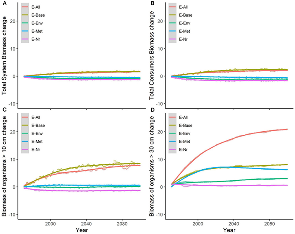
Figure 2. Experiment 1 (Ecological configurations, Table 1)—Relative temporal change of ecological indicators (%) obtained under the different ecological configurations of the model: (A) Total System Biomass, (B) Total Consumer Biomass, (C) Biomass of organisms >10 cm, and (D) Biomass of organisms >30 cm. Supplementary Figure 6 shows results for Biomass of commercial species.

TABLE 2

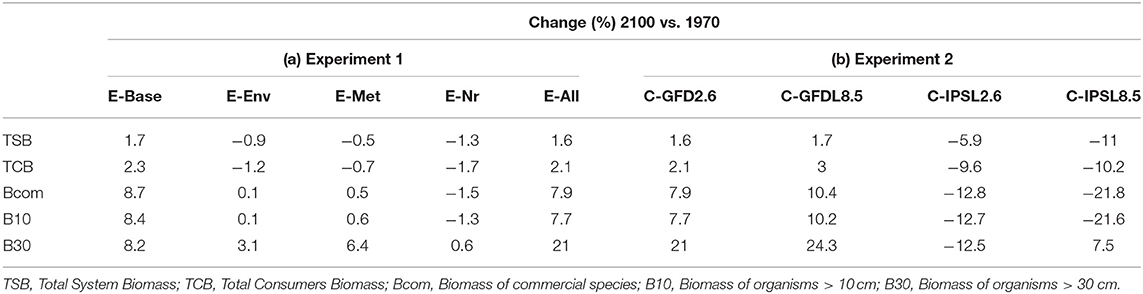
Table 2. (a) Experiment 1 (Ecological configurations, Table 1) and (b) Experiment 2 (Climate impacts, Table 1)—Temporal relative change (%) of ecological indicators between 1970 and 2100 (Figure 2).

Spatial Changes

Our results showed spatial variability of biomass trajectories under the different ecological configurations (Figures 3A,B and Supplementary Figure 7), which was larger in tropical areas (especially in the Indian and Pacific Ocean) and the Poles (Figure 3C). Spatial differences were evident between the different configurations of the model (Supplementary Figure 7), with a concentration of biomass in higher latitude areas under E-Met, and a wider spread of biomass concentrations under E-Env and E-Nr (Table 1). The baseline run (E-Base) presented larger concentrations in specific areas of the Indian and Atlantic Ocean, and the combination of ecological configurations (E-All) showed a gradient of biomass concentration increasing with latitude (Figure 3C). The average change for all five ecological configurations showed negative changes in the tropical areas and positive changes in higher latitude areas (Figure 3D).

FIGURE 3

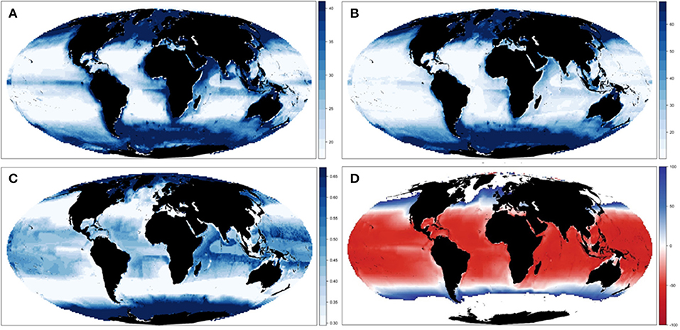
Figure 3. Experiment 1 (Ecological configurations, Table 1)—Spatial changes of Total Consumers Biomass: (A) Mean spatial values across the different ecological configurations and (B) spatial results under configuration E-All in 2001–2005. (C) Coefficient of variation and (D) relative change across the different ecological hypotheses. For visualization purposes, maps (A–C) plot values between the first and third quantile.

Changes by Species Groups

When comparing the outcomes of the alternative configurations of the ecological model, trajectories of biomass by species groups showed larger differences than when examining aggregated ecological indicators. As an example, predicted changes of “Large reef fish” over time showed slight increases under E-Nr and E-All (+5 to +8%) (Table 1), and important declines under the rest of simulations (−35 to −75%) (Figure 4A). Simulations produced also different spatial distributions (Supplementary Figure 8), with larger variability between configurations in coastal areas (Figure 4B). Under E-All, the species tended to increase their biomass in higher latitudes (Figure 4C). The relative change under the five alternative configurations showed overall negative declines in coastal areas with time, with spatial variability depending on the ecological configuration underlying each run (Supplementary Figure 9). While under E-Env and E-Nr the declines were widely distributed, under E-Met they tended to concentrate in high latitude areas. Under E-All, they concentrated in tropical and temperate regions, and increases were projected in northern areas (Figure 4D).

FIGURE 4

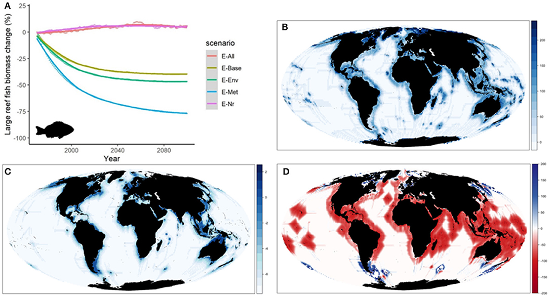
Figure 4. Experiment 1 (Ecological configurations, Table 1)—Changes in “Large reef fish” group: (A) Relative temporal change of biomass (%) obtained under the different ecological configurations of the model from 1970 to 2100, (B) Coefficient of Variation of biomass in 2100 under the different ecological configurations, (C) Biomass (log10) distribution in 2100 under configuration E-All, and (D) Relative change (%) of biomass between 1970 and 2100 under configuration E-All (Fish images source: IAN, 2020).

Summary

Results from the first experiment showed that alternative configurations of the ecological model had moderate effects on aggregated ecological indicators, and larger effects on species projections, even using the same physical and primary producers data (GFDL ESM2M—Historical/RCP2.6) to drive the environmental conditions. Under the simulation that combined the different ecological configurations (E-All) results showed plausible projected patterns in terms of predicted temporal changes and the distribution of biomass of aggregated ecological indicators and of species groupings (Supplementary Figures 7–9).

Experiment 2—Climate Impacts

Temporal Changes

Under the different scenarios of climate-change impacts using the two ESM and RCPs scenarios, without fishing and having all ecological mechanisms enabled, trajectories of ecological indicators resulted in slight to moderate differences of temporal change (Figure 5 and Table 2b). Under GFDL scenarios, relative changes were positive (from +2 to +24%, depending on the indicator). Negative changes were predicted under IPSL scenarios (from −6 to −22%) (with the exception of B30 under RCP8.5). RCP2.6 scenario showed smaller increases under GFDL model and smaller declines under IPSL. Results indicated an amplification of the effect of changes in environmental conditions with larger trophic level organisms (Table 2b), were the moderate negative or positive impacts of aggregated ecological indicators such as TSB or TCB (Figures 5A,B) were larger for Bcom, B10, and B30 (with the exception of B30 under RCP8.5) (Figures 5C,D).

FIGURE 5

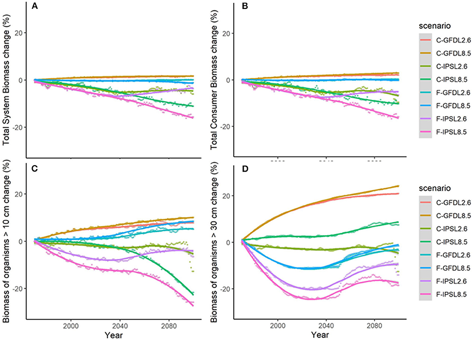
Figure 5. Experiment 2 (Climate impacts) and 3 (Climate impacts and fishing impacts) (Table 1)—Relative temporal change of ecological indicators (%): (A) Total System Biomass, (B) Total Consumer Biomass, (C) Biomass of organisms >10 cm, and (D) Biomass of organisms >30 cm.

Spatial Changes

Results showed noticeable spatial variability of TCB projections under the different climate-change scenarios (Figure 6 and Supplementary Figure 10), which was smaller under GFDL and RCP2.6 scenarios and larger under IPSL and RCP8.5 ones (Supplementary Table 2). The Indian Ocean showed small to moderate declines under all scenarios (from −0.4 to −25%), while the Atlantic regions (including the Mediterranean) and the Central Pacific showed larger declines as we moved from GFDL to IPSL models and from 2.6 to 8.5 RCPs (going from +4 to −34%). On the contrary, the South Pacific and the Antarctic Ocean showed small to moderate increases (from +1 to +30%) (Figure 6 and Supplementary Table 2). TCB showed different areas of negative and positive change depending on the runs, with overall negative changes concentrated in coastal tropical and temperate areas (especially under IPSL model) and positive changes in northern regions and open sea areas (Figure 7), with overall larger declines projected under IPSL (Figures 7C,D). Similar results were recorded for TSB, Bcom, B10, and B30 (Supplementary Table 3).

FIGURE 6

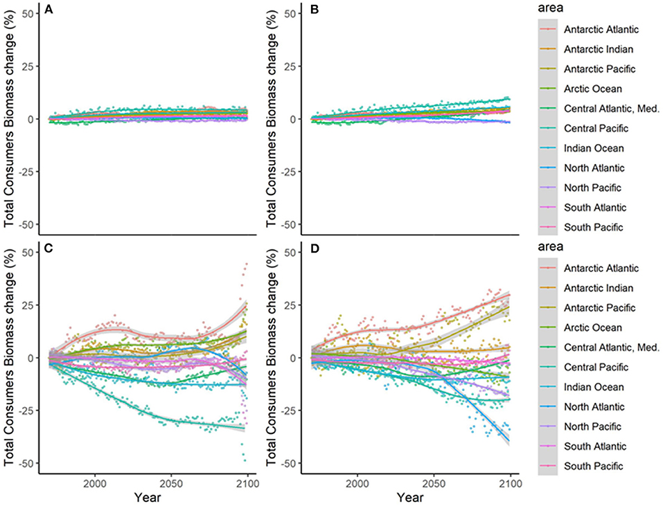
Figure 6. Experiment 2 (Climate impacts, Table 1)—Relative temporal change of Total Consumers Biomass (%) by sub-regional oceans: (A) GFDL RCP2.6; (B) GFDL RCP8.5, (C) IPSL RCP2.6, and (D) IPSL RCP8.5.

FIGURE 7

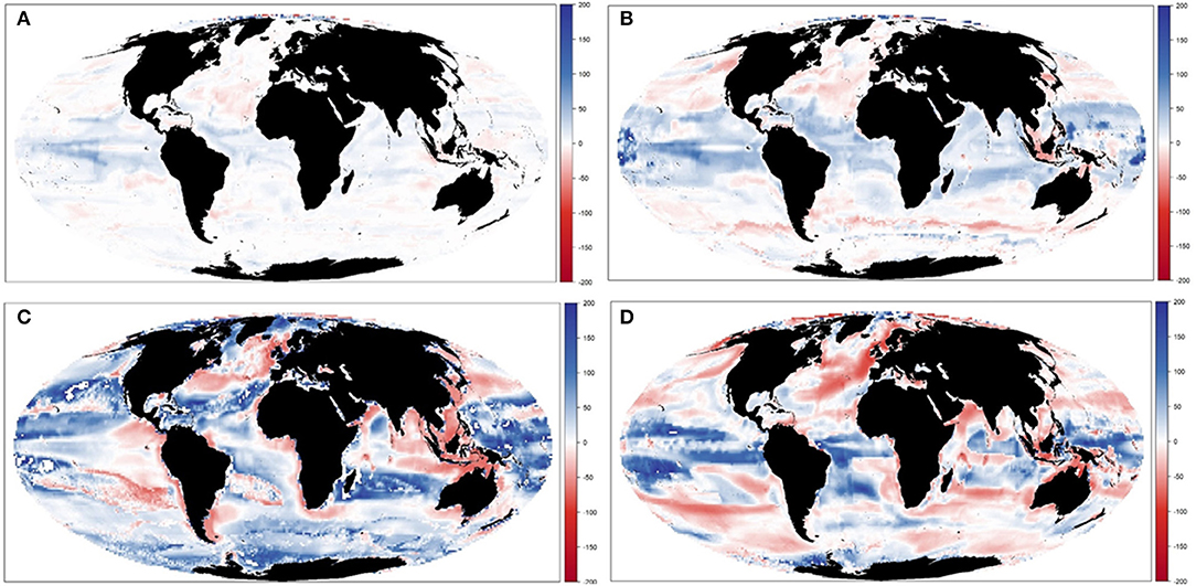
Figure 7. Experiment 2 (Climate impacts, Table 1)—Relative spatial change of Total Consumers Biomass (%) between 1970–1979 and 2090–2099: (A) GFDL RCP2.6; (B) GFDL RCP8.5, (C) IPSL RCP2.6, and (D) IPSL RCP8.5.

Changes by Species Groups

Projections of biomass by species groups resulted in moderate to large temporal differences when comparing the outcomes of the different climate-change scenarios. As an example, trajectories of “Large reef fish” with time (without fishing) showed slight increases under GFDL model and important declines under IPSL one (Figure 8A). Similar patterns were shown for “Small reef fish” (Figure 8B), and “Large sharks” (Figure 8C), while “Small and medium sharks” only showed negative declines under IPSL and RCP8.5 simulation (Figure 8D).

FIGURE 8

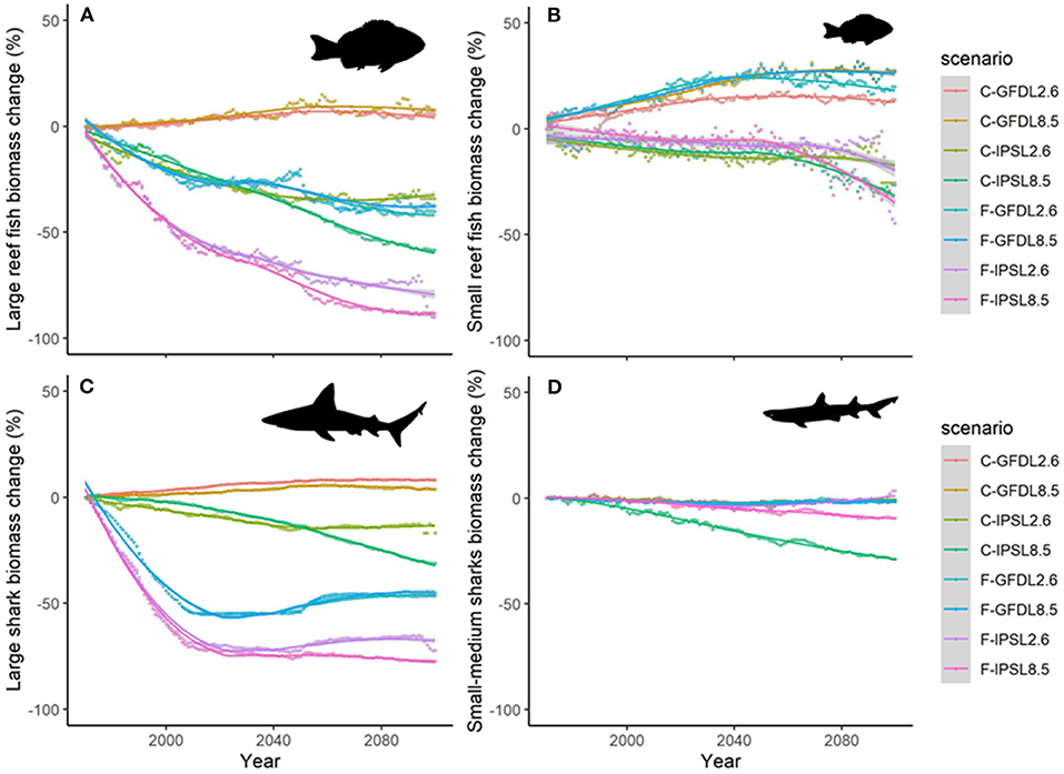
Figure 8. Experiment 2 (Climate impacts) and 3 (Climate impacts and fishing impacts) (Table 1)—Relative temporal biomass change (%) of functional groups: (A) “Large reef fish”, (B) “Small reef fish,” (C) “Large sharks,” and (D) “Small and medium size sharks.” (Fish images source: IAN, 2020).

We observed that IPSL RCP8.5 showed the strongest and most negative effects for species groups (Figure 9 and Supplementary Table 4). Under climate-change impacts, marine mammals, birds, marine turtles, and elasmobranchs showed moderate to large declines in biomass (down to −43%), with the exception of small and medium sharks and rays that showed some biomass increases under GFDL simulations (Figure 9A). Most large pelagic and demersal fish showed large declines as well, especially under IPSL model (with maximum declines for “Large reef fish” of −66%) (Figures 9B,C), with the exception of “Bathydemersal large fish” (which increased from +54 to +100%). On the contrary, medium and small demersal and pelagic fish showed mixed results, with overall increases for “Medium pelagic fishes,” “Bathypelagic medium fishes,” and “Benthopelagic small fish” (Figures 9B,C). These organisms would win under climate-change conditions and no-fishing. Regarding invertebrate groupings, clear declines were projected for “Corals” (to a max. decline of −77%) and “Soft-corals and sponges” (−56%), which decreased strongly in biomass under climate change scenarios. Mixed responses were predicted for molluscs (showing increases of +9% and declines to a max. of −19%), crustaceans and other invertebrates (increases of +60% to declines of −53% depending on the groupings), and an increase of “Other megabenthos species” (with a max of +47% increase) was projected (Figure 9D). Noticeable changes in spatial distributions were also observed for different functional groups, were declines where most profound under IPSL model, and for GFDL RCP8.5 scenario (see example of “Large reef fish” in Supplementary Figures 11, 12).

FIGURE 9

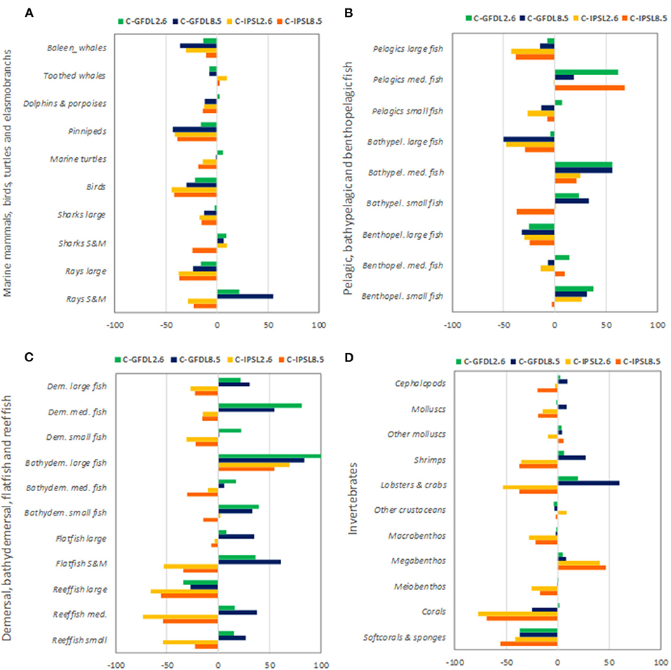
Figure 9. Experiment 2 (Climate impacts, Table 1)—Relative temporal biomass change (%) between 1970 and 2100 by species groupings: (A) Marine mammals, seabirds, marine turtles, and elasmobranchs, (B) Pelagic, bathypelagic, and benthopelagic fish, (C) Demersal, bathydemersal, flatfish, and reef fish, and (D) Invertebrates.

Summary

Results from the second experiment showed that differences in the drivers of climate-change scenarios used under EcoOcean v2 had large impacts on ecological trajectories. The GFDL model produced, overall, less severe negative impacts than IPSL on ecological results. Climate change showed overall negative impacts on larger organisms, and the most pessimistic scenarios of climate impact (RCP8.5) showed the strongest negative effects. These effects were differently distributed in space, with some areas showing clear declines (Indian and Atlantic Oceans) and others showing mostly increases (Antarctic and Arctic Oceans). Climate-change impacts differently affected specific species groupings, with larger organisms showing overall negative trends and smaller organisms showing mixed or positive impacts.

Experiment 3—Climate and Fishing Impacts

Temporal Changes

Under the climate change and fishing impact experiment using the same two ESM and RCPs scenarios and including fishing, trajectories of ecological indicators resulted in smaller positive results under GFDL and larger declines under IPSL (Figure 6, Table 3a, and Supplementary Table 5). The exception was scenario IPSL RCP2.6, which showed the least declines for TSB, TCB, Bcom, and B10 in comparison with the non-fishing configuration.

TABLE 3

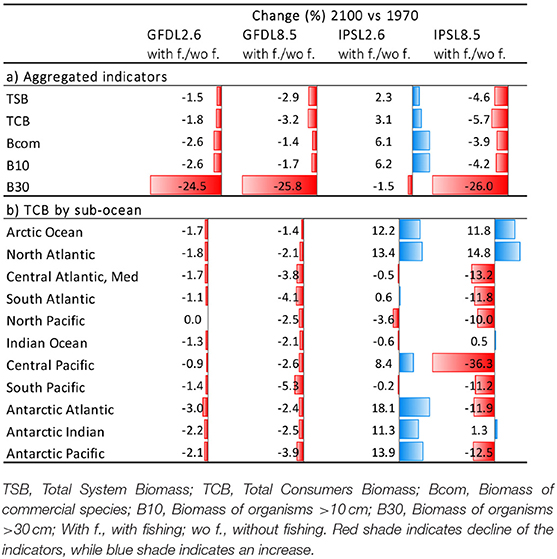
Table 3. Comparison of experiment 2 (Climate impacts) and 3 (Climate and fishing impacts) (Table 1)—(a) Temporal relative change (%) of ecological indicators between 1970 and 2100, and (b) of Total Consumers Biomass (TCB %) under the climate and fishing impact (Figure 10) compared to the climate impact simulations by sub-regional ocean (Figure 6).

Spatial Changes

Results showed large spatial variability of TCB trajectories under the different climate-change and fisheries runs (Figure 10 and Supplementary Figure 13), which was largest under IPSL and RCP8.5 scenarios (Table 3b and Supplementary Table 6). The Central Atlantic region (including the Mediterranean) and the South Pacific showed a decline in indicators under fishing in comparison with the non-fishing configuration in all the simulations (from −0.5 to −13% and from −0.2 to −11%, respectively). This was also the case for most of the sub-regions with some exceptions under IPSL model. For example, the Antarctic regions showed larger increases of TCB under fishing when IPSL RCP2.6 was used, and the Arctic Ocean and North Atlantic when IPSL RCP2.6 and RCP8.5 were used (Table 3b). The average change of TCB showed different areas of negative and positive change depending on the simulation, with larger negative changes concentrated in tropical and temperate areas under IPSL, and positive changes in northern regions and open seas, and overall larger declines predicted under IPSL (Figure 11).

FIGURE 10

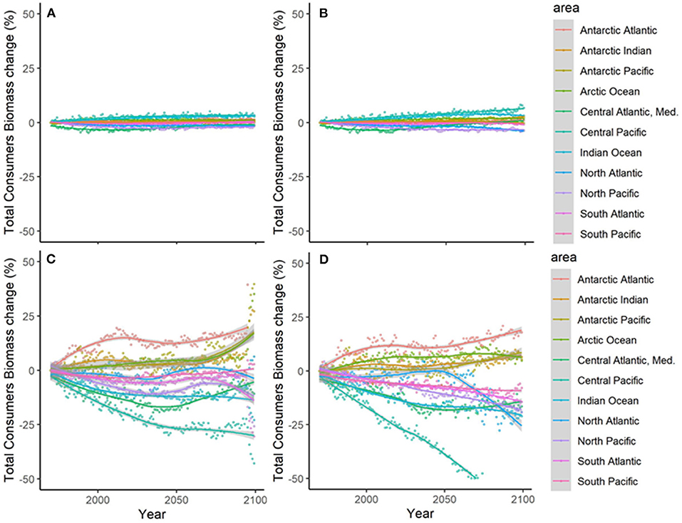
Figure 10. Experiment 3 (Climate impacts and fishing impacts, Table 1)—Relative temporal change of Total Consumers Biomass (%) by sub-regional oceans: (A) GFDL RCP2.6; (B) GFDL RCP8.5, (C) IPSL RCP2.6, and (D) IPSL RCP8.5.

FIGURE 11

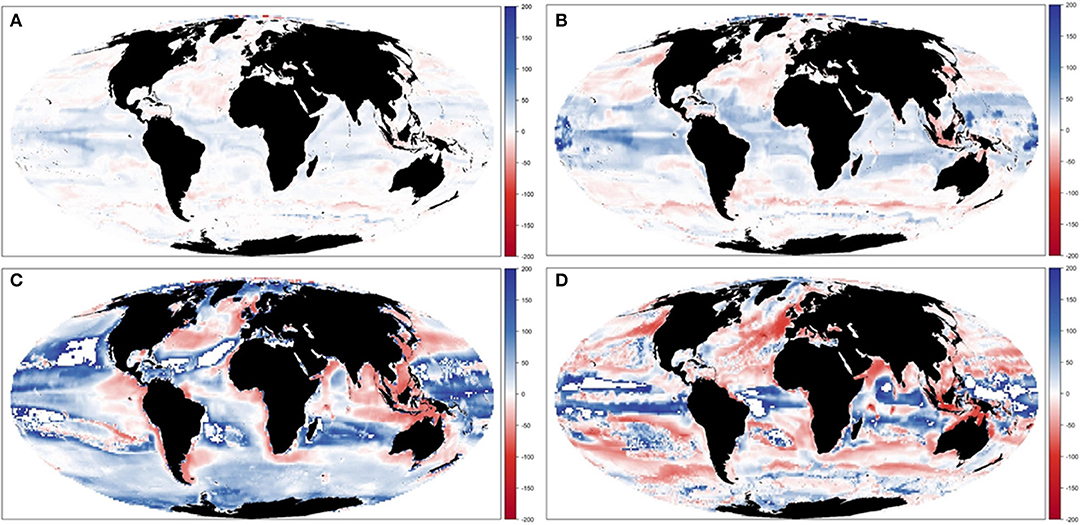
Figure 11. Experiment 3 (Climate impacts and fishing impacts, Table 1)—Relative spatial change of Total Consumers Biomass (%) between 1970–1979 and 2090–2099: (A) GFDL RCP2.6; (B) GFDL RCP8.5, (C) IPSL RCP2.6, and (D) IPSL RCP8.5.

Changes by Species Groups

Trajectories of biomass by species groups resulted in moderate to large temporal differences when comparing the outcomes of the different climate-change scenarios with and without fishing (Table 4 and Supplementary Figure 14). As an example, predicted changes of “Large reef fish” with time showed important declines under fishing in both GFDL and IPSL models (Figure 8A). Similar patterns were shown for “Large sharks” (Figure 8B), while “Small reef fish” and “Small and medium sharks” did not show the same magnitude of declines when fishing was added, and in some cases the trends were reversed (Figures 8C,D).

TABLE 4

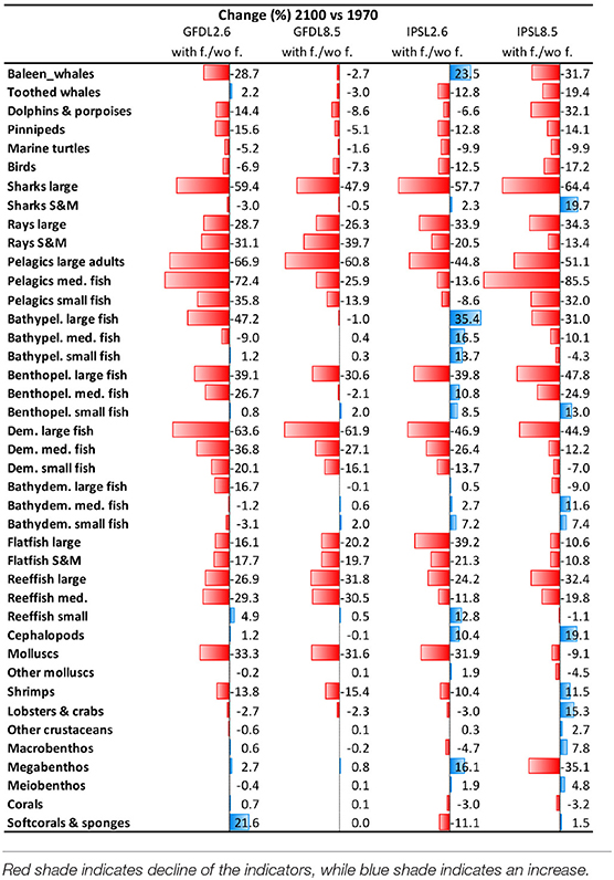
Table 4. Comparison of Experiment 2 (Climate impacts) and 3 (Climate and fishing impacts) (Table 1)—Temporal Change (%) of biomass by functional groups obtained under the climate and fishing impact (Supplementary Figure 14) compared to the climate impact simulations (Figure 9).

We observed that IPSL RCP8.5 scenario showed the strongest and most negative effects for species groups (Table 4, Supplementary Table 7, and Supplementary Figures 14, 15). Under climate change and fisheries impacts, several species that were identified as “losers” under climate-change simulations showed higher declines. This was the case of marine mammals, birds, marine turtles, and elasmobranchs (which declined −80%), with the exception of “Small and medium sharks” under IPSL RCP2.6 (which increased +12%). Declines of biomass from pelagic and demersal fin fish were also stronger under climate change and fishing impact simulations (with declines up to −90% for “Large reef fish” and “Large pelagic fish”). In several cases, smaller species went from increasing under climate-change impacts to decreasing under the cumulative effects of climate change and fishing. This was the case of small and medium pelagic fish groups (from maximums of +7 to minimums of −40%, and max. of +68% to min. of −18%, respectively). Other species groups increased less than under climate-change impacts alone (such as “Bathypelagic medium fish” dropping from +56 to +11%, or “Bathydemersal large fish” dropping from +100 to +45%). There were a few exceptions for organisms that further benefited from fishing: this was the case of “Benthopelagic small fishes” (from −3 to +40%), which showed larger increases under the climate change and fishing simulation (Table 4 and Supplementary Figure 15). Invertebrates showed a variety of mixed responses, with two groups showing clear directions of change: “Molluscs (bivalves)” showed large declines under climate change and fishing (up to −47%), and “Cephalopods” showed further increases (up to +10%) (Supplementary Figure 14d and Supplementary Table 7).

Summary

Results from the third experiment highlighted that combining climate-change and fishing impacts had mostly negative effects on both aggregated ecological indicators and the biomasses of many species groupings, especially for larger-sized species. As in the case of climate-change impact, adding fishing impacts to simulations showed similar results in terms of IPSL RCP8.5, yielding the most pessimistic results. However, some areas showed increases of biomass from a combination of climate change and fishing impacts (Arctic, Antarctic, and North Atlantic) and some smaller-sized organisms showed advantages, such as “Small benthopelagic fish” and “Cephalopods.”

Discussion

We presented a new version of the modeling complex EcoOcean to represent the global marine ecosystem. EcoOcean v2 advances marine ecosystem analyses under multiple and cumulative stressors while explicitly considering species distributions and spatial-temporal food-web dynamics.

We explored the capabilities and sensitivity of the modeling complex through three experiments. We quantified how predicted ecological indicators and species biomasses were influenced by (i) the alternative configurations of specific ecological mechanisms within the ecosystem model, (ii) alternative sets of environmental drivers of climate change accounting for variability in two ESM outputs and RCPs, and (iii) considering human impacts in the form of fishing in addition to climate change.

Our study shows that alternative configurations of the ecological model can have noticeable effects on ecological projections. They were moderate for aggregated ecological indicators such as Total System Biomass (TSB) and Total Consumers Biomass (TCB) and changes in indicators frequently showed similar direction of change. These results stress the importance of model structural uncertainty in EcoOcean v2, as has been previously illustrated for other modeling initiatives (Cheung et al., 2016a; Payne et al., 2016) and when multiple ecosystem models with different setups have been compared (Tittensor et al., 2018; Lotze et al., 2019). The use of aggregated indicators to capture ecological processes at the global level is a practical choice to limit the associated uncertainty of different working hypotheses within complex mechanistic models. These aggregated indicators have been used in recent studies under the Fish-MIP initiative to assess marine animal biomass trajectories under climate change (Tittensor et al., 2018; Lotze et al., 2019).

Effects of structural uncertainty became more evident when looking at indicators that represented larger organisms within the global food web (such as Biomass of organisms larger than 10 or 30 cm, B10 and B30, and Biomass of commercial species, Bcom), or specific species groupings. Our results suggest that informative projections to investigate changes in marine biodiversity must be accompanied by transparent statements about the ecological mechanisms behind model configurations. Community-based ensemble modeling initiatives such as Fish-MIP (Tittensor et al., 2018; Lotze et al., 2019) are designed to capture and compare structural modeling uncertainty deriving from the structural differences of participating Marine Ecosystem Models (MEMs). We believe that transparency about model configuration and ensemble approaches to scenario testing should become the norm for global ecosystem analyses such as the ones performed under IPCC and IPBES (Brondizio et al., 2019; IPCC, 2019).

For the second and third experiment, we used the “full configuration” of EcoOcean v2 in conjunction with different approaches toward climate and fishing. Enabling all ecological mechanisms allowed the model to consider species' responses to fluctuating environmental conditions in combination with affinity for more stable habitats. It also allowed the modeling complex to initialize species to their observed native ranges, from where they could move freely if nearby conditions were to become more suitable. Our first foray into Q₁₀ dynamics enabled the modeling complex some measure of spatial differentiation for growth and production ratios as a function of a near-evolutionary scale average global temperatures. These combined ecological mechanisms produced results that were closer to what we should expect considering historical observations in the distribution of biomass of aggregated ecological indicators and the ecological knowledge of species groupings, while they were also comparable to projections from other modeling initiatives (Lotze et al., 2019).

Our results showed important changes in marine organism biomass distributions, and in ecosystem structure, under various scenarios of climate change. Trends of our projections were in agreement with the vast scientific literature (e.g., Hollowed et al., 2013; Barange et al., 2014; Gattuso et al., 2015; Lotze et al., 2019). Different ESMs and RCPs scenarios had notable impact on EcoOcean projections: while GFDL ESM-2M Hist&RCP scenarios produced more optimistic results, IPSL CMA5-LR Hist&RCP resulted in more pessimistic ones. Simulations under worst-case RCP8.5 emission pathways had extensive (and mostly negative) impacts on ecological properties of the marine ecosystem, while simulations under the most stringent RCP2.6 emission pathways did not experience such large negative effects. This is due to the differences in predicted trends of climate-change effects by the different ESM and RCPs, such as on temperature and phytoplankton growth, which have unique direct and indirect impacts throughout the marine food web (Lotze et al., 2019), and which are mediated by differential growth and consumption rates (Christensen and Walters, 2004). Overall, the impacts of alternative climate-change effects on ecological trajectories were similar or up to a magnitude higher than structural modeling uncertainty. This illustrates that the effect of ESM outputs is at least as important as internal model uncertainty for MEM outputs (e.g., Lotze et al., 2019).

The projected impacts of climate change were unevenly distributed: while some areas showed clear declines (such as the Indian and Atlantic Oceans), others showed increases (Antarctic Ocean). In agreement with previous data analyses and modeling studies, our results suggest that as climate change intensifies, the coastal areas around the tropics and subtropics may become less suitable for a range of species that will disappear from these areas and may be moving to cooler regions (Sunday et al., 2012; Jones and Cheung, 2015; Poloczanska et al., 2016; Bryndum-Buchholz et al., 2019; Link and Watson, 2019; Reygondeau, 2019).

Larger organisms showed overall negative trends, being identified as the “losers” of climate change. Their declines could be mostly attributed to dwindling prey and reduced environmental suitability (Pinsky et al., 2013; Poloczanska et al., 2016). On the contrary, many smaller organisms showed mixed and at times clearly positive impacts—the climate-change “winners.” Some of these smaller organisms benefited from the declines of larger organisms through a reduction in predation pressure, and from density-dependent processes and competition releases as previously illustrated at regional scales (Coll et al., 2008b; Brown et al., 2010; Fulton, 2011). These outcomes illustrate that assessment of the impacts of climate change on marine biodiversity, even in a hypothetical non-fished ocean, should include species interactions to account for non-linear and often surprising consequences (Brown et al., 2010; Fulton, 2011; Fernandes et al., 2013; Christensen et al., 2015). Our results may provide special relevant insights into climate effects on biomass dynamics of data deficient species groupings such as invertebrates (Poloczanska et al., 2016). These results can be of relevance to adapt management strategies and monitoring under a context of climate change.

Our analysis to evaluate how climate-driven responses differed between a hypothetically non-fished and a fished ocean showed that the effect of fishing was mostly negative on aggregated ecological indicators and on the biomass of many—especially larger—species groupings. Fishing generally worsened the conditions already impacted by climate change, even in the cases where climate change benefitted specific groupings of species. These findings are in line with results from a size-based modeling exercise (Blanchard et al., 2012). GFDL ESM-2M Hist&RCP scenarios consistently produced more optimistic results than IPSL CMA5-LR Hist&RCP ones, and RCP8.5 showed the most extreme and mostly negative impacts on ecological projections. Therefore, our results were in agreement with previous studies that show how fishing did not substantially alter the negative direction of climate change effects when looking at total marine animal biomass (Lotze et al., 2019). In addition, the temporal trends for aggregated indicators showed that the additional effect of fishing on climate was not always purely linear but could be non-linear, amplifying the effects of climate, as shown in regional modeling simulations (Fu et al., 2020).

When we analyzed our results by sub-oceans, a larger diversity of cumulative effects of climate change and fishing was observed. Several areas showed further declines of net animal biomass when fishing under climate-change impacts. Some areas, in contrast, showed lower declines or even (modest) gains in total system biomass. In these areas, such as the North Atlantic, fishing has historically been targeting larger organisms and their reduction could have produced a positive effect on mid and small-sized animals through reductions in predation mortality and resource competition (Mackinson et al., 2009; Planque et al., 2010). Increases in catch potential projected in areas of the North Atlantic Ocean (Barange et al., 2014; Peck and Pinnegar, 2019) coincides with our findings.

Species grouping also showed heterogenic responses to climate change and fishing. In essence, we identified four main population responses: (1) losers under climate change that lost more under climate and fishing (“losers that lost more”), (2) winners under climate change that won less under cumulative impacts of climate and fisheries (“winners that won less”), (3) winners under climate change that became losers under cumulative impacts (“winners that became losers”), and (4) winners under climate change that further benefited from fishing impacts (“winners that kept winning”). The “losers that lost more” were mainly large-sized organisms, which have shown historical declines due to fishing (e.g., Christensen et al., 2003; Myers and Worm, 2003). In addition, several organisms that benefited from the impact of climate effects alone “won less” or “became losers” under cumulative effects of climate and fishing. These results illustrate that global fisheries have a negative effect on marine biodiversity and ecosystems in addition to climate change (e.g., Pauly et al., 2002; Worm et al., 2006; Cury and Miserey, 2008; Christensen and Maclean, 2011; Link and Watson, 2019). This is in part related to the spatial congruence and increasing cumulative impact between multiple stressors (Halpern et al., 2015, 2019).

The groups of “Cephalopods” and “Benthopelagic small fish” species were identified to win in a warmer and exploited ecosystem (“winners that kept winning”). This result is especially relevant for monitoring and adaptive management approaches since these groups could become global indicators of cumulative effects of climate and fishing (they could be our “canaries in the environmentally changing marine coal mine”). Our results are in line with a previous global analyses of long-term trends in cephalopod abundance, which showed that cephalopods have increased consistently across taxa from 1960s to 2010 (Doubleday et al., 2016). Modeling studies at local and regional levels showed that cephalopods play a strong ecosystem role (Eddy et al., 2017). Squids, for example, are able to benefit from a general increase in fishing pressure, mainly due to predation release, and exhibit quick responses to changes triggered by the environment, and as such, are very sensitive to changes in fishing and climate change (Coll et al., 2013). Despite this projection of a global increase, cephalopods encompass a large diversity in species, with contrasting ecological strategies (Coll et al., 2013; de la Chesnais et al., 2019). Therefore, differential responses between species of the cephalopod group are expected at the local and regional level (Fulton, 2011).

Benthopelagic small fish are a highly heterogenic group of fishes that live and feed near the bottom of the ocean as well as in midwaters or near the surface and are mostly unexploited. Under climate and fishing impacts they could benefit from a large plasticity, and are able to use different resources from benthic and zooplanktonic organisms, in addition to benefitting from predation release when larger organisms decline. Hypothetically, these organisms are well-positioned to adapt to large changes in the ocean, as previously projected (Christensen et al., 2015), but still too little is known about them. Another interesting result is that “Bathypelagic small fish,” where small mesopelagic fish are included, showed limited biomass increases under both climate and fishing. However, a slight decline is observed under IPSL CMA5-LR RCP8.5 scenario. These results are relevant in the light of their important biomass and key role in supporting the marine ecosystems (Irigoien et al., 2014) and the current discussion about their potential for exploitation vs. sensitivity to cumulative impacts (Hidalgo and Browman, 2019; Martin et al., 2020).

Overall, our results illustrate a variety of complex responses of the marine ecosystem to significant levels of climate change and fishing impacts, which will differ depending on the area and organisms' size and ecology, and can be amplified higher up in the marine food web intensifying predominantly negative impacts. Therefore, cumulative effects of climate change and fisheries can produce a mosaic of “winners,” “losers” and ecological surprises due to synergies, trade-offs, and differential growth and consumption rates of species within food webs (Christensen, 1996; Fulton, 2011; Travis et al., 2014). Identifying, at the global level, which species may decline or benefit from cumulative effects of fishing and climate impacts is highly relevant for policy, although regional and local studies are needed to assess these dynamics in detail, at scales relevant to local ecological and management objectives (e.g., Fulton, 2011; Travers-Trolet et al., 2014).

Our findings underscore that under a pessimistic scenario of climate change (RCP 8.5) and with the current fishing impact projected to be maintained to the future, the majority of marine organisms will show declining trends. These results confirm the current concern about the overall unsustainable levels of global change impacts on marine ecosystems (Gattuso et al., 2015; Díaz et al., 2020) and the need for measures to ensure viable and productive fishing activities in the ocean (Barange et al., 2018). They illustrate the need to act on the implementation of sustainable management options of natural resources, and the effective mitigation and adaptation actions to balance the use and conservation of the natural capital (Duarte et al., 2020).

Future Work

With regards to the alternative configurations of EcoOcean, future studies should further investigate the effects of alternative or complementary ecological mechanisms to advance our understanding of structural model uncertainty (Planque et al., 2011; Payne et al., 2016). For example, future improvements should consider the use of multiple Q₁₀ multipliers in accordance to an expanding body of work (Lefevre et al., 2017), and could incorporate hypotheses of adaptation through evolutionary processes (O'Connor et al., 2012; Miller et al., 2018) and applications of the concept to planktonic groups (Laufkötter et al., 2015). Future iterations could also consider a refinement of cell-specific responses to environmental change based on new theoretical and data analyses (Bernhardt et al., 2018; Burrows et al., 2019), or EcoOcean could drive the internal niche model with outputs from dedicated and independent niche models (Jones and Cheung, 2015; Cheung et al., 2016a; Kaschner et al., 2016; Coll et al., 2019). Last, we could improve our assumptions about species presence by connecting with modeling techniques dedicated to predicting global species distributions under scenarios of environmental change (e.g., Reygondeau, 2019).

Our assessment of climate-change impacts on the global marine ecosystem could be improved by adding additional biodiversity resolution to species groupings and explicitly consider the ecological roles that habitat forming species such as corals, seagrasses, kelp, and other macro-algae play in marine ecosystems, where they can modify direct and indirect ecological interactions (Lotze et al., 2011; Dambacher et al., 2015). The consequences of winners and losers from an ecosystem functioning point of view should be further investigated to assess if the role of species groupings may shift at the global level, as they have been observed to do at regional scales (Bates et al., 2014). In addition, the three-dimensional nature of the ocean is a key feature of the marine ecosystem (Behrenfeld et al., 2019). Our modeling complex indirectly represents the third dimension of depth by vertically stratifying species groupings, their interactions, and the flows of energy and matter. However, the vertical use of the water column may be altered by climate change and future exploitation (Brito-Morales et al., 2020; Jorda et al., 2020; Martin et al., 2020). As new insights into these still underexplored deep-sea habitats become available, future iterations of our work may have to revisit the representation of processes that take place in the water column.

Future iterations of this modeling exercise should include additional physical changes in the ocean to better represent localized stressors such as change in ice cover at high latitude areas that can profoundly affect both the lowest and highest trophic levels of the food web (Stroeve et al., 2012; Wang and Overland, 2012); changes in hypoxic or oxygen-minimum zones and their expansions, which is especially relevant for the tropics (Schmidtko et al., 2017; Breitburg et al., 2018); and changes in ocean pH that can be of special relevance to areas such as the North Atlantic (Peck and Pinnegar, 2019). We should also consider the additional range of mitigation targets after the release of the Shared Socioeconomic Pathways, SSPs (Rogelj et al., 2018), namely RCP1.9, RCP3.4, and RCP7.0., and new outputs of ESMs under CMIP6 (Eyring et al., 2016). Especially relevant is the evaluation of the more ambitious target of RCP 1.9 as the new pathway that focusses on limiting global warming below 1.5°C, the goal of the Paris Agreement (Cheung et al., 2016b; IPCC, 2018).

Future iterations of EcoOcean v2 should also be subjected to rigorous model skill assessments (Olsen et al., 2016). This is still a general Achilles heel of spatial-temporal MEMs, where compounding factors such as their complex parameterization, long run times, and limited access to distributed computing facilities and observational data mean that full uncertainty assessments are rarely undertaken (Hollowed et al., 2013; Fulton et al., 2019; Heymans et al., 2020).

A strength of EcoOcean is that the fishing component is explicitly modeled through fishing fleet dynamics that include the interactions between bio-economics of fishing and the abundance and accessibility to marine resources (Walters et al., 1999). Future interactions of this study will invest in revisiting and complementing the fisheries model. For example, we will update to new versions of catch and fishing effort datasets (Watson, 2017; Watson and Tidd, 2018), new data on illegal, unreported, and unregulated catches, global demands and impacts of marine aquaculture (Pauly and Zeller, 2016; Davies et al., 2019; FAO, 2020) and projections of seafood demand (e.g., Maury et al., 2017; FishMIP—ISIMIP, 2020). Future studies can include the further characterization of ecosystem overfishing at the global level (Coll et al., 2008a; Link and Watson, 2019) and the exploration of alternative pathways to reduce it and avoid it. Our modeling complex could be further complemented with additional anthropogenic impacts such as habitat loss due to the degradation of the deep sea (Mengerink et al., 2014) and marine pollution and eutrophication (Halpern et al., 2015). Past and current spatial-temporal management tools can be now explicitly incorporated in the simulations at any time due to the new management model (Figure 1).

In addition to enhancing the predictive capabilities of EcoOcean v2, and of MEMs in general, the main degradation patterns highlighted by studies such as ours show that the scientific community needs to move toward deploying MEMs to test future scenarios of management and evaluate plausible ecosystem responses. EcoOcean v2 is ready to be used to test alternative plausible actions toward protection, mitigation and adaptation actions (e.g., Gownaris et al., 2019; Jones et al., 2020), and eventually, inform about combined effects of plausible ocean-based solutions to global change (Gattuso et al., 2018).

Data Availability Statement

All data inputs to EcoOcean v2 are either freely available as online databases or available under request from data providers. Results from the 13 runs of EcoOcean v2 presented in this study are available upon request to the lead author. The source code of EcoOcean is available under request to the lead author within a collaborative framework.

Author Contributions

MC, JS, VC, and CW designed research. MC, JS, MP, and VC performed research and analyzed data. All authors wrote the paper.

Funding

This study received funding from the European Union's Horizon 2020 research and innovation programme under grant agreement No. 817578 (TRIATLAS project). Additional financial support was provided by the German Federal Ministry of Education and Research through the Inter-Sectorial Impact Model Intercomparison Project (ISIMIP, Grant 01LS1201A1). HL further acknowledges funding by the Natural Sciences and Engineering Research Council (NSERC) of Canada (RGPIN-2014-04491). DT acknowledges support from the Jarislowsky Foundation. VC received support from the Natural Sciences and Engineering Research Council of Canada (NSERC), Discovery Grant RGPIN-2019-04901.

Conflict of Interest

JB was employed by Mountainsoft.

The remaining authors declare that the research was conducted in the absence of any commercial or financial relationships that could be construed as a potential conflict of interest.

Acknowledgments

The authors acknowledge the key contribution of the Fisheries and Marine Ecosystem Model Intercomparison Project (Fish-MIP) from the Inter-Sectorial Impact Model Intercomparison Project (ISIMIP). Specifically, they would like to thank L. Bopp, J. Dunne, C. Stock, and T. Roy for providing ESM outputs, and M. Büchner, J. Volkholz, and J. Schewe for technical support. They also thank Mary O'Connor for discussions about scaling due to temperature effects, and Cristina Garilao for assistance with AquaMaps modeling.

Supplementary Material

The Supplementary Material for this article can be found online at: https://www.frontiersin.org/articles/10.3389/fmars.2020.567877/full#supplementary-material

Footnotes

1. ^www.fishbase.org

2. ^www.sealifebase.org

References

Abson, D. J., Fischer, J., Leventon, J., Newig, J., Schomerus, T., Vilsmaier, U., et al. (2017). Leverage points for sustainability transformation. Ambio 46, 30–39. doi: 10.1007/s13280-016-0800-y

PubMed Abstract | CrossRef Full Text | Google Scholar

Ahrens, R. N. M., Walters, C. J., and Christensen, V. (2012). Foraging arena theory. Fish Fisher. 13, 41–59. doi: 10.1111/j.1467-2979.2011.00432.x

CrossRef Full Text | Google Scholar

Alder, J., Guénette, S., Beblow, J., Cheung, W., and Christensen, V. (2007). Ecosystem-based global fishing policy scenarios. Fisher. Centre Res. Rep. 15:93. doi: 10.14288/1.0074764

CrossRef Full Text | Google Scholar

Anticamara, J., Watson, R., A, G., and Pauly, D. (2011). Global fishing effort (1950-2010): trends, gaps, and implications. Fisher. Res. 107, 131–136. doi: 10.1016/j.fishres.2010.10.016

CrossRef Full Text | Google Scholar

Barange, M., Bahri, T., Beveridge, M. C., Cochrane, K. L., Funge-Smith, S., and Poulain, F. (2018). “Impacts of climate change on fisheries and aquaculture. Synthesis of current knowledge, adaptation and mitigation options,” in FAO Fisheries and Aquaculture Technical Paper No. 627. (Rome: FAO), 628.

Google Scholar

Barange, M., Merino, G., Blanchard, J., Scholtens, J., Harle, J., Allison, E., et al. (2014). Impacts of climate change on marine ecosystem production in societies dependent on fisheries. Nat. Clim. Chang. 4, 211–216. doi: 10.1038/nclimate2119

CrossRef Full Text | Google Scholar

Barraclough, T. G. (2015). How do species interactions affect evolutionary dynamics across whole communities? Annu. Rev. Ecol. Evol. Syst. 46, 25–48. doi: 10.1146/annurev-ecolsys-112414-054030

CrossRef Full Text | Google Scholar

Bates, A. E., Barrett, N. S., Stuart-Smith, R. D., Holbrook, N. J., Thompson, P. A., and Edgar, G. J. (2014). Resilience and signatures of tropicalization in protected reef fish communities. Nat. Clim. Chang. 4, 62–67. doi: 10.1038/nclimate2062

CrossRef Full Text | Google Scholar

Beaugrand, G., and Kirby, R. R. (2018). How do pelagic species respond to climate change? Theories and observations. Ann. Rev. Mar. Sci. 10, 169–197. doi: 10.1146/annurev-marine-121916-063304

PubMed Abstract | CrossRef Full Text | Google Scholar

Behrenfeld, M. J., Gaube, P., Della Penna, A., O'Malley, R. T., Burt, W. J., Hu, Y., et al. (2019). Global satellite-observed daily vertical migrations of ocean animals. Nature 576, 257–261. doi: 10.1038/s41586-019-1796-9

PubMed Abstract | CrossRef Full Text | Google Scholar

Bernhardt, J. R., Sunday, J. M., Thompson, P. L., and O'Connor, M. I. (2018). Nonlinear averaging of thermal experience predicts population growth rates in a thermally variable environment. Proc. R Soc. B Biol. Sci. 285:20181076. doi: 10.1101/247908

PubMed Abstract | CrossRef Full Text | Google Scholar

Bivand, R., Lewin-Koh, N., Pebesma, E., Archer, E., Baddeley, A., Bearman, N., et al. (2020). Package ‘maptools’. Available online at: https://cranr-projectorg/web/packages/maptools/maptoolspdf

Google Scholar

Blanchard, J. L., Jennings, S., Holmes, R., Harle, J., Merino, G., Allen, J. I., et al. (2012). Potential consequences of climate change for primary production and fish production in large marine ecosystems. Phil. Trans. R Soc. B Biol. Sci. 367, 2979–2989. doi: 10.1098/rstb.2012.0231

PubMed Abstract | CrossRef Full Text | Google Scholar

Blois, J. L., Zarnetske, P. L., Fitzpatrick, M. C., and Finnegan, S. (2013). Climate change and the past, present, and future of biotic interactions. Science 341, 499–504. doi: 10.1126/science.1237184

PubMed Abstract | CrossRef Full Text | Google Scholar

Bonan, G. B., and Doney, S. C. (2018). Climate, ecosystems, and planetary futures: The challenge to predict life in Earth system models. Science 359:eaam8328. doi: 10.1126/science.aam8328

PubMed Abstract | CrossRef Full Text | Google Scholar

Bopp, L., Resplandy, L., Orr, J. C., Doney, S. C., Dunne, J. P., Gehlen, M., et al. (2013). Multiple stressors of ocean ecosystems in the 21st century: projections with CMIP5 models. Biogeosciences 10, 6225–6245. doi: 10.5194/bg-10-6225-2013

CrossRef Full Text | Google Scholar

Bradbury, I. R., Laurel, B., Snelgrove, P. V. R., Bentzen, P., and Campana, S. E. (2008). Global patterns in marine dispersal estimates: the influence of geography, taxonomic category and life history. Proc. Biol. Sci. 275, 1803–1809. doi: 10.1098/rspb.2008.0216

PubMed Abstract | CrossRef Full Text | Google Scholar

Brander, K. (2015). Improving the reliability of fishery predictions under climate change. Curr. Clim. Change Rep. 1, 40–48. doi: 10.1007/s40641-015-0005-7

CrossRef Full Text | Google Scholar

Breitburg, D. L., Levin, L. A., Oschlies, A., Grégoire, M., Chavez, F. P., Conley, D. G., et al. (2018). Declining oxygen in the global ocean and coastal waters. Science 359:eaam7240. doi: 10.1126/science.aam7240

PubMed Abstract | CrossRef Full Text | Google Scholar

Brito-Morales, I., Schoeman, D. S., Garcia Molinos, J., Burrowns, M. T., Klein, C. J., Arafeh-Dalmau, N., et al. (2020). Climate velocity reveals increasing exposure of deep-ocean biodiversity to future warming. Nat. Clim. Chang. 10, 576–581. doi: 10.1038/s41558-020-0773-5

CrossRef Full Text | Google Scholar

Brondizio, E., Settele, J., Díaz, S., and Ngo, H. (2019). Global Assessment Report on Biodiversity and Ecosystem Services of the Intergovernmental Science-Policy Platform on Biodiversity and Ecosystem Services. Bonn: IPBES Secretariat.

Google Scholar

Brown, C. J., Fulton, E. A., Hobday, A. J., Matear, R. J., Possingham, H. P., Bulman, C., et al. (2010). Effects of climate driven primary production change on marine food webs: implications for fisheries and conservation. Glob. Chang. Biol. 16, 1194–1212. doi: 10.1111/j.1365-2486.2009.02046.x

CrossRef Full Text | Google Scholar

Bryndum-Buchholz, A., Tittensor, D., Blanchard, J., Cheung, W., Coll, M., Galbraith, E. D., et al. (2019). 21st century climate change impacts on marine animal biomass and ecosystem structure across ocean basins. Glob. Chang. Biol. 25, 459–472. doi: 10.1111/gcb.14512

PubMed Abstract | CrossRef Full Text | Google Scholar

Burrows, M. T., Bates, A. E., Costello, M. J., Edwards, M., Edgar, G. J., Fox, C. J., et al. (2019). Ocean community warming responses explained by thermal affinities and temperature gradients. Nat. Clim. Chang. 9, 959–963. doi: 10.1038/s41558-019-0631-5

PubMed Abstract | CrossRef Full Text | Google Scholar

CBD (2013). Convention on Biological Diversity. Available online at: http://www.cbd.int (accessed August 1, 2020).

Google Scholar

Cheung, W. W., Jones, M. C., Reygondeau, G., Stock, C. A., Lam, V. W., and Frölicher, T. L. (2016a). Structural uncertainty in projecting global fisheries catches under climate change. Ecol. Model. 325, 57–66. doi: 10.1016/j.ecolmodel.2015.12.018

CrossRef Full Text | Google Scholar

Cheung, W. W., Reygondeau, G., and Frölicher, T. L. (2016b). Large benefits to marine fisheries of meeting the 1.5 C global warming target. Science 354, 1591–1594. doi: 10.1126/science.aag2331

PubMed Abstract | CrossRef Full Text | Google Scholar

Christensen, V. (1996). Managing fisheries involving predator and prey species. Rev. Fish Biol. Fish 6, 417–442. doi: 10.1007/BF00164324

CrossRef Full Text | Google Scholar

Christensen, V., Coll, M., Buszowski, J., Cheung, W., Frölicher, T., Steenbeek, J., et al. (2015). The global ocean is an ecosystem: Simulating marine life and fisheries. Glob. Ecol. Biogeogr. 24 507–517. doi: 10.1111/geb.12281

CrossRef Full Text | Google Scholar

Christensen, V., Coll, M., Steenbeek, J., Buszowski, J., Chagaris, D., and Walters, C. J. (2014). Representing variable habitat quality in a spatial food web model. Ecosystems 17, 1397–1412. doi: 10.1007/s10021-014-9803-3

CrossRef Full Text | Google Scholar

Christensen, V., Guenette, S., Heymans, J. J., Walters, C., Watson, R., Zeller, D., et al. (2003). Hundred-year decline of North Atlantic predatory fishes. Fish Fisher.4, 1–24. doi: 10.1046/j.1467-2979.2003.00103.x

CrossRef Full Text | Google Scholar

Christensen, V., and Maclean, J. (2011). Ecosystem Approaches to Fisheries: A Global Perspective. Cambridge: Cambridge University Press.

Google Scholar

Christensen, V., and Walters, C. (2004). Ecopath with Ecosim: methods, capabilities and limitations. Ecol. Model. 72, 109–139. doi: 10.1016/j.ecolmodel.2003.09.003

CrossRef Full Text | Google Scholar

Christensen, V., Walters, C. J., Ahrens, R., Alder, J., Buszowski, J., Christensen, L. B., et al. (2009). Database-driven models of the world's large Marine ecosystems. Ecol. Model. 220, 1984–1996. doi: 10.1016/j.ecolmodel.2009.04.041

CrossRef Full Text | Google Scholar

Claudet, J., Bopp, L., Cheung, W. W., Devillers, R., Escobar-Briones, E., Haugan, P., et al. (2020). A roadmap for using the UN decade of ocean science for sustainable development in support of science, policy, and action. One Earth 2, 34–42. doi: 10.1016/j.oneear.2019.10.012

CrossRef Full Text | Google Scholar

Coll, M., Libralato, S., Tudela, S., Palomera, I., and Pranovi, F. (2008a). Ecosystem overfishing in the Ocean. PLoS ONE 3:e3881. doi: 10.1371/journal.pone.0003881

PubMed Abstract | CrossRef Full Text | Google Scholar

Coll, M., Navarro, J., Olson, R., and Christensen, V. (2013). Assessing the trophic position and ecological role of squids in marine ecosystems by means of food-web models. Deep Sea Res. II Top. Stud. Oceanogr. 95, 21–36. doi: 10.1016/j.dsr2.2012.08.020

CrossRef Full Text | Google Scholar

Coll, M., Palomera, I., Tudela, S., and Dowd, M. (2008b). Food-web dynamics in the South Catalan Sea ecosystem (NW Mediterranean) for 1978-2003. Ecol. Model. 217, 95–116. doi: 10.1016/j.ecolmodel.2008.06.013

CrossRef Full Text | Google Scholar

Coll, M., Pennino, M. G., Sole, J., Steenbeek, J., and Bellido, J. M. (2019). Predicting marine species distributions: complementarity of food-web and Bayesian hierarchical modelling approaches. Ecol. Model. 405, 86–101. doi: 10.1016/j.ecolmodel.2019.05.005

CrossRef Full Text | Google Scholar

Coll, M., Steenbeek, J., Sole, J., Palomera, I., and Christensen, V. (2016). Modelling the cumulative spatial-temporal effects of environmental factors and fishing in a NW Mediterranean marine ecosystem. Ecol. Model. 331, 100–114. doi: 10.1016/j.ecolmodel.2016.03.020

CrossRef Full Text | Google Scholar

Colloff, M. J., Lavorel, S., Kerkhoff, L. E., Wyborn, C. A., Fazey, I., Gorddard, R., et al. (2017). Transforming conservation science and practice for a postnormal world. Conserv. Biol. 31, 1008–1017. doi: 10.1111/cobi.12912

PubMed Abstract | CrossRef Full Text | Google Scholar

Cury, P., and Miserey, Y. (2008). Une mer Sans Poissons. Paris: Calmann-Lévy.

Google Scholar

Dambacher, J. M., Rothlisberg, P. C., and Loneragan, N. R. (2015). Qualitative mathematical models to support ecosystem-based management of Australia's Northern prawn fishery. Ecol. Appl. 25, 278–298. doi: 10.1890/13-2030.1

PubMed Abstract | CrossRef Full Text | Google Scholar

Davies, I. P., Carranza, V., Froehlich, H. E., Gentry, R. R., Kareiva, P., and Halpern, B. S. (2019). Governance of marine aquaculture: pitfalls, potential, and pathways forward. Marine Policy 104, 29–36. doi: 10.1016/j.marpol.2019.02.054

CrossRef Full Text | Google Scholar

de la Chesnais, T., Fulton, E. A., Tracey, S. R., and Pecl, G. T. (2019). The ecological role of cephalopods and their representation in ecosystem models. Rev. Fish Biol. Fish. 29, 313–334. doi: 10.1007/s11160-019-09554-2

CrossRef Full Text | Google Scholar

Díaz, S., Settele, J., Brondízio, E., Ngo, H., Guèze, M., Agard, J., et al. (2020). Summary for policymakers of the global assessment report on biodiversity and ecosystem services of the Intergovernmental Science-Policy Platform on Biodiversity and Ecosystem Services. Bonn: IPBES secretariat. doi: 10.5281/zenodo3553579

CrossRef Full Text | Google Scholar

Doubleday, Z. A., Prowse, T. A., Arkhipkin, A., Pierce, G. J., Semmens, J., Steer, M., et al. (2016). Global proliferation of cephalopods. Curr. Biol. 26, R406–R407. doi: 10.1016/j.cub.2016.04.002

PubMed Abstract | CrossRef Full Text | Google Scholar

Drakou, E. G., Pendleton, L., Effron, M., Ingram, J. C., and Teneva, L. (2017). When ecosystems and their services are not co-located: oceans and coasts. ICES J. Marine Sci. 74, 1531–1539. doi: 10.1093/icesjms/fsx026

CrossRef Full Text | Google Scholar

Duarte, C. M., Agusti, S., Barbier, E., Britten, G. L., Castilla, J. C., Gattuso, J.-P., et al. (2020). Rebuilding marine life. Nature 580, 39–51.

PubMed Abstract | Google Scholar

du Pontavice, H., Gascuel, D., Reygondeau, G., Maureaud, A., and Cheung, W. W. L. (2020). Climate change undermines the global functioning of marine food webs. Glob. Change Biol. 26, 1306–1318. doi: 10.1111/gcb.14944

PubMed Abstract | CrossRef Full Text | Google Scholar

Eddy, T. D., Lotze, H. K., Fulton, E., Coll, M., Ainsworth, C. H., Neves de Araújo, J., et al. (2017). Ecosystem effects of invertebrate fisheries. Fish Fish. 18, 40–53. doi: 10.1111/faf.12165

CrossRef Full Text | Google Scholar

Eyring, V., Bony, S., Meehl, G. A., Senior, C. A., Stevens, B., Stouffer, R. J., et al. (2016). Overview of the coupled model intercomparison project phase 6 (CMIP6) experimental design and organization. Geosci. Model Dev. 9, 1937–1958. doi: 10.5194/gmd-9-1937-2016

CrossRef Full Text | Google Scholar

FAO (2019). “Report of the expert meeting on other effective area-based conservation measures in the marine capture fishery sector,” in FAO Fisheries and Aquaculture Report No. 1301 (Rome), 74.

Google Scholar

FAO (2020). The State of World Fisheries and Aquaculture. Rome.

Google Scholar

Fernandes, J. A., Cheung, W. W., Jennings, S., Butenschön, M., Mora, L., Frölicher, T. L., et al. (2013). Modelling the effects of climate change on the distribution and production of marine fishes: accounting for trophic interactions in a dynamic bioclimate envelope model. Glob. Chang. Biol. 19, 2596–2607. doi: 10.1111/gcb.12231

PubMed Abstract | CrossRef Full Text | Google Scholar

Fernandes, J. A., Kay, S., Hossain, M. A., Ahmed, M., Cheung, W. W., Lazar, A. N., et al. (2015). Projecting marine fish production and catch potential in Bangladesh in the 21st century under long-term environmental change and management scenarios. ICES J. Marine Sci. 73, 1357–1369. doi: 10.1093/icesjms/fsv217

CrossRef Full Text | Google Scholar

FishMIP—ISIMIP (2020). Fisheries and Marine Ecosystem Model Intercomparison Project. Available online at: https://www.isimip.org/about/marine-ecosystems-fisheries/ (accessed August 1, 2020).

Google Scholar

Fu, C., Xu, Y., Grüss, A., Bundy, A., Shannon, J. L., Heymans, J. J., et al. (2020). Responses of ecological indicators to fishing pressure under environmental change: exploring nonlinearity and threshold. ICES J Marine Sci. 77, 1516–1531. doi: 10.1093/icesjms/fsz182

CrossRef Full Text | Google Scholar

Fulton, B., Blanchard, J., Melbourne-Thomas, J., Plagányi, E. E., and Tulloch, V. J. D. (2019). Where the ecological gaps remain, a modelers' perspective. Front. Ecol. Evol. 7:424. doi: 10.3389/fevo.2019.00424

CrossRef Full Text | Google Scholar

Fulton, E. (2011). Interesting times: winners, losers, and system shifts under climate change around Australia. ICES J. Marine Sci. 68, 1329–1342. doi: 10.1093/icesjms/fsr032

CrossRef Full Text | Google Scholar

Fulton, E. A. (2010). Approaches to end-to-end ecosystem models. J. Marine Syst. 81, 171–183. doi: 10.1016/j.jmarsys.2009.12.012

CrossRef Full Text | Google Scholar

Fulton, E. A., Boschetti, F., Sporcic, M., Jones, T., Little, L. R., Dambacher, J. M., et al. (2015). A multi-model approach to engaging stakeholder and modellers in complex environmental problems. Environ. Sci. Policy 48, 44–56. doi: 10.1016/j.envsci.2014.12.006

CrossRef Full Text | Google Scholar

Galbraith, E., Carozza, D., and Bianchi, D. (2017). A coupled human-Earth model perspective on long-term trends in the global marine fishery. Nat. Commun. 8:14884. doi: 10.1038/ncomms14884

PubMed Abstract | CrossRef Full Text | Google Scholar

Gattuso, J.-P., Magnan, A., Billé, R., Cheung, W. W., Howes, E. L., Joos, F., et al. (2015). Contrasting futures for ocean and society from different anthropogenic CO₂ emissions scenarios. Science 349:aac4722. doi: 10.1126/science.aac4722

PubMed Abstract | CrossRef Full Text | Google Scholar

Gattuso, J.-P., Magnan, A. K., Bopp, L., Cheung, W. W., Duarte, C. M., Hinkel, J., et al. (2018). Ocean solutions to address climate change and its effects on marine ecosystems. Front. Marine Sci. 5:337. doi: 10.3389/fmars.2018.00337

CrossRef Full Text | Google Scholar

Gownaris, N. J., Santora, C. M., Davis, J. B., and Pikitch, E. (2019). Gaps in protection of important ocean areas: a spatial meta-analysis of ten global mapping initiatives. Front. Marine Sci. 6:650. doi: 10.3389/fmars.2019.00650

CrossRef Full Text | Google Scholar

Halpern, B. S., Frazier, M., Afflerbach, J., Lowndes, J. S., Micheli, F., O'Hara, C., et al. (2019). Recent pace of change in human impact on the world's ocean. Sci. Rep. 9:11609. doi: 10.1038/s41598-019-47201-9

PubMed Abstract | CrossRef Full Text | Google Scholar

Halpern, B. S., Frazier, M., Potapenko, J., Casey, K. S., Koenig, K., Longo, C., et al. (2015). Spatial and temporal changes in cumulative human impacts on the world's ocean. Nat. Commun. 6:7615. doi: 10.1038/ncomms8615

PubMed Abstract | CrossRef Full Text | Google Scholar

Heymans, J. J., Bundy, A., Christensen, V., Coll, M., de Mutsert, K., Fulton, E., et al. (2020). The ocean decade: a true ecosystem modelling challenge. Front. Mar. Sci. 554573. doi: 10.3389/fmars.2020.554573

CrossRef Full Text | Google Scholar

Hidalgo, M., and Browman, H. I. (2019). Developing the knowledge base needed to sustainably manage mesopelagic resources. ICES Journal of Marine Science 7, 609–615. doi: 10.1093/icesjms/fsz067

CrossRef Full Text | Google Scholar

Hijmans, R. J., Van Etten, J., Cheng, J., Mattiuzzi, M., Sumner, M., Greenberg, J. A., et al. (2015). Package ‘raster’. R package 734. Available online at: https://cran.r-project.org/web/packages/raster/raster.pdf

Google Scholar

Hoegh-Guldberg, O., and Bruno, J. F. (2010). The impact of climate change on the world's marine ecosystems. Science 328, 1523–1528. doi: 10.1126/science.1189930

PubMed Abstract | CrossRef Full Text | Google Scholar

Hoegh-Guldberg, O., Northrop, E., and Lubchenco, J. (2019). The ocean is key to achieving climate and societal goals. Science 365, 1372–1374. doi: 10.1126/science.aaz4390

PubMed Abstract | CrossRef Full Text | Google Scholar

Hollowed, A. B., Barange, M., Beamish, R. J., Brander, K., Cochrane, K., Drinkwater, K., et al. (2013). Projected impacts of climate change on marine fish and fisheries. ICES J. Marine Sci. 70, 1023–1037. doi: 10.1093/icesjms/fst081

CrossRef Full Text | Google Scholar

IAN (2020). IAN Symbol Libraries. Available online at: https://IAN.umces.edu/symbols/ (accessed August 1, 2020).

Google Scholar

IPCC (2018). Global Warming of 1.5° C: An IPCCSpecial Report on the Impacts of Global Warming of 1.5°C Above Pre-Industrial Levels and Related Global Greenhouse Gas Emission Pathways, in the Context of Strengthening the Global Response to the Threat of Climate Change, Sustainable Development, and Efforts to Eradicate Poverty. Intergovernmental Panel on Climate Change. Available online at: https://www.ipcc.ch/site/assets/uploads/sites/2/2019/06/SR15_Full_Report_Low_Res.pdf

Google Scholar

IPCC (2019). “IPCC special report on the ocean and cryosphere in a changing climate,” in Working Group II Technical Support Unit Intergovernmental Panel on Climate Change, eds H.- O. Pörtner, D. C. Roberts, V. Masson-Delmotte, P. Zhai, M. Tignor, E. Poloczanska, K. Mintenbeck, M. Nicolai, A. Okem, J. Petzold, B. Rama, and N. Weyer. Available online at: https://www.ipcc.ch/site/assets/uploads/sites/3/2019/12/SROCC_FullReport_FINAL.pdf

PubMed Abstract | Google Scholar

Irigoien, X., Klevjer, T. A., Røstad, A., Martinez, U., Boyra, G., Acuña, J., et al. (2014). Large mesopelagic fishes biomass and trophic efficiency in the open ocean. Nat. Commun. 5:4271. doi: 10.1038/ncomms4271

PubMed Abstract | CrossRef Full Text | Google Scholar

Jennings, S., and Collingridge, K. (2015). Predicting consumer biomass, size-structure, production, catch potential, responses to fishing and associated uncertainties in the world's marine ecosystems. PLoS ONE 10:e0133794. doi: 10.1371/journal.pone.0133794

PubMed Abstract | CrossRef Full Text | Google Scholar

Jones, K. R., Klein, C. J., Grantham, H. S., Possingham, H. P., Halpern, B. S., Burgess, N. D., et al. (2020). Area requirements to safeguard Earth's marine species. One Earth 2, 188–196. doi: 10.1016/j.oneear.2020.01.010

CrossRef Full Text | Google Scholar

Jones, M. C., and Cheung, W. W. (2015). Multi-model ensemble projections of climate change effects on global marine biodiversity. ICES J. Marine Sci. 72, 741–752. doi: 10.1093/icesjms/fsu172

CrossRef Full Text | Google Scholar

Jorda, G., Marbà, N., Bennett, S., Santana-Garcon, J., Agusti, S., and Duarte, C. M. (2020). Ocean warming compresses the three-dimensional habitat of marine life. Nat. Ecol. Evol. 4, 109–114. doi: 10.1038/s41559-019-1058-0

PubMed Abstract | CrossRef Full Text | Google Scholar

Kaschner, K., Kesner-Reyes, K., Garilao, C., Rius-Barile, J., Rees, T., and Froese, R. (2016). AquaMaps: Predicted Range Maps for Aquatic Species. World Wide Web Electronic Publication. Available online at: www.aquamaps.org, (accessed August 1, 2020).

Google Scholar

Koenigstein, S., Mark, F. C., Gößling-Reisemann, S., Reuter, H., and Poertner, H. O. (2016). Modelling climate change impacts on marine fish populations: process-based integration of ocean warming, acidification and other environmental drivers. Fish Fish. 17, 972–1004. doi: 10.1111/faf.12155

CrossRef Full Text | Google Scholar

Kroodsma, D. A., Mayorga, J., Hochberg, T., Miller, N. A., Boerder, K., Ferretti, F., et al. (2018). Tracking the global footprint of fisheries. Science 359, 904–908. doi: 10.1126/science.aao5646

PubMed Abstract | CrossRef Full Text | Google Scholar

Laufkötter, C., Vogt, M., Gruber, N., Aita-Noguchi, M., Aumont, O., Bopp, L., et al. (2015). Drivers and uncertainties of future global marine primary production in marine ecosystem models. Biogeosciences 12, 6955–6984. doi: 10.5194/bg-12-6955-2015

CrossRef Full Text | Google Scholar

Lavergne, S., Mouquet, N., Thuiller, W., and Ronce, O. (2010). Biodiversity and climate change: integrating evolutionary and ecological responses of species and communities. Annu. Rev. Ecol. Evol. Syst. 41, 321–350. doi: 10.1146/annurev-ecolsys-102209-144628

CrossRef Full Text | Google Scholar

Lefevre, S. (2016). Are global warming and ocean acidification conspiring against marine ectotherms? A meta-analysis of the respiratory effects of elevated temperature, high CO2 and their interaction. Conserv. Physiol. 4:ow009. doi: 10.1093/conphys/cow009

PubMed Abstract | CrossRef Full Text | Google Scholar

Lefevre, S., McKenzie, D. J., and Nilsson, G. E. (2017). Models projecting the fate of fish populations under climate change need to be based on valid physiological mechanisms. Glob. Chang. Biol. 23, 3449–3459. doi: 10.1111/gcb.13652

PubMed Abstract | CrossRef Full Text | Google Scholar

Levin, L., and Le Bris, N. (2015). The deep ocean under climate change. Science 350, 766–768. doi: 10.1126/science.aad0126

PubMed Abstract | CrossRef Full Text | Google Scholar

Link, J., and Watson, R. A. (2019). Global ecosystem overfishing: clear delineation within real limits to production. Sci. Adv. 5:eaav0474. doi: 10.1126/sciadv.aav0474

PubMed Abstract | CrossRef Full Text | Google Scholar

Link, J. S., Pranovi, F., Libralato, S., Coll, M., Christensen, V., Solidoro, C., et al. (2015). Emergent properties delineate marine ecosystem perturbation and recovery. Trends Ecol. Evol. 30, 649–661. doi: 10.1016/j.tree.2015.08.011

PubMed Abstract | CrossRef Full Text | Google Scholar

Lotze, H. K., Coll, M., Magera, M. A., Ward-Paige, C., and Airoldi, L. (2011). Recovery of marine animal populations and ecosystems. Trends Ecol. Evol. 26, 595–605. doi: 10.1016/j.tree.2011.07.008

PubMed Abstract | CrossRef Full Text | Google Scholar

Lotze, H. K., Tittensor, D. P., Bryndum-Buchholz, A., Eddy, T. D., Cheung, W. L., Galbraith, E. D., et al. (2019). Global ensemble projections reveal trophic amplification of ocean biomass declines with climate change. Proc. Natl. Acad. Sci. U.S.A. 116, 12907–12912. doi: 10.1073/pnas.1900194116

PubMed Abstract | CrossRef Full Text | Google Scholar

Lubchenco, J., and Grorud-Colvert, K. (2015). Making waves: the science and politics of ocean protection. Science 350, 382–383. doi: 10.1126/science.aad5443

PubMed Abstract | CrossRef Full Text | Google Scholar

Mackinson, S., Daskalov, G., Heymans, J. J., Neira, S., Arancibia, H., Zetina-Rejón, M., et al. (2009). Which forcing factors fit? Using ecosystem models to investigate the relative influence of fishing and changes in primary productivity on the dynamics of marine ecosystems. Ecol. Model. 220, 2972–2987. doi: 10.1016/j.ecolmodel.2008.10.021

CrossRef Full Text | Google Scholar

Martell, S. J., Essington, T. E., Lessard, B., Kitchell, J. F., Walters, C. J., and Boggs, C. H. (2005). Interactions of productivity, predation risk, and fishing effort in the efficacy of marine protected areas for the central Pacific. Can. J. Fish. Aquat. Sci. 62, 1320–1336. doi: 10.1139/f05-114

CrossRef Full Text | Google Scholar

Martin, A., Boyd, P., Buesseler, K., Cetinic, I., Claustre, H., Giering, S., et al. (2020). The oceans' twilight zone must be studied now, before it is too late. Nature 580, 26–28. doi: 10.1038/d41586-020-00915-7

PubMed Abstract | CrossRef Full Text | Google Scholar

Maury, O. (2010). An overview of APECOSM, a spatialized mass balanced “Apex Predators ECOSystem Model” to study physiologically structured tuna population dynamics in their ecosystem. Prog. Oceanogr. 84, 113–117. doi: 10.1016/j.pocean.2009.09.013

CrossRef Full Text | Google Scholar

Maury, O., Camplingc, L., Arrizabalaga, H., Aumont, O., Bopp, L., Merino, G., et al. (2017). From shared socio-economic pathways (SSPs) to oceanic system pathways (OSPs): building policy-relevant scenarios for global oceanic ecosystems and fisheries. Glob. Environ. Change 45, 203–216. doi: 10.1016/j.gloenvcha.2017.06.007

CrossRef Full Text | Google Scholar

McCauley, D. J., Pinsky, M. L., Palumbi, S. R., Estes, J. A., Joyce, F. H., and Warner, R. R. (2015). Marine defaunation: animal loss in the global ocean. Science 347, 247–256. doi: 10.1126/science.1255641

PubMed Abstract | CrossRef Full Text | Google Scholar

Mengerink, K., Van Dover, C., Ardron, J., Baker, M., Escobar-Briones, E., Gjerde, K., et al. (2014). A call for deep-ocean stewardship. Science 344, 696–698. doi: 10.1126/science.1251458

PubMed Abstract | CrossRef Full Text | Google Scholar

Miller, D. D., Ota, Y., Sumaila, U. R., Cisneros-Montemayor, A. M., and Cheung, W. W. (2018). Adaptation strategies to climate change in marine systems. Glob. Chang. Biol. 24, e1–e14. doi: 10.1111/gcb.13829

PubMed Abstract | CrossRef Full Text | Google Scholar

Myers, R. A., and Worm, B. (2003). Rapid worldwide depletion of predatory fish communities. Nature 423, 280–283. doi: 10.1038/nature01610

PubMed Abstract | CrossRef Full Text | Google Scholar

Norberg, J., Urban, M. C., Vellend, M., Klausmeier, C. A., and Loeuille, N. (2012). Eco-evolutionary responses of biodiversity to climate change. Nat. Clim. Chang. 2, 747–751. doi: 10.1038/nclimate1588

CrossRef Full Text | Google Scholar

O'Connor, M. I., Holding, J. M., Kappel, C. V., Duarte, C. M., Brander, K., Brown, C. J., et al. (2015). Strengthening confidence in climate change impact science. Glob. Ecol. Biogeogr. 24, 64–76. doi: 10.1111/geb.12218

CrossRef Full Text | Google Scholar

O'Connor, M. I., Selig, E. R., Pinsky, M. L., and Altermatt, F. (2012). Toward a conceptual synthesis for climate change responses. Glob. Ecol. Biogeogr. 21, 693–703. doi: 10.1111/j.1466-8238.2011.00713.x

CrossRef Full Text | Google Scholar

Olsen, E., Fay, G., Gaichas, S., Gamble, R., Lucey, S., and Link, J. S. (2016). sEcosystem model skill assessment. Yes we can! PLoS ONE 11:e0146467. doi: 10.1371/journal.pone.0146467

PubMed Abstract | CrossRef Full Text | Google Scholar

Parmesan, C. (2006). Ecological and evolutionary responses to recent climate change. Annu. Rev. Ecol. Evol. Syst. 37, 637–669. doi: 10.1146/annurev.ecolsys.37.091305.110100

CrossRef Full Text | Google Scholar

Pauly, D., Christensen, V., Guenette, S., Pitcher, T. J., Sumaila, U. R., Walters, C. J., et al. (2002). Towards sustainability in world fisheries. Nature 418, 689–695. doi: 10.1038/nature01017

PubMed Abstract | CrossRef Full Text | Google Scholar

Pauly, D., and Palomares, M. L. D. (2010). An empirical equation to predict annual increases in fishing efficiency. Fisheries Centre Working Paper Series Book 07 (Vancouver, BC).

Google Scholar

Pauly, D., and Zeller, D. (2016). Catch reconstructions reveal that global marine fisheries catches are higher than reported and declining. Nat. Commun. 7:10244. doi: 10.1038/ncomms10244

PubMed Abstract | CrossRef Full Text | Google Scholar

Payne, M. R., Barange, M., Cheung, W. W., MacKenzie, B. R., Batchelder, H. P., Cormon, X., et al. (2016). Uncertainties in projecting climate-change impacts in marine ecosystems. ICES J. Marine Sci. 73, 1272–1282. doi: 10.1093/icesjms/fsv231

CrossRef Full Text | Google Scholar

Peck, M., and Pinnegar, J. K. (2019). “Chapter 5: Climate change impacts, vulnerabilities and adaptations: North Atlantic and Atlantic Arctic marine fisheries,” in Impacts of Climate Change on Fisheries and Aquaculture, eds M. Barange, T. Bahri, M. Beveridge, K. Cochrane, S. Funge-Smith, and F. Poulain (Rome: FAO).

Google Scholar

Peck, M. A., Arvanitidis, C., Butenschön, M., Canu, D. M., Chatzinikolaou, E., Cucco, A., et al. (2016). Projecting Changes in the Distribution and Productivity of Living Marine Resources: A Critical Review of the Suite of Modelling Approaches Used in the Large European Project Vectors. Estuarine: Coastal and Shelf Science.

Google Scholar

Pecl, G. T., Araújo, M. B., Bell, J. D., Blanchard, J., Bonebrake, T. C., Chen, I.-C., et al. (2017). Biodiversity redistribution under climate change: Impacts on ecosystems and human well-being. Science 355:eaai9214. doi: 10.1126/science.aai9214

PubMed Abstract | CrossRef Full Text | Google Scholar

Perry, A. L., Low, P. J., Ellis, J. R., and Reynolds, J. D. (2005). Climate change and distribution shifts in marine fishes. Science 308, 1912–1915. doi: 10.1126/science.1111322

PubMed Abstract | CrossRef Full Text | Google Scholar

Pinsky, M. L., Worm, B., Fogarty, M. J., Sarmiento, J. L., and Levin, S. A. (2013). Marine taxa track local climate velocities. Science 341, 1239–1242. doi: 10.1126/science.1239352

PubMed Abstract | CrossRef Full Text | Google Scholar

Planque, B., Bellier, E., and Loots, C. (2011). Uncertainties in projecting spatial distributions of marine populations. ICES J. Marine Sci. 68, 1045–1050. doi: 10.1093/icesjms/fsr007

CrossRef Full Text | Google Scholar

Planque, B., Fromentin, J. M., Cury, P., Drinkwater, K. F., Jennings, S., Perry, R. I., et al. (2010). How does fishing alter marine populations and ecosystems sensitivity to climate? J. Marine Syst. 79, 403–417. doi: 10.1016/j.jmarsys.2008.12.018

CrossRef Full Text | Google Scholar

Poloczanska, E. S., Brown, C. J., Sydeman, W. J., Kiessling, W., Schoeman, D. S., Moore, P. J., et al. (2013). Global imprint of climate change on marine life. Nat. Clim. Chang. 3, 919–925. doi: 10.1038/nclimate1958

CrossRef Full Text | Google Scholar

Poloczanska, E. S., Burrows, M. T., Brown, C. J., García Molinos, J., Halpern, B. S., Hoegh-Guldberg, O., et al. (2016). Responses of marine organisms to climate change across oceans. Front. Marine Sci. 3:62. doi: 10.3389/fmars.2016.00062

PubMed Abstract | CrossRef Full Text | Google Scholar

Polovina, J. J. (1984). Model of a coral-reef ecosystem 1. The ecopath model and its application to French Frigate Shoals. Coral Reefs 3, 1–11. doi: 10.1007/BF00306135

CrossRef Full Text | Google Scholar

Rao, K. P., and Bullock, T. H. (1954). Q10 as a function of size and habitat temperature in poikilotherms. Am. Nat. 88, 33–44. doi: 10.1086/281806

CrossRef Full Text | Google Scholar

Reygondeau, G. (2019). “Chapter 9: Current and future biogeography of exploited marine exploited groups under climate change,” in Predicting Future Oceans: Sustainability of Ocean and Human Systems Amidst Global Environmental Change, eds A. Cisneros-Montemayor, W. L. Cheung, and Y. Ota (Cambridge, MA: Elsevier).

Google Scholar

Roberts, C. M., O'Leary, B. C., McCauley, D. J., Cury, P. M., Duarte, C. M., Lubchenco, J., et al. (2017). Marine reserves can mitigate and promote adaptation to climate change. Proc. Natl. Acad. Sci. U.S.A. 114, 6167–6175. doi: 10.1073/pnas.1701262114

PubMed Abstract | CrossRef Full Text | Google Scholar

Rogelj, J., Popp, A., Calvin, K. V., Luderer, G., Emmerling, J., Gernaat, D., et al. (2018). Scenarios towards limiting global mean temperature increase below 1.5 C. Nat. Clim. Chang. 8, 325. doi: 10.1038/s41558-018-0091-3

CrossRef Full Text | Google Scholar

Rousseau, Y., Watson, R. A., Blanchard, J. L., and Fulton, E. A. (2019). Evolution of global marine fishing fleets and the response of fished resources. Proc. Natl. Acad. Sci. U.S.A. 116, 12238–12243. doi: 10.1073/pnas.1820344116

PubMed Abstract | CrossRef Full Text | Google Scholar

Sala, O. E., Chapin, F. S., Armesto, J. J., Berlow, E., Bloomfield, J., Dirzo, R., et al. (2000). Biodiversity - global biodiversity scenarios for the year 2100. Science 287, 1770–1774. doi: 10.1126/science.287.5459.1770

PubMed Abstract | CrossRef Full Text | Google Scholar

Scheffers, B. R., De Meester, L., Bridge, T. C., Hoffmann, A. A., Pandolfi, J. M., Corlett, R. T., et al. (2016). The broad footprint of climate change from genes to biomes to people. Science 354:aaf7671. doi: 10.1126/science.aaf7671

PubMed Abstract | CrossRef Full Text | Google Scholar

Schmidtko, S., Stramma, L., and Visbeck, M. (2017). Decline in global oceanic oxygen content during the past five decades. Nature 542, 335–339. doi: 10.1038/nature21399

PubMed Abstract | CrossRef Full Text | Google Scholar

Steenbeek, J., Buszowski, J., Christensen, V., Akoglu, E., Aydin, K., Ellis, N., et al. (2016). Ecopath with Ecosim as a model-building toolbox: source code capabilities, extensions, and variations. Ecol. Model. 319, 178–189. doi: 10.1016/j.ecolmodel.2015.06.031

CrossRef Full Text | Google Scholar

Steenbeek, J., Coll, M., Gurney, L., Melin, F., Hoepffner, N., Buszowski, J., et al. (2013). Bridging the gap between ecosystem modeling tools and geographic information systems: driving a food web model with external spatial–temporal data. Ecol. Model. 263, 139–151. doi: 10.1016/j.ecolmodel.2013.04.027

CrossRef Full Text | Google Scholar

Stenseth, N. C., Mysterud, A., Ottersen, G., Hurrell, J. W., Chan, K.-S., and Lima, M. (2002). Ecological effects of climate fluctuations. Science 297, 1292–1296. doi: 10.1126/science.1071281

PubMed Abstract | CrossRef Full Text | Google Scholar

Stock, C. A., Dunne, J. P., and John, J. G. (2014). Global-scale carbon and energy flows through the marine planktonic food web: an analysis with a coupled physical–biological model. Prog. Oceanogr 120, 1–28. doi: 10.1016/j.pocean.2013.07.001

CrossRef Full Text | Google Scholar

Stroeve, J. C., Serreze, M. C., Holland, M. M., Kay, J. E., Malanik, J., and Barrett, A. P. (2012). The Arctic's rapidly shrinking sea ice cover: a research synthesis. Clim. Change. 110, 1005–1027. doi: 10.1007/s10584-011-0101-1

CrossRef Full Text | Google Scholar

Sumaila, U. R., Marsden, A. D., Watson, R., and Pauly, D. (2007). A global ex-vessel fish price database: construction and applications. J. Bioecon. 9, 39–51. doi: 10.1007/s10818-007-9015-4

CrossRef Full Text | Google Scholar

Sunday, J. M., Bates, A. E., and Dulvy, N. K. (2012). Thermal tolerance and the global redistribution of animals. Nat. Clim. Chang. 2, 686–690. doi: 10.1038/nclimate1539

CrossRef Full Text | Google Scholar

Tittensor, D. P., Eddy, T. D., Lotze, H. K., Galbraith, E. D., Cheung, W., Barange, M., et al. (2018). A protocol for the intercomparison of marine fishery and ecosystem models: fish-MIP v1.0. Geosci. Model Dev. 11, 1421–1442. doi: 10.5194/gmd-11-1421-2018

CrossRef Full Text | Google Scholar

Toonen, R. J., Wilhelm, T. A., Maxwell, S. M., Wagner, D., Bowen, B. W., Sheppard, C. R., et al. (2013). One size does not fit all: the emerging frontier in large-scale marine conservation. Mar. Pollut. Bull. 77, 7–10. doi: 10.1016/j.marpolbul.2013.10.039

PubMed Abstract | CrossRef Full Text | Google Scholar

Travers, M., Shin, Y.-J., Jennings, S., Machu, E., Huggett, J., Field, J., et al. (2009). Two-way coupling versus one-way forcing of plankton and fish models to predict ecosystem changes in the Benguela. Ecol. Model. 220, 3089–3099. doi: 10.1016/j.ecolmodel.2009.08.016

CrossRef Full Text | Google Scholar

Travers-Trolet, M., Shin, Y.-J., Shannon, L. J., Moloney, C. L., and Field, J. G. (2014). Combined fishing and climate forcing in the southern Benguela upwelling ecosystem: an end-to-end modelling approach reveals dampened effects. PLoS ONE 9:e94286. doi: 10.1371/journal.pone.0094286

PubMed Abstract | CrossRef Full Text | Google Scholar

Travis, J., Coleman, F. C., Auster, P. J., Cury, P. M., Estes, J. A., Orensanz, J., et al. (2014). Integrating the invisible fabric of nature into fisheries management. Proc. Natl. Acad. Sci. U.S.A. 111, 581–584. doi: 10.1073/pnas.1305853111

PubMed Abstract | CrossRef Full Text | Google Scholar

Trisos, C. H., Merow, C., and Pigot, A. L. (2020). The projected timing of abrupt ecological disruption from climate change. Nature 580, 496–501. doi: 10.1038/s41586-020-2189-9

PubMed Abstract | CrossRef Full Text | Google Scholar

UN (2020). The UN Sustainable Developmement Goals. Available online at: http://www.un.org/sustainabledevelopment/sustainable-development-goals/ (accessed August 1, 2020).

Google Scholar

Urban, M., Bocedi, G., Hendry, A., Mihoub, J.-B., Pe'er, G., Singer, A., et al. (2016). Improving the forecast for biodiversity under climate change. Science 353:aad8466. doi: 10.1126/science.aad8466

PubMed Abstract | CrossRef Full Text | Google Scholar

Visbeck, M. (2018). Ocean science research is key for a sustainable future. Nat. Commun. 9:690. doi: 10.1038/s41467-018-03158-3

PubMed Abstract | CrossRef Full Text | Google Scholar

Walters, C., Christensen, V., and Pauly, D. (1997). Structuring dynamic models of exploited ecosystems from trophic mass-balance assessments. Rev. Fish Biol. Fish. 7, 139–172. doi: 10.1023/A:1018479526149

CrossRef Full Text | Google Scholar

Walters, C., Pauly, D., and Christensen, V. (1999). Ecospace: prediction of mesoscale spatial patterns in trophic relationships of exploited ecosystems, with emphasis on the impacts of marine protected areas. Ecosystems 2, 539–554. doi: 10.1007/s100219900101

CrossRef Full Text | Google Scholar

Walters, C. J., and Juanes, F. (1993). Recruitment limitation as a consequence of natural selection for use of restricted feeding habitats and predation risk taking by juvenile fishes. Can. J. Fish. Aquat. Sci. 50, 2058–2070. doi: 10.1139/f93-229

CrossRef Full Text | Google Scholar

Walters, C., Christensen, V., Walters, W., and Rose, K. (2010). Representation of multistanza life histories in Ecospace models for spatial organization of ecosystem trophic interaction patterns. Bull. Mar. Sci. 86, 439–459.

Google Scholar

Wang, M., and Overland, J. E. (2012). A sea ice free summer Arctic within 30 years: an update from CMIP5 models. Geophys. Res. Lett. 39. doi: 10.1029/2012GL052868

CrossRef Full Text | Google Scholar

Watson, R. A. (2017). A database of global marine commercial, small-scale, illegal and unreported fisheries catch 1950–2014. Sci. Data 4:170039. doi: 10.1038/sdata.2017.39

PubMed Abstract | CrossRef Full Text | Google Scholar

Watson, R. A., Cheung, W. W. L., Anticamara, J. A., Sumaila, R. U., Zeller, D., and Pauly, D. (2013). Global marine yield halved as fishing intensity redoubles. Fish Fisher. 14, 493–503. doi: 10.1111/j.1467-2979.2012.00483.x

CrossRef Full Text | Google Scholar

Watson, R. A., and Tidd, A. (2018). Mapping nearly a century and a half of global marine fishing: 1869–2015. Marine Policy 93, 171–177. doi: 10.1016/j.marpol.2018.04.023

CrossRef Full Text | Google Scholar

White, C. R., Phillips, N. F., and Seymour, R. S. (2005). The scaling and temperature dependence of vertebrate metabolism. Biol. Lett. 2, 125–127. doi: 10.1098/rsbl.2005.0378

PubMed Abstract | CrossRef Full Text | Google Scholar

Wickham, H., Chang, W., and Wickham, M. H. (2016). Package ‘ggplot2’. Create Elegant Data Visualisations Using the Grammar of Graphics. Vol 2, 1–189. Available online at: https://cran.r-project.org/web/packages/ggplot2/index.html

Google Scholar

Worm, B., Barbier, E. B., Beaumont, N., Duffy, J. E., Folke, C., Halpern, B. S., et al. (2006). Impacts of biodiversity loss on ocean ecosystem services. Science 314, 787–790. doi: 10.1126/science.1132294

PubMed Abstract | CrossRef Full Text | Google Scholar