 Xu Xu
Xu Xu Carsten Lemmen
 Kai W. Wirtz
- Institute of Coastal Research, Helmholtz-Zentrum Geesthacht Zentrum für Material- und Küstenforschung, Geesthacht, Germany
We here assess long-term trends in marine primary producers in the southern North Sea (SNS) with respect to ongoing regional Earth system changes. We applied a coupled high-resolution (1.5–4.5 km) 3d-physical-biogeochemical regional Earth System model that includes an advanced phytoplankton growth model and benthic biogeochemistry to hindcast ecosystem dynamics in the period 1961–2012. We analyzed the simulation together with in situ observations. Coinciding with the decreasing nutrient level at the beginning of the 1990s, we find a surprising increase in phytoplankton in the German Bight, but not in the more offshore parts of the SNS. We explain these complex patterns by a series of factors which are lacking in many state-of-the-art coupled ecosystem models such as changed light availability and physiological acclimation in phytoplankton. We also show that many coastal time-series stations in the SNS are located in small patches where our model predicts an opposite trend than found for the surrounding waters. Together, these findings call for a reconsideration of current modeling and monitoring schemes.
Introduction
Marine phytoplankton constitute the fundamental basis of the marine food web and biogeochemical cycles. Phytoplankton mediates around half of net primary production (NPP) on Earth (Field et al., 1998; Falkowski and Raven, 2007). Changes in primary production impact higher trophic levels, from zooplankton to fish, marine mammals, and seabirds (Chassot et al., 2010; Capuzzo et al., 2018).
Coasts and shelf seas generally reveal higher NPP due to shallower water depth and high nutrient influx by upwelling or river inflow. The North Sea, a shallow shelf sea to the eastern North Atlantic is one of the most utilized and highly productive sea areas in the world (Ducrotoy et al., 2000; Emeis et al., 2015). The southern North Sea (SNS) features low water depth, strong tidal mixing, diminished ocean influence, and high riverine nutrient inflow. Nutrient loads were elevated from the 1950s to the 1980s due to increased wastewater discharge and use of fertilizers (eutrophication) but declined in the recent decades (Painting et al., 2013; Burson et al., 2016) due to regulations and better wastewater treatment.
Nutrient levels, together with light availability, are primordial factors controlling phytoplankton growth. Phytoplankton in coastal areas such as the SNS are thus directly perturbed by human action, but in addition often seem to track climatic changes (Reid et al., 1998; Taylor et al., 2000; Schlüter et al., 2008). A sustainable management of this sea as requested by a number of national and international directives thus needs to disentangle and to attribute observed changes to natural, proximate, and to direct anthropogenic pressures.
Long-term in situ observations of phytoplankton and nutrient concentration are available for a number of sites (Cadee and Hegeman, 2002; Smaal et al., 2013; Desmit et al., 2019), but prior model studies of long-term biomass dynamics (Daewel and Schrum, 2013; Lynam et al., 2017; Capuzzo et al., 2018) have been validated only against sparse data sets, which lack regional details and long-term variability. Moreover, state-of-the-art coupled biogeochemical models often come with a relatively coarse spatial resolution and rarely resolve strong gradients in phytoplankton community composition and ecophysiology. These models thus face difficulties to represent strong coast-to-shelf variability in phytoplankton (Daewel et al., 2015; Ford et al., 2017). As a consequence, the reliability of hindcasted as well as projected trends in coastal ecosystem states is not clear.
In this study, we employ a novel trait-based phytoplankton model embedded into a high-resolution coastal Earth System set-up to simulate long-term (1961–2012) variations of ecosystem states and primary production in the SNS. The trait-based physiological phytoplankton model has been shown to represent major acclimation patterns over time and within the SNS (Kerimoglu et al., 2017; Wirtz, 2019). It is modularly coupled within a coastal Earth system model context also tested in a number of applications. We aim to further investigate the validity of the set-up using a large amount of in situ data for then unraveling the response of phytoplankton biomass to changes in nutrient levels and climate.
Materials and Methods
Numerical Model System
Biogeochemical (BGC) cycling in the SNS is strongly influenced by riverine and open ocean fluxes and mediated by benthic–pelagic exchange. For the numerical description of the SNS biogeochemistry, we employ an application of the Modular System for Shelves and Coasts (MOSSCO, Lemmen et al., 2018), an Earth System Modeling Framework (ESMF, Theurich et al., 2016) software layer that here interlinks the General Estuarine Turbulence Model (GETM, Burchard and Bolding, 2002) with adjacent compartments as described in more detail below: atmospheric physical and chemical forcing, riverine discharges, and two BGC models in the pelagic and in the benthic domain. The latter are represented within the Framework for Aquatic Biogeochemical Modeling (FABM, Bruggeman and Bolding, 2014). This coupled system of hydrodynamics and benthic and pelagic BGC is the core of several published MOSSCO applications for the SNS that describe spatial–temporal patterns in nutrient concentration (Kerimoglu et al., 2017, 2018; Wirtz, 2019), filter-feeder effects on primary productivity (Lemmen, 2018; Slavik et al., 2019), or benthic sediment and biota interaction (Nasermoaddeli et al., 2018).
Hydrodnamics
The General Estuarine Transport Model (GETM, Burchard and Bolding, 2002) is a structured grid three-dimensional coastal ocean model that has been frequently applied in the North Sea (e.g., Stips et al., 2004; Gräwe et al., 2015). It features vertically adaptive layers (Hofmeister et al., 2010) and vertical density and momentum mixing provided by the General Ocean Turbulence Model (GOTM, Burchard et al., 2006). GETM prognostically calculates local sea surface elevation, tidal dry-falling, currents, temperature, salinity, and transports tracers from other components of the coupled system, i.e., the BGC state variables from the pelagic FABM component.
Pelagic Biogeochemistry
For the representation of pelagic BGC and phytoplankton physiology, the Model for Adaptive Ecosystems in Coastal Seas (MAECS, Wirtz and Kerimoglu, 2016; Kerimoglu et al., 2017) was operated as the single module of a FABM pelagic component in the MOSSCO coupled system. MAECS employs a trait-based approach for the optimal allocation between different intracellular machineries (i.e., photo harvesting, electron chain, high number of nutrient uptake systems; major element flows described by MACES are depicted in Supplementary Figure S1). Simulated changes in physiological characteristic such as light affinity or growth rate only partially reflect changes in phytoplankton community structure. Variations in physiology in a single species can be much greater than differences between species (Wirtz and Kerimoglu, 2016), which makes it difficult to reconstruct underlying changes in community structure as often observed through, e.g., shifting diatom-to-flagellate ratios. MAECS realistically simulates observed photo-acclimation patterns and the co-limitation by, e.g., P and N (Wirtz and Kerimoglu, 2016). It includes viral infection as a relevant post-bloom phytoplankton mortality factor and a dependence of carnivory (zooplankton mortality) on light conditions, shallowness as a requirement for visual predation, and the presence of suspension feeders (Wirtz, 2019). MAECS prognostically calculates the states and variable stoichiometry of phytoplankton chlorophyll, P and N in relation to C, and can reproduce meso-scale patterns in chlorophyll and nutrients at several temporal scales (Kerimoglu et al., 2017; Wirtz, 2019). The model has, amongst others, been applied for scenario analyses of nutrient loading for water quality in the SNS (Kerimoglu et al., 2017, 2018) and for investigating the coastal chlorophyll gradient (Lemmen, 2018; Wirtz, 2019).
Benthic Biogeochemistry
Nitrogen, oxygen and carbon cycling in the sea floor are represented by the one-dimensional Ocean Margin Experiment exchange early Diagenesis model (OMExDia, Soetaert et al., 1996), extended for phosphorous by Hofmeister et al. (2014) and Wirtz (2019). Two-way exchange and conversion between the pelagic MAECS and benthic OMExDia models are mediated by a specialized MOSSCO component for benthic–pelagic exchange (Hofmeister et al., 2014; Lemmen et al., 2018). Particulate carbon is fractionated in labile and semilabile components with different mineralization rate and N:C ratio; dissolved nitrogen is represented by ammonium and nitrate. OMExDia resolves both aerobic as well as anaerobic processes in the pore water. Particulate material is bioperturbed, dissolved species are diffused in the vertical dimension, which is discretized with linearly increasing depth layers.
Setup and Boundary Conditions
Our SNS set-up is delineated by the Dutch and German coastline to the South and East, and it has open boundaries to the West (English Channel) and North (open North Sea). It is spatially represented as a 139 × 98 grid with curvilinear projection, with 1.5 km horizontal resolution in the coastal German Bight and up to 4.5 km resolution at the open ocean boundaries (Supplementary Figure S2). Bottom roughness is constant throughout the domain (10–3 m) as proposed by Gräwe et al. (2015). Average water depth is 20 m, and maximum 50 m, which is resolved by 20 terrain-following model layers. Ten river sources, including the German Bight tributaries Elbe and Weser, provide freshwater, total nitrogen, and total phosphorous. The river nutrient data have been compiled from regional government, research institutions, universities and protection organizations and are in detail described by Eisele and Kerimoglu (2015). Sea surface height, climatological temperature, salinity, and hourly meteorological boundary conditions were obtained from the CoastDat II regional climate hindcast based on the models COSMO-CLM, TRIM-NP and HAMSOM (Geyer, 2014)1. A monthly climatology of depth-dependent open ocean boundary conditions for dissolved inorganic N and P was prescribed. This climatology was obtained from Grosse et al., 2016’s ECOHAM (Ecosystem Hamburg) 2000–2010 simulation, which in turn derives from the POLCOMS-ERSEM (Proudman Oceanographic Laboratory Coastal Ocean Modeling System European Regional Seas Ecosystem Model) common boundary condition used in the North Sea ecosystem model comparison by Lenhart et al., 2010. This physical and BGC setup was validated by Kerimoglu et al. (2017). The sediment was constrained by sea bottom temperature from GETM, constant saturated oxygen and porosity ranging from 0.9 to 0.7 in the 15 layers down to 16 cm depth.
Simulations were performed for 1960 through 2012 and evaluated between 1961 and 2012 (52 years). Physical fields were initialized from CoastDat climatological values; pelagic BGC variables were initialized with constant fields from Wirtz and Kerimoglu (2016), and spun up for 1 year (1960, discarded from the analysis), benthic BGC was initialized with an equilibrium steady state derived from a 30-year spin-up; all data were saved at 36-h interval for further analysis. BGC–hydrodynamics coupling timestep was 30 min, internal integration for hydrodynamics 60 s with 4th order Runge-Kutta scheme, for pelagic BGC 480 s with adaptive Euler refinement and 720 s with 4th order Runge-Kutta integration for OMExDia.
All simulations presented here were produced with MOSSCO v1.0.0 (archived at https://doi.org/10.5281/zenodo.438922). All parameter files for the configuration of the coupled system, GETM, MAECS, and OMExDia are archived at https://doi.org/10.5281/zenodo.3688216).
Data Integration
The Continuous Plankton Recorder (CPR) survey, managed by the Sir Alister Hardy Foundation for Ocean Science in the United Kingdom, using self-contained automatic plankton recorders, collects plankton continuously from a standard depth of ∼7 m (Hays and Warner, 1993) along the towed routes (Richardson et al., 2006). It provides a long-term (∼70 years) plankton abundance at fine taxonomic resolution and a comprehensive proxy of epipelagic biomass, which is represented by CPR’s Phytoplankton Colour Index (PCI), often referred to as greenness, at the regional scale (Richardson et al., 2006; McQuatters-Gollop et al., 2015). The PCI is assigned a numerical value to represent the amount of phytoplankton pigment on the sample silk (Colebrook and Robinson, 1965), and it is also considered as the best estimate of total phytoplankton chlorophyll concentration from CPR data as it strongly agrees with chlorophyll measurements from CPR samples (Hays and Lindley, 1994) and with satellite estimates of chlorophyll (Batten et al., 2003; Raitsos et al., 2005).
In this work, we used CPR observations in the standard area D1 and most data in area D2 (Richardson et al., 2006) from 1961 to 2012 (Figure 1, database includes 15,986 samples, Helaouet, 2020)2. We interpolated the PCI to the nearest model grid and compared the annual average of simulated chlorophyll with the corresponding greenness.
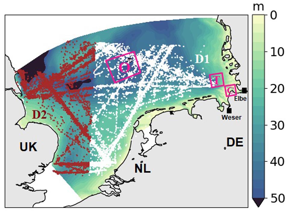
Figure 1. Bathymetry of the model domain, the southern North Sea. Locations of the CPR measurements from the standard CPR area D1 (white dots) and D2 (red dots). Three pink rectangular show the selected analyzed areas, referred to as coast (“C”), transitional (“T”) and offshore (“O”). Black squares indicate the rivers Elbe and Weser.
No CPR data exist for coastal areas shallower than the sampling depth (∼7 m, see Figure 1). To compensate for the spatial blank in CPR data, we applied satellite data in our model–data spatial comparison. The derived chlorophyll of ocean color CCI (Climate Change Initiative) between 1997 and 2012 from the European Space Agency (ESA, available from http://cci.esa.int) were averaged over time to compare with mean simulated Chl. For analyzing the nutrient variations in the transitional area (“T,” section “Variations of Nutrients and Chlorophyll”), regional variations in biomass, and seasonality of nutrients (section “Seasonal Variations of Nutrients and Phytoplankton Biomass”), we used the averages over three typical domains in the SNS that represent the coast–offshore transect from the outer Elbe estuary (denoted “coast” C) to the waters around the island Helgoland (denoted “transitional,” T) in the core of the German Bight to an offshore location in the central SNS (denoted “offshore,” O, Figure 1).
Results
Variations of Nutrients and Chlorophyll
Chlorophyll concentration (Chl) sharply decreases by 70–80% from the coast to the transitional area, both in the simulation and satellite data (Figure 2). The decline is slightly steeper in the simulation, but the relative error between the climatological coastal gradients in observed and simulated Chl distributions rarely exceeds 20%, which for Chl can be regarded as exceptional skill.
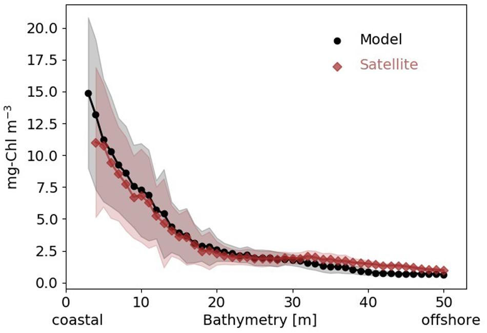
Figure 2. Mean surface Chl concentration (black circles: model simulation, red diamonds: satellite data) 1997–2012 averaged along depth bands from coast to offshore in the SNS. Shading indicates standard deviation within depth band.
The long-term dynamics of simulated Chl tracks the observed dynamics, and the Pearson correlation coefficient between yearly (1961–2012) CPR greenness and model Chl is 0.5 (p < 0.001, n = 15986). The binary segmentation search method reviewed by Truong et al. (2020) indicates a change point in 1986 in both simulated and observed data with higher chlorophyll since 1987 (Figure 3); Mean Chl in the SNS increases from 1.12 mg m–3 (1.07 in greenness) before 1987 to 1.54 mg m–3 (1.82 in greenness) in the recent decades. We therefore partition the data in the two time slices 1961–1986 and 1987–2012 and denote the latter as a high production period.
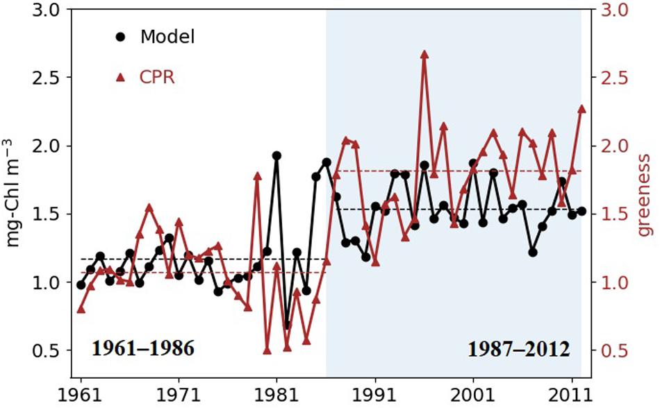
Figure 3. Simulated surface annual mean Chl (black circles) and annual mean CPR greenness (red triangles) in the SNS. Shaded area shows the years after the change point detected by binary segmentation in both simulation and CPR data (1987–2012). Dashed lines are mean values of the two time periods.
Our simulation shows a reduction of mean dissolved inorganic nitrogen (DIN) and dissolved inorganic phosphate (DIP) in the area “T” since the end of 1980s (Figures 4A,B). Interannual variations in simulated DIN and DIP in area “T” track the changes in the observed yearly nutrient load of the rivers Elbe and Weser, which indicate a strong control of nutrient levels by riverine influx. Both DIN and DIP decrease over time, but very differently. Simulated DIN decreases slowly after 1987 and exhibits a ∼7-year oscillation, which may be connected to the NAO pattern in atmospheric precipitation (Visser et al., 1996; Fock, 2003; Radach and Pätsch, 2007). DIP displays a segmented trend with a sharp transition from high values before 1987 to lower ones after 1990. The riverine input strongly decreases (∼50%) from 1987 to 1989, while the negative DIP trend in “T” seems to combine a relatively gentle decrease before 1990 and a sharp drop from 1990 to 1991.
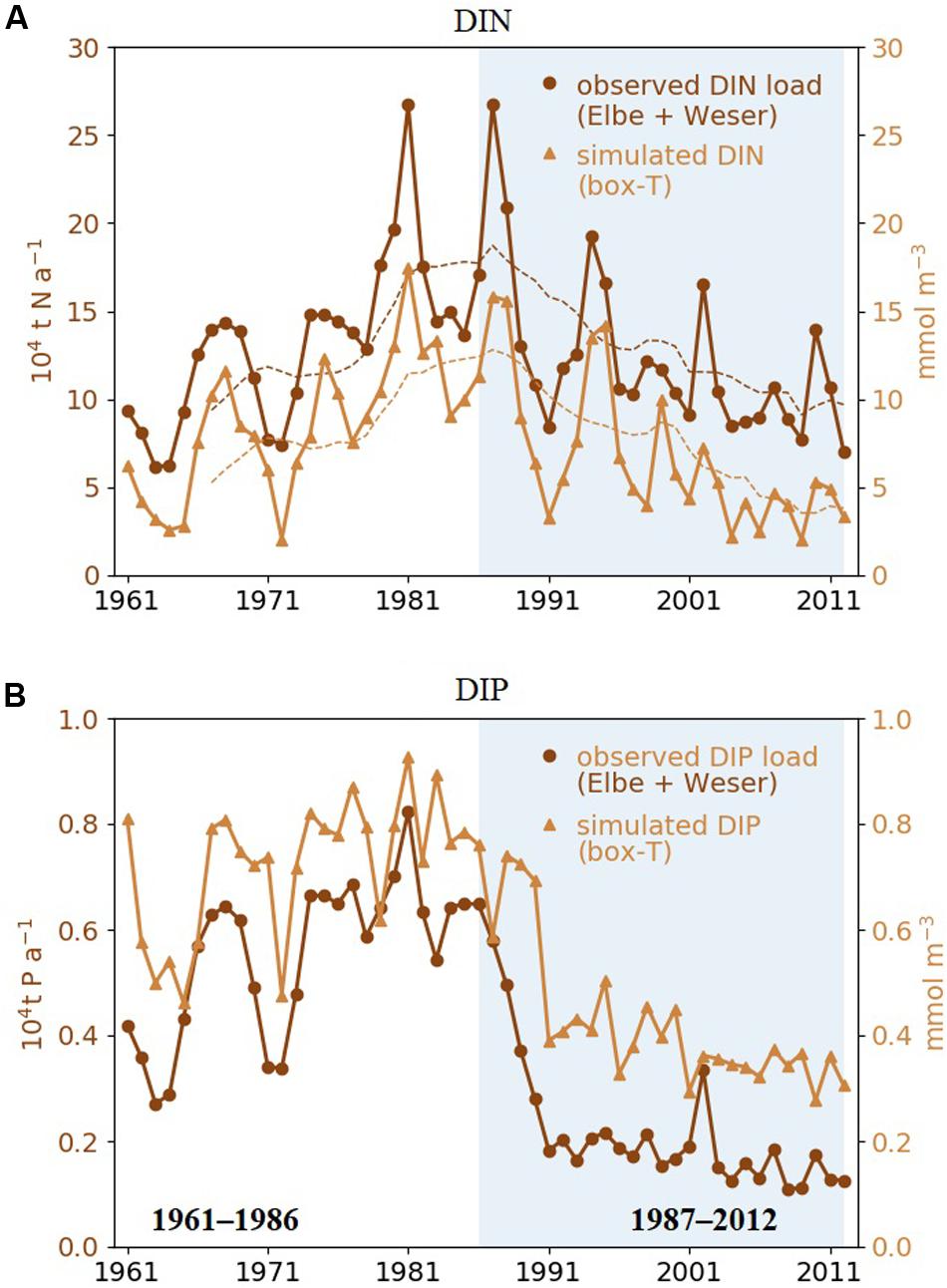
Figure 4. (A) Simulated annual mean DIN concentration averaged over area “T” shown in Figure 1 (yellow triangles) and measured annual total DIN loads of rivers Elbe and Weser (brown circles). Dashed lines are 7-year running means. (B) Same as panel (A), but for DIP. The recent period (1987–2012) are highlighted by shaded areas.
Climatological Changes in Spatial Physical and Biological Distributions
In agreement with the mean cross-sectional distribution for the SNS (Figure 2), Chl along the German, Dutch, and Belgian coasts is much higher (>10 mg m–3) than in most offshore areas (<1 mg m–3, Figure 5A). These high levels of coastal Chl further increase from the 1960–1980s to the 1990–2000s in most southern coastal areas by up to 20% (Figure 5B). In the offshore areas, small decreases in Chl produce high relative changes due to the low concentration there. In most of the western SNS, Chl drops by at most 5%, compared to up to 20% in the eastern SNS.
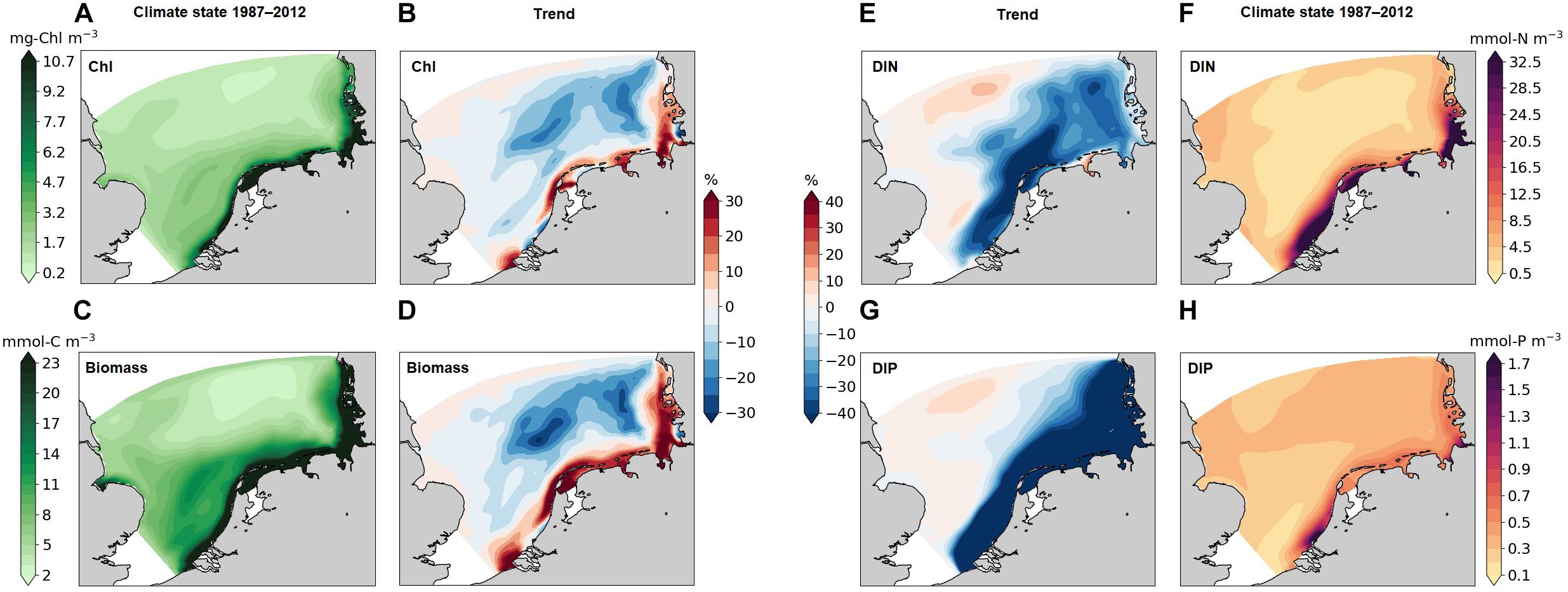
Figure 5. Simulated mean Chl (A), phytoplankton biomass (C), DIN (F), DIP (H) in the time period 1987–2012 averaged over the water column. The trends of Chl (B), phytoplankton biomass (D), DIN (E), DIP (G) denote the difference from the 2nd period (after 1987) to the first one (before 1987).
The phytoplankton biomass distribution (in terms of carbon) exhibits a similar pattern as Chl (Figure 5C). Areas with high biomass (>23 mmol C m–3) are located in a narrow coastal band and overlap with the band of accumulated chlorophyll. The northern water body with low biomass (<5 mmol C m–3) penetrates into the transition zone following the old Elbe river valley. The interdecadal trend of biomass is consistent with the respective chlorophyll trend, but stronger and less confined to the narrow band. There is a strong increase in phytoplankton production in most high biomass areas (more than 30%). A decoupling of the biomass–chlorophyll trend is found in the West-Frisian Wadden Sea, where biomass increases and Chl decreases. At parts of the coast of the southern Netherlands, the northern Elbe estuary, and the Danish coast, chlorophyll decreases much stronger than biomass (Figures 5B,D).
The spatial distributions of dissolved macro-nutrients (DIN and DIP) match the biomass distributions (Figures 5F,H), which decreases from coasts to offshore. Nutrients declined in the recent decades (Figures 5E,G) within the entire southeastern SNS (as exemplified by Figure 4, “T”), in particular, DIP drastically decreases in the whole southern coastal and transitional areas, whereas relative changes in other areas are small. The trends in DIN and DIP are decoupled from phytoplankton biomass in areas “C” and “T” during de-eutrophication. However, for the less productive offshore parts in the eastern SNS, our results display a ∼20% decrease in both biomass and nutrients.
Lateral gradients in annual mean sea surface temperature (SST) in the range from 9 to 11°C are largely determined by the warm tongue of the Atlantic water entering through the English Channel (Figure 6). Winds at 10 m height dominantly come from west (average speed 1.65 m s–1). After 1986, wind speeds increase over the whole model domain (by 0.4 m s–1 on average) while wind direction slightly changes to the north (on average by 4°). In parallel, the Atlantic warm tongue strengthens such that surface waters of the SNS are warmed by around 0.5°C, and the southeastern cold-water body retreats to the shallower areas along the Frisian archipelago and the North Frisian near-shore waters.
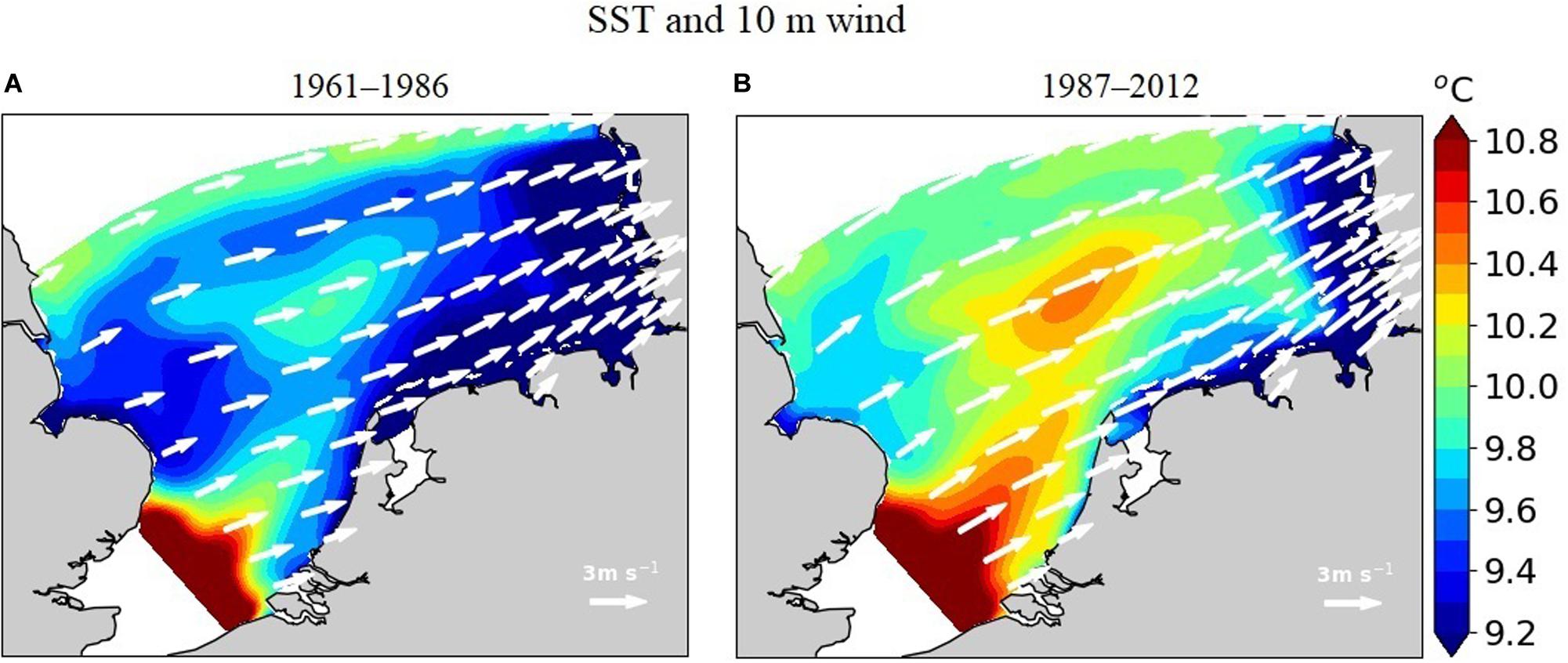
Figure 6. Simulated mean sea surface temperature and 10-m wind speed in (A) 1961–1986 and (B) 1987–2012.
Seasonal Variations of Nutrients and Phytoplankton Biomass
The seasonality in phytoplankton biomass markedly differs between the “C,” “T,” and the “O” areas in both climate states analyzed (Figure 7). In the coast area, simulated phytoplankton growth starts at the end of February, followed by the bloom peak at late March (1961–1986) to late April (1987–2012). From mid-spring to the end of summer, biomass remains high. Bloom timing in transitional waters is similar to the one at the coasts, but biomass drops after the spring bloom and is not sustained throughout the summer. Bloom timing in the offshore domain is delayed by a few days in comparison to the coastal and transitional areas. After a strong post-bloom decline biomass attains even lower values in summer compared to winter concentration due to combined nutrient limitation and zooplankton grazing.
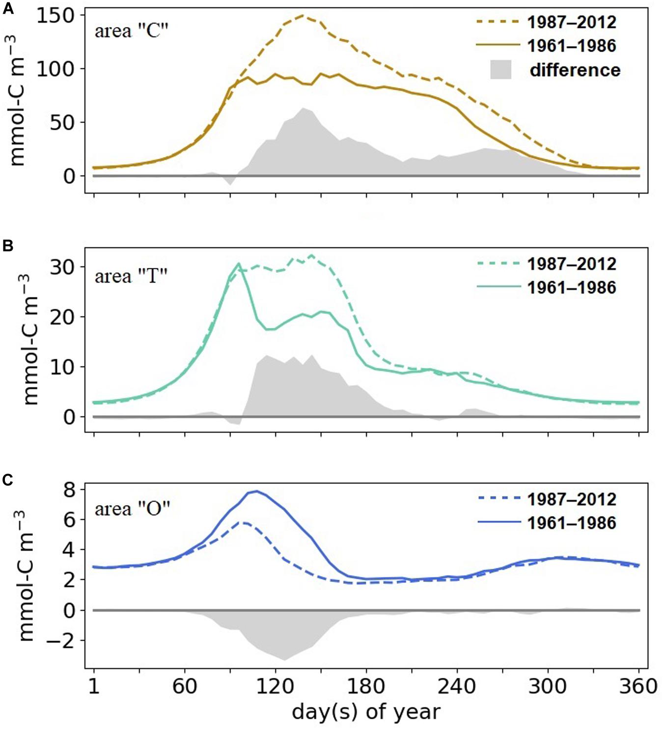
Figure 7. Simulated 6-day mean phytoplankton biomass and changes between 1987–2012 and 1961–1986 (shading) (A) in areas “C,” (B) “T,” (C) and “O.”
Our reconstructed seasonal cycle of phytoplankton reveals long-term changes in terms of both timing and intensity. Despite a very similar timing of the coastal bloom start in 1961–1986 and 1987–2012, the late spring and summer dynamics are different. In the recent decades, the spring peak bloom is much more pronounced (peaking at twice the early period biomass) and has a pronounced maximum in late spring, which slowly declines toward winter. In contrast, the earlier period features a sustained (and lower) maximum biomass until late summer. In the transitional area, the bloom peak is pronounced in 1961–1986 and sustained in the later period, but at the high level of the early period peak. For both the coastal and transitional areas, the spring and summer phytoplankton biomass is much higher in the recent than in the early period. These differences vanish in the offshore area, except for a ∼30% long-term decrease in biomass.
The Chl:C ratio is lower in the period 1987–2012 compared to the earlier period. The decrease reaches up to 25% at the coast in fall, and up to 10% in transitional waters throughout summer and fall (Figure 8A). For DIP, the maximum interdecadal difference occurs in summer, with up to 90% reduction at the coast and 50% reduction in “T” (Figures 8B,C). Similar decreasing trends are found in “C” and “T” DIP concentrations throughout the year in 1987–2012, with greater magnitude in the coastal region, while DIN exhibits richer variability. Coastal DIN concentration does not change between the two analysis periods through the winter and early spring but decreases in summer and fall in the period 1987–2012. The DIN variation in the “T” area reveals a negative long-term trend.
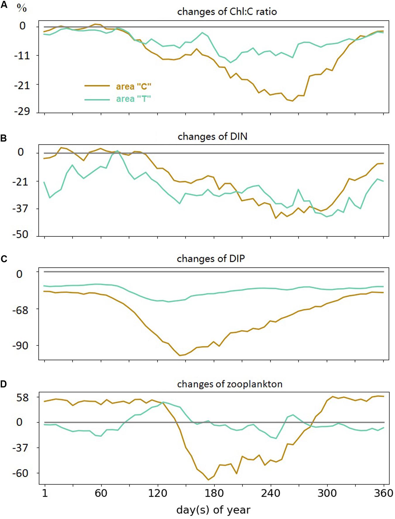
Figure 8. Simulated 6-day variations differences between two periods (1987–2012 – 1961–1982) in panel (A) Chl:C ratio, (B) DIN concentration, (C) DIP concentration, and (D) zooplankton; all in areas “C” and “T” in log-10 scale.
Discussion
The comparison between the satellite-observed Chl, CPR greenness, and the model Chl reconstruction testify the ability of the model system to reproduce spatial, multi-scale patterns and temporal interdecadal dynamics of the SNS very well. The ecosystem model MAECS in particular features a realistic simulation of the coastal Chl gradient, i.e., the increase of Chl from continental shelves toward the coast, which is observed by satellite (Ribalet et al., 2010; Nezlin et al., 2012; Müller et al., 2015), and has already been discussed in terms of phytoplankton growth and mortality factors by Wirtz (2019) for the period 2000–2014. Low light availability in shallow areas is more than compensated by lower grazing losses since zooplankton is in turn subject to high grazing pressure by mussels and juvenile fish. This is confirmed by our analysis: the coastal area displays lower zooplankton abundance after the late 1980s (Figure 8), which in turn can be ascribed to both higher temperature (and thus increased carnivorous losses of herbivores) and lower nutrient concentration propagating to zooplankton production rates.
Historical studies suggest an ecological regime shift in the North Sea in the late 1980s, which involved an increase in phytoplankton biomass (Reid et al., 1998; Beaugrand, 2004; Alheit et al., 2005). In our simulation, we also find a post-1987 biomass increase in the SNS located at coastal to transitional areas. The relative change in costal Chl after the regime shift agrees with the 21% increase according to the long-term chlorophyll data analysis by McQuatters-Gollop et al. (2015). This biological shift coincided with the late 1980s climate regime shift in the extratropical Northern Hemisphere (Lo and Hsu, 2010), which involved the warming in the North Sea (Edwards et al., 2006; van Aken, 2010; Høyer and Karagali, 2016). This climate regime shift is linked to an increase in the NAO index, which is also evidenced by an increased inflow of relatively warm Atlantic water into the SNS (Edwards et al., 2002; Weijerman et al., 2005; Jaagus et al., 2017).
Beside climatic variations, we also simulated de-eutrophication trends in the SNS (van Beusekom et al., 2009; Burson et al., 2016; Meyer et al., 2018). The long-term time series from Helgoland roads station shows that the variabilities and trends of DIN and DIP (Wiltshire et al., 2010) are consistent with those simulated by our model. Kerimoglu et al. (2018) demonstrated the good skill of our model system in simulating recent decade DIN and DIP by comparing to data from Helgoland and four surrounding monitoring stations in the German Bight.
The North Sea ecosystem is commonly considered as resource-controlled (bottom-up, Beaugrand et al., 2009; Olsen et al., 2011). As a consequence, a decline in Chl or primary production in the SNS should be expected due to the reduced riverine loads of nutrients after the late 1980s. This common view is supported by studies that report decreasing Chl at coastal sites (van Beusekom et al., 2009; Desmit et al., 2019). These studies referred to monitoring stations located at Sylt (“L” in Supplementary Figure S3) and very near-shore along the northern (T-10 in Supplementary Figure S3) and southern (NW-02, GR-06 in Supplementary Figure S3) Dutch coast. Our simulation also reveals a local decrease consistent with the observed trends at the locations NW-02 and GR-06, in contrast to the general increase. Simulated offshore decreases are in accordance with both station observations (i.e., NW-70, Supplementary Figure S3) and other model simulations (Daewel and Schrum, 2013; Capuzzo et al., 2018).
The disagreement between the simulation and the station L may be due to the limited model resolution insofar failing to represent physical conditions in the List Tide Basin. The different trends found in station T-10 and in the simulation may indicate the model limitation in resolving differences in BGC processes from the transitional water to offshore as the station is located at the boundary of the two different trends areas. Also, the coarse and parametrized description of turbidity in the model may fail to capture actual spatial–temporal patterns, which act as an important control of near-shore BGC.
The transitional regions are still affected by the input of optically active constituents such as suspended particulate material and colored dissolved organic matter, which strongly limit the light availability for autotrophic growth (Cadee and Hegeman, 2002). In our long-term simulation, the strengthening of westerly winds after 1986 leads to an elevated transport of more clear offshore water into the “T” area, thereby increasing light availability. In the model simulation, this improvement triggers a decreased Chl:C ratio in “T.” Acclimation in Chl:C allows the typically light-limited coastal to transitional phytoplankton to more effectively utilize low nutrient concentration. In addition, the “T” area is located in an intermittently stratified region (van Leeuwen et al., 2015; Capuzzo et al., 2018). The increase in biomass after 1986 occurs mainly in spring, parallel to small changes in stratification intensity. We find a strengthening of stratification (defined as in Lowe et al., 2009) near Helgoland in early spring (Supplementary Figure S4), which is related to increased water column stability and better light availability (Bopp et al., 2001), and thus a higher bloom peak. In summer, however, stratification has been suggested to increase only in the northern North Sea, while decreasing in the SNS (Emeis et al., 2015).
The relative increase in simulated phytoplankton biomass at the coast is higher than in the transitional region. The differential trend reflects differences in winter concentration of DIN, which stays invariant at the coast (“C”) but decreases in the transitional sea (“T”). This reduction in winter DIN in transitional water partially compensates the effect of the improved light environment and weakens primary production.
These regional differences in trends between models, but also between observations at different locations in the SNS underline the relevance of high-resolution spatial monitoring for assessing trends directly and for validating models. We confirm earlier findings on long-term changes in biomass and productivity for the offshore SNS but reveal a more complex picture for near-shore and transitional waters. The latter host the highest productivity in the SNS (Lemmen, 2018; Slavik et al., 2019) so that the opposing trend here cannot be simply neglected.
The reliability of models and set-ups demonstrated for hindcast studies is critical for making future projections (e.g., Wakelin et al., 2015; Holt et al., 2016; Daewel and Schrum, 2017). Our study has identified benchmarks in terms of relevant spatial–temporal BGC patterns such as Chl accumulation in turbid near-coast waters, or the biomass increase in coastal to transitional waters after the onset of de-eutrophication. If these patterns cannot be reproduced, it may be still too early to generate future scenarios.
A high-resolution physical model set-up that extends into very shallow water and is able to represent areas of the coast that are dry during low tide (such as GETM, in our case) is clearly needed for simulating coastal dynamics. In addition, advanced ecosystem models, which differ from classical NPZD-type models may be required to catch essential response mechanisms. For example, we found as key for simulating highly variable coastal–shelf ecosystems the capability to resolve acclimation in phytoplankton physiology, which has already been demonstrated to be important for the decoupling of the nutrient–biomass dynamics (Kerimoglu et al., 2017, 2018). Other aspects include behavioral changes in vertical swimming of phytoplankton, viral dynamics, and the non-uniform distribution of carnivory, all of which have been shown to be of importance for shaping the coastal gradient (Baschek et al., 2017; Wirtz, 2019). Along with these processes, our results demonstrate that stressors such as changes in temperature, wind, or nutrient reduction do not act in isolation, but may compensate (or amplify) each other. Beside systems modeling, there is currently no alternative approach in sight to analyze and predict responses to multiple stressors at ecosystem scales. Recommendations can also be made for monitoring strategies: Many coastal time-series stations in the SNS area are located in small patches where our model predicts an opposite trend than found for the surrounding waters. This coincidence calls for a strengthening of spatially continuous monitoring techniques such as CPR, satellite remote sensing, ferrybox, gliders, and scanfish as partially realized by the COSYNA system (Baschek et al., 2017).
Summary
We have presented and analyzed a long-term simulation of ecosystem dynamics in the southern North Sea. A major and counterintuitive finding is the increased autotrophic biomass in near-coast and transitional waters against the ongoing de-eutrophication trends. This increase is attributed to compounding factors such as improved light availability caused by a changed wind regime, possible strengthening of trophic cascading at higher temperature, and the acclimative capacity of phytoplankton. These factors are in general neglected in state-of-the-art ecosystem models coupled within an ESM context. Also, in situ observations match locally deviating trends in our reconstruction, calling into question the representability of station data for highly variable coastal–shelf ecosystems.
Data Availability Statement
Publicly available datasets were analyzed in this study. This data can be found here: www.coastdat.de, 10.17031/1650.
Author Contributions
XX worked on data analysis, figures, and the manuscript. CL worked on the model set up, data analysis, and the manuscript. KW worked on the model simulation and the manuscript.
Conflict of Interest
The authors declare that the research was conducted in the absence of any commercial or financial relationships that could be construed as a potential conflict of interest.
Acknowledgments
The work was supported by the program PACES of the Helmholtz society. We thank Pierre Helaouet and David Johns from Continuous Plonkton Recorder Survey who provided the long-term CPR data. We would also like to show our gratitude to to the two reviewers for their comments which help us greatly improved the manuscript.
Supplementary Material
The Supplementary Material for this article can be found online at: https://www.frontiersin.org/articles/10.3389/fmars.2020.00662/full#supplementary-material
Footnotes
References
Alheit, J., Möllmann, C., Dutz, J., Kornilovs, G., Loewe, P., Mohrholz, V., et al. (2005). Synchronous ecological regime shifts in the central Baltic and the North Sea in the late 1980s. ICES J. Mar. Sci. 62, 1205–1215. doi: 10.1016/j.icesjms.2005.04.024
Baschek, B., Benavides, I., North, R. P., Smith, G., and Miller, D. (2017). Submesoscale dynamics in the coastal ocean. J. Acoust. Soc. Am. 141:3545.
Batten, S. D., Walne, A. W., Edwards, M., and Groom, S. B. (2003). Phytoplankton biomass from continuous plankton recorder data: an assessment of the phytoplankton colour index. J. Plankton Res. 25, 697–702. doi: 10.1093/plankt/25.7.697
Beaugrand, G. (2004). The North Sea regime shift: evidence, causes, mechanisms and consequences. Prog. Oceanogr. 60, 245–266.
Beaugrand, G., Luczak, C., and Edwards, M. (2009). Rapid biogeographical plankton shifts in the North Atlantic Ocean. Glob. Change Biol. 15, 1790–1803. doi: 10.1111/j.1365-2486.2009.01848.x
Bopp, L., Monfray, P., Aumont, O., Dufresne, J. L., LeTreut, H., Madec, G., et al. (2001). Orr, potential impact of climate change on marine export production. Global Biogeochem. Cycles 15, 81–100.
Bruggeman, J., and Bolding, K. (2014). A general framework for aquatic biogeochemical models. Environ. Model. Softw. 61, 249–265. doi: 10.1016/j.envsoft.2014.04.002
Burchard, H., Bolding, K., Kühn, W., Meister, A., Neumann, T., and Tand Umlauf, L. (2006). Description of a flexible and extendable physical–biogeochemical model system for the water column. J. Mar. Syst. 61, 180–211. doi: 10.1016/j.jmarsys.2005.04.011
Burson, A., Stomp, M., Akil, L., Brussaard, C. P. D., and Huisman, J. (2016). Unbalanced reduction of nutrient loads has created an offshore gradient from phosphorus to nitrogen limitation in the North Sea. Limnol. Oceanogr. 61, 869–888. doi: 10.1002/lno.10257
Cadee, G., and Hegeman, J. (2002). Phytoplankton in the Marsdiep at the end of the 20th century; 30 years monitoring biomass, primary production, and phaeocystis blooms. J. Sea Res. 48, 97–110. doi: 10.1016/s1385-1101(02)00161-2
Capuzzo, E., Lynam, C. P., Barry, J., Stephens, D., Forster, R. M., Greenwood, N., et al. (2018). A decline in primary production in the North Sea over 25 years, associated with reductions in zooplankton abundance and fish stock recruitment. Glob. Change Biol. 24, e352–e364. doi: 10.1111/gcb.13916
Chassot, E., Bonhommeau, S., Dulvy, N. K., Melin, F., Watson, R., Gascuel, D., et al. (2010). Global marine primary production constrains fishery catches. Ecol. Lett. 13, 495–505. doi: 10.1111/j.1461-0248.2010.01443.x
Colebrook, J. M., and Robinson, G. A. (1965). Continuous plankton records: seasonal cycles of phytoplankton and copepods in the northeastern Atlantic and the North Sea. Bull. Mar. Ecol. 6, 123–139.
Daewel, U., and Schrum, C. (2013). Simulating long-term dynamics of the coupled North sea and Baltic Sea ecosystem with ECOSMO II: model description and validation. J. Mar. Syst. 11, 30–49. doi: 10.1016/j.jmarsys.2013.03.008
Daewel, U., and Schrum, C. (2017). Low-frequency variability in North Sea and Baltic Sea identified through simulations with the 3-D coupled physical–biogeochemical model ECOSMO. Earth Syst. Dyn. 8, 801–815. doi: 10.5194/esd-8-801-2017
Daewel, U., Schrum, C., and Gupta, A. K. (2015). The predictive potential of early life stage individual-based models (IBMs): an example for Atlantic cod Gadus morhua in the North Sea. Mar. Ecol. Prog. Ser. 534, 199–219. doi: 10.3354/meps11367
Desmit, X., Nohe, A., Borges, A. V., Prins, T., De Cauwer, K., Lagring, R., et al. (2019). Changes in chlorophyll concentration and phenology in the North Sea in relation to de-eutrophication and sea surface warming. Limnol. Oceanogr 9999, 1–20.
Edwards, M., Beaugrand, G., Reid, P. C., Rowden, A. A., and Jones, M. B. (2002). Ocean climate anomalies and the ecology of the North Sea. Mar. Ecol. Prog. Ser. 239, 1–10. doi: 10.3354/meps239001
Edwards, M., Johns, D. G., Leterme, S. C., Svendsen, E., and Richardson, A. J. (2006). Regional climate change and harmful algal blooms in the northeast Atlantic. Limnol. Oceanogr 820–829. doi: 10.4319/lo.2006.51.2.0820
Eisele, A., and Kerimoglu, O. (2015). MOSSCO River data basis – Riverine Nutrient Inputs. Germany: Helmholtz-Zentrum Geesthacht Centre for Materials and Coastal Research.
Emeis, K. C., van Beusekom, J., Callies, U., Ebinghaus, R., Kannen, A., Kraus, G., et al. (2015). The North Sea – A shelf sea in the Anthropocene. J. Marine Syst. 141, 18–33.
Falkowski, P. G., and Raven, J. A. (eds) (2007). in Aquatic Photosynthesis, Princeton: Princeton University Press, 1–43.
Field, C. B., Behrenfeld, M. J., Randerson, J. T., and Falkowski, P. (1998). Primary production of the biosphere: integrating terrestrial and oceanic components. Science 281, 237–240. doi: 10.1126/science.281.5374.237
Fock, H. O. (2003). Changes in the seasonal cycles of inorganic nutrients in the coastal zone of the southeastern North Sea from 1960 to 1997: effects of eutrophication and sensitivity to meteoclimatic factors. Mar. Pollut. Bull. 46, 1434–1449. doi: 10.1016/s0025-326x(03)00287-x
Ford, D. A., van der Molen, J., Hyder, K., Bacon, J., Barciela, R., Creach, V., et al. (2017). Observing and modelling phytoplankton community structure in the North Sea. Biogeosciences 14, 1419–1444. doi: 10.5194/bg-14-1419-2017
Geyer, B. (2014). High-resolution atmospheric reconstruction for Europe 1948–2012: coastDat2. Earth Syst. Sci. Data 6, 147–164. doi: 10.5194/essd-6-147-2014
Gräwe, U., Holtermann, P., Klingbeil, K., and Burchard, H. (2015). Advantages of vertically adaptive coordinates in numerical models of stratified shelf seas. Ocean Model. 92, 56–68. doi: 10.1016/j.ocemod.2015.05.008
Grosse, F., Greenwood, N., Kreus, M., Lenhart, H. J., Machoczek, D., Pätsch, J., et al. (2016). Looking beyond stratification: a model-based analysis of the biological drivers of oxygen deficiency in the North Sea. Biogeosciences 13, 2511–2535. doi: 10.5194/bg-13-2511-2016
Hays, G. C., and Lindley, J. A. (1994). Estimating chlorophyll a abundance from the ‘phytoplankton colour’ recorded by the Continuous Plankton Recorder survey: validation with simultaneous fluorometry. Journal of Plankton Research 16, 23–34. doi: 10.1093/plankt/16.1.23
Hays, G. C., and Warner, A. J. (1993). Consistency of towing speed an sampling depth for the continuous plankton recorder. J. Mar. Biol. Assoc. U. K. 73, 967–970. doi: 10.1017/s0025315400034846
Helaouet, P. (2020). Marine Biological Association of the UK (MBA): 2020 Marine Biological Association of the UK (MBA) CPR Data request Xu Xu Helmholtz-Zentrum Geesthacht. Geesthacht: DASSH.
Hofmeister, R., Burchard, H., and Beckers, J.-M. (2010). Non-uniform adaptive vertical grids for 3D numerical ocean models. Ocean Model. 33, 70–86. doi: 10.1016/j.ocemod.2009.12.003
Hofmeister, R., Lemmen, C., Kerimoglu, O., Wirtz, K. W., and Nasermoaddeli, M. H. (2014). “The predominant processes controlling vertical nutrient and suspended matter fluxes across domains - using the new MOSSCO system form coastal sea sediments up to the atmosphere,” in Proceedings of the 11th International Conference on Hydroscience and Engineering, eds R. Lehfeldt and R. Kopmann, Hamburg.
Holt, J., Schrum, C., Cannaby, H., Daewel, U., Allen, I., Artioli, Y., et al. (2016). Potential impacts of climate change on the primary productionof regional seas: a comparative analysis of five European seas. Progress Oceanogr. 140, 91–115. doi: 10.1016/j.pocean.2015.11.004
Høyer, J. L., and Karagali, I. (2016). Sea surface temperature cli- mate data record for the North Sea and Baltic Sea. J. Clim. 29, 2529–2541. doi: 10.1175/jcli-d-15-0663.1
Jaagus, J., Sepp, M., Tamm, T., Järvet, A., and Moisja, K. (2017). Trends and regime shifts in climatic conditions and river runoff in Estonia during 1951–2015. Earth Syst. Dynam. 8, 963–976. doi: 10.5194/esd-8-963-2017
Kerimoglu, O., Große, F., Kreus, M., Lenhart, H. J., and van Beusekom, J. E. E. (2018). A model-based projection of historical state of a coastal ecosystem: relevance of phytoplankton stoichiometry. Sci. Total Environ. 639, 1311–1323. doi: 10.1016/j.scitotenv.2018.05.215
Kerimoglu, O., Hofmeister, R., Maerz, J., and Wirtz, K. W. (2017). The acclimative biogeochemical model of the southern North Sea. Biogeosciences 14, 4499–4531. doi: 10.5194/bg-14-4499-2017
Lemmen, C. (2018). North sea ecosystem-scale model-based quantification of net primary productivity changes by the benthic filter feeder mytilus edulis. Water 10:1527. doi: 10.3390/w10111527
Lemmen, C., Hofmeister, R., Klingbei, K., Nasermoaddeli, M. H., Kerimoglu, O., Burchard, H., et al. (2018). “Modular System for Shelves and Coasts (MOSSCO v1.0) – a flexible and multi-component framework for coupled coastal ocean ecosystem modelling. Geosci. Model. Dev. 11, 915–935. doi: 10.5194/gmd-11-915-2018
Lenhart, H. J., Mills, D. K., Baretta-Bekker, H., van Leeuwen, S. M., van der Molen, J., Baretta, J. W., et al. (2010). Predicting the consequences of nutrient reduction on the eutrophication status of the North Sea. J. Mar. Syst. 81, 148–170. doi: 10.1016/j.jmarsys.2009.12.014
Lo, T. T., and Hsu, H. H. (2010). Change in the dominant decadal patterns and the late 1980 s abrupt warming in the extratropical Northern Hemisphere. Atmos. Sci. Lett. 11, 210–215. doi: 10.1002/asl.275
Lowe, J. A., Howard, T. P., Pardaens, A., Tinker, J., Holt, J., Wakelin, S., et al. (2009). UK Climate Projections Science Report: Marine And Coastal Projections. Exeter: Met Office Hadley Center, 99.
Lynam, C. P., Llope, M., Möllmann, C., Helaouët, P., Bayliss-Brown, G. A., and Stenseth, N. C. (2017). Interaction between top-down and bottom-up control in marine food webs. PNAS 114, 1952–1957. doi: 10.1073/pnas.1621037114
McQuatters-Gollop, A., Edwards, M., Helaouëta, P., Johns, D. G., Owens, N. J. P., Raitsos, D. E., et al. (2015). The continuous plankton recorder survey: how can long-term phytoplankton datasets contribute to the assessment of good environmental status? Estuar. Coast. Shelf Sci. 162, 88–97. doi: 10.1016/j.ecss.2015.05.010
Meyer, J., Nehmer, P., Moll, A., and Kröncke, I. (2018). Shifting south-eastern North Sea macrofauna community structure since 1986: a response to de-eutrophication and regionally decreasing food supply? Estuar. Coast. Shelf Sci. 213, 115–127. doi: 10.1016/j.ecss.2018.08.010
Müller, D., Krasemann, H., Brewin, R. J. W., Brockmann, C., Deschamps, P.-Y., Doerffer, R., et al. (2015). The Ocean Col- our climate change initiative: I. A methodology for assessing atmospheric correction processors based on in-situ measurements. Remote Sens. Environ. 162, 242–256. doi: 10.1016/j.rse.2013.11.026
Nasermoaddeli, M. H., Lemmen, C., Stigge, G., Burchard, H., Klingbeil, K., Hofmeister, R., et al. (2018). A model study on the large-scale effect of macrofauna on the suspended sediment concentration in a shallow shelf sea. Estuar. Coast. Shelf Sci. 211, 62–76. doi: 10.1016/j.ecss.2017.11.002
Nezlin, N. P., Sutula, M. A., Stumpf, R. P., and Sengupta, A. (2012). The Ocean col- our climate change initiative: I. A methodology for assessing atmospheric correction processors based on in-situ measurements. J.Geophys. Res. O. 162, 242–256. doi: 10.1016/j.ecss.2017.11.002
Olsen, E. M., Ottersen, G., Llope, M., Chan, K.-S., Beaugrand, G., and Stenseth, N. C. (2011). Spawning stock and recruitment in North Sea cod shaped by food and climate. Proc. Soc, R. B 278, 504–510. doi: 10.1098/rspb.2010.1465
Painting, S., Foden, J., Forster, R., van der Molen, J., Aldridge, J., Best, M., et al. (2013). Impacts of climate change on nutrient enrichment. MCCIP Sci. Rev. 2013, 219–235.
Radach, G., and Pätsch, J. (2007). Variability of continental riverine freshwater and nutrient inputs into the north sea for the years 1977–2000 and its consequences for the assessment of eutrophication. Estuaries Coasts 30, 66–81. doi: 10.1007/bf02782968
Raitsos, D. E., Reid, P. C., Lavender, S. J., Edwards, M., and Richardson, A. J. (2005). Extending the SeaWiFS chlorophyll dataset back 50 years in the north-east Atlantic. Geophy. Res. Lett. 32:L06603. doi: 10.1029/2005GL022484
Reid, P. C., Edwards, M., Hunt, H. G., and Wamer, J. A. (1998). Phytoplankton change in the North Atlantic. Nature 391, 546.
Ribalet, F., Marchetti, A., Hubbard, K. A., Brown, K., Durkin, C. A., Morales, R., et al. (2010). Unveiling a phytoplankton hotspot at a narrow boundary between coastal and offshore waters. PNAS 38, 16571–16576. doi: 10.1073/pnas.1005638107
Richardson, A. J., Walne, A. W., John, A. W. G., Jonas, T. D., Lindley, J. A., Sims, D. W., et al. (2006). Using continuous plankton recorder data. Progress Oceanogr. 68, 27–74. doi: 10.1016/j.pocean.2005.09.011
Schlüter, M. H., Merico, A., Wiltshire, K. H., Greve, W., and von Storch, H. (2008). A statistical analysis of climate variability and ecosystem response in the German Bight. Ocean Dyn. 58, 169–186. doi: 10.1007/s10236-008-0146-5
Slavik, K., Lemmen, C., Zhang, W., Kerimoglu, O., Klingbeil, K., and Wirtz, K. W. (2019). The large scale impact of offshore windfarm structures on pelagic primary production in the southern North Sea. Hydrobiologia 845, 35–53. doi: 10.1007/s10750-018-3653-5
Smaal, A. C., Schellekens, T., van Stralen, M. R., and Kromkamp, J. C. (2013). Decrease of the carrying capacity of the Oosterschelde estuary (SW Delta, NL) for bivalve filter feeders due to overgrazing? Aquaculture 40, 28–34. doi: 10.1016/j.aquaculture.2013.04.008
Soetaert, K., Herman, P. M., and Middelburg, J. J. (1996). A model of early diagenetic processes from the shelf to abyssal depths. Geochim Cosmochim Acta 60, 1019–1040. doi: 10.1016/0016-7037(96)00013-0
Stips, A., Bolding, K., Pohlmann, T., and Burchard, H. (2004). Simulating the temporal and spatial dynamics of the North Sea using the new model GETM (general estuarine transport model). Ocean Dyn. 54, 266–283. doi: 10.1007/s10236-003-0077-0
Taylor, A. H., Icarus, A. J., and Clark, P. A. (2000). Extraction of a weak climatic signal by an ecosystem. Nature 416, 629–632. doi: 10.1038/416629a
Theurich, G., DeLuca, C., Campbell, T., Liu, F., Saint, K., Vertenstein, M., et al. (2016). the earth system prediction suite: toward a coordinated U.S. modeling capability. Bull. Am. Meteorol. Soc. 97, 1229–1247. doi: 10.1175/bams-d-14-00164.1
Truong, C., Oudre, L., and Vayatis, N. (2020). Selective review of offline change point detection methods. Signal Procedding 167:107299. doi: 10.1016/j.sigpro.2019.107299
van Aken, H. M. (2010). Meteorological forcing of long-term temperature variations of the Dutch coastal waters. J. Sea Res. 63, 143–151. doi: 10.1016/j.seares.2009.11.005
van Beusekom, J. E. E., Loebl, M., and Martens, P. (2009). Distant riverine nutrient supply and local temperature drive the long-term phytoplankton development in a temperate coastal basin. J. Sea Res. 61, 26–33. doi: 10.1016/j.seares.2008.06.005
van Leeuwen, S., Tett, P., Mills, D., and van der Molen, J. (2015). Stratified and nonstratified areas in the North Sea: long-term variability and biological and policy implications. J. Geophy. Res. Oceans 120, 4670–4686. doi: 10.1002/2014jc010485
Visser, M., Batten, S., Becker, G., Bot, P., Colijn, F., Damm, P., et al. (1996). Time series analysis of monthly mean data of temperature, salinity, nutrients, suspended matter, phyto- and zooplankton at eight locations on the Northwest European shelf. Deutsche Hydrographische Zeitschrift 48, 299–323. doi: 10.1007/bf02799376
Wakelin, S. L., Artioli, Y., Butenschön, M., Allen, J. I., and Holt, J. T. (2015). Modelling the combined impacts of climate change and direct anthropogenic drivers on the ecosystem of the northwest european continental shelf. J. Marine Syst. 152, 51–63. doi: 10.1016/j.jmarsys.2015.07.006
Weijerman, M., Lindeboom, H., and Zuur, A. F. (2005). Regime shifts in marine ecosystems of the North Sea and Wadden Sea. Mar. Ecol. Prog. Ser. 298, 21–39. doi: 10.3354/meps298021
Wiltshire, K. H., Kraberg, A., Bartsch, I., Boersma, M., Franke, H. D., Freund, J., et al. (2010). Helgoland roads, north Sea: 45 years of change. Estuaries Coasts 33, 295–310. doi: 10.1007/s12237-009-9228-y
Wirtz, K. W. (2019). Physics or biology? Persistent chlorophyll accumulation in a shallow coastal sea explained by pathogens and carnivorous grazing. PLoS One 14:e0212143. doi: 10.1371/journal.pone.0212143
Keywords: ecosystem, modeling, North Sea, biomass, chlorophyll, regime shift
Citation: Xu X, Lemmen C and Wirtz KW (2020) Less Nutrients but More Phytoplankton: Long-Term Ecosystem Dynamics of the Southern North Sea. Front. Mar. Sci. 7:662. doi: 10.3389/fmars.2020.00662
Received: 01 March 2020; Accepted: 21 July 2020;
Published: 19 August 2020.
Edited by:
Johnna M. Holding, Arctic Research Centre, Aarhus University, DenmarkReviewed by:
Eva Ehrnsten, Stockholm University, SwedenJuris Aigars, Latvian Institute of Aquatic Ecology, Latvia
Copyright © 2020 Xu, Lemmen and Wirtz. This is an open-access article distributed under the terms of the Creative Commons Attribution License (CC BY). The use, distribution or reproduction in other forums is permitted, provided the original author(s) and the copyright owner(s) are credited and that the original publication in this journal is cited, in accordance with accepted academic practice. No use, distribution or reproduction is permitted which does not comply with these terms.
*Correspondence: Xu Xu, eHUueHVAaHpnLmRl