Stirring, Mixing, Growing: Microscale Processes Change Larger Scale Phytoplankton Dynamics

The quantitative description of marine systems is constrained by a major issue of scale separation: phytoplankton production processes occur at sub-centimeter scales, while the contribution to the Earth's biogeochemical cycles is expressed at much larger scales, up to the planetary one. In spite of vastly improved computing power and observational capabilities, the modeling approach has remained anchored to an old view that sees the microscales as unable to substantially affect larger ones. The lack of a widespread theoretical appreciation of the interactions between vastly different scales has led to the proliferation of numerical models with uncertain predictive capabilities. In this paper, we use the phenology of phytoplankton blooms as one example of a macroscopic ecosystem feature affected by microscale interactions. We describe two distinct mechanisms that produce patchiness within a productive water column: turbulent entrainment of less-productive water at the base of the mixed layer, and stirring by slow turbulence of a vertical phytoplankton gradient sustained by depth-dependent light availability. In current eddy-diffusive models, patchiness produced in this way is wiped out very rapidly, because the time scales of irreversible mixing largely overlap those of mechanical stirring. We propose a novel Lagrangian modeling framework that allows for the existence of microscale patchiness, even when that is not fully resolved. We show, with a mixture of theoretical arguments and numerical simulations of increasing realism, how the presence of patchiness, in turn, affects larger-scale properties, demonstrating that the timing of phytoplankton blooms and vertical variability of chlorophyll in the oceanic upper layers is determined by the mutual interplay between the stirring, mixing and growing processes.

1. Introduction

Marine phytoplankton are involved in several biogeochemical processess at the microbial ocean scale that affect entire ecosystems (Azam and Worden, 2004; Legendre et al., 2018). Predictive models of phytoplanktonic processes are thus fundamental to many applications. In climate projections, the “biological pump” is a fundamental component of the carbon cycle (Gruber et al., 2009; Bopp et al., 2013), described by modeling phytoplankton primary production and the net export of organic matter through the marine food web and the water column. Models of biogeochemical and phytoplankton processes are also employed in operational oceanography and coastal management (Hyder et al., 2015; Piroddi et al., 2015). Predictive models of coastal and near-shore transport are coupled with water quality and biogeochemical models to provide forecasts of undesirable disturbances such as eutrophication, hypoxia, or harmful algal blooms. Ultimately, the outputs of these models are used for fishery management, end-to-end ecosystem models, and indicators of ocean health (Travers et al., 2007; Fu et al., 2018).

There is, however, a fundamental difficulty in the modeling process: namely, the chasm between the scales where the biogeochemical processes occur and are being observed [by probes deployed in the ocean, laboratory experiments or metagenomics studies (Azam and Worden, 2004; Stec et al., 2017; Legendre et al., 2018)] and the scales where the system response is sought, observed and interpreted (by remote sensing, data aggregation and models). Laboratory experiments using cultures and mesocosms allow the empirical estimation of a model's biological terms, upon the assumption of homogeneous distribution of all the biochemical fields (Denman, 2003; Tian, 2006), while neglecting the physical terms. The interactions between these terms are ultimately mandated to the numerical solution of coupled physical-biogeochemical models (Nihoul, 1975; Nihoul and Djenidi, 1998), which cannot include all the spatial and temporal scales necessary to close the chasm.

In this paper, we address the theory behind marine physical-biogeochemical models, we expose some limits of the current models, and we propose a new approach. To make our point, we focus on the open ocean mixed layer and phytoplankton dynamics, which is at the base of the water column biogeochemistry (Legendre et al., 2018).

The distribution of plankton shows variability from the global scale down to the microscale (centimetric lengths) (Pinel-Alloul and Ghadouani, 2007; Prairie et al., 2012). Plankton patchiness at the mesoscale and sub-mesoscale is shaped by the interaction between biological growth processes and turbulent lateral stirring linked to upper ocean frontal eddies and currents (Martin, 2003; Mahadevan, 2016; Lévy et al., 2018). Lateral stirring and mixing alone cannot generate patchiness (Martin, 2003). A triggering mechanism is needed, and physics-driven processes affecting the vertical structure of the mixed layer (that is, on scales smaller than 100 m) may easily fulfill this role. This variability, in turn, is enhanced by biological processes such as the interplay between light and nutrient gradients, cell buoyancy adjustments, gyrotaxis, convergent swimming, and light-dependent grazing (Huisman et al., 2006; Durham and Stocker, 2011; Cullen, 2015; Moeller et al., 2019). The emerging very-high-resolution sampling techniques suggest that plankton remain patchy at the scales of one meter both in the vertical and in the horizontal (Foloni-Neto et al., 2016), and that homogeneity might not be reached even at the centimeter scales (Currie and Roff, 2006; Doubell et al., 2009; Foloni-Neto et al., 2016). As we shall illustrate in section 3, models assuming that biological scalars are homogeneously distributed at the fine and micro scales may easily incur serious biases.

Three classes of processes should be included to model marine biogeochemical processes: turbulent stirring, caused by fluid eddies, which displaces, stretches, and folds water volumes, increasing the gradients of the transported fields; irreversible mixing, caused by sub-microscale processes, which decreases these gradients; and growth (or decay) which changes the concentration of a field or a group of interacting fields by chemical or biological means. Even phenomena such as swimming/motility, grazing by zooplankton, and aggregate formation, are generally described as a combination of suitable transport, mixing and reaction processes. In principle, these processes must correspond to distinct terms in the equations resolved by numerical models.

In practice, when the model equations are solved on a digital computer, two broadly-defined formulations may be used to build a numerical model: the Eulerian and the Lagrangian. Each formulation binds the modeler to a set of approximations, briefly discussed below, which either blur the distinction between transport and irreversible mixing terms, or skip the latter altogether. As we shall illustrate throughout the rest of the paper, these approximations engender biases in the growth terms.

The majority of model applications mentioned above are Eulerian (Denman, 2003; Le Quéré et al., 2005; Vichi et al., 2007; Aumont et al., 2015). In this formulation, all three processes occur at the nodes of a fixed spatial grid, where all the relevant fields are located (Figure 1A). The biological variables are approximated as smoothly varying mean fields whose values at the grid nodes are representative of the average values in the grid cell (Vichi et al., 2007). An important feature of Eulerian models is that the unresolved turbulent stirring processes are assimilated to irreversible mixing. While this practice may achieve satisfactory results for non-reacting, passively transported tracers, it yields questionable, if not flawed, results for biological and chemical tracers, because it hopes that the biological response to the simulated Eulerian mean field is the same as the average response to the real, unresolved, patchy environment (Baudry et al., 2018; Paparella and Popolizio, 2018).

FIGURE 1

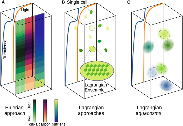
Figure 1. Schematic of different phytoplankton modeling approaches. (A) The vertical distribution of phytoplankton carbon and chlorophyll can be simulated according to vertical nutrient and light gradients and a turbulent field. The Eulerian approach samples all active fields at the nodes of a fixed grid; fine and microscale stirring (turbulence) is modeled as irreversible mixing, wiping out fine, and microscale patchiness. (B) The Lagrangian Ensemble approach bundles individual cells into Lagrangian parcels; the number of organisms per parcel is modified by infra-parcel ecological interactions; unresolved turbulence is modeled as a stochastic motion of the parcels, which don't interact with each other. (C) The Lagrangian aquacosm approach tracks tiny Lagrangian water masses (aquacosms) moving as in (B); biogeochemical interactions occur within aquacosms, which are permeable, thus allowing for mass exchanges between nearby aquacosms.

Other models use the Lagrangian formulation, which singles out either small portions of the fluid or individual biological agents, and follows them along their motion (Figure 1B). Despite their approximations (e.g., number of parcels insufficient to resolve all the fluid structures and use of stochastic processes to mimic turbulence), Lagrangian models describe stirring processes as such, rather than assimilating their effect to irreversible mixing. In plankton modeling, the Lagrangian formulation, originally identified with the term Lagrangian ensemble (Woods and Onken, 1982; Wolf and Woods, 1988; Woods et al., 1994; Woods, 2005), is often referred to as individual-based modeling (Cianelli et al., 2012). We argue that a clear distinction should be made between single cell Lagrangian models (Yamazaki and Kamykowski, 1991; Kamykowski et al., 1994), or agent-based models, in which the movement of a single individual is followed, but growth/death processes and cell division are not included, and Lagrangian ensembles (Figure 1B), where the super-individual concept (Scheffer et al., 1995) is used to describe the plankton population dynamics, falling back to a description of biogeochemical processes based on interacting concentration fields.

Some authors have stated the superiority of the Lagrangian approach in describing plankton dynamics (Woods, 2005; Hellweger and Kianirad, 2007; Hellweger and Bucci, 2009; Baudry et al., 2018), because they allow the reconstruction of the life history of individual water parcels, and thus, ideally, of individual cells, tracking how they adapt to the local environment as the fluid moves. However, there are intrinsic limitations to applying the super-individual concept to the modeling of phytoplankton communities, because a Lagrangian ensemble is not conceived to exchange with surrounding ensembles any of the active agents that it carries (Figure 1B). Therefore, nearly all Lagrangian models (but see Dippner, 1998) neglect to include irreversible mixing processes. In the sporadic cases where Lagrangian and Eulerian formulations have been compared, this issue appears to have been overlooked (Wolf and Woods, 1988; Lande and Lewis, 1989; McGillicuddy, 1995; Kida and Ito, 2017; Baudry et al., 2018), even though it may lead to unrealistic, even paradoxical outcomes.

Consider a region of ocean with steady conditions, favorable for a phytoplankton bloom. Assume an initial random distribution dividing the fluid in very small patches, half devoid of phytoplankton, and the others at carrying capacity, which is the maximum phytoplankton biomass allowed by the system at those conditions. The ensembles of a Lagrangian model would mimic these patches, but, lacking any mutual interaction, plankton in those already at carrying capacity would never reach the nearby empty ones and trigger growth. The ensembles lacking phytoplankton would remain devoid of it, and the others would stay at the carrying capacity. The bulk concentration, computed as an average over all the Lagrangian ensembles, would indefinitely remain at one half of the carrying capacity: a baffling outcome given the favorable conditions! In an Eulerian model, irreversible mixing would quickly offset from zero the concentration of the empty nodes, triggering growth, so that the bulk concentration will eventually reach the carrying capacity. However, if the initial subdivision of empty and full patches were too fine to be resolved, then the amount of irreversible mixing computed by the Eulerian model would be a gross overestimation of the real one, which begs the question whether the modeled growth rate of the bulk concentration is realistic (Baudry et al., 2018).

Turbulent stirring, irreversible mixing, and growth are each associated to their own distinct time scales. For example, the celebrated Sverdrup model (Sverdrup, 1953) for the onset of phytoplanktonic blooms stems from the assumption that the growth time scale is slower than the stirring time scale. It is of extreme historical importance, and is the founding stone that all later bloom models have confronted, either to build on it, or to overthrow it (Fischer et al., 2014; Sathyendranath et al., 2015). It also has a peculiar feature: owing to its linearity, substituting stirring with irreversible mixing (if characterized by the same time scales as the stirring) leaves the results unchanged. As we shall illustrate in the following, in the presence of non-linear biological terms, this equivalence is lost: in Sverdrup-like non-linear models, the separation between the time scales of stirring and of irreversible mixing determines the tempo and mode of the bulk phytoplankton growth. The proliferation of explanations for the occurrence of blooms, often distinct from each other by subtle details, may be a symptom of the lack of appreciation for a key theoretical issue: phytoplankton patchiness affects the bulk growth.

Occasionally, some attempts have been made to parameterize patchiness effects into Eulerian biogeochemical models. Realizing that the biological response is greatly affected by the treatment of the unresolved scales, authors like Fennel (Fennel and Neumann, 1996) have long proposed to use “effective” biological parameters. A time-delay parameterization was suggested for the case where patchiness is the result of oscillatory population dynamics occurring with different phases in different places (Wallhead et al., 2006). More recently, a closure parameterization was introduced, reminiscent of those used for turbulence (Mandal et al., 2016, 2019). Because the approach requires a truncated Taylor expansion of the non-linearities, it is formally valid only when the fluctuations are small, which high resolution chlorophyll profiles suggest is not the case (Doubell et al., 2014). Furthermore, it requires one additional equation for each pair of tracer variables, in order to track the evolution of their covariance, which may result in a substantial increase of the computational cost for some applications.

Overall, the bulk of the literature appears to overlook the issue, treating biogeochemical tracers in the same way as non-reacting ones.

We argue that the strategy of replacing unresolved transport with irreversible mixing, and then compensating the resulting biases by means of some parameterization, will face overwhelming difficulties. For example, different initial conditions, keeping everything else the same, may yield different bulk growth rates (Paparella and Popolizio, 2018) (an issue also noted in the early work on the plankton patchiness theory; Martin, 2003).

If turbulent stirring, irreversible mixing, and growth processes are modeled separately and independently from each other, then reproducing realistic phytoplankton dynamics in predictive models should become much easier. A class of Lagrangian methods recently proposed (Paparella and Popolizio, 2018) achieves this goal by depicting Lagrangian parcels as representing microscale-sized, homogeneous control volumes of water, rather than individual organisms or ensembles. In this framework, irreversible mixing processes are represented by exchanging small mass fluxes between nearby parcels. We call aquacosms such Lagrangian parcels subject to coupling fluxes (Figure 1C, section 2). The coupling is regulated by a parameter, p, whose value is proportional to the intensity of the fluxes. As we shall demonstrate, p sets the time scale associated with the irreversible destruction of biogeochemical variance at the microscales, which, in this approach, remains independent of the time scales of mechanical stirring. Results analogous to those of Lagrangian ensemble models are recovered for uncoupled parcels (p = 0). In the opposite limit, high values of p produce an excessive irreversible mixing, and yield results strongly resembling Eulerian simulations.

In the rest of the paper we shall build a hierarchy of models, from simple, idealized ones up to moderately realistic ones, to illustrate in detail the biases that Eulerian and Lagrangian ensemble models may generate in the presence of plankton patchiness, and the benefits of the aquacosm approach. Through the idealized models we identify two distinct mechanisms that generate and sustain patchiness in the biology, provided that transport and irreversible mixing are modeled as distinct processes. These findings reveal that irreversible mixing shapes the interaction between biogeochemical processes occurring at the microscales and larger scale transport processes. Building on these results, we use two simulations of an open ocean phytoplankton bloom, with parameters and forcings appropriate for the North East Pacific (PAPA station), and for the Southern Ocean sub-Antarctic Zone (SAZ), to illustrate that the same mechanisms are at work in the open ocean, affecting important parameters such as plankton patchiness, primary productivity and phenology of the bloom.

2. Methods

Here we present all of the models that we shall use in the next section. In all cases, they describe a column of fluid in turbulent motion, where the only spatial dimension is the vertical (denoted by z). The complexity of the biological reaction term is progressively augmented although kept to a minimum level to better highlight the interplay between physics and biology.

We first present the Eulerian, eddy-diffusive formulation of each model, where turbulent transport is not explicitly resolved, and is instead parameterized as an eddy diffusivity term. At the end of the section we describe the aquacosm Lagrangian formulation, which represents turbulence as a stochastic vertical transport of fluid parcels, and explicitly allows for additional irreversible mixing of tunable intensity. When the intensity of irreversible mixing is reduced to zero, one recovers a standard Lagrangian ensemble model. In the paper we will use the term aquacosm to refer to interacting Lagrangian fluid parcels as shown in Figure 1C.

2.1. Idealized Eulerian Models

We begin with a simple turbulent dispersion model with no reaction term. Assuming homogeneity throughout the water column, the Eulerian, eddy-diffusive formulation describes the flow with the following diffusion equation

$\begin{array}{ll}\frac{\partial C}{\partial t}=\frac{{\partial }^{2}C}{\partial z^2}& (1)\end{array}$

where C is the concentration of a non-reactive substance dissolved in the fluid. The model is already written in non-dimensional units [see below, before Equation (5) for details]. We impose no-flux boundary conditions at the ends of the water column 0 < z < 1. We choose as initial condition the step function

$\begin{array}{ll}C(z,0)=\{\begin{array}{ll}0,& z<1/2\\ 1,& z\ge 1/2\end{array}.& (2)\end{array}$

Next we consider a homogeneously turbulent water column carrying an idealized phytoplankton population subject to a logistic growth limited by the availability of light, whose intensity decreases as a function of depth. This is a generalization of the celebrated Sverdrup model of the onset of open-ocean blooms (Sverdrup, 1953). In dimensional units, the Eulerian, eddy-diffusive model is

$\begin{array}{ll}\frac{\partial C}{\partial t}=\kappa \frac{{\partial }^{2}C}{\partial z^2}+rf(z)C\left(1-\frac{C}{K}\right)& (3)\end{array}$

where κ is the eddy diffusivity, assumed to be constant, and r is the maximum growth rate of phytoplankton, having concentration C and carrying capacity K. Zero-flux boundary conditions are imposed at both ends of the water column, that is at z = 0 and z = ℓ. The non-dimensional function f quantifies the balance between light-stimulated growth, and loss of biomass due to respiration. Sverdrup defined it as

$\begin{array}{ll}f(z)=e^{-\lambda z}-\frac{\mu }{r},& (4)\end{array}$

where μ is a constant respiration rate, and λ is a measure of water transparency. Choosing ℓ as the unit of length, ℓ²/κ as the unit of time, and K as the unit of concentration, Equation (3) takes the non-dimensional form:

$\begin{array}{ll}\frac{\partial C}{\partial t}=\epsilon f(z)C(1-C)+\frac{{\partial }^{2}C}{\partial z^2}.& (5)\end{array}$

The parameter ε = rℓ²/κ expresses the ratio of the turbulent and of the biological time scales (the former quantified through the eddy diffusivity as ℓ²/κ). For ε ≪ 1 the linearized version of this model reduces to the Sverdrup model.

2.2. The SAZ and PAPA Eulerian Models

We simulate open-ocean phytoplankton blooms at two distinct stations, intended to represent the North East Pacific and the Atlantic sector of the Southern Ocean. The chosen station locations are representative of two typical stratification regimes in the open ocean. Since we focus on the relationship between turbulence and light, the key distinguishing feature is the time evolution of the vertical water column structure. Weather station PAPA is located in the North-East Pacific (50°N, 145°W), and is characterized by mixing confined to less than 100 m with maximum cooling in March-April and the development of summer stratification between June and October. The PAPA station has been used in the literature to develop and analyze turbulence closure models (Burchard and Bolding, 2001; Reffray et al., 2015). We use a 1-D version of the NEMO physical ocean model with the parameterizations described in Reffray et al. (2015), implementing the generic length scale turbulence closure. The model is run with 75 vertical levels extending from the surface to the ocean floor and is forced by ECMWF ERA-interim reanalyses (Dee et al., 2011), to obtain hourly values of the eddy diffusivity required by the Eulerian and Lagrangian biogeochemical models. A similar model is used for the Sub-Antarctic zone of the Southern Ocean (SAZ), with the same vertical grid and same type of atmospheric forcing as in PAPA. This model site is ideally located in the Atlantic sector at 45°S 8°E, in similar light conditions as for PAPA. This region features deep mixing beyond 100 m between May and August and weak stratification during the Austral summer months.

To move forward from the logistic growth model used as an idealized case, we adopt a more realistic but still simplified version of the Biogeochemical Flux Model (Vichi et al., 2007). The chosen formulation tracks phytoplankton carbon concentration C, measured in mg m⁻³, for a generic functional type of mid-sized diatoms, in which growth is only limited by light availability and an implicit temperature dependence is included in the parameter choice to account for the different oceanic regions.

The photosynthetic available radiation E_PAR is propagated according to the Lambert-Beer formulation

$\begin{array}{ll}{E}_{PAR}(z)={\epsilon }_{PAR}{Q}_S{e}^{{\lambda }_{w}z+{\displaystyle {\int }_z^0}{\lambda }_{bio}(z^{\prime })d{z}^{\prime }}& (6)\end{array}$

where Q_s is the net broadband solar radiation at the surface from ERA-interim (W m⁻²), ε_PAR = 0.4/0.217 is the coefficient determining the fraction of photosynthetically-available radiation (converted to μE m⁻²s⁻¹ using the constant 0.217). Light propagation takes into account the extinction due to pure water λ_w (0.0435 m⁻¹) and to phytoplankton concentration λ_bio. The broadband biological light extinction is approximated to a linear function of the phytoplankton chlorophyll concentration L

$\begin{array}{ll}{\lambda }_{bio}=cL& (7)\end{array}$

regulated by the specific absorption coefficient (c = 0.03 m² mg chl⁻¹). To be more comparable with the non-dimensional idealized experiments, the model neglects photoacclimation phenomena, therefore we assume

$\begin{array}{ll}L={\theta }_{chl}C& (8)\end{array}$

where the chlorophyll to carbon ratio θ_chl was taken to be 0.017 mg chl mg C⁻¹ for PAPA and 0.013 for SAZ (Behrenfeld et al., 2005; Thomalla et al., 2017). The same results (not shown) were confirmed using the BFM acclimation model with variable chlorophyll, based on the Geider et al. formulation (Geider et al., 1997; Vichi et al., 2007). The carbon concentration rate of change is controlled by gross primary production, respiration and a crowding mortality term that parameterizes unresolved loss terms such as zooplankton grazing:

$\begin{array}{ll}Ċ=r{f}^{E}C-bC-\frac{a{C}^2}{C_h+C}& (9)\end{array}$

where r is the maximum specific photosynthetic rate, b is the basal specific respiration rate, a is the specific crowding mortality rate and C_h is the crowding half-saturation. Owing to the difference in the seasonal cycle of nutrients and water temperature, we use r = 2, b = 0.16, a = 1 days⁻¹ for PAPA and r = 0.5, b = 0.04, a = 0.25 days⁻¹ for SAZ. The lower realized growth rate in SAZ is due to the different mean temperature during the bloom period (see Equation (7) and (16) in Vichi et al., 2007). The other parameters are tuned to yield realistic values of chlorophyll at the study sites. In all cases we set C_h = 12.5 mg m⁻³. The light regulating factor is defined as

$\begin{array}{ll}{f}^E=1-exp\left(-\frac{\alpha E_{PAR}}{r}{\theta }_{chl}\right)& (10)\end{array}$

where α = 1.3810⁻⁵ μE⁻¹m² (Vichi et al., 2007).

The eddy-diffusive Eulerian version of this model is

$\begin{array}{ll}\frac{\partial C}{\partial t}=\frac{\partial }{\partial z}\left(\kappa (z,t)\frac{\partial C}{\partial z}\right)+Ċ.& (11)\end{array}$

Starting from initial conditions having a small constant concentration, the runs extend for 4 years (each year repeats the same eddy diffusivity and radiation data). Except for the first year, in all models the results have negligible differences between the years.

2.3. Numerical Eulerian Scheme

All the Eulerian models in this paper are solved with an explicit, second-order finite differences scheme, with C and κ evaluated on staggered uniform grids. The depth of the simulated water column is one non-dimensional length unit for the idealized cases, and 200 m deep for the PAPA and SAZ simulations. In all cases the distance between consecutive grid nodes is 1/200 of the domain length. No-flux boundary conditions are imposed at the top and bottom of the water column. The eddy diffusivity κ is interpolated onto the uniform grid with the same B-spline interpolator used for the Lagrangian simulations (see below).

2.4. Lagrangian Aquacosm Simulations

A generic Lagrangian-ensemble water-column model is embodied by the following equations

$\begin{array}{ll}d{z}_i=\frac{\partial }{\partial z}\kappa (z_i,t)dt+\sqrt{2\kappa (z_i,t)}d{W}_i& (12)\end{array}$

$\begin{array}{ll}\{\begin{array}{ll}{ċ}_i^{(1)}& =f_1(c_i^{(1)},\dots ,c_i^{(m)},z_i,t)\\ & ⋮\\ {ċ}_i^{(m)}& =f_m(c_i^{(1)},\dots ,c_i^{(m)},z_i,t)\end{array}& (13)\end{array}$

where the index i = 1, …, N identifies the parcel having depth z_i, that performs a Brownian motion characterized by an eddy diffusivity κ, which may depend on depth and time t; W_i is a realization of the standard Wiener process. See Gräwe (2011) and Van Sebille et al. (2018) for a derivation of Equation (12). The quantities $c_i^{(1)},\dots ,c_i^{(m)}$ are the concentrations of the m scalar quantities describing the planktonic ecosystem (e.g., in the model of section 2.2, it would be m = 2, if we had modeled separately the dynamics of the concentration of phytoplankton carbon and chlorophyll) and the overlying dot denotes the time derivative. The functions f₁, …, f_m describe the reaction kinetics, where the dependence on depth and time accounts for the effect of light and its daily and seasonal variations, and for any other external forcing.

In the aquacosm approach we interpret the Lagrangian parcels as tiny control volumes. They should be thought of as minuscule aquatic mesocosms, which are carried by the ocean dynamics, and are homogeneous in their scalar content. This interpretation is shared with the Lagrangian-ensemble models, but, to avoid the issues discussed in the introduction, they are not isolated and exchange mass between nearby aquacosms (see Figures 1B,C). Following Paparella and Popolizio (2018), we define the mass fraction q_ij that the i−th aquacosm gives to the j−th aquacosm as

$\begin{array}{ll}{q}_{ij}=\{\begin{array}{ll}p{(4\pi K_{ij}\Delta t)}^{-1/2}exp\left(-\frac{|z_i-z_j{|}^2}{4K_{ij}\Delta t}\right),& |z_i-z_j|<R\\ 0,& |z_i-z_j|\ge R\end{array}& (14)\end{array}$

where R is an interaction radius, and the parameters p and the symmetric matrix K are defined below. At intervals of time Δt, we update the concentrations carried by each parcel as

$\begin{array}{ll}{c}_i^{(l)}\leftarrow c_i^{(l)}-{\displaystyle \sum _{j=1}^N}{q}_{ij}{c}_i^{(l)}+{\displaystyle \sum _{j=1}^N}{q}_{ji}{c}_j^{(l)},l=1,\dots ,m& (15)\end{array}$

for all the scalars l = 1, …, m. The first sum represents the mass fraction that leaves the i−th aquacosm and is redistributed to all the other aquacosms, and the second sum, conversely, represents an equal mass fraction received by the i−th aquacosm from all the others (note that q_ij = q_ji). The received mass fraction is composed of many distinct parts, each carrying the concentration of the scalars contained in the acquacosm of provenance. These parts immediately and irreversibly homogenize with the remaining content of the i−th aquacosm in order to determine its new concentration values. The constant p is a free parameter, which in this one-dimensional formulation has the dimensions of a length, but in three dimensions would be a volume, that can be used to tune the coupling strength between the aquacosms (choosing p = 0 is equivalent to isolating the parcels as in a Lagrangian ensemble model). The variance K_ij of the Gaussian kernel coupling the i−th and j−th aquacosms is chosen on the basis of the eddy diffusion coefficient as

$\begin{array}{ll}{K}_{ij}=min\left\{\kappa (z_i,t),\kappa (z_j,t)\right\}.& (16)\end{array}$

The choice of the minimum is dictated by the observation that there is very little flux across a region where the eddy diffusivity jumps from very small to very high values, e.g., at the base of the mixed layer. In order to allow for an efficient numerical implementation, the coupling between aquacosms further apart than the interaction radius R must be zero. This algorithm conserves mass and avoids the creation of spurious maxima and minima (Paparella and Popolizio, 2018), provided that the parameters are chosen so that, for all i = 1, …, N, it is

$\begin{array}{ll}{\displaystyle \sum _{j=1}^N}{q}_{ij}\le 1.& (17)\end{array}$

Roughly speaking, one may think the aquacosms as oozing out part of their content into Gaussian clouds spreading at a rate specified by the eddy diffusion coefficient (Figure 1C). Then, at regular intervals of time Δt, all the material within a control volume (both what was left inside the volume, and what came from the overlapping clouds) is instantaneously and irreversibly homogenized, thus determining the concentrations which will evolve according to (13) for the next interval of time Δt. A conceptually similar technique describing advection-diffusion processes as the interleaving of short time intervals of pure transport alternated with instantaneous irreversible mixing events has already been successfully used to model mixed layer dynamics (Ferrari and Young, 1997). These sort of modeling procedures have their justification rooted in the fractional step method for the numerical solution of differential equations. From a different point of view, we should note the similarity between the aquacosm approach and the so-called tanks-in-series model, popular in chemical and environmental engineering (see e.g., Levenspiel, 2011, Chapter 8). The main difference is that, in that case, the topology of the interconnections between tanks does not change in time, while here the existence of a flux connecting two aquacosms depends on their relative position.

All Lagrangian results presented in this paper use 200 aquacosms. Equations (12) and (13) were integrated using, respectively, Milstein's and the midpoint methods (Gräwe, 2011; Van Sebille et al., 2018), with a time step Δt = 10⁻⁵ non-dimensional time units for the idealized cases of Figures 2–4 and Δt = 5 s for the PAPA and SAZ cases. The eddy diffusivity κ used in Equations (12) and (16) is the same as that of the corresponding Eulerian model. In particular, the eddy diffusivity for the PAPA and SAZ simulations are generated by the NEMO ocean model as described in section 2.2, and are interpolated at the position of the aquacosms with monotone B-splines (Ross and Sharples, 2004). In these two simulations the reaction terms (13) reduce to (9). Reflecting boundary conditions are imposed at both ends of the water column on all Lagrangian simulations. The interaction radius in Equation (14) is R = 0.05 non-dimensional units for the idealized cases and R = 10 m for the PAPA and SAZ simulations.

FIGURE 2

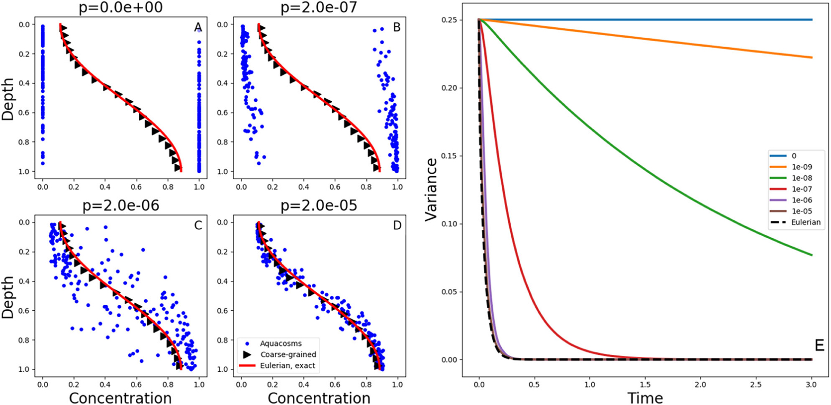
Figure 2. (A–D) Exact solutions at time t = 0.05 of the diffusion Equation (1) with the initial condition (2) and no-flux boundary conditions (red lines). The blue dots show the position and the concentration of the aquacosm simulations with the same diffusivity and varying coupling strength p. The black triangles are a coarse-grained version of the same data, obtained with a Gaussian kernel estimator with standard deviation 0.1 (see section 2). (E) variance, as a function of time, in Lagrangian aquacosm simulations with varying coupling strength p (solid lines) and variance of the exact solution of the Eulerian problem (1) (dashed line).

FIGURE 3

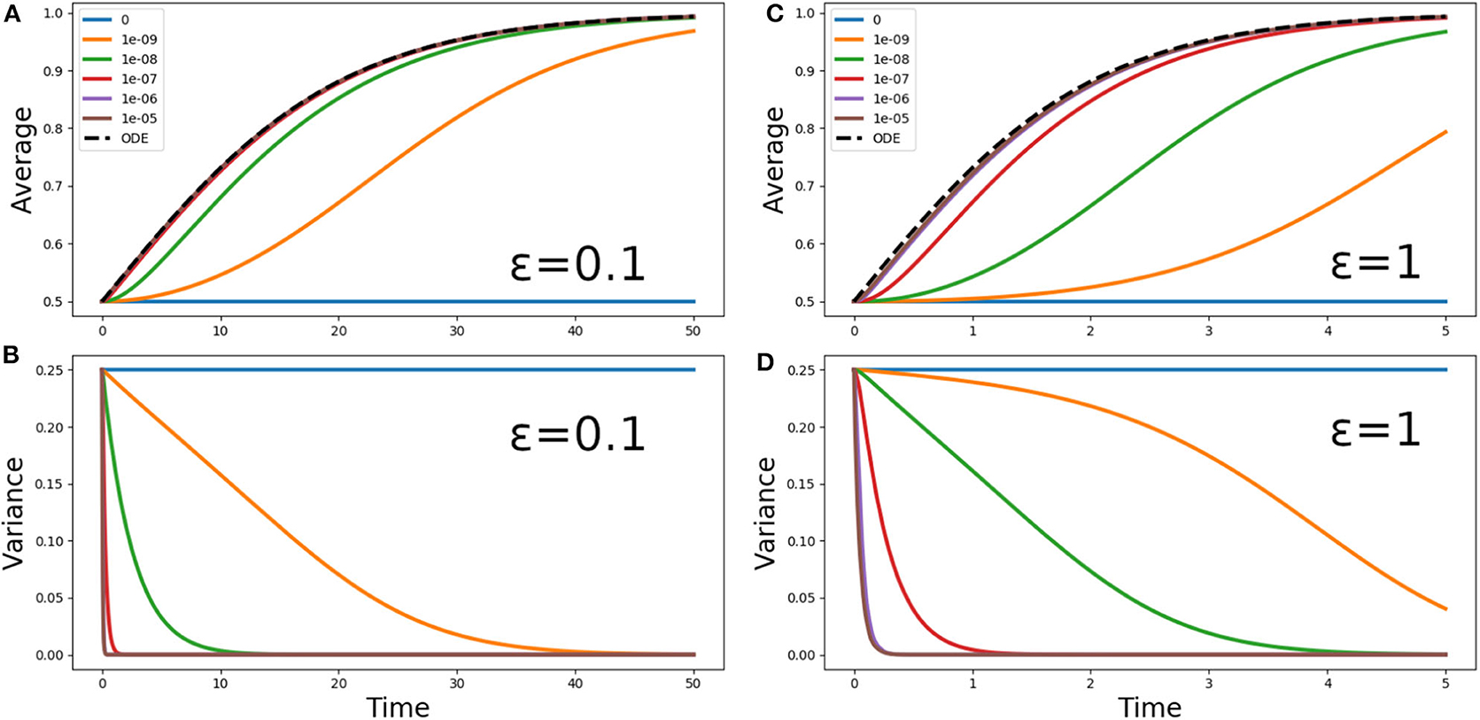
Figure 3. (A,C) Average phytoplankton concentration and (B,D) variance, as a function of time, for the problem (5) with f(z) = 1, ε = 0.1 (A,B) or ε = 1 (C,D) and the step initial condition (2). The solid lines refer to Lagrangian aquacosm simulations with varying strength of the coupling parameter p. The dashed line is the solution of the Sverdrup's approximation (18). Note the different ranges of the time axes.

FIGURE 4

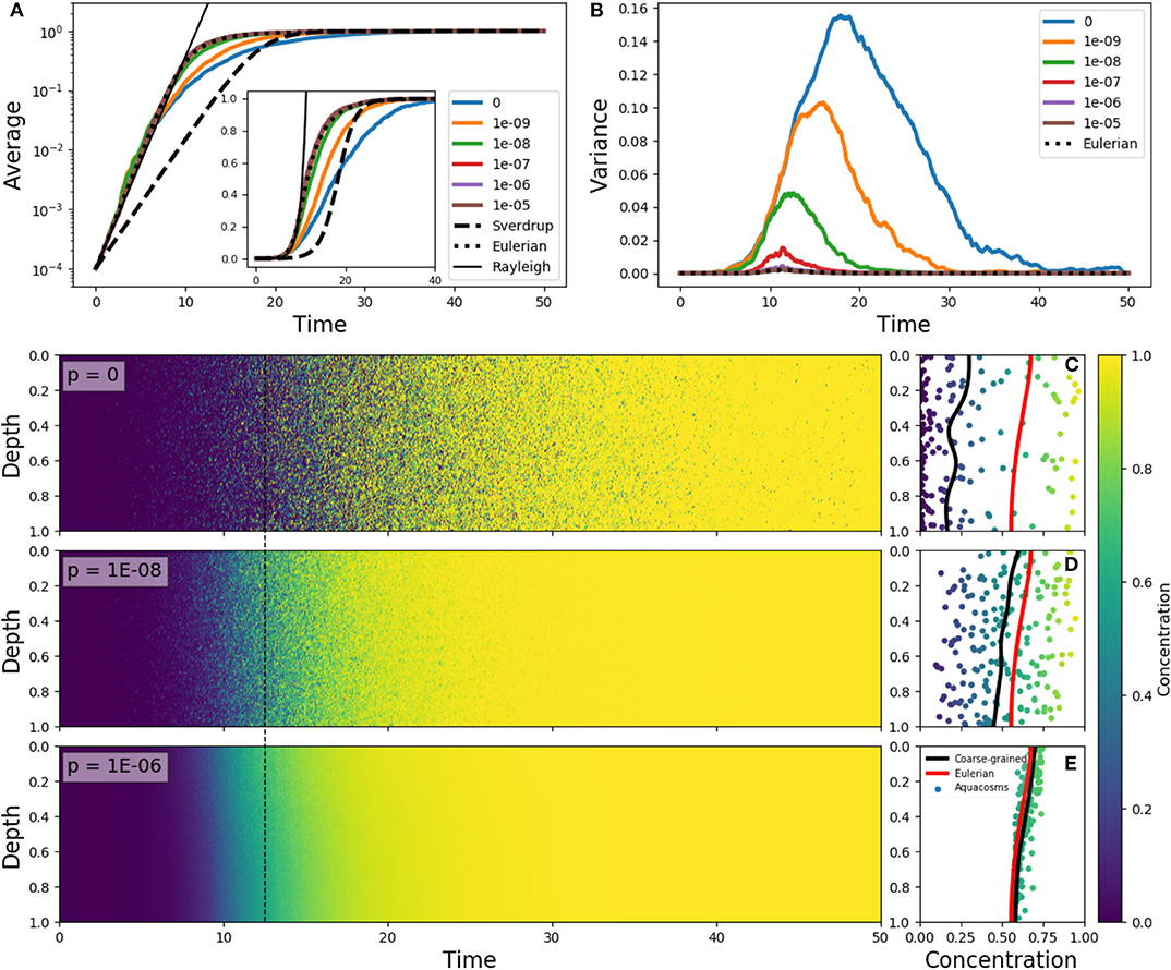
Figure 4. (A) Average phytoplankton concentration and (B) variance as a function of time, for the Eulerian problem (5) with f(z) = e^−z/0.15 − 0.1, ε = 10 and constant-in-space initial condition C(z) = 10⁻⁴ (dotted lines). The solid lines in color refer to Lagrangian aquacosm simulations with the same parameters, with varying coupling strength p. The dashed line is the solution of Sverdrup's approximation (18). The thin black line is an exponential growth with a rate estimated by means of the Rayleigh quotient (section S2 in Supplementary Material) associated to Equation (5). The inset shows the same data as (A) but with a linear, rather than logarithmic, vertical axis. (Lower panels) Plankton concentration as a function of depth and time for Lagrangian simulations with p = 0, 10⁻⁸, 10⁻⁶. (C–E) concentration and depth of the aquacosms (dots), coarse-grained concentration of the aquacosms (black line) and numerical solution of the Eulerian model (red line) at the time marked by the dashed black line in the left panels.

In the following, the amount of patchiness present in the various models is evaluated and visualized by showing the fluctuations around local averages, which we call coarse-grained profiles, and are obtained by smoothing the concentrations with a Gaussian kernel estimator (Gräwe, 2011) having a standard deviation of 1/20 of the domain for the idealized cases and 2.5 m for PAPA and SAZ, or as otherwise specified in the figure caption. As it is customary for fields transported by turbulence, we also quantify such fluctuations by evaluating the variance of the concentration field (see e.g., Warhaft, 2000 for more details). In the Eulerian formulation the variance is defined as 〈(C − 〈C〉)²〉, where the angular brackets denote an average over the whole water column. In Lagrangian models, the variance of the concentration field is estimated just by computing the variance of the concentration values carried by each parcel.

3. Results

3.1. Pure Stirring and Mixing

First, we shall consider the case of turbulent stirring and mixing of a substance not subject to any reaction (section 2.1). The Eulerian formulation of this problem is given by Equation (1). The aquacosm formulation uses κ = 1 in Equations (12) and (16), and no reaction terms.

Figures 2A–D show the concentration and position of the aquacosms for different values of the coupling parameter p, together with the analytical solution of Equation (1). The Brownian motion scrambles the order of fluid parcels initially arranged as to produce the step-like initial condition (2), and this produces patchiness: a random alternation of parcels with high and low concentration values. Irreversible mixing equalizes the concentration of nearby parcels, thus removing patchiness, more and more effectively as the coupling strength p increases. Local weighted averages of the Lagrangian result (black triangles, see section 2), are essentially identical to the analytic solution of the Eulerian model. This coincidence might suggest that the Eulerian and all of the Lagrangian models are equivalent. The coarse-graining process of taking local averages, however, gives only a partial picture. Figures 2A–D do not depict equivalent microphysics. The concentration carried by the individual parcels (which, ultimately, is all that matters for the reaction terms when they are present) is vastly different in the four cases. The amount of irreversible mixing, set by the parameter p, determines how quickly the fluctuations around the local averages are dissipated, that is, p sets the time scale associated to irreversible mixing processes. We note that, on rearranging the position of the parcels without changing their concentration, the variance shown in Figure 2E remains the same (variance is invariant with respect to permutations). Therefore, in the special case p = 0, that is, when aquacosms are uncoupled and each maintains its initial concentration, the variance remains constant in time, and equal to the variance of the initial condition, even though the local averages still tend to uniformity, as prescribed by (1). The reason is that the Brownian motion (or the turbulent stirring in an actual turbulent water column) eventually produces such a fine interleaving of nearby parcels with vastly different concentrations, that upon averaging those fluctuations cancel out (Figure 2A). When p > 0 then the irreversible mixing [in the present model represented by mass exchanges between nearby aquacosms as in Equations (14) and (15)] damps the difference in concentration between nearby regions of the fluid, and thus reduces the variance, which becomes a decreasing function of time (Figure 2E). As the amount of irreversible mixing increases (that is, for increasing values of p) the decrease of fluctuations, and thus of the variance, becomes quicker. For sufficiently large values of p the variance decays just as quickly as in the Eulerian, eddy-diffusive case, where stirring is all assimilated to irreversible mixing.

3.2. Sverdrup's Model Expanded

3.2.1. Fast Turbulence, Homogeneous Light

Next we shall consider Equation (5), which is a very simple model of light-limited growth. If the time scale of turbulent overturning is much faster than the time scale of biological growth, that is for ε ≪ 1, following Sverdrup (Sverdrup, 1953), one can argue that physics and biology disentangle: first turbulence makes the initial condition vertically homogeneous, in a coarse-grained sense, within a transient no longer than O(1), and keeps the concentration C independent of depth at all later times. Then, on O(ε⁻¹) time scales, the vertically constant concentration changes in time according to the ODE

$\begin{array}{ll}Ċ=\epsilon IC(1-C)& (18)\end{array}$

where I is the integral over the water column of the function f that appears in Equation (5) (see Supplementary Material S1), and the dot denotes a derivative with respect to time. Sverdrup's approximation does not require a specific form of the function f, but holds for any integrable f sandwiched between O(1) bounds. The comparison with eddy-diffusive, Eulerian numerical simulations shows that in practice this approximation gives good results up to ε ≈ 1.

The aquacosm formulation of this problem uses κ = 1 in Equations (12) and (16). The only reaction term in Equation (13) coincides with the reaction term of Equation (5).

As it should be clear from the previous subsection, reaching coarse-grained homogeneity implies having reached homogeneity at all scales in an eddy-diffusive Eulerian model, but not necessarily in a Lagrangian one (nor in the real world). This discrepancy leads to question the equivalence of the eddy-diffusive Eulerian and of the Lagrangian formulations (Lande and Lewis, 1989; McGillicuddy, 1995). We show here, and demonstrate analytically in section S1 of the Supplementary Materials, that for the linear Sverdrup model the two approaches yield the same averages, but non-linear reaction terms break down the equivalence.

Figure 3 shows the phytoplankton concentration mean and variance as a function of time for Equation (5) and its aquacosm counterpart, with f(z) = 1, the initial condition (2), and two values of the ratio ε = 0.1 and ε = 1. As sketched in the introduction, because all fluid parcels are initially set at a fixed point of the reaction terms (namely, half of them at C = 0 and the other half at C = 1, the value of the carrying capacity), with uncoupled aquacosms (p = 0) the mean unrealistically remains at one half of the carrying capacity despite the positive growth rate. When the coupling between the aquacosms is switched on, the mean gradually tends to the carrying capacity (C = 1) and the variance tends to zero. The rapidity with which the asymptotic values are approached depends on the strength of the coupling parameter p: high values produce results that behave just as predicted by Sverdrup's theory, but small ones produce growth curves that are nothing like the solution of the ODE associated with the reaction term.

3.2.2. Slow Turbulence, Inhomogeneous Light

The examples so far show that the fast stirring of a step-like initial condition produces patchiness, which then affects the bulk growth rate. Much attention has been given to the case of non-homogeneous biological growth [e.g., using the form (4) for f(z)] when growth is faster than stirring. Then, according to the critical turbulence theory (Huisman et al., 1999; Taylor and Ferrari, 2011; Ferrari et al., 2015), phytoplankton closer to the surface contributes to the overall growth more than Sverdrup's theory would provide for, so that a bloom may initiate even when the average light would not allow for that. Differences in light history and acclimation have also been affirmed to produce growth when Sverdrup's theory would predict decay (Lande and Lewis, 1989; Woods et al., 1994; Esposito et al., 2009). What has not been stressed is that these conditions would also naturally lead to the creation of patchiness if irreversible mixing processes are not fast enough to remove it. When growth is faster than turbulent stirring, then the phytoplankton in water parcels at shallow depth will have time to grow substantially more than that in the deeper parcels spending some time in darkness. As stirring makes some of the shallow parcels sink and replaces them with some of those that were at depth, then microscale patchiness ensues. Just as in the case of a step-like initial condition, patchiness affects growth. As the bloom progresses, water parcels having spent the most time close to the surface reach the carrying capacity before the others, and the rapidity of the bulk growth becomes regulated by the intensity of the irreversible mixing, which transfers the phytoplankton from high to low concentration parcels.

This process is illustrated in Figure 4 for different degrees of the coupling between aquacosms. In the initial linear regime, when phytoplankton concentration is much smaller than the carrying capacity, the Eulerian model (5) and all the Lagrangian models show the same growth rate of the bulk concentration (Figure 4A), which is in excess of what Sverdrup's theory would dictate. This is in agreement with the critical turbulence prescriptions as long as the process is linear (see section S2 of Supplementary Materials for a demonstration). In the non-linear regime, the Lagrangian models yield distinct results: with small coupling strength, variance grows with time (Figure 4B), and this leads to bulk growth significantly slower than in the eddy-diffusive Eulerian model, due to the patchy environment. Once again, destroying the variance by using a strong enough coupling parameter recovers the results of the Eulerian model. Figures 4C–E shows that variance genuinely corresponds to patchiness: with low p, aquacosms of starkly different concentration are found next to each other, and the coarse-grained equivalence of Lagrangian and Eulerian models is lost. Depending on the degree of irreversible mixing, the non-linear reaction terms lead to small-scale patchiness and substantially different time evolution of the mean phytoplankton concentration in a vertically non-uniform, slow turbulence environment.

3.3. Microscales and Phytoplankton Phenology

To demonstrate in a realistic setting how phytoplankton growth and phenology are affected by patchiness arising from the mechanisms identified in sections 3.2.1 and 3.2.2, we run the PAPA and SAZ models defined in section 2.2, using both the eddy-diffusive Eulerian and the aquacosm Lagrangian formulations.

Figure 5 shows the simulated average chlorophyll content at PAPA station over the first 50 m of water column in the weeks when the bloom starts. We define the onset of the bloom as the first day of the year when the chlorophyll content exceeds the median plus 5% of the daily chlorophyll concentration tracked over 1 year (Racault et al., 2012). Reductions of the coupling strength p delay the onset by over 2 weeks. The results diverge from each other before the onset of stratification, from mid April until the beginning of May, when the mixed layer depth is ℓ ≈ 100 m (Figure S1) and the typical mixed layer eddy diffusivity is κ ≈ 0.05 m²s⁻¹, yielding a value of ε ≈ 5 with the growth rate r = 2 days⁻¹. This suggests that we are witnessing the same process illustrated in Figure 4, where slow turbulence, a vertical light gradient, and low irreversible mixing lead to the formation of high microscale patchiness, reducing bulk growth and delaying the bloom. The Lagrangian model without any coupling (p = 0) shows the slowest growth, but this limit case is unrealistic, as demonstrated above. In the following 15 days the mixed layer becomes much shallower (Figure S1), with typical eddy diffusivity values of κ ≈ 0.025 m²s⁻¹. The time scales of growth and stirring become comparable, and the vertical light gradient ceases to be a source of patchiness. Only the entrainment of phytoplankton-poor aquacosms at the base of the mixed layer continues to be a source of patchiness. Overall, the chlorophyll content averaged over the month of the bloom initiation changes by as much as a factor 6 depending on the coupling strengths (inset B in Figure 5).

FIGURE 5

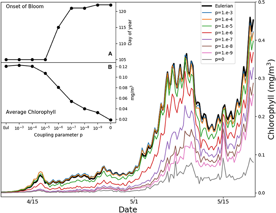
Figure 5. Average chlorophyll in the first 50 m of water column for the simulated Ocean Station PAPA in the North-West Pacific. Thin colored lines refer to aquacosm simulations coupled with varying strength p. The thick back line refers to the eddy-diffusive Eulerian model. Inset (A) shows the day of the onset of the bloom (see main text); inset (B) shows the average chlorophyll in the period April 15th to May 15th, both of them plotted as functions of the coupling parameter.

Next, we simulate the open ocean of the sub-Antarctic zone (SAZ), characterized by a mixed layer deeper than 100 m from July to October (Figure S2). Throughout the year, typical simulated eddy diffusivity values in the mixed layer are κ ≈ 0.06 m²s⁻¹, corresponding to ε ≈ 1. Here, growth is never faster than stirring, and Sverdrup's approximation holds. Therefore, only the intermittent deepening of the mixed layer, which scoops phytoplankton-free aquacosms from the depths, contributes to the creation of patchiness in the mixed layer. In the days immediately after a sudden deepening of the mixed layer, the dynamics is reminiscent of that shown in Figures 2, 3, whereby a step-like initial condition first breaks down into patchiness and then is brought to vertical homogeneity with a speed determined by the intensity of the irreversible mixing. The smaller is the mixing, the slower is the destruction of variance, and the slower is the bulk growth of phytoplankton (Figure S2). The phenological and productivity differences are not as marked as in the PAPA simulations, but we note that coarser resolution climate models with a larger impact of irreversible mixing are likely to generate greater differences and discrepancies in the bloom phenology (Hague and Vichi, 2018).

3.3.1. Comparison With BGC-Argo Float Observations

Recent bio-optical measurements using BGC-Argo floats from sub Antarctic zones (Carranza et al., 2018) reported the presence of substantial chlorophyll variance within the hydrographic mixed layer. This was interpreted as the signature of vertical gradients of chlorophyll at the fine scales (tens of meters), which called for some mechanism incompatible with the presence of strong turbulence. In particular, it was argued that periods of storm quiescence associated with slacking turbulence would occasionally leave the mixed layer homogeneous in density, but stirred only in its uppermost part, thus allowing for light-modulated growth below the turbocline (the base of the uppermost layer), generating a vertical gradient of chlorophyll.

In our models, slacking turbulence and vertical gradients of light definitely produce vertical gradients of chlorophyll, even when stirring is modeled as irreversible mixing (see e.g., the Eulerian simulation profiles in mid April and end of May in Figure S1), and effects which our models neglect, such as light-dependent grazing, may greatly enhance these gradients (Moeller et al., 2019). However, in the models where irreversible mixing is weak, patchiness, rather than these vertical gradients, is the dominant source of variance in the mixed layer. Patchiness is visually evident in the bottom panels of Figure 6. At lower values of p, very large relative differences in the chlorophyll content of nearby aquacosms are normal even above the turbocline. This extreme variability is quantified in Figure 7A (see Figure S3A for the PAPA simulations), showing the monthly average of the coefficient of variation of chlorophyll (ratio of the standard deviation and the mean) computed above the turbocline depth, thus excluding the effects of slacking turbulence. In simulations with moderate and low irreversible mixing, the coefficient of variation is never negligibly small, and even when the mixed layer is deepest and the turbulence is strongest, it doesn't drop below about 0.5. As expected, the variability is larger during the Austral summer months, when turbulence is weaker than in other seasons, showing an extended peak from spring to autumn, in full agreement with the variability observed through autonomous observations in the SAZ (Little et al., 2018). In the Eulerian simulation, and in Lagrangian simulations with very strong irreversible mixing, the peak is small and occurs in December, when the mixed layer is the shallowest, while the coefficient of variation remains negligibly different from zero in other months.

FIGURE 6

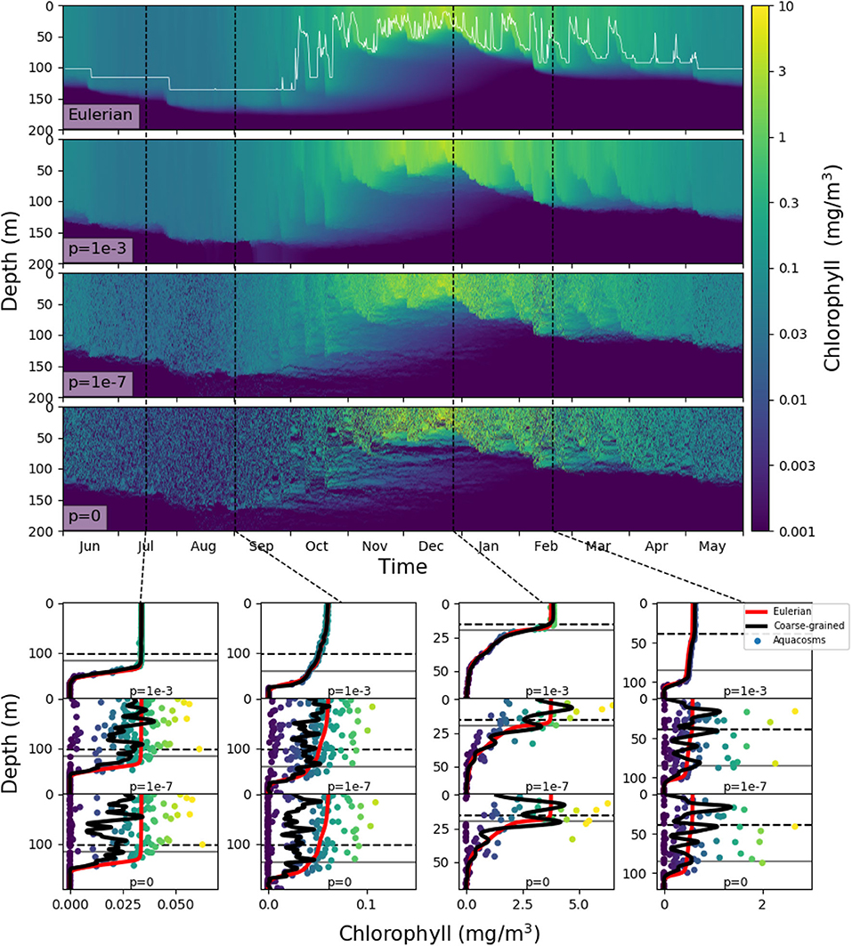
Figure 6. Top four panels: chlorophyll in the SAZ simulation in logarithmic units. The top panel shows the eddy-diffusive Eulerian model, and the thin white line marks the mixed layer depth; the next three show the aquacosm simulations for p = 10⁻³, 10⁻⁷, 0. The lower panels show, as a function of depth, the chlorophyll content in mg/m³ of the aquacosms (dots) for different values of p, their coarse-grained version (black line, see section 2), the mixed layer depth (horizontal gray line) and the turbocline depth (horizontal black dashed line) at the date marked in the upper panels by the vertical black dashed lines. For comparison, the chlorophyll concentration as a function of depth computed with the Eulerian simulation (red line) is repeated in all the panels corresponding to the same date.

FIGURE 7

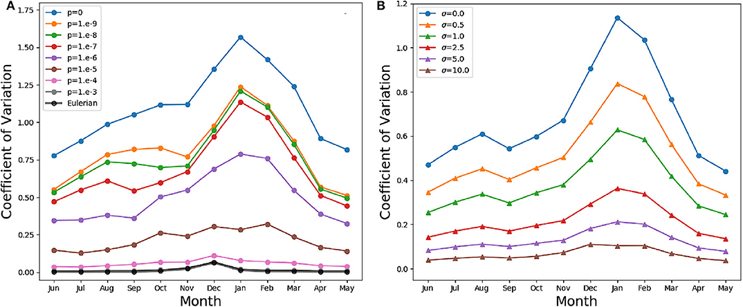
Figure 7. (A) Monthly average coefficient of variation (standard deviation over mean) of the chlorophyll above the turbocline depth in the SAZ simulation. A value of 0 indicates homogeneity, while a value of 1 implies departures from the vertical mean that are as large as the mean itself. The thin lines in color refer to the Lagrangian aquacosms with different values of the coupling parameter p. The thick black line refers to the eddy-diffusive Eulerian simulation. (B) Monthly average coefficient of variation of the Lagrangian simulation with p = 10⁻⁷, and the same quantity computed from profiles coarse-grained using a Gaussian kernel estimator with standard deviation σ = 0.5, 1, 2.5, 5, 10 m. The line σ = 0 refers to the results without coarsening.

These results, for p = 10⁻⁶ or lower, bear a strong resemblance to the statistics of the BGC-Argo float observations in the Southern Ocean (Figure 6 in Carranza et al., 2018), but suggest that, rather than by external forcing, chlorophyll variability is mostly caused by differences in the Lagrangian histories of water parcels (Kida and Ito, 2017; Baudry et al., 2018) but modulated by irreversible mixing. We remark that BGC-Argo floats are not high-resolution chlorophyll profilers (Carranza et al., 2018), and can't accurately represent vertical fluctuations on scales smaller than a few meters. The black lines in the lower panels of Figure 6 have been computed from the aquacosm concentration using a smoothing procedure yielding 5 m of resolution (see section 2), thus comparable with that of the floats. Chlorophyll fluctuations are damped, but not completely wiped out. The resolution length scale of observations affects variance estimations, as found when high-frequency sampling instruments are used (Little et al., 2018). In Figure 7B (Figure S3B for PAPA) we show the monthly average of the coefficient of variation of the simulation data relative to p = 10⁻⁷, after they underwent this coarse-graining procedure at several resolutions. Extreme smoothing yields estimates of fluctuations not far from those of the Eulerian simulations, which progressively increase as the resolution increases. Thus, albeit the BGC-Argo data are surprising in the amount of variability that they show, we suspect that this is still an underestimation of the reality.

4. Discussion and Conclusion

When considering mesoscale, and, more recently, submesoscale dynamics, it has often been stressed that the joint effect of turbulent stirring and non-linear biochemical processes must produce an uneven, patchy distribution of active tracers, and this, in turn, may affect the bulk productivity and structure of oceanic ecosystems (see Martin, 2003; Levy and Martin, 2013; Mahadevan, 2016; Lévy et al., 2018 and references therein). Here we remark that the fundamental idea expressed in those studies should also be scrutinized at smaller scales, e.g., across the water column.

We do so by contrasting the results obtained with the eddy-diffusive, Eulerian formulation and the aquacosm Lagrangian formulation for water-column models of increasing physical and biological complexity. We demonstrate in sections 3.2 and 3.3 that, in the presence of non-linear reaction terms, a discrepancy between the Lagrangian and the Eulerian formulations arises because the latter postulates the equivalence of stirring and irreversible mixing, wrongly implying that the time scales of these two processes are the same. As a consequence, a water parcel devoid of plankton and one full of plankton would equalize their concentration within the stirring time scale. When stirring and mixing are treated as separate processes, with the second allowed to be slower than the first, parcels lacking plankton are constantly seeded by the full ones, and the overall rate of growth is determined by a delicate interplay of biological processes, turbulent stirring and irreversible mixing. These findings lead to an important conclusion: in a generic non-homogeneous environment with concurrent stirring, mixing and growing, there is no reason to expect that the bulk phytoplankton concentration is described solely by the ODE associated with the reaction terms.

In order to illustrate how this delicate interplay occurs in a realistic situation, we focused on the specific problem of the onset of open-ocean blooms. There exists a very large body of literature on this decades-old subject. Some of this literature tackles the problem of how different turbulence properties affect biological growth. Yet the distinction between the time scales of turbulent stirring and the time scales of irreversible mixing is never considered. In spite of mounting evidence of ubiquitous presence of patchiness in the vertical direction across the mixed layer (Currie and Roff, 2006; Doubell et al., 2009, 2014; Foloni-Neto et al., 2016), theories of the onset of the bloom freely interchange turbulent stirring and irreversible mixing as if they were one and the same thing (see the recent review Fischer et al., 2014 and references therein). On the other hand, most of the literature on mixed layer plankton patchiness (Huisman et al., 2006; Durham and Stocker, 2011; Cullen, 2015; Moeller et al., 2019) focuses on unveiling the underlying mechanisms but does not investigate how patchiness contributes to signal at larger scales and how it should be included in predictive models.

In the present work we identified two simple and distinct mechanisms that create patchiness vertically in the mixed layer. The first mechanism, and the dominant one at SAZ, is essentially physical: when deeper, phytoplankton-poor water is entrained by turbulence into the phytoplankton-rich mixed layer, rapid mechanical stirring produces a highly patchy water column. The second mechanism requires the existence of a depth-dependent growth/decay process (e.g., due to the vertical gradient of light) acting on time scales faster than the stirring time scales. When this occurs, such as during spring at PAPA, the uneven growth at different depths creates a vertical gradient of the active tracers, which breaks down into patchiness under the action of stirring.

Eulerian models that replace unresolved stirring with irreversible mixing can't generate any patchiness from either of these mechanisms. Lagrangian ensemble models produce patchiness through both mechanisms, but their inability to represent irreversible mixing processes may lead to paradoxical results. Our aquacosm modeling framework extends the Lagrangian approach and incorporates irreversible mixing by allowing for locally interacting parcels.

The aquacosm approach appears to be preferable because, by design, the reaction terms are representative of the biogeochemical dynamics occurring in a very small, homogeneous water mass, therefore, they can effectively include empirical reaction norms derived from laboratory experiments and can retain the relationship with the environmental drivers as they were originally measured (Boyd et al., 2018). In contrast, the biological rates present in Eulerian models should always be considered as “effective” values, representative of aggregate bulk dynamics, which is not immediately comparable with laboratory experiments, or in-situ samplings.

Obviously, our PAPA and SAZ simulations should not be taken as an operational model for those two stations. In order to allow for a direct, quantitative comparison with the observed data throughout the year, the biological formulation should be expanded to include grazing, nutrients, remineralization, and, possibly, multiple phytoplankton functional groups, as well as data assimilation and formal, station-specific, parameter optimization procedures (Friedrichs et al., 2007). A comparison between Figure 5 and Figure S2 and the satellite observation of surface chlorophyll at the corresponding locations (Figure S4, data from the Ocean Colour Climate Change Initiative dataset, Version 3.1, European Space Agency) shows that at PAPA all simulations catch the May-June growth burst, but the eddy-diffusive Eulerian model has a prominent early May onset of the bloom, and that at SAZ all simulations show an early growth with respect to the December peak, but those with high irreversible mixing more so than the others.

We should stress that most Earth-System models simulate open-ocean blooms occurring earlier than the observed ones (Hague and Vichi, 2018). For strengths of irreversible mixing that we consider realistic, we find a shift forward in the onset of the bloom (section 3.2) by an amount which would largely mitigate the problem. This stubborn bias, which is the same magnitude as the projected change in bloom onset due to climate change in the twenty-first century (Henson et al., 2018), has often been attributed to inadequacies of the physical or biological formulations (McKiver et al., 2015), but in the light of our results, it is likely to stem from mismodeling the interaction, across vastly different scales, of growth and stirring, mediated by irreversible mixing.

A second puzzling issue that our findings help to unravel is that of the chlorophyll variance observed by BGC-Argo floats in the southern oceans. The proposed mechanisms for generating vertical plankton inhomogeneity in the mixed layer (referred to above) require periods of moderate to no turbulence as they occur in seasonally stratified systems like the Northeast Pacific, and thus are unlikely to be dominant in the Southern Ocean. And yet BGC-Argo floats ubiquitously find high chlorophyll variance (Carranza et al., 2018). As we showed with Figure 7, and discussed in detail in section 3.3.1, if the irreversible mixing terms are not blown out of proportion, this high variance is readily reproduced in our aquacosm framework, even though we adopt an extremely simplified description of the biological processes. This interpretation of BGC-Argo data is further corroborated by the uncanny resemblance between the distribution of chlorophyll carried by the aquacosms shown in the lower panels of Figure 6 an Figure S1 and that of the high-resolution profiles shown in Mandal et al. (2019), Doubell et al. (2014), and Doubell et al. (2009).

In this study we have used the parameter p that determines the strength of irreversible mixing as a free parameter. We have shown that for high enough values of p our aquacosm models reproduce the results of the corresponding eddy-diffusive, Eulerian model. We have also given proof that the Lagrangian ensemble models that one obtains by setting p = 0 may yield paradoxical results. For very low, but non-zero values of p, the aquacosm models appear to shed light on the problems of the bloom onset timing, and of the observed chlorophyll variance. This suggests that those low values might be physically correct, although this alone would not be sufficient for upholding such a conclusion. In the Supplementary Material S3, we develop a theoretical argument supporting it. In summary, we evaluate the mixing rule embodied by Equation (15) for a regular arrangement of aquacosms, which allows the computation of a simple formula associating p and other parameters (inter-parcel distance, time step, etc.) to a diffusion coefficient representative of the irreversible mixing processes. On identifying those processes with molecular diffusion we can match that diffusion coefficient with the known diffusivity of sea-water solutes. We find that for the simulations of section 3.3, a value of p in the range between 10⁻⁷ and 10⁻⁸ appears to be the most realistic. Obviously, the mixing processes deemed to be “irreversible” need not always be identified with molecular diffusion. For some applications other choices might be justifiable, but for modeling the mixed layer, given the recent observations of chlorophyll fluctuations below the centimeter scale mentioned in the introduction, that seems to be the most appropriate and least arbitrary choice. Because aquacosms are assumed to be homogeneous parcels of water, the identification with molecular diffusion clarifies that the size of an aquacosm should be taken as comparable with Batchelor's scale, which is the scale where the concentration of sea-water solutes is homogeneous, and which is usually no larger than a millimeter (Thorpe, 2005).

Finally, we remark that aquacosm simulations offer an ideal tool for exploring which biological features and the relative parameterizations are able to build up large-scale impacts, and which are negligible in terms of bulk properties. The aquacosm approach is not limited to the extremely simplified treatment of the growth/decay processes that we have used here to illustrate the potentialities of the method, and can be expanded to include an extreme variety of biogeochemical processes that may be deemed relevant for the specific problem at hand.

Data Availability Statement

The datasets generated for this study are available on request to the corresponding author.

Author Contributions

FP and MV ideated the aquacosm approach and wrote the paper. FP developed the aquacosm mathematical theory and wrote the water column codes. MV run the NEMO model and generated the turbulence profiles for the PAPA and SAZ simulations. All authors contributed to the article and approved the submitted version.

Funding

This research was funded by internal resources of New York University Abu Dhabi, the Center on Stability, Instability and Turbulence, MV received funding from the NRF through the South African National Antarctic Program.

Conflict of Interest

The authors declare that the research was conducted in the absence of any commercial or financial relationships that could be construed as a potential conflict of interest.

Acknowledgments

An earlier version of this manuscript was released as a Pre- Print at https://arxiv.org/abs/1909.04334. We thank the editor and the reviewers for their careful reading and thoughtful comments which greatly improved the clarity of our manuscript. The authors acknowledge the public availability of the NEMO (https://www.nemo-ocean.eu) and BFM (https://www.bfm-community.eu) models.

Supplementary Material

The Supplementary Material for this article can be found online at: https://www.frontiersin.org/articles/10.3389/fmars.2020.00654/full#supplementary-material

References

Aumont, O., Ethé, C., Tagliabue, A., Bopp, L., and Gehlen, M. (2015). PISCES-v2: an ocean biogeochemical model for carbon and ecosystem studies. Geosci. Model Dev. 8, 2465–2513. doi: 10.5194/gmd-8-2465-2015

CrossRef Full Text | Google Scholar

Azam, F., and Worden, A. Z. (2004). Microbes, molecules, and marine ecosystems. Science 303, 1622–1624. doi: 10.1126/science.1093892

PubMed Abstract | CrossRef Full Text | Google Scholar

Baudry, J., Dumont, D., and Schloss, I. R. (2018). Turbulent mixing and phytoplankton life history: a Lagrangian versus Eulerian model comparison. Mar. Ecol. Prog. Ser. 600, 55–70. doi: 10.3354/meps12634

CrossRef Full Text | Google Scholar

Behrenfeld, M. J., Boss, E., Siegel, D. A., and Shea, D. M. (2005).Carbon-based ocean productivity and phytoplankton physiology from space. Global Biogeochem. Cycles 19:GB1006. doi: 10.1029/2004GB002299

CrossRef Full Text

Bopp, L., Resplandy, L., Orr, J. C., Doney, S. C., Dunne, J. P., Gehlen, M., et al. (2013). Multiple stressors of ocean ecosystems in the 21st century: projections with CMIP5 models. Biogeosciences 10, 6225–6245. doi: 10.5194/bg-10-6225-2013

CrossRef Full Text | Google Scholar

Boyd, P. W., Collins, S., Dupont, S., Fabricius, K., Gattuso, J. P., Havenhand, J., et al. (2018). Experimental strategies to assess the biological ramifications of multiple drivers of global ocean change: a review. Glob. Change Biol. 24, 2239–2261. doi: 10.1111/gcb.14102

PubMed Abstract | CrossRef Full Text | Google Scholar

Burchard, H., and Bolding, K. (2001). Comparative analysis of four second-moment turbulence closure models for the oceanic mixed layer. J. Phys. Oceanogr. 31, 1943–1967. doi: 10.1175/1520-0485(2001)031<1943:CAOFSM>2.0.CO;2

CrossRef Full Text | Google Scholar

Carranza, M. M., Gille, S. T., Franks, P. J. S., Johnson, K. S., Pinkel, R., and Girton, J. B. (2018). When mixed layers are not mixed. storm-driven mixing and bio-optical vertical gradients in mixed layers of the southern ocean. J. Geophys. Res. Oceans 123, 7264–7289. doi: 10.1029/2018JC014416

CrossRef Full Text | Google Scholar

Cianelli, D., Uttieri, M., and Zambianchi, E. (2012). “Individual based modelling of planktonic organisms,” in Ecological Modeling, ed W. J. Zhang (New York, NY: Nova Science Publishers, Inc.), 83–96.

Google Scholar

Cullen, J. J. (2015). Subsurface chlorophyll maximum layers: enduring enigma or mystery solved? Annu. Rev. Mar. Sci. 7, 207–239. doi: 10.1146/annurev-marine-010213-135111

CrossRef Full Text | Google Scholar

Currie, W. J. S., and Roff, J. C. (2006). Plankton are not passive tracers: plankton in a turbulent environment. J. Geophys. Res. 111:C05S07. doi: 10.1029/2005JC002967

CrossRef Full Text | Google Scholar

Dee, D. P., Uppala, S. M., Simmons, A. J., Berrisford, P., Poli, P., Kobayashi, S., et al. (2011). The ERA-Interim reanalysis: Configuration and performance of the data assimilation system. Q. J. R. Meteorol. Soc. 137, 553–597. doi: 10.1002/qj.828

CrossRef Full Text | Google Scholar

Denman, K. L. (2003). Modelling planktonic ecosystems: parameterizing complexity. Prog. Oceanogr. 57, 429–452. doi: 10.1016/S0079-6611(03)00109-5

CrossRef Full Text | Google Scholar

Dippner, J. W. (1998). Competition between different groups of phytoplankton for nutrients in the southern North Sea. J. Marine Syst. 14, 181–198. doi: 10.1016/S0924-7963(97)00025-0

CrossRef Full Text | Google Scholar

Doubell, M. J., Prairie, J. C., and Yamazaki, H. (2014). Millimeter scale profiles of chlorophyll fluorescence: deciphering the microscale spatial structure of phytoplankton. Deep Sea Res. II Top. Stud. Oceanogr. 101, 207–215. doi: 10.1016/j.dsr2.2012.12.009

CrossRef Full Text | Google Scholar

Doubell, M. J., Yamazaki, H., Li, H., and Kokubu, Y. (2009). An advanced laser-based fluorescence microstructure profiler (TurboMAP-L) for measuring bio-physical coupling in aquatic systems. J. Plankton Res. 31, 1441–1452. doi: 10.1093/plankt/fbp092

CrossRef Full Text | Google Scholar

Durham, W. M., and Stocker, R. (2011). Thin phytoplankton layers: characteristics, mechanisms, and consequences. Annu. Rev. Mar. Sci. 4, 177–207. doi: 10.1146/annurev-marine-120710-100957

PubMed Abstract | CrossRef Full Text | Google Scholar

Esposito, S., Botte, V., Iudicone, D., and Ribera d'Alcala, M. (2009). Numerical analysis of cumulative impact of phytoplankton photoresponses to light variation on carbon assimilation. J. Theoret. Biol. 261, 361–371. doi: 10.1016/j.jtbi.2009.07.032

PubMed Abstract | CrossRef Full Text | Google Scholar

Fennel, W., and Neumann, T. (1996). The mesoscale variability of nutrients and plankton as seen in a coupled model. Germ. J. Hydrog. 48, 49–71. doi: 10.1007/BF02794052

CrossRef Full Text | Google Scholar

Ferrari, R., Merrifield, S. T., and Taylor, J. R. (2015). Shutdown of convection triggers increase of surface chlorophyll. J. Mar. Syst. 147, 116–122. doi: 10.1016/j.jmarsys.2014.02.009

CrossRef Full Text | Google Scholar

Ferrari, R., and Young, W. (1997). On the development of thermohaline correlations as a result of nonlinear diffusive parameterizations. J. Mar. Res. 55, 1069–1101. doi: 10.1357/0022240973224094

CrossRef Full Text | Google Scholar

Fischer, A., Moberg, E., Alexander, H., Brownlee, E., Hunter-Cevera, K., Pitz, K., et al. (2014). Sixty years of sverdrup: a retrospective of progress in the study of phytoplankton blooms. Oceanography 27, 222–235. doi: 10.5670/oceanog.2014.26

CrossRef Full Text | Google Scholar

Foloni-Neto, H., Tanaka, M., Joshima, H., and Yamazaki, H. (2016). A comparison between quasi-horizontal and vertical observations of phytoplankton microstructure. J. Plankton Res. 38, 993–1005. doi: 10.1093/plankt/fbv075

CrossRef Full Text | Google Scholar

Friedrichs, M. A. M., Dusenberry, J. A., Anderson, L. A., Armstrong, R. A., Chai, F., Christian, J. R., et al. (2007). Assessment of skill and portability in regional marine biogeochemical models: role of multiple planktonic groups. J. Geophys. Res. 112:C08001. doi: 10.1029/2006JC003852

CrossRef Full Text | Google Scholar

Fu, C., Travers-Trolet, M., Velez, L., Grass, A., Bundy, A., Shannon, L. J., et al. (2018). Risky business: the combined effects of fishing and changes in primary productivity on fish communities. Ecol. Modell. 368, 265–276. doi: 10.1016/j.ecolmodel.2017.12.003

CrossRef Full Text | Google Scholar

Geider, R. J., MacIntyre, H. L., and Kana, T. M. (1997). A dynamic model of phytoplankton growth and acclimation: responses of the balanced growth rate and chlorophyll a:carbon ratio to light, nutrient limitation and temperature. Mar. Ecol. Prog. Ser. 148, 187–200. doi: 10.3354/meps148187

CrossRef Full Text | Google Scholar

Gräwe, U. (2011). Implementation of high-order particle-tracking schemes in a water column model. Ocean Modell. 36, 80–89. doi: 10.1016/j.ocemod.2010.10.002

CrossRef Full Text | Google Scholar

Gruber, N., Gloor, M., Mikaloff Fletcher, S. E., Doney, S. C., Dutkiewicz, S., Follows, M. J., et al. (2009). Oceanic sources, sinks, and transport of atmospheric CO2. Glob. Biogeochem. Cycles 23:GB1005. doi: 10.1029/2008GB003349

CrossRef Full Text | Google Scholar

Hague, M., and Vichi, M. (2018). A link between CMIP5 phytoplankton phenology and sea ice in the Atlantic Southern Ocean. Geophys. Res. Lett. 45, 6566–6575. doi: 10.1029/2018GL078061

CrossRef Full Text | Google Scholar

Hellweger, F. L., and Bucci, V. (2009). A bunch of tiny individuals—Individual-based modeling for microbes. Ecol. Modell. 220, 8–22. doi: 10.1016/j.ecolmodel.2008.09.004

CrossRef Full Text | Google Scholar

Hellweger, F. L., and Kianirad, E. (2007). Accounting for intrapopulation variability in biogeochemical models using agent-based methods. Environ. Sci. Technol. 41, 2855–2860. doi: 10.1021/es062046j

PubMed Abstract | CrossRef Full Text | Google Scholar

Henson, S. A., Cole, H. S., Hopkins, J., Martin, A. P., and Yool, A. (2018). Detection of climate change-driven trends in phytoplankton phenology. Glob. Change Biol. 24, e101-e111. doi: 10.1111/gcb.13886

PubMed Abstract | CrossRef Full Text | Google Scholar

Huisman, J., Pham Thi, N. N., Karl, D. M., and Sommeijer, B. (2006). Reduced mixing generates oscillations and chaos in the oceanic deep chlorophyll maximum. Nature 439, 322–325. doi: 10.1038/nature04245

PubMed Abstract | CrossRef Full Text | Google Scholar

Huisman, J., van Oostveen, P., and Weissing, F. J. (1999). Critical depth and critical turbulence: two different mechanisms for the development of phytoplankton blooms. Limnol. Oceanogr. 44, 1781–1787. doi: 10.4319/lo.1999.44.7.1781

CrossRef Full Text | Google Scholar

Hyder, K., Rossberg, A. G., Allen, J. I., Austen, M. C., Barciela, R. M., Bannister, H. J., et al. (2015). Making modelling count - increasing the contribution of shelf-seas community and ecosystem models to policy development and management. Mar. Policy 61, 291–302. doi: 10.1016/j.marpol.2015.07.015

CrossRef Full Text | Google Scholar

Kamykowski, D., Yamazaki, H., and Janowitz, G. S. (1994). A Lagrangian model of phytoplankton photosynthetic response in the upper mixed layer. J. Plankton Res. 16, 1059–1069. doi: 10.1093/plankt/16.8.1059

CrossRef Full Text | Google Scholar

Kida, S., and Ito, T. (2017). A Lagrangian view of spring phytoplankton blooms. J. Geophys. Res. Oceans 122, 9160–9175. doi: 10.1002/2017JC013383

CrossRef Full Text | Google Scholar

Lande, R., and Lewis, M. R. (1989). Models of photoadaptation and photosynthesis by algal cells in a turbulent mixed layer. Deep Sea Res. A Oceanogr. Res. Pap. 36, 1161–1175. doi: 10.1016/0198-0149(89)90098-8

CrossRef Full Text | Google Scholar

Le Quéré, C., Harrison, S. P., Prentice, I. C., Buitenhuis, E. T., Aumont, O., Bopp, L., et al. (2005). Ecosystem dynamics based on plankton functional types for global ocean biogeochemistry models. Glob. Change Biol. 11, 2016–2040. doi: 10.1111/j.1365-2486.2005.1004.x

CrossRef Full Text | Google Scholar

Legendre, L., Rivkin, R. B., and Jiao, N. (2018). Advanced experimental approaches to marine water-column biogeochemical processes. ICES J. Mar. Sci. 75, 30–42. doi: 10.1093/icesjms/fsx146

CrossRef Full Text | Google Scholar

Levenspiel, O. (2011). Tracer Technology: Modeling the Flow of Fluids. Fluid Mechanics and Its Applications. New York, NY: Springer. doi: 10.1007/978-1-4419-8074-8

CrossRef Full Text | Google Scholar

Lévy, M., Franks, P. J. S., and Smith, K. S. (2018). The role of submesoscale currents in structuring marine ecosystems. Nat. Commun. 9:4758. doi: 10.1038/s41467-018-07059-3

PubMed Abstract | CrossRef Full Text | Google Scholar

Levy, M., and Martin, A. P. (2013). The influence of mesoscale and submesoscale heterogeneity on ocean biogeochemical reactions. Global Biogeochem. Cycles 27, 1139–1150. doi: 10.1002/2012GB004518

CrossRef Full Text | Google Scholar

Little, H. J., Vichi, M., Thomalla, S. J., and Swart, S. (2018). Spatial and temporal scales of chlorophyll variability using high-resolution glider data. J. Mar. Syst. 187, 1–12. doi: 10.1016/j.jmarsys.2018.06.011

CrossRef Full Text | Google Scholar

Mahadevan, A. (2016). The impact of submesoscale physics on primary productivity of plankton. Annu. Rev. Mar. Sci. 8, 161–184. doi: 10.1146/annurev-marine-010814-015912

PubMed Abstract | CrossRef Full Text | Google Scholar

Mandal, S., Homma, H., Priyadarshi, A., Burchard, H., Smith, S. L., Wirtz, K. W., et al. (2016). A 1D physical-biological model of the impact of highly intermittent phytoplankton distributions. J. Plankton Res. 38, 964–976. doi: 10.1093/plankt/fbw019

CrossRef Full Text | Google Scholar

Mandal, S., Smith, S. L., Priyadarshi, A., and Yamazaki, H. (2019). Micro-scale variability impacts the outcome of competition between different modeled size classes of phytoplankton. Front. Mar. Sci. 6:259. doi: 10.3389/fmars.2019.00259

CrossRef Full Text | Google Scholar

Martin, A. P. (2003). Phytoplankton patchiness: the role of lateral stirring and mixing. Prog. Oceanogr. 57, 125–174. doi: 10.1016/S0079-6611(03)00085-5

CrossRef Full Text | Google Scholar

McGillicuddy, D. J. (1995). One-dimensional numerical simulation of primary production: Lagrangian and Eulerian formulations. J. Plankton Res. 17, 405–412. doi: 10.1093/plankt/17.2.405

CrossRef Full Text | Google Scholar

McKiver, W. J., Vichi, M., Lovato, T., Storto, A., and Masina, S. (2015). Impact of increased grid resolution on global marine biogeochemistry. J. Mar. Syst. 147, 153–168. doi: 10.1016/j.jmarsys.2014.10.003

CrossRef Full Text | Google Scholar

Moeller, H. V., Laufkotter, C., Sweeney, E. M., and Johnson, M. D. (2019). light-dependent grazing can drive formation and deepening of deep chlorophyll maxima. Nat. Commun. 10:1978. doi: 10.1038/s41467-019-09591-2

PubMed Abstract | CrossRef Full Text | Google Scholar

Nihoul, J. C. (1975). Modelling of Marine Systems. Amsterdam; Oxford; New York, NY: Elsevier.

Google Scholar

Nihoul, J. C. J., and Djenidi, S. (1998). “Coupled physical and biological models,” in The Sea, Vol. 10, eds K. H. Brink and A. R. Robinson (New York, NY: John Wiley & Sons, Inc.), 483–506.

Google Scholar

Paparella, F., and Popolizio, M. (2018). Lagrangian numerical methods for ocean biogeochemical simulations. J. Comput. Phys. 360, 229–246. doi: 10.1016/j.jcp.2018.01.031

CrossRef Full Text | Google Scholar

Pinel-Alloul, B., and Ghadouani, A. (2007). “Spatial heterogeneity of planktonic microorganisms in aquatic systems,” in The Spatial Distribution of Microbes in the Environment, eds R. B. Franklin and A. L. Mills (Dordrecht: Springer), 203–310. doi: 10.1007/978-1-4020-6216-2_8

CrossRef Full Text | Google Scholar

Piroddi, C., Teixeira, H., Lynam, C. P., Smith, C., Alvarez, M. C., Mazik, K., et al. (2015). Using ecological models to assess ecosystem status in support of the European Marine Strategy Framework Directive. Ecol. Indicat. 58, 175–191. doi: 10.1016/j.ecolind.2015.05.037

CrossRef Full Text | Google Scholar

Prairie, J. C., Sutherland, K. R., Nickols, K. J., and Kaltenberg, A. M. (2012). Biophysical interactions in the plankton: a cross-scale review. Limnol. Oceanogr. Fluids Environ. 2, 121–145. doi: 10.1215/21573689-1964713

CrossRef Full Text | Google Scholar

Racault, M.-F., Le Quéré, C., Buitenhuis, E., Sathyendranath, S., and Platt, T. (2012). Phytoplankton phenology in the global ocean. Ecol. Indicat. 14, 152–163. doi: 10.1016/j.ecolind.2011.07.010

CrossRef Full Text | Google Scholar

Reffray, G., Bourdalle-Badie, R., and Calone, C. (2015). Modelling turbulent vertical mixing sensitivity using a 1-D version of NEMO. Geosci. Model Dev. 8, 69–86. doi: 10.5194/gmd-8-69-2015

CrossRef Full Text | Google Scholar

Ross, O. N., and Sharples, J. (2004). Recipe for 1-D Lagrangian particle tracking models in space-varying diffusivity. Limnol. Oceanogr. Methods 2, 289–302. doi: 10.4319/lom.2004.2.289

CrossRef Full Text | Google Scholar

Sathyendranath, S., Ji, R., and Browman, H. I. (2015). Revisiting Sverdrup's critical depth hypothesis. ICES J. Mar. Sci. 72, 1892–1896. doi: 10.1093/icesjms/fsv110

CrossRef Full Text | Google Scholar

Scheffer, M., Baveco, J. M., DeAngelis, D. L., Rose, K. A., and van Nes, E. H. (1995). Super-individuals a simple solution for modelling large populations on an individual basis. Ecol. Modell. 80, 161–170. doi: 10.1016/0304-3800(94)00055-M

CrossRef Full Text | Google Scholar

Stec, K. F., Caputi, L., Buttigieg, P. L., D'Alelio, D., Ibarbalz, F. M., Sullivan, M. B., et al. (2017). Modelling plankton ecosystems in the meta-omics era. Are we ready? Mar. Genomics 32, 1–17. doi: 10.1016/j.margen.2017.02.006

PubMed Abstract | CrossRef Full Text | Google Scholar

Sverdrup, H. V. (1953). On conditions for the vernal blooming of phytoplankton. J. Cons. Perm. Int. Exp. Mer. 18, 287–295. doi: 10.1093/icesjms/18.3.287

CrossRef Full Text | Google Scholar

Taylor, J. R., and Ferrari, R. (2011). Shutdown of turbulent convection as a new criterion for the onset of spring phytoplankton blooms. Limnol. Oceanogr. 56, 2293–2307. doi: 10.4319/lo.2011.56.6.2293

CrossRef Full Text | Google Scholar

Thomalla, S. J., Ogunkoya, A. G., Vichi, M., and Swart, S. (2017). Using optical sensors on gliders to estimate phytoplankton carbon concentrations and chlorophyll-to-carbon ratios in the Southern Ocean. Front. Mar. Sci. 4:34. doi: 10.3389/fmars.2017.00034

CrossRef Full Text | Google Scholar

Thorpe, S. (2005). The Turbulent Ocean. Cambridge, MA: Cambridge University Press. doi: 10.1017/CBO9780511819933

CrossRef Full Text | Google Scholar

Tian, R. C. (2006). Toward standard parameterizations in marine biological modeling. Ecol. Modell. 193, 363–386. doi: 10.1016/j.ecolmodel.2005.09.003

CrossRef Full Text | Google Scholar

Travers, M., Shin, Y. J., Jennings, S., and Cury, P. (2007). Towards end-to-end models for investigating the effects of climate and fishing in marine ecosystems. Prog. Oceanogr. 75, 751–770. doi: 10.1016/j.pocean.2007.08.001

CrossRef Full Text | Google Scholar

Van Sebille, E., Griffies, S. M., Abernathey, R., Adams, T. P., Berloff, P., Biastoch, A., et al. (2018). Lagrangian ocean analysis: fundamentals and practices. Ocean Modell. 121, 49–75. doi: 10.1016/j.ocemod.2017.11.008

CrossRef Full Text | Google Scholar

Vichi, M., Pinardi, N., and Masina, S. (2007). A generalized model of pelagic biogeochemistry for the global ocean ecosystem. Part I: theory. J. Mar. Syst. 64, 89–109. doi: 10.1016/j.jmarsys.2006.03.006

CrossRef Full Text | Google Scholar

Wallhead, P. J., Martin, A. P., Srokosz, M. A., and Fasham, M. J. (2006). Accounting for unresolved spatial variability in marine ecosystems using time lags. J. Mar. Res. 64, 881–914. doi: 10.1357/002224006779698387

CrossRef Full Text | Google Scholar

Warhaft, Z. (2000). Passive scalars in turbulent flows. Annu. Rev. Fluid Mech. 32, 203–240. doi: 10.1146/annurev.fluid.32.1.203

CrossRef Full Text | Google Scholar

Wolf, K. U., and Woods, J. D. (1988). “Lagrangian simulation of primary production in the physical environment–The deep chlorophyll maximum and nutricline,” in Toward a Theory on Biological-Physical Interactions in the World Ocean, ed B. J. Rothschild (Springer), 51–70. doi: 10.1007/978-94-009-3023-0_4

CrossRef Full Text | Google Scholar

Woods, J. D. (2005). The Lagrangian ensemble metamodel for simulating plankton ecosystems. Prog. Oceanogr. 67, 84–159. doi: 10.1016/j.pocean.2005.04.003

CrossRef Full Text | Google Scholar

Woods, J. D., Barkmann, J., Beddington, J. R., Cushing, D. H., May, R. M., and Steele, J. H. (1994). Simulating plankton ecosystems by the Lagrangian ensemble method. Philos. Trans. R. Soc. Lond. Ser. B Biol. Sci. 343, 27–31. doi: 10.1098/rstb.1994.0004

CrossRef Full Text | Google Scholar

Woods, J. D., and Onken, R. (1982). Diurnal variation and primary production in the ocean preliminary results of a Lagrangian ensemble model. J. Plankton Res. 4, 735–756. doi: 10.1093/plankt/4.3.735

CrossRef Full Text | Google Scholar

Yamazaki, H., and Kamykowski, D. (1991). The vertical trajectories of motile phytoplankton in a wind-mixed water column. Deep Sea Res. A Oceanogr. Res. Pap. 38, 219–241. doi: 10.1016/0198-0149(91)90081-P

CrossRef Full Text | Google Scholar