 Christian Briseño-Avena
 Jennifer C. Prairie
 Peter J. S. Franks2†
 Jules S. Jaffe
94% of researchers rate our articles as excellent or good
Learn more about the work of our research integrity team to safeguard the quality of each article we publish.
Find out more
ORIGINAL RESEARCH article
Front. Mar. Sci., 28 July 2020
Sec. Marine Ecosystem Ecology
Volume 7 - 2020 | https://doi.org/10.3389/fmars.2020.00602
This article is part of the Research TopicSmall Scale Spatial and Temporal Patterns in Particles, Plankton, and Other OrganismsView all 24 articles
Interactions between predators and their prey are important in shaping planktonic ecosystems. However, these interactions are difficult to assess in situ at the spatial scales relevant to the organisms. This work presents high spatial resolution observations of the nighttime vertical distributions of individual zooplankton, chlorophyll-a fluorescence, and marine snow in stratified coastal waters of the Southern California Bight. Data were obtained using a planar laser imaging fluorometer (PLIF) augmented with a shadowgraph zooplankton imaging system (O-Cam) mounted along with ancillary sensors on a free-descent platform. Fluorometer and PLIF sensors detected two well-defined and distinct peaks: the subsurface chlorophyll maximum (SCM) and a fluorescent particle maximum (FPM) dominated by large marine snow. The O-Cam imaging system allows reliable estimates of concentrations of crustacean and gelatinous zooplankton groups; we found that grazers and their predators had well-structured nighttime distributions in and around the SCM and FPM in ways that suggested potential predator avoidance at the peak of the SCM and immediately above the FPM (where predatory hydromedusae, and to some degree euphausiids, were primarily located). Calanoid copepods were found above the SCM while cyclopoids were associated with the FPM. The locations of predator and grazer concentration peaks suggest that their dynamics may control the vertical gradients defining the SCM and FPM.
Planktonic organisms are at the base of pelagic food webs, driving the transfer of energy from primary producers to higher trophic levels. Although these interactions occur throughout the water column, the sun-lit epipelagic region is of special interest, as it contains the ubiquitous subsurface chlorophyll maxima (SCMs) (Cullen, 2015 and references therein). These features are biologically active regions that directly affect the biological pump (Turner, 2015), which is driven by interactions between organisms grazing on phytoplankton and being eaten by their predators. Observations on the relationships between SCMs and the primary consumers they sustain have been conflicting. Harris (1988) described how different studies showed a direct relationship between the location and intensities of SCMs and zooplankton concentrations, while others concluded that zooplankton peaks occurred mainly above SCMs; Harris’ own study focused mainly on copepods and explained some of these discrepancies by invoking Diel Vertical Migration (DVM). More recently, Schmid and Fortier (2019) found similar discrepancies in the location of the SCM in relation to two species of arctic calanoid copepods, which they attributed to predator avoidance due to observed DVM behavior. In addition to the fact that all of these studies (and the work they reference) used different sampling methods that ranged from pumps, optical counters, nets, to in situ imaging devices, an important limitation was that they focused on herbivorous zooplankton, and specifically copepods.
Overall, studying SCM-zooplankton dynamics in situ at the spatial scales at which these interactions occur is difficult. To understand the dynamics shaping the vertical structure of planktonic ecosystems, from primary producers to grazers and their carnivorous consumers, it is necessary to sample as many assemblage components as possible simultaneously on the spatial scales relevant to their individual interactions. Nets are incapable of making these measurements as they integrate observations over tens of meters vertically and filter hundreds of cubic meters of water. Although multiple net systems exist (e.g., MOCNESS, Wiebe et al., 1976, 1985, 2016; Coupled Asymmetrical MOCNESS, Guigand et al., 2005; Mininess, Reid et al., 1987), stratified sampling by net systems is usually performed relative to depth. Vertical displacements of isopycnals and organisms due to internal waves are aliased by such sampling methods, and relationships of the organism distributions to other variables such as density are lost (Banse, 1964).
The use of imaging devices to observe individual plankton in situ has created opportunities to quantify their fine-scale distributions concurrent with environmental parameters (Wiebe and Benfield, 2003). While standard in situ fluorometers can resolve the fine-scale vertical distributions of phytoplankton (via their chl-a fluorescence), quantifying the spatial distributions of individual phytoplankton and other fluorescent particles requires technologies such as the planar laser imaging fluorometer (e.g., Franks and Jaffe, 2008; Prairie et al., 2010; Jaffe et al., 2013). In the case of zooplankton, observations of fine-scale distributions can be obtained via the use of underwater imaging devices. Examples include the Video Plankton Recorder (VPR; Davis et al., 1996), the In Situ Ichthyoplankton Imaging System (ISIIS; Cowen and Guigand, 2008), the Underwater Vision Profiler (UVP; Picheral et al., 2010), the lightframe on-sight keyspecies investigation system (LOKI; Schulz et al., 2010; Schmid and Fortier, 2019), the ZooCam (Ohman et al., 2018), and various holographic imaging systems (e.g., Katz et al., 1999; Malkiel et al., 2006; Pfitsch et al., 2007; Talapatra et al., 2013). A comprehensive recent review of these and others is contained in Wiebe et al. (2017). In addition to quantifying a diversity of taxa, these imaging systems are advancing the understanding of distributions of fragile organisms (e.g., cnidarians and pelagic hemichordates), which are often under sampled or destroyed by nets (e.g., Benfield et al., 1996; Remsen et al., 2004). Importantly, imaging systems produce accurate estimates of taxa such as the cosmopolitan cyclopoid copepod Oithona spp., which is severely undersampled by coarse nets (Galliene and Robins, 2001). Nevertheless, imaging devices have limitations because they lack final taxonomic resolution of diverse zooplankton assemblages, which varies by both system and species composition (Benfield et al., 2007; Lombard et al., 2019).
To resolve the relationships among nighttime vertical distributions of chlorophyll-a fluorescence and marine snow, and the vertical structure of five zooplankton groups in the coastal Southern California Bight (SCB), we used the Free-falling Imaging Device for Observing Plankton (FIDO-Φ, Figure 1A; Franks and Jaffe, 2008). This platform is a quasi-Lagrangian, slowly descending vehicle, equipped with a planar laser imaging fluorometer (PLIF), a zooplankton-imaging device (O-Cam) and ancillary sensors (CTD, fluorometer). We use a water-density frame of reference, rather than depth, allowing the removal of vertical displacements of organisms due to physical effects such as internal waves.
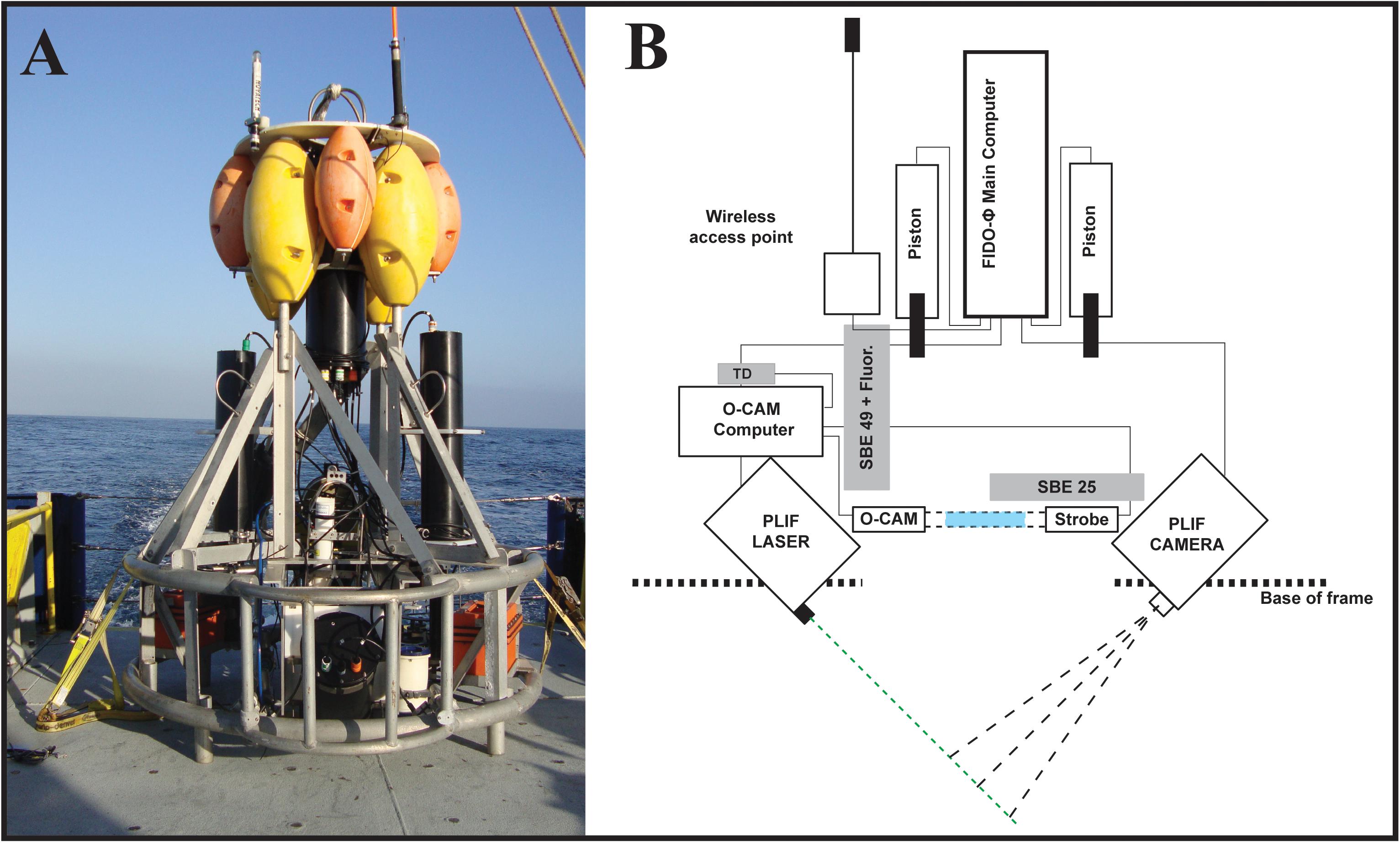
Figure 1. (A) FIDO-Φ/O-Cam on the deck of R/V New Horizon during the August 2011 cruise. (B) Modified schematic from Prairie et al. (2011) to reflect the sensors used for this work. Notice the relative position of the imaging volumes for the PLIF (Intersection of camera and laser dashed lines) and O-Cam (blue rectangle) systems, as well as the location of the imaging volumes with respect to CTD (SBE 25 and SBE 49) and Temperature Depth (TD) sensors.
In spite of taxonomic limitations, in this study we explore the relationships between the fine-scale vertical distributions of chl-a fluorescence, marine snow, and zooplankton. Our analysis puts our observations into the context of functional ecology traits such as feeding preferences. Functional groups, like trait-based ecology, can be used to reduce the complexity of food web analyses imposed by individual species ecological complexities (e.g., Barnett et al., 2007; Pomerleau et al., 2015; Ohman, 2019, and references therein). Here, we provide evidence that the spatial relationships among the nighttime vertical distributions of phytoplankton (measured by chl-a fluorescence), marine snow (quantified as large fluorescent particles), zooplankton grazers, detritivores, carnivores, and omnivores can be explained to a first degree by these generalized functional groups.
The O-cam was mounted on a slow descent, self-ballasted platform named FIDO that was combined with a planar laser imaging fluorometer (PLIF). Together, the system was named the Free-falling Imaging Device for Observing phytoplankton and zooplankton, or FIDO-Φ/O-Cam. The O-Cam was placed immediately above the PLIF imaging volume (Figure 1B). In addition, SBE25 and SB49 CTDs (Sea-Bird Electronics, United States) were placed on the platform; the SBE25 also included an ECO FL fluorometer (Wet Labs). In operation, and by adjusting ballast, the FIDO-Φ/O-Cam system was programmed to maintain a descent rate of approximately 10 cm/s.
The PLIF has been extensively described (Franks and Jaffe, 2001, 2008; Prairie et al., 2010). However, briefly, it consists of a CCD camera (Cooke Sensicam) equipped with a 50 mm Nikor lens (f/1.4 aperture) that images a 6.5 mm thick sheet of light that is parallel to the image plane of the camera (Figure 1B). The light was produced by a 3-W, 532-nm diode-pumped solid-state laser (CVI Melles Griot). The field of view of the camera was approximately 9.8 × 13 cm with a spatial sampling resolution slightly smaller than 100 × 100 μm per pixel that was approximately equal to the true system optical resolution. The camera acquired images at a rate of 1 Hz with an exposure time of 20 ms. Observations were made through a band pass light filter that transmitted light at wavelengths of 670–690 nm, identical to those used by the fluorometer to measure chl-a fluorescence.
The O-Cam imaging system was described in detail in Briseño-Avena et al. (2015), however a brief description is provided here. Designed as a self-contained shadowgraph camera to capture undisturbed images of zooplankton in situ, the system consists of two separate underwater cylindrical housings, one containing a strobing LED light (LedEngine LZ74 2 × 2 Diode Array) and the other a camera (AVT GX1910 × 1080, 5.5-micron pixels, 14 bits). The view ports face each other with the collimated light beam aimed directly into the camera (Settles, 2012). The 71 cm space between the housings’ view ports contains the imaged volume. The O-Cam’s sampling volume, estimated by measuring the distance in which a transparent resolution target is in focus (15 cm) and multiplying by the circular area of the field of view (7.0686 cm2), was 0.106 L per frame. The O-cam was positioned near the bottom of the profiling vehicle and, as such, only O-Cam data from downcasts were analyzed.
PLIF bulk chl-a fluorescence was obtained by integrating the intensity of fluorescence in the images as it is linearly correlated with chl-a fluorescence intensity measured by commercial fluorometers (Franks and Jaffe, 2001; Prairie et al., 2010). Fluorescent particle concentrations were obtained from the fluorescence images following the protocol of Prairie et al. (2010). Images were first corrected for spatial variations in the fluorescence intensity of the incident laser sheet and a fluorescence intensity threshold was then used to define “fluorescent particles” as one or more contiguous pixels with fluorescence intensities greater than the threshold value. The threshold was determined separately for each profile prior to processing. Since the imaging pixel size was ∼100 × 100 μm, and most particles observed had an area of more than one pixel, fluorescent particles here are considered to be primarily marine snow (sensu Alldredge and Silver, 1988). However, we note that they may also include some large individual phytoplankton and chains. Single-pixel fluorescence could be created by particles as small as 20–50 μm in diameter (Zawada, 2002), although their sizes cannot be resolved. A total of 5,906 fluorescence images from nine profiles were analyzed.
O-cam images were manually annotated using a custom-made graphical user interface in Matlab. Every image for all profiles presented here was visually inspected for the presence of zooplankton. In total, 6,116 O-Cam images, spanning nine vertical profiles, were annotated. The annotation consisted of drawing a box around the identified organism and then assigning it to one of 22 predetermined taxonomic categories. These categories were created based on the most common zooplankton observed in early test deployments of the O-Cam. Images were classified at the lowest taxonomic level possible. For this work, the most abundant categories were: hydromedusae, euphausiids, calanoid copepods, cyclopoid copepods, and appendicularians (Figure 2). Concentration estimates (individuals per liter) were obtained by dividing the number of observations in each frame by the volume sampled per frame (0.106 L). To test the quantitative capabilities of the O-Cam, the image-derived zooplankton concentration (Individuals L–1) estimates were previously compared to those obtained from net samples collected with a 1 m2, 202 μm mesh size MOCNESS (Supplementary Material).
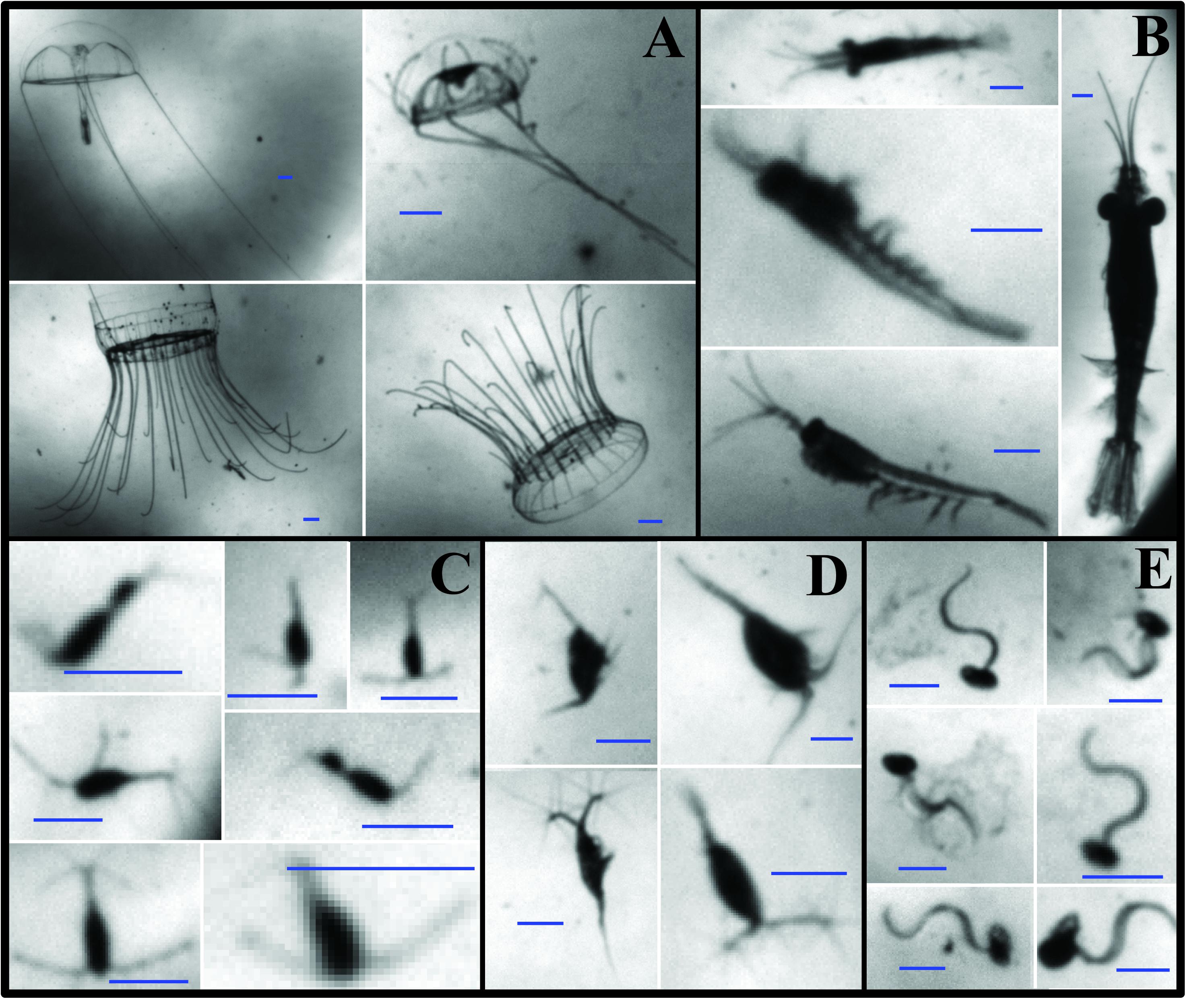
Figure 2. Examples of zooplankton images from the O-Cam system. (A) Hydromedusae; (B) Euphausiids; (C) Cyclopoid copepods; (D) Calanoid copepods; (E) Appendicularians. All the scale bars are 1 mm long.
The FIDO-Φ/O-Cam cruise was conducted near the head of a submarine canyon at the northern end of the Santa Catalina Basin aboard the R/V New Horizon during August 18–23, 2011 (triangle symbol in Figure 3). This region was chosen because SCM layers and zooplankton grazers have been extensively studied here (Cullen, 1982; Napp et al., 1988) thereby enhancing our chances of capturing these features. Hence, fine-scale nighttime vertical distributions of zooplankton and phytoplankton were resolved using the FIDO-Φ/O-Cam. These data were used to reconstruct the in situ concurrent distributions of chl-a fluorescence, fluorescent particles (consisting primarily of marine snow), and zooplankton, along with hydrographic properties.
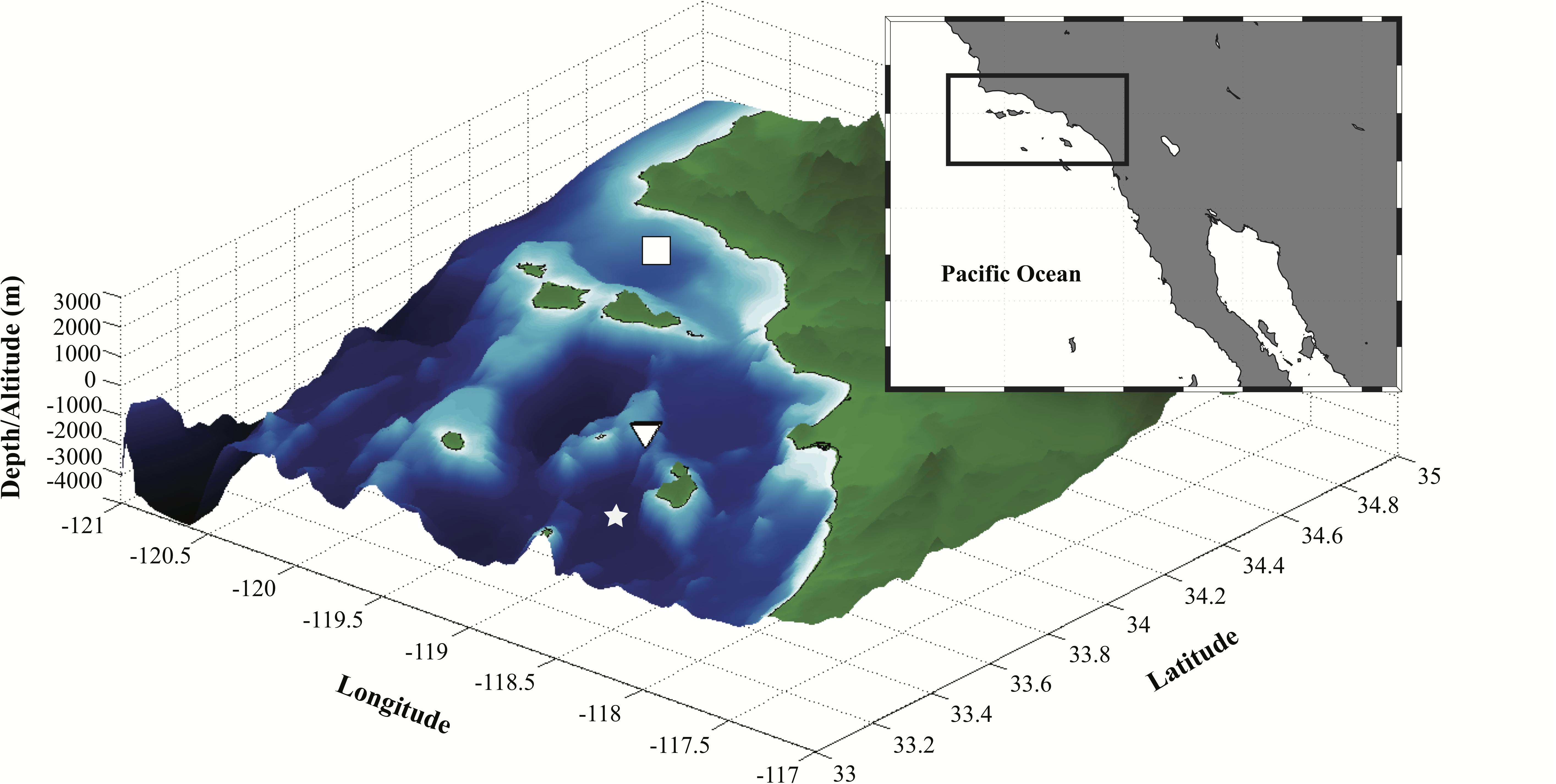
Figure 3. Bathymetry of the study region (area bounded by the solid black rectangle in the inset map). White square indicates the general location of the Santa Barbara Channel sampling sites for the CalEchoes cruise aboard R/V Melville from September 26–October 1, 2010 (see Supplementary Materials). Inverted triangle represents the site occupied during the FIDO-Φ/O-Cam cruise aboard R/V New Horizon from August 18–23, 2011. White star indicates the location of the Santa Catalina Basin.
Over successive nights, the FIDO-Φ/O-Cam platform was deployed in the same general location. Deployments were limited to nighttime to avoid contamination of the PLIF images by ambient sunlight (Franks and Jaffe, 2008). Furthermore, higher zooplankton biomass in this region tend to coincide with the SCM at night, when diel vertical migrators have reached their nighttime locations (Napp et al., 1988). Nighttime profiling also enhanced the chances of imaging a depth-dependent diverse group of zooplankters, given the relatively small imaged volume of the O-Cam system. Each FIDO-Φ/O-Cam deployment was composed of three consecutive vertical profiles; data were acquired during the downcasts to a maximum depth of 75 m. After each drop cycle was completed, the platform was recovered for data download and system updates, such as battery recharging or replacement. Because the platform drifted with the water currents, the ship was repositioned to the original drop location centered at 33° 33′N and 118° 54′W before the FIDO-Φ/O-Cam was re-deployed for a new cycle. While this repositioning can be counter-intuitive for a self-contained, free-descent platform, we were not seeking to conduct a Lagrangian experiment, but rather we wanted to observe potential changes in zooplankton assemblage distributions as internal waves passed through the same sampling region. Nine profiles from four cycles collected over two consecutive nights (each one labeled by its “Drop_Profile” identifying number) when all the sensors were fully functional were chosen for the present analysis (Table 1).
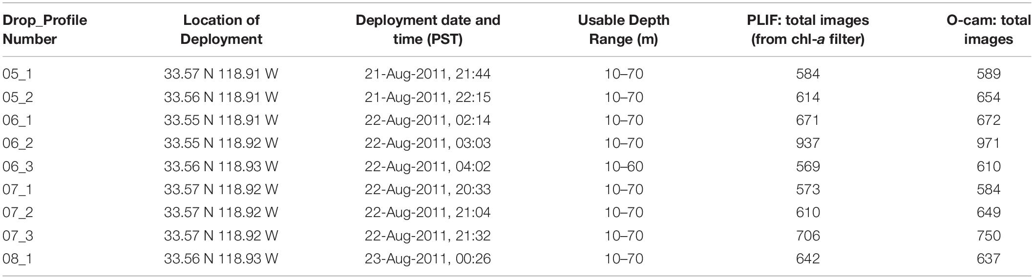
Table 1. FIDO-Φ/O-Cam cruise “Drop_Profile” information.
As most instruments had their own pressure sensors, all data from a given profile were merged based on depth. The PLIF imaging volume was 0.8 m below the depth sensor and this offset was incorporated into the analysis before merging with the other data. Because the O-Cam was self-contained and had its own temperature-pressure (TP) sensor, no depth corrections were necessary. After data merging, each variable was independently binned by depth using a 0.3 m bin size and then smoothed over 1.5 m using LOWESS to remove small-spatial-scale noise. The result was a fixed-size data vector for each variable, giving profiles that could be compared to each other using regular depth coordinates. In addition, data from the PLIF, SBE 25-ECO FL, SBE 49 and O-Cam were binned in density coordinates using a density bin size of 0.09 kg/m3. This bin size was found empirically to be the minimum size that would allow adequate observations per bin, given the density range of 1023.8 to 1026.1 kg/m3.
All biological profile concentrations were normalized in depth and density coordinates by dividing all the values in a given profile by its maximum. The normalized values thus ranged between zero and one. Normalization allowed comparisons across all profiles, particularly when profiles were dominated by a data point of particularly high intensity. Then, canonical profiles were estimated by averaging the individual normalized profiles in density coordinates over time. This time averaging was justifiable given the spatial and temporal proximity of drops and profiles (Table 1), and the consistent distributions of properties among different normalized profiles. In the case of CTD fluorescence intensity and PLIF fluorescent particles, this data processing step resulted in the normalized Fluorescence Intensity (FIn) and Fluorescent Particles (FPn; primarily composed of marine snow) variables. Both, non-normalized and normalized data are reported here.
A cross-correlation analysis was done to determine the vertical offset (i.e., decoupling, in density coordinates) between the FIn and FPn canonical profiles. Cross-correlation analyses were similarly conducted to determine the vertical offset between zooplankton canonical profiles and the FIn and FPn canonical profiles. The spatial lags for all cross-correlation analysis outputs were reported as vertical density offsets in density units (kg/m3) while retaining the sign (±) of the signal lag. Finally, we also calculated the absolute differences between FIn and FPn offsets (i.e., |FIn offset - FPn offset|) for each taxon to examine the decoupling magnitude from each taxon and both fluorescence parameters combined.
Vertical gradients of the FIn and FPn canonical profiles in density coordinates were calculated using the following equations:
where Δρ = 0.09 kg/m3 in both cases, and FIn and FPn denote normalized, time-averaged fluorescence intensity and PLIF fluorescent particle concentration, respectively (referred to as canonical profiles for these variables).
Zooplankton peaks were identified in the raw, time-averaged counts for each zooplankton group (Supplementary Figure 2). Briefly, we defined a peak of the vertical distribution of each zooplankton group to be those values having a greater than 95% probability of being higher than the background (mean) count in any given density bin (0.09 kg/m3 per bin).
The slow descent of the FIDO platform and the high sampling rate of the sensors yielded fine-scale (cm) distributions of physical and biological data, uncontaminated by ship heave motions. During our field work, salinity did not vary substantially (Figure 4A); the water column was thermally stratified, with the thermocline occurring between 25 and 30 m depth (Figure 4B). A fluorescence intensity maximum was located within the thermocline in all profiles (Figure 4C). Fluorescent particles (marine snow) were found below the thermocline, and one profile (6_3) had more than twice the concentration of particles than any other profile during the deployment cycles (Figure 4D). Total zooplankton concentrations were located in the warm surface waters, above the thermocline and the fluorescence intensity maximum; furthermore, total zooplankton was patchily distributed both with depth and over time (Figure 4E). Hydromedusae, appendicularians, and calanoid copepods were found in warmer waters (Figures 4F–H). Cyclopoid copepods showed higher concentrations in colder waters, below the thermocline and fluorescence intensity maximum (Figure 4I). Euphausiids were widely distributed throughout the water column but were located in warmer waters in the first half of the profiles and deeper in colder waters in the second half (Figure 4J).
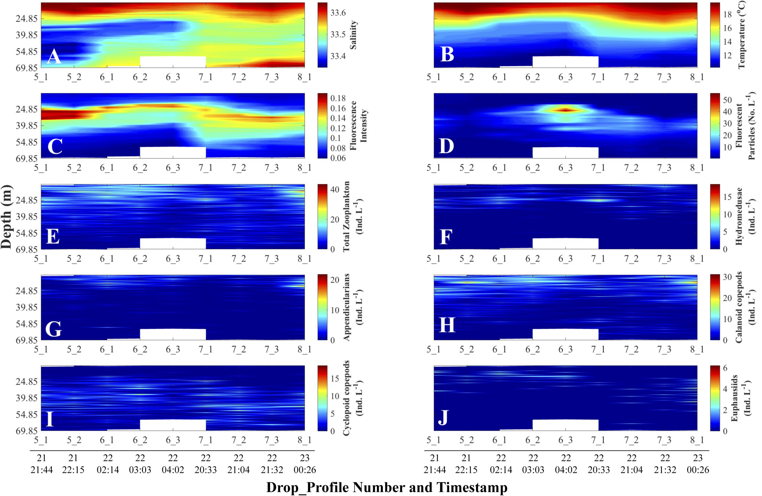
Figure 4. Depth-time distributions of physical and non-normalized biological data. Day and time (all in August 2011, Pacific Standard Time) are at the bottom of each column and apply to all the panels above the line of timestamps. Full details on each Drop_Profile can be found in Table 1. (A) Salinity; (B) Temperature (°C); (C) Fluorescence Intensity (SBE 25 fluorometer); (D) Planar Laser Imaging Fluorometer (PLIF) fluorescent particle concentration (Numbers L–1); Panels (E) through (J) represent O-Cam zooplankton concentrations (Individuals L–1): (E) Total zooplankton; (F) Hydromedusae; (G) Appendicularians; (H) Calanoid copepods; (I) Cyclopoid copepods; and (J) Euphausiids.
The vertical displacements of the fluorescence intensity maximum evident in the fluorescence versus depth profiles (Figure 4C) followed the displacements of isotherms (Figure 4B) – temperature being the main determinant of density during our study, as evidenced by the larger variations in temperature than salinity in surface waters (Figures 4A,B). While there could be other potential contributors, we attributed such vertical displacements to passing internal waves and/or the internal tide. Tide charts (data not shown) for the nearest location to our sampling site (Catalina Harbor, Santa Catalina Island; 33° 25.8′ N, 118° 30′ W) showed that the vertical displacement of the isotherms (Figure 4B) were synchronous with the local tide during the cruise sampling dates (Table 1). The density-binned data (Figure 5) showed that the vertical displacements visible among depth profiles disappeared when using density coordinates, confirming that fluorescence intensity followed isopycnals rather than pressure surfaces (i.e., depth layers). Not obvious in Figures 4, 5 are vertical displacements of the fluorescent particle concentration profiles due to the substantially higher signal in profile 6_3 than the profiles before and after. This inter-profile variability in total concentration was removed by normalizing each variable by its maximum value in a given profile (see “Materials and Methods section”). These normalized vertical distributions of each variable now range between zero and one in each profile (Figure 6).
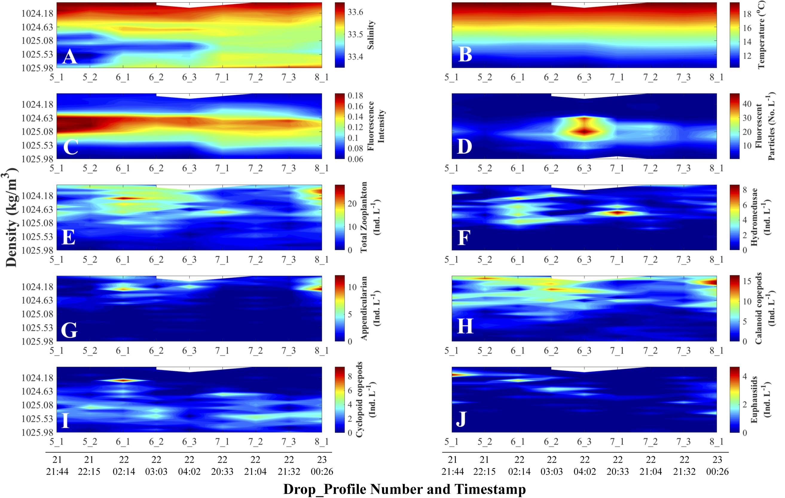
Figure 5. Density-time distributions of physical and non-normalized biological data. Day and time (all in August 2011, Pacific Standard Time) are at the bottom of each column and apply to all the panels above the line of timestamps. Full details on each Drop_Profile can be found in Table 1. (A) Salinity; (B) Temperature (°C); (C) Fluorescence Intensity (SBE 25 fluorometer); (D) Planar Laser Imaging Fluorometer (PLIF) fluorescent particle concentration (Numbers L–1); Panels (E) through (J) represent O-Cam zooplankton concentrations (Individuals L–1) data: (E) Total zooplankton concentration; (F) Hydromedusae; (G) Appendicularians; (H) Calanoid copepods; (I) Cyclopoid copepods; and (J) Euphausiids.
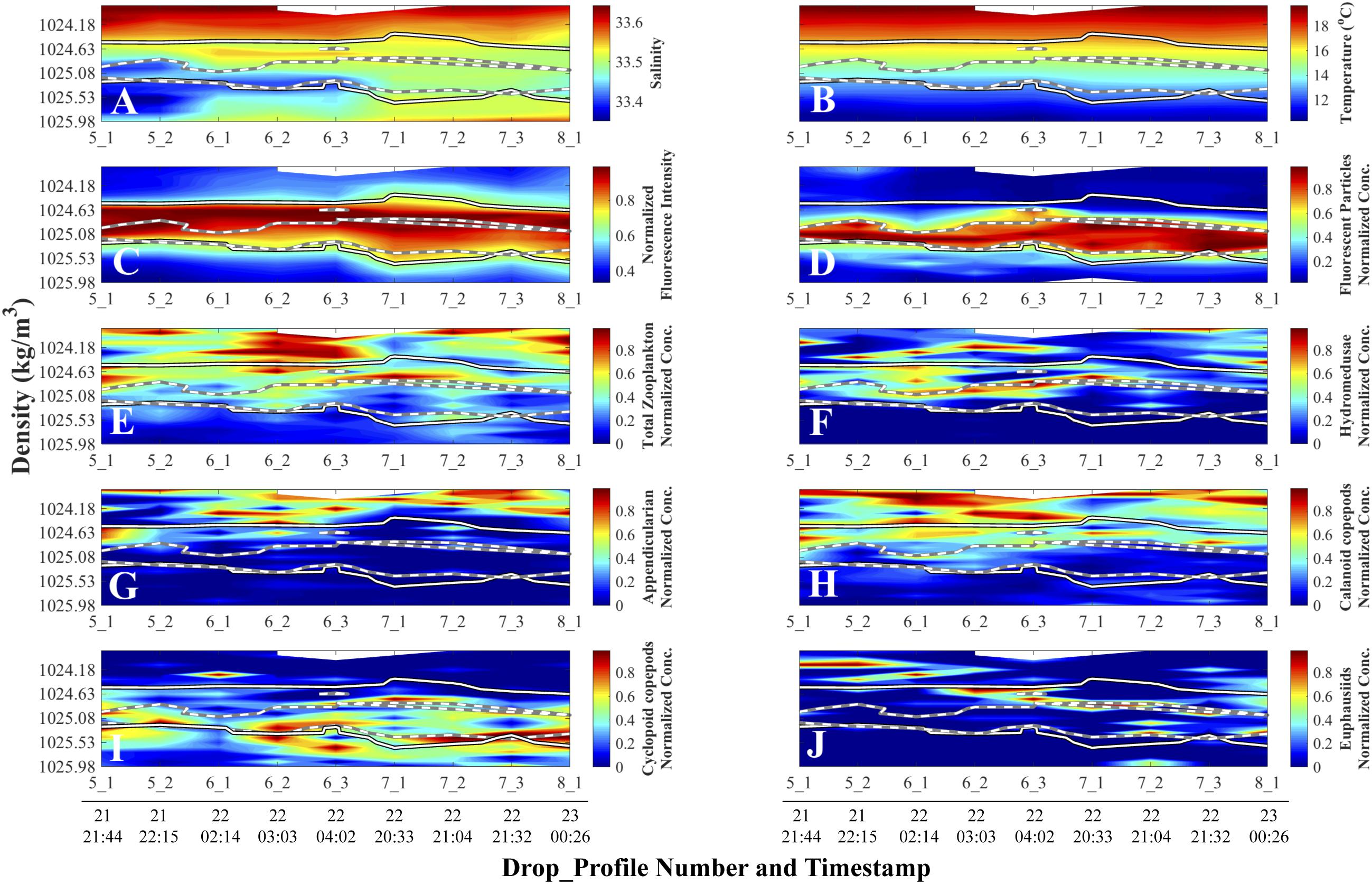
Figure 6. Density-time distributions of physical and normalized biological data. Day and time (all in August 2011, Pacific Standard Time) are at the bottom of each column and apply to all the panels above the line of timestamps. Full details on each Drop_Profile can be found in Table 1. (A) Salinity; (B) Temperature (°C); (C) Fluorescence Intensity (SBE 25 fluorometer); (D) Planar Laser Imaging Fluorometer (PLIF) fluorescent particle normalized concentration. Panels (E) through (F) represent O-Cam zooplankton normalized concentrations: (E) Total zooplankton; (F) Hydromedusae; (G) Appendicularians; (H) Calanoid copepods; (I) Cyclopoid copepods; and (J) Euphausiids. Solid lines superimposed on panels represent the 70% threshold normalized Fluorescence Intensity from panel (C), and white-on-black lines superimposed on panels represent the 70% threshold fluorescent particle normalized concentration contour from panel (D).
Once data plotted in density coordinates were normalized, patterns that were obscured in the depth and density/non-normalized plots became strikingly evident (Figure 6). In this concentration-normalized, density-coordinate frame of reference, two maxima were identified: a subsurface chlorophyll maximum (SCM; Figure 6C) and a fluorescent particle concentration maximum, from here on referred to as the fluorescent particle maximum (FPM; Figure 6D), which was composed primarily of marine snow. While the FPM overlaps with the SCM, the peak intensities of the features were offset from one another, with the FPM peak being located in denser (deeper) waters than the SCM (Figures 6C,D).
The normalized total zooplankton concentrations distributions were found mostly above both the SCM and FPM (Figure 6E). However, different taxa showed distinct distributions with respect to the maxima, and no individual zooplankton taxon was found exclusively within either the SCM or the FPM. Hydromedusae showed some overlap with the SCM but were mostly located above the FPM (Figure 6F). Similarly, appendicularians and calanoid copepods (Figures 6G,H) were mainly located above both the SCM and FPM. Cyclopoid copepods were mainly concentrated at the lower boundary of the FPM (Figure 6I). Euphausiids showed a more even vertical distribution, with some located above the FPM at the beginning of the cruise and within it toward the end (Figure 6J).
The time-averaged profiles (canonical profiles) for each variable revealed different relationships among FIn and FPn, and the zooplankton canonical distributions in relation to each of the two fluorescent variables (Figure 7) as quantified by the cross-correlation analyses are described below.
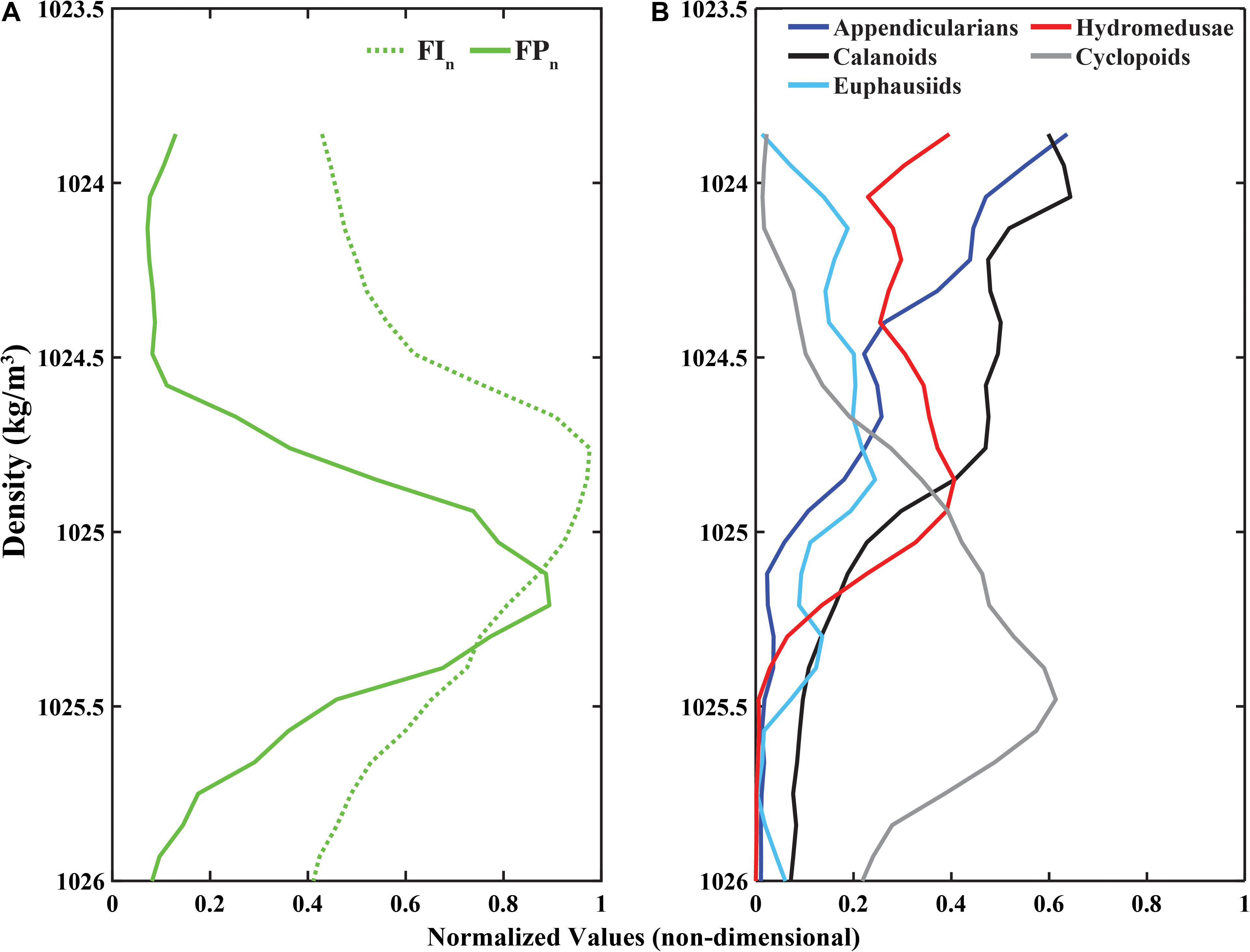
Figure 7. Canonical profiles (time-averaged normalized values in density coordinates) for (A) Fluorescence Intensity (FIn; green dotted line) and Fluorescent Particles (FPn; green solid line), and (B) appendicularians, calanoid copepods, cyclopoid copepods, euphausiids, and hydromedusae.
The cross-correlation of FIn and FPn showed a peak correlation at a vertical displacement in density coordinates of −0.18 kg/m3 (i.e., the FPn main signal peak was deeper than the FIn main signal peak by two density bins, recalling that each density bin was 0.09 kg/m3 wide) as shown in Figure 7A. These peaks in the FIn and FPn represent the core of the SCM and FPM shown in Figures 6C,D. The peak cross-correlations between zooplankton canonical profiles and FIn, and FPn all occurred at non-zero vertical offsets (Table 2), confirming that the main signal peak in each zooplankton group fell above or below the main signal peaks in both FIn, and FPn, although to varying degrees, indicating different degrees of decoupling between taxa and the SCM and FPM. With the exception of cyclopoid copepods, all zooplankton groups showed consistently larger vertical density offsets with respect to FIn than to FPn, although the magnitude of this offset varied among zooplankton groups (Table 2). The differences in vertical offsets were directly affected by the shape of the canonical profile of each taxa (Figure 7B). Cyclopoid copepods were the only group whose canonical profile peaked deeper than both the SCM and the FPM, as indicated by negative vertical density offsets relative to FIn (−0.36 kg/m3) and FPn (−0.18 kg/m3). Yet their offset difference (0.18 kg/m3) indicate some degree of coupling with the SCM and FPM (Figure 7, gray line). Calanoid copepods and appendicularians, with consistent higher relative abundances in the upper water column, had the largest vertical density offsets of all zooplankton groups with respect to FIn (0.63, 0.72 kg/m3, respectively) and FPn (0.90, 0.99 kg/m3, respectively) but, interestingly the same offset difference value of 0.27 kg/m3, showing a similar degree of decoupling with respect to the SCM and FPM (Figures 7A,B, black and dark blue lines). Hydromedusae had vertical density offsets of 0.36 and 0.45 kg/m3 with respect to FIn and FPn, respectively, and smaller differences between offsets (0.09 kg/m3) than all other groups (Table 2), indicating a close coupling with the SCM and FPM (Figure 7, red line). Euphausiids had a smaller vertical density offset with respect to FIn (0.18 kg/m3) than with FPn (0.54 kg/m3) and was the group with the largest vertical density offset difference (0.36 kg/m3) of all the zooplankton groups, and therefore the group that showed the highest degree of decoupling from both SCM and FPM (Figure 7, light blue line). However, the canonical profile of the euphausiids may reflect that their vertical distributions changed over the duration of the study, unlike the other zooplankton groups.
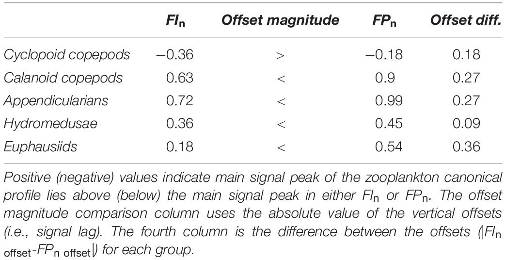
Table 2. Cross-correlation lag/vertical offset values in density (kg/m3) coordinates between FIn, FPn, and each canonical profile for zooplankton groups.
The shape of the SCM and the FPM differed with regard to the sharpness of their upper and lower gradients. The SCM was characteristically asymmetric, with one distinct, sharp gradient forming its upper boundary, and a gradient about half the magnitude of the upper, forming its lower boundary (Figure 8A). The FPM, on the other hand, was symmetric, bounded by two vertical gradients of similar magnitudes (Figure 8B). Peaks in the zooplankton vertical distributions showed different associations with the SCM, the FPM, and their vertical gradients (Figure 8). Hydromedusae (carnivorous) peaks were distinctly associated with the SCM, with only one peak (of minor relative intensity) within the upper SCM gradient. No hydromedusae peaks were found within the deeper SCM gradient (Figure 8A; red stars). At the same time, hydromedusae peaks were associated with the FPM upper gradient (Figure 8B; red stars), but not with the FPM itself. Euphausiids (carnivores/omnivores) had two peaks, the largest of which was associated only with the upper SCM gradient, but not the SCM itself (Figure 8; light blue diamonds). Calanoid copepods (considered herbivores here although the group potentially includes omnivores) were found mostly above the upper SCM gradient and SCM, with only one calanoid peak (of medium relative intensity) located within the SCM (and by extension within the decaying slope of the upper gradient; Figure 8A; black squares). Calanoid copepods had no association with the FPM, with one notable exception: one of the medium-intensity peaks occurred in the steeper slope of the upper FPM gradient (Figure 8B; black squares). Cyclopoid copepods (herbivores and detritivores) were not fully associated with the SCM or the FPM. However, the cyclopoid copepods’ most intense peak was co-located within the deeper gradients of these features, with two minor cyclopoid peaks above (but within the FPM; Figure 8B; gray triangles) and five peaks of medium, but decreasing in intensity, below the deeper SCM/FPM gradients. Finally, appendicularians (filter-feeders) were not clearly associated with either the SCM, the FPM, or their gradients. However, their higher concentrations were consistently located above the SCM and FPM (Figure 8; dark blue circles), and were closely associated with the strongest calanoid copepod concentration peaks.
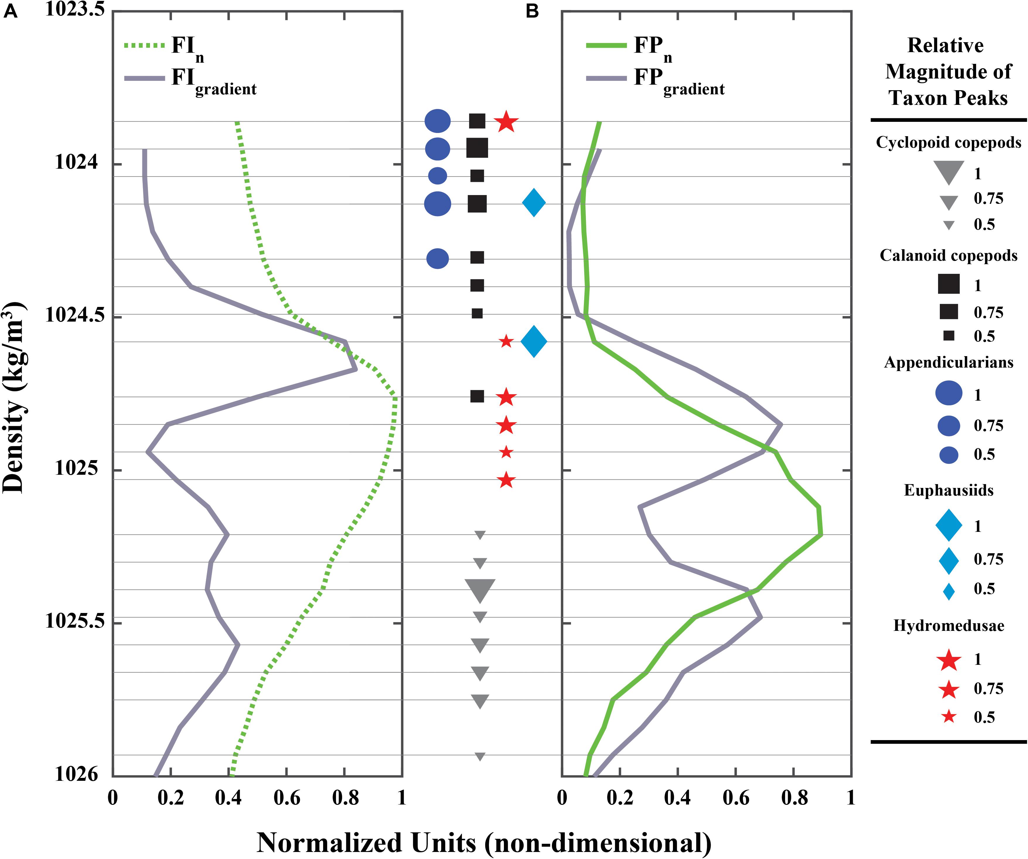
Figure 8. (A) Normalized, time-averaged Fluorescence Intensity (FIn) profile (green dotted line) and its vertical gradient (FIgradient; gray solid line). (B) Normalized, time-averaged PLIF Fluoresence Particles (FPn) profile (green solid line) and its vertical gradient (FPgradient; gray solid line) in water density space. Markers (sizes are relative magnitude of raw counts of the peak) between (A,B) represent zooplankton peaks (95% probability of being higher than background values; see Supplementary Figure 2) and are the thin gray horizontal lines show their vertical position in relation to (A,B). Colors are the same as in Figure 7B for each zooplankton group: calanoid copepods (black squares), cyclopoid copepods (gray triangles), appendicularians (dark blue circles), euphausiids (light blue diamonds), and hydromedusae (red stars).
Subsurface chlorophyll maxima (SCM) are ubiquitous features of marine and freshwater ecosystems (Cullen, 2015), and considerable research has explored the roles of bottom-up controls, including light, thermal stratification, and nutrients in shaping the SCM (e.g., Cullen, 2015; Leach et al., 2018). Thus, the persistent peak in FIn observed throughout this study (representative of a SCM) is not surprising, particularly in our stratified coastal region study site. More recently, studies have found that marine snow can also form layers, which are often ubiquitous features of stratified systems (MacIntyre et al., 1995; Alldredge et al., 2002, Prairie and White, 2017). The fluorescent particle maximum (FPM) we observed similarly represents a peak in marine snow concentration, although the vertical scale, while narrower than the SCM, was substantially wider than the vertical scale of thin layers as they are typically classified (Dekshenieks et al., 2001).
In our data, the FPM was distinct from the SCM (with the FPM sitting deeper in denser waters, albeit with apparent overlap. Figure 7A), which is consistent with Prairie et al. (2010) who observed (also with the FIDO-Φ) cryptic peaks containing large fluorescent particles (primarily marine snow) that sat below the sub-surface chlorophyll maximum. This pattern confirms that the profiles of bulk chl-a fluorescence and fluorescent particles detected by the PLIF have different compositions; while the bulk chl-a fluorescence is dominated by individual phytoplankton representing a wide range of sizes, the fluorescent particles are large and likely composed primarily of marine snow. The relationship between the SCM and the FPM observed here (Figure 7A) is reminiscent of a marine snow layer observed forming 1–2 m below a diatom bloom (Alldredge et al., 2002). Similarly, isolated layers or diatom flocs formed by Pseudo-nitzschia off Monterey Bay, California were detected by an imaging system, but not by standard fluorometers (Timmerman et al., 2014). Although our data cannot distinguish between detritus of phytoplanktonic origin and that derived from other organic material (e.g., discarded appendicularian houses, decomposing plankton, fecal pellets), the difference in the depths of the SCM and the FPM is notable, considering that they may represent different food sources for different zooplankton grazers. This observation is not trivial, especially given laboratory observations of food selectivity (live phytoplankton vs. detritus) by the copepod genera most likely present in our imagery: Pseudocalanus, Acartia, and Temora (DeMott, 1988).
In most cases, the SCM is thought to be a region of intense biological activity, including remineralization, primary production, grazing, predation, sexual reproduction, and infection (Cullen, 2015 and references therein). Similarly, marine snow accumulations have been suggested as potential hotspots for feeding by zooplankton (e.g., Alldredge et al., 2002; Möller et al., 2012). However, the impacts of higher trophic-level processes on the SCM have rarely been studied. Only recently global biogeochemical models have revealed the potential of top-down microzooplankton control of the SCM, for example (Moeller et al., 2019). Quantifying the effects of larger heterotrophic grazers, however, has been difficult. This knowledge gap is partially because sampling these organisms at the spatio-temporal scales of the SCM is difficult in the field – a problem obviated by the recent introduction of in situ imaging technologies. Still, relatively little is known about how in situ distributions of various zooplankton taxa relate to those of marine snow and the SCM simultaneously.
Despite the known strong trophic links between zooplankton grazers and both phytoplankton and marine snow, we were surprised to find a spatial mismatch between the vertical distributions of all zooplankton taxa and these two potential food sources. As revealed by the cross-correlation analyses, the main peaks of all groups of zooplankton were vertically offset from the main peaks of both fluorescence intensity (representing phytoplankton) and fluorescent particles (representing marine snow). The direction and extent of this vertical offset, however, depended on taxon, with cyclopoid copepods being found below both the SCM and FPM, and the other zooplankton (calanoid copepods, appendicularians, and euphausiids) found either slightly or substantially above both the SCM and FPM. Offsets between copepods and the SCM were observed by Harris (1988) in the stratified summer waters of the English Channel. Harris, however, found the calanoid copepods Paracalanus parvus and Centropages typicus peaked above the SCM, whereas the cyclopoids Oncaea subtilis and Oithona similis were located immediately above and within the SCM, respectively. Other calanoid copepods in the same study showed a bi-modal distribution, where some peaks were co-located with the SCM or below in deeper waters. Interestingly, the SCM in that work and this one occurred at about the same depth (20–25 m). However, we observed quite different distributions of copepods relative to the SCM.
Not much could be inferred from our current data on appendicularians, which were observed mainly in the upper water column, and not associated with either the SCM or the FPM. In a location close to our sampling area, Alldredge (1982) found that a shallow aggregation of Oikopleura longicaudata was due to a spawning event – she observed sexually mature individuals (free swimming; that is, without “houses”), as well as juveniles and eggs. Our observations included numerous free-swimming (no houses attached), potentially sexually mature appendicularians mainly from the genus Oikopleura. Appendicularians are filter feeders, capable of preying on bacterioplankton and phytoplankton, including ciliates (Lombard et al., 2010). An alternative hypothesis to their presence in the region above both SCM and FPM would be that they were feeding on high concentrations of bacteria or organisms not sampled by our devices, neither of which can be tested using our data.
Our observations of hydromedusae distributions suggest that these predators may have affected how herbivorous grazers interacted with their food sources. Gaps in our understanding of this predator-prey relationship stem from gelatinous organisms, including hydromedusae, being severely damaged by nets (Ohman, 2019), making it difficult to identify and quantify them, let alone observe their fine-scale distributions with respect to physical and biological factors in situ. One of the most striking examples that emerged from this analysis was the distribution of hydromedusae, which are considered primarily carnivorous, within the SCM (Figure 8A; red stars) and above the FPM (Figure 8B; red stars). Another distinct peak of high relative hydromedusae concentration is also located in the lowest density values at the top of the water column, and not associated with either the SCM or FPM (Figure 8). Interestingly, Napp et al. (1988) did not find any relationship between medusae (although no details were provided on what types of medusae were quantified in their work) and the SCM in a study conducted in the same region where our field work took place.
Hydromedusae are known to feed on copepods and appendicularians (e.g., Fulton and Wear, 1985; Costello and Colin, 2002). In our data, the hydromedusae group was composed of at least 6 different body types, and most likely different species, all present in every FIDO-Φ/O-Cam profile: the narcomedusae Solmaris sp. and Solmundella bitentaculata; the trachymedusae Liriope tetraphylla, Crossota sp., and at least two other unknown species. Some of these species (L. tetraphylla) are known to cause regime shifts in crustacean zooplankton assemblages (Yilmaz, 2015) and some species (including narcomedusae) have been observed feeding on appendicularians and crustaceans (among other prey), especially at night (Madin, 1988). In micro-scale (cm) laboratory experiments, Frost et al. (2010) found that hydromedusae tended to aggregate at density discontinuities where phytoplankton and calanoid copepod layers were located at the beginning of the experiment. In addition, they also noted that while hydromedusae (Nemopsis bachei) remained in these layers, the calanoid copepods (Acartia tonsa) dispersed during the same period, avoiding their predators. In our work, high-concentration peaks of calanoid copepods and appendicularians occurred above the SCM (black squares and blue circles in Figure 8A). These distributions are interesting because the largest peaks of hydromedusae seemed to bracket all major peaks observed for calanoid copepods and appendicularians. We believe that this pattern may indicate predator avoidance by the latter groups, a particularly interesting pattern given the fact that these relationships persisted over the two consecutive nights of our fieldwork.
An additional, but not necessarily mutually exclusive, hypothesis is that hydromedusae were feeding on phytoplankton and marine snow during this field work, as their largest peaks were associated with both the SCM and FPM (Figure 8). Although there is plenty of evidence that hydromedusae benthic stages can consume bacteria, protozoa, phytoplankton, detritus, and even dissolved organic matter (Gili and Hughes, 1995, cited in Bouillon et al., 2004), fewer reports exist for the free-swimming hydromedusa stages. Working on a species not found in our imagery (Blackfordia virginica), Morais et al. (2015) were surprised to find diatoms and dinoflagellates in the guts of these field collected hydromedusae. Colin et al. (2005) found that the trachymedusa Aglaura hemistoma effectively fed on chlorophyll-bearing protists, in addition to copepods and nauplii, effectively labeling this hydromedusa as an omnivore. It is possible that the trachymedusae and narcomedusae found in this study, generally recognized as primarily carnivorous, were feeding on primary producers, and potentially on marine snow. While our data cannot answer this question, the position of these hydromedusae within both the SCM and FPM, in addition to the limited but conclusive evidence in the above-mentioned studies, support this hypothesis.
Several studies have suggested that peaks in food abundance may not be the most important determinant of grazer distribution, but rather the gradients in food abundance (Leising et al., 2005; Prairie et al., 2011). The presence of high-density aggregations of zooplankton immediately above or below thin layers of phytoplankton and marine snow has been observed in stratified systems, in both shallow and deep waters (e.g., Benoit-Bird et al., 2009; Möller et al., 2012; Greer et al., 2013, 2020). In many cases, previous studies concluded that the sharp vertical gradients in the concentrations of phytoplankton and marine snow were caused by their consumers (Alldredge et al., 2002; Benoit-Bird et al., 2009; Möller et al., 2012). Here we examine how the distributions of herbivorous zooplankton taxa and their potential responses to predators might explain the shape of the distributions of their food sources.
The upper boundary (and sharpest gradient) of the SCM coincides with a peak in euphausiids and overlaps with peaks in calanoid copepods. The interplay of the predatory hydromedusae located at the SCM, potentially driving their (herbivorous grazer) prey upward may help explain the shape of this upper boundary. While it is recognized that copepods have been found above the SCM grazing on higher-quality food sources within the region of maximum primary productivity – a common mechanism invoked to explain the formation and maintenance of SCM layers (Cullen, 2015 and references therein) – it may also be possible that predator avoidance may drive herbivorous grazers upward, enhancing the grazing on the phytoplankton above the SCM, which in turn could shape the phytoplankton gradients forming the SCM. It is harder to interpret the location of euphausiids in relation to the SCM given their widely known diel vertical migration behavior (e.g., De Robertis, 2002; Werner and Buchholz, 2013) and the fact that their vertical distribution changed over the duration of our study.
The dynamics shaping the lower SCM boundary are more difficult to discern, because the bulk fluorescence signal includes some marine snow. This overlap in signal sources is perhaps evident in the secondary, less-sharp gradient (that is, below the SCM) in the bulk fluorescence signal (gray line in Figure 8A), which aligns with the FPM. Alldredge et al. (2002) observed the in situ formation of a marine snow layer, deriving from growth and subsequent sinking of phytoplankton two meters above that layer. Because the FPM in this work was primarily composed of fluorescence particles, it is reasonable to hypothesize that the FPM could be maintained by aggregation and sinking of phytoplankton from the SCM above.
Marine snow layers form by sinking particles, which can slow down when passing through sharp density gradients, providing an explanation for why marine snow layers are often found associated with density transitions (Prairie et al., 2015; Prairie and White, 2017). This mechanism may also apply to the FPM observed in the present work, despite the fact that the peak we observed is wider (∼5–10 m; Figure 4D) than many of the marine snow layers previously observed by others (10 s of cm; e.g., Alldredge et al., 2002). The shape of the FPM we observed was roughly symmetrical, with two sharp gradients of similar magnitude above and below the maximum (Figure 8B; gray line). Layers formed solely by decreases in settling velocity are predicted to have sharper gradients at the upper boundary (Prairie and White, 2017), which may indicate that different mechanisms generated the upper and lower boundaries of the FPM observed here. A decrease in sinking velocity may explain the sharp gradient above the maximum, and the sharp gradient below it may be explained by a combination of losses to sinking and consumption by cyclopoid copepods, which were found immediately below the FPM in its lower boundary (Figure 8B; gray triangles). The same predator-prey argument invoked above for calanoid copepods and appendicularians could be made in the case of the FPM and cyclopoid copepods – that is, cyclopoids were located where their potential predators were not. However, another possibility stems from the complex feeding ecology of cyclopoid copepods, which, in addition to being ambush predators (Paffenhöfer, 1993; Saiz et al., 2014; Kiørboe et al., 2015), are also known to feed on marine snow and fecal pellets of calanoid copepods (Turner, 1986; González and Smetacek, 1994). The fact that cyclopoid copepods have been observed to repackage larger particles into smaller, potentially slowly sinking marine snow (González and Smetacek, 1994) these copepods may have contributed to the symmetrical shape of the FPM feature studied here. These observations are also consistent with the “coprophagous filter” hypothesis; metazooplankton activities in the epipelagic reduce the vertical fluxes of large marine snow (González and Smetacek, 1994; Turner, 2015 and references therein). Unfortunately, we cannot conclusively say that cyclopoids were feeding on marine snow, as no grazing measurements or gut content analyses were conducted. Neither can we rule out other biological processes taking place, including grazing on marine snow by other organisms.
Our fine-scale observations of the vertical distributions of chl-a, marine snow, and zooplankton with different feeding preferences allowed us to infer the trophic drivers underlying the observed spatial distribution patterns of the SCM and FPM. These inferences were possible through the combined deployments of new in situ technologies developed for this purpose. Even though the “enduring enigma” of SCM dynamics has been deemed a mystery solved (Cullen, 2015), the observations presented in our work open new avenues of scientific inquiry, allowing us to develop new hypotheses that could be tested using models of the dynamics of top-down controls on subsurface chlorophyll maxima and marine snow distributions in a variety of aquatic environments, and to evaluate how climate change might alter these dynamics. With the sophistication of in situ sensors, sampling methods, and mathematical models, these approaches could inform each other (Everett et al., 2017), so in future studies, measurements of diel biological rates (primary production, grazing, predation), and measurements of bacterial growth and distribution patterns, along with fine-scale in situ imaging will be important in further elucidating the trophic interactions that we hypothesized, based on our data. Evaluating these hypotheses might be possible with the development and potential availability of new in situ molecular systems (e.g., Spanbauer et al., 2019) especially when they are deployed on multi-sensor platforms.
The datasets generated for this study are available on request to the corresponding author.
JJ, PF, and CB-A contributed to the conception, design, and execution of the study. JP processed PLIF imagery. CB-A processed O-Cam, MOCNESS and Zooscan data, and performed the data analyses. CB-A wrote the first draft of the manuscript. All authors contributed to manuscript revision, read and approved the submitted version.
The bulk of this work is the result of CB-A Ph.D. dissertation work, which was supported by the Mexican agency CONACyT and its UC system partner UC MEXUS.
The authors declare that the research was conducted in the absence of any commercial or financial relationships that could be construed as a potential conflict of interest.
CB-A would like to thank UC Ship Funds for funding the CalEchoes cruise and the CCE-LTER program for the generous support to conduct MOCNESS tows and for providing materials and equipment necessary to process the zooplankton samples. Thanks to Jesse Powell who helped sort zooplankton net samples with the Zooscan. We are thankful to the members, past and present, of the Jaffe Lab who worked hard in setting up the FIDO-Φ platform, especially Paul Roberts, Fernando Simonet, and Fred Uhlman. We thank Michael Ford (NOAA) for providing taxonomic identification of selected hydromedusae images. The fieldwork would not have been possible without the help of the captains and crew of the R/V New Horizon and the now retired R/V Melville. We are thankful to three reviewers, whose constructive criticism greatly helped improve this manuscript.
The Supplementary Material for this article can be found online at: https://www.frontiersin.org/articles/10.3389/fmars.2020.00602/full#supplementary-material
Alldredge, A. L. (1982). Aggregation of spawning appendicularians in surface windrows. Bull. Mar. Sci. 32, 250–254.
Alldredge, A. L., Cowles, T. J., MacIntyre, S., Rines, J. E. B., Donaghay, P. L., Greenlaw, C. F., et al. (2002). Occurrence and mechanisms of formation of a dramatic thin layer of marine snow in a shallow Pacific fjord. Mar. Ecol. Prog. Ser. 233, 1–12. doi: 10.3354/meps233001
Alldredge, A. L., and Silver, M. W. (1988). Characteristics, dynamics, and significance of marine snow. Prog. Oceanogr. 20, 41–82. doi: 10.1016/0079-6611(88)90053-5
Banse, K. (1964). On the vertical distribution of zooplankton in the sea. Prog. Oceanogr. 2, 53–125. doi: 10.1016/0079-6611(64)90003-5
Barnett, A. J., Finlay, K., and Beisner, B. E. (2007). Functional diversity of crustacean zooplankton communities: towards a trait-based classification. Freshw. Biol. 52, 796–813. doi: 10.1111/j.1365-2427.2007.01733.x
Benfield, M. C., Davis, C. S., Wiebe, P. H., Gallager, S. M., Lough, R. G., and Copley, N. J. (1996). Video Plankton Recorder estimates of copepod, pteropod and larvacean distributions from a stratified region of Georges Bank with comparative measurements from a MOCNESS sampler. Deep Sea Res. Part II Top. Stud. Oceanogr. 43, 1925–1945. doi: 10.1016/S0967-0645(96)00044-6
Benfield, M. C., Grosjean, P., Culverhouse, P. F., Irigoien, X., Sieracki, M. E., Lopez-Urrutia, A., et al. (2007). RAPID: research on automated plankton identification. Oceanography 20, 172–187. doi: 10.5670/oceanog.2007.63
Benoit-Bird, K. J., Cowles, T. J., and Wingard, C. E. (2009). Edge gradients provide evidence of ecological interactions in planktonic thin layers. Limnol. Oceanogr. 54, 1382–1392. doi: 10.4319/lo.2009.54.4.1382
Bouillon, J., Medel, M. D., Pagès, F., Gili, J.-P., Boero, F., and Gravili, C. (2004). Fauna of the mediterranean hydrozoa. Sci. Mar. 68, 5–438. doi: 10.3989/scimar.2004.68s25
Briseño-Avena, C., Roberts, P. L. D., Franks, P. J. S., and Jaffe, J. S. (2015). ZOOPS-O2: a broadband echosounder with coordinated stereo optical imaging for observing plankton in situ. Methods Oceanogr. 12, 36–54. doi: 10.1016/j.mio.2015.07.001
Colin, S. P., Costello, J. H., Graham, W. M., and Higgins, J. I. I. I. (2005). Omnivory by the small cosmopolitan hydromedusa Aglaura hemistoma. Limnol. Oceanogr. 50, 1264–1268. doi: 10.4319/lo.2005.50.4.1264
Costello, J. H., and Colin, S. P. (2002). Prey resource use by coexistent hydromedusae from Friday Harbor, Washington. Limnol. Oceanogr. 47, 934–942. doi: 10.4319/lo.2002.47.4.0934
Cowen, R. K., and Guigand, C. M. (2008). In situ ichthyoplankton imaging system (ISIIS): system design and preliminary results. Limnol. Oceanogr. Methods 6, 126–132. doi: 10.4319/lom.2008.6.126
Cullen, J. J. (1982). The deep chlorophyll maximum: comparing vertical profiles of chlorophyll a. Can. J. Fish. Aquat. Sci. 39, 791–803. doi: 10.1139/f82-108
Cullen, J. J. (2015). Subsurface chlorophyll maximum layers: enduring enigma or mystery solved? Annu. Rev. Mar. Sci. 7, 207–239. doi: 10.1146/annurev-marine-010213-135111
Davis, C. S., Gallager, S. M., Marra, M., and Sewart, W. K. (1996). Rapid visualization of plankton abundance and taxonomic composition using the Video Plankton Recorder. Deep Sea Res. Part II Top. Stud. Oceanogr. 43, 1947–1970. doi: 10.1016/S0967-0645(96)00051-3
De Robertis, A. (2002). Small-scale spatial distribution of the euphausiid Euphausia pacifica and overlap with planktivorous fishes. J. Plankton Res. 24, 1207–1220. doi: 10.1093/plankt/24.11.1207
Dekshenieks, M. M., Donaghay, P. L., Sullivan, J. M., Rines, J. E. B., Osborn, T. R., and Twardowski, M. S. (2001). Temporal and spatial occurrence of thin phytoplankton layers in relation to physical processes. Mar. Ecol. Prog. Ser. 223, 61–71. doi: 10.3354/meps223061
DeMott, W. R. (1988). Discrimination between algae and detritus by freshwater and marine zooplankton. Bull. Mar. Sci. 43, 486–499.
Everett, J. D., Baird, M. E., Buchanan, P., Bulman, C., Davies, C., Downie, R., et al. (2017). Modeling what we sample and sampling what we model: challenges for zooplankton model assessment. Front. Mar. Sci. 4:77. doi: 10.3389/fmars.2017.00077
Franks, P. J. S., and Jaffe, J. S. (2001). Microscale distributions of phytoplankton: initial results from a two-dimensional imaging fluorometer, OSST. Mar. Ecol. Prog. Ser. 220, 59–72. doi: 10.3354/meps220059
Franks, P. J. S., and Jaffe, J. S. (2008). Microscale variability in the distributions of large fluorescent particles observed in situ with a planar laser imaging fluorometer. J. Mar. Syst. 69, 254–270. doi: 10.1016/j.jmarsys.2006.03.027
Frost, J. R., Jacoby, C. A., and Youngbluth, M. J. (2010). Behavior of Nemopsis bachei L. Agassiz, 1849 medusae in the presence of physical gradients and biological thin layers. Hydrobiologia 645, 97–111. doi: 10.1007/s10750-010-0213-z
Fulton, R. S., and Wear, R. G. (1985). Predatory feeding of the nydromedusae Obelia geniculata and Phialella quadrata. Mar. Biol. 87, 47–54. doi: 10.1007/bf00397004
Galliene, C. P., and Robins, D. B. (2001). Is Oithona the most important copepod in the world’s oceans? J. Plankton Res. 23, 1421–1432. doi: 10.1093/plankt/23.12.1421
Gili, J. M., and Hughes, R. G. (1995). The Ecology of marine benthic hydroids. Oceanogr. Mar. Biol. Annu. Rev. 33, 351–426.
González, H. E., and Smetacek, V. (1994). The possible role of the cyclopoid copepod Oithona in retarding the vertical flux of zooplankton faecal material. Mar. Ecol. Prog. Ser. 113, 233–246. doi: 10.3354/meps113233
Greer, A. T., Boyette, A. D., Cruz, V. J., Cambazoglu, M. K., Dzwonkowski, B., Chiaverano, L. M., et al. (2020). Contrasting fine-scale distributional patterns of zooplankton driven by the formation of a diatom-dominated thin layer. Limnol. Oceanogr. (in press). doi: 10.1002/lno.11450
Greer, A. T., Cowen, R. K., Guigand, C. M., Mcmanus, M. A., Sevadjian, J. C., and Timmerman, A. H. V. (2013). Relationships between phytoplankton thin layers and the fine-scale vertical distributions of two trophic levels of zooplankton. J. Plankton Res. 35, 939–956. doi: 10.1093/plankt/fbt056
Guigand, C. M., Cowen, R. K., Llopiz, J. K., and Richardson, D. E. (2005). A coupled asymmetrical multiple opening closing net with environmental sampling system. Mar. Technol. Soc. J. 39, 22–24. doi: 10.4031/002533205787444042
Harris, R. P. (1988). Interactions between diel vertical migratory behavior of marine zooplankton and the subsurface chlorophyll maximum. Bull. Mar. Sci. 43, 663–674.
Jaffe, J. S., Franks, P. J. S., Briseño-Avena, C., Roberts, P. L. D., and Laxton, B. (2013). “Advances in underwater fluorometry: from bulk fluorescence to planar laser imaging,” in Subsea Optics and Imaging, 1st Edn, eds J. Watson and O. Zieliski (Sawston: Woodhead Publishing), 536–549. doi: 10.1533/9780857093523.3.536
Katz, J., Donaghay, P. L., Zhang, J., King, S., and Russell, K. (1999). Submersible holocamera for detection of particle characteristics and motions in the ocean. Deep Sea Res. Part I Oceanogr. Res. Pap. 46, 1455–1481. doi: 10.1016/S0967-0637(99)00011-4
Kiørboe, T., Jian, H., and Colin, S. P. (2015). Danger of zooplankton feeding: the fluid signal generated by ambush-feeding copepods. Proc. Biol. Sci. 277, 3229–3237. doi: 10.1098/rspb.2010.0629
Leach, T. H., Beisner, B. E., Carey, C. C., Pernica, P., Rose, K. C., Huot, Y., et al. (2018). Patterns and drivers of deep chlorophyll maxima structure in 100 lakes: the relative importance of light and thermal stratification. Limnol. Oceanogr. 63, 628–646. doi: 10.1002/lno.10656
Leising, A. W., Pierson, J. J., Cary, S., and Frost, B. W. (2005). Copepod foraging and predation risk within the surface layer during night-time feeding forays. J. Plankton Res. 27, 987–1001. doi: 10.1093/plankt/fbi084
Lombard, F., Boss, E., Waite, A. M., Uitz, J., Stemmann, L., Sosik, H. M., et al. (2019). Globally consistent quantitative observations of planktonic ecosystems. Front. Mar. Sci. 6:196. doi: 10.3389/fmars.2019.00196
Lombard, F., Eloire, D., Gobet, A., Stemmann, L., Dolan, J. R., Sciandra, A., et al. (2010). Experimental and modeling evidence of appendicularian-ciliate interactions. Limnol. Oceanogr. 55, 77–90. doi: 10.4319/lo.2010.55.1.0077
MacIntyre, S., Alldredge, A. L., and Gotschalk, C. C. (1995). Accumulation of marine snow at density discontinuities in the water column. Limnol. Oceanogr. 40, 449–468. doi: 10.4319/lo.1995.40.3.0449
Madin, L. P. (1988). Feeding behavior of tentaculate predators: in situ observations and a conceptual model. Bull. Mar. Sci. 43, 413–429.
Malkiel, E., Abras, J. N., Widder, E. A., and Katz, J. (2006). On the spatial distribution and nearest neighbor distance between particles in the water column determined from in situ holographic measurements. J. Plankton Res. 28, 149–170. doi: 10.1093/plankt/fbi107
Moeller, H. V., Laufkötter, C., Sweeney, E. M., and Johnson, M. D. (2019). Light-dependent grazing can drive formation and deepening of deep chlorophyll maxima. Nat. Commun. 10:1978. doi: 10.1038/s41467-019-09591-2
Möller, K. O., St John, M., Temming, A., Floeter, J., Sell, A. F., Herrmann, J. P., et al. (2012). Marine snow, zooplankton and thin layers: indications of a trophic link from small-scale sampling with the Video Plankton Recorder. Mar. Ecol. Prog. Ser. 468, 57–69. doi: 10.3354/meps09984
Morais, P., Parra, M. P., Marques, R., Cruz, J., Angélico, M. M., Chainho, P., et al. (2015). What are jellyish really eating to support high ecophysiological condition. J. Plankton Res. 37, 1036–1041. doi: 10.1093/plankt/fbv044
Napp, J. M., Brooks, E. R., Matrai, P., and Mullin, M. M. (1988). Vertical distribution of marine particles and grazers II. Relation of grazer distribution to food quality and quantity. Mar. Ecol. Prog. Ser. 50, 59–72. doi: 10.3354/meps050059
Ohman, M. D. (2019). A sea of tentacles: optically discernible traits resolved from planktonic organisms in situ. ICES J. Mar. Sci. 76, 1959–1972. doi: 10.1093/icesjms/fsz184
Ohman, M. D., Davis, R. E., Sherman, J. T., Grindley, K. R., Whitmore, B. M., Nickels, C. F., et al. (2018). Zooglider: an autonomous vehicle for optical and acoustic sensing of zooplankton. Limnol. Oceanogr. Methods 17, 69–86. doi: 10.1002/lom3.10301
Paffenhöfer, G. (1993). On the ecology of marine cyclopoid copepods (Crustacea, Copepoda). J. Plankton Res. 15, 37–55. doi: 10.1093/plankt/15.1.37
Pfitsch, D. W., Malkiel, E., Takagi, M., Ronzhes, Y., King, S., Sheng, J., et al. (2007). “Analysis of in-situ microscopic organism behavior in data acquired using a free-drifting submersible holographic imaging system,” in Proceedings of the IEEE Conference 2007 Oceans (Vancouver: IEEE), 1–8. doi: 10.1109/OCEANS.2007.4449197
Picheral, M., Guidi, L., Stemman, L., Karl, D. M., Iddaoud, G., and Gorsky, G. (2010). The underwater vision profiler 5: an advanced instrument for high spatial resolution studies of particle size spectra and zooplankton. Limnol. Oceanogr. Methods 8, 462–473. doi: 10.4319/lom.2010.8.462
Pomerleau, C., Sastri, A. R., and Beisner, B. E. (2015). Evaluation of functional trait diversity for marine zooplankton communities in the Northeast subarctic Pacific Ocean. J. Plankton Res. 37, 712–726. doi: 10.1093/plankt/fbv045
Prairie, J. C., Franks, P. J. S., and Jaffe, J. S. (2010). Cryptic peaks: invisible vertical structure in fluorescent particles revealed using a planar laser imaging Fluorometer. Limnol. Oceanogr. 55, 1943–1958. doi: 10.4319/lo.2010.55.5.1943
Prairie, J. C., Franks, P. J. S., Jaffe, J. S., Doubell, M. J., and Yamazaki, H. (2011). Physical and biological controls of vertical gradients in phytoplankton. Limnol. Oceanogr. Fluids Environ. 1, 75–90. doi: 10.1215/21573698-1267403
Prairie, J. C., and White, B. L. (2017). A model for thin layer formation by delayed particle settling at sharp density gradients. Cont. Shelf Res. 133, 37–46. doi: 10.1016/j.csr.2016.12.007
Prairie, J. C., Ziervogel, K., Camassa, R., McLaughlin, R. M., White, B. L., Dewald, C., et al. (2015). Delayed settling of marine snow: effects of density gradient and particle properties and implications for carbon cycling. Mar. Chem. 175, 28–38. doi: 10.1016/j.marchem.2015.04.006
Reid, J. G. G., Hurley, P. C. F., and O’Boyle, R. N. (1987). “Mininess: a self-trimming multiple openening and closing plankton net frame design,” in Proceedings of the IEEE Conference On Oceans ’87, Halifax, NS, 466–471.
Remsen, A., Hopkins, T. L., and Samson, S. (2004). What you see is not what you catch: a comparison of concurrently collected net, optical plankton counter, and shadowed image particle profiling evaluation recorder data from the northeast Gulf of Mexico. Deep Sea Res. Part I Oceanogr. Res. Pap. 51, 129–151. doi: 10.1016/j.dsr.2003.09.008
Saiz, E., Griffell, K., Calbet, A., and Isari, S. (2014). Feeding rates and prey: predator size ratios of the nauplii and adult females of the marine cyclopoid copepod Oithona davisae. Limnol. Oceanogr. 59, 2077–2088. doi: 10.4319/lo.2014.59.6.2077
Schmid, M. S., and Fortier, L. (2019). The intriguing co-distribution of the copepods Calanus hyperboreus and Calanus glacialis in the subsurface chlorophyll maximum of Arctic seas. Elementa Sci. Anthropocene 7:20. doi: 10.1525/elementa.388
Schulz, J., Barz, K., Ayon, P., Lüdke, A., Zielinski, O., Mengedoht, D., et al. (2010). Imaging of plankton specimens with the lightframe on-sight keyspecies investigation (LOKI) system. J. Eur. Opt. Soc. Rapid Publ. 5, 1–9. doi: 10.2971/jeos.2010.10017s
Settles, G. S. (2012). Schlieren and Shadowgraph Techniques: Visualizing Phenomena in Transparent Media. Berlin: Springer.
Spanbauer, T. L., Briseño-Avena, C., Pitz, K. J., and Suter, E. (2019). Salty sensors, fresh ideas: the use of molecular and imaging sensors in understanding plankton dynamics across marine and freshwater ecosystems. Limnol. Oceanogr. Lett. 5, 169–184. doi: 10.1002/lol2.10128
Talapatra, S., Hong, J., McFarland, M., Nayak, A. R., Zhang, C., Katz, J., et al. (2013). Characterization of biophysical interactions in the water column using in situ digital holography. Mar. Ecol. Prog. Ser. 473, 29–51. doi: 10.3354/meps10049
Timmerman, A. H. V., McManus, M. A., Cheriton, O. M., Cowen, R. K., Greer, A. T., Kudela, R. M., et al. (2014). Hidden thin layers of toxic diatoms in a coastal bay. Deep Sea Res. Part II Top. Stud. Oceanogr. 101, 129–140. doi: 10.1016/j.dsr2.2013.05.030
Turner, J. T. (1986). Zooplankton feeding ecology: contents of fecal pellets of the cyclopoid copepods Oncaea venusta, Corycaeus amazonicus, Oithona plumifera, and O. simplex from the northern Gulf of Mexico. Mar. Ecol. 7, 289–302. doi: 10.1111/j.1439-0485.1986.tb00165.x
Turner, J. T. (2015). Zooplankton fecal pellets, marine snow, phytodetritus and the ocean’s biological pump. Prog. Oceanogr. 130, 205–248. doi: 10.1016/j.pocean.2014.08.005
Werner, T., and Buchholz, F. (2013). Diel vertical migration behaviour in Euphausiids of the northern Benguela current: seasonal adaptations to food availability and strong gradients of temperature and oxygen. J. Plankton Res. 35, 792–812. doi: 10.1093/plankt/fbt030
Wiebe, P. H., and Benfield, M. C. (2003). From the Hansen net towards four-dimensional biological oceanography. Prog. Oceanogr. 56, 7–136. doi: 10.1016/S0079-6611(02)00140-4
Wiebe, P. H., Bucklin, A., and Benfield, M. (2017). “Sampling, preservation and counting II: zooplankton,” in Marine Plankton: A Practical Guide to Ecology, Methodology, and Taxonomy, eds C. Castellani and M. Edwards (Oxford: Oxford University Press), 104–135. doi: 10.1093/oso/9780199233267.003.0010
Wiebe, P. H., Burt, K. H., Boyd, S. H., and Morton, A. W. (1976). A multiple opening/closing net and environmental sensing system for sampling zooplankton. J. Mar. Res. 34, 313–326.
Wiebe, P. H., Harris, R., Gislason, A., Margonski, P., Skjoldal, H. R., Benfield, M., et al. (2016). The ICES working group on zooplankton ecology: accomplishments of the first 25 years. Prog. Oceanogr. 141, 179–201. doi: 10.1016/j.pocean.2015.12.009
Wiebe, P. H., Morton, A. W., Bradley, A. M., Backus, R. H., Craddock, J. E., Barber, V., et al. (1985). New developments in the MOCNESS, an apparatus for sampling zooplankton and micronekton. Mar. Biol. 87, 313–323. doi: 10.1007/bf00397811
Yilmaz, I. N. (2015). Collapse of zooplankton stocks during Liriope tetraphylla (Hydromedusa) blooms and dense mucilaginous aggregations in a thermohaline stratified basin. Mar. Ecol. 36, 595–610. doi: 10.1111/maec.12166
Keywords: marine snow, subsurface chlorophyll maximum, zooplankton, density coordinates, in situ
Citation: Briseño-Avena C, Prairie JC, Franks PJS and Jaffe JS (2020) Comparing Vertical Distributions of Chl-a Fluorescence, Marine Snow, and Taxon-Specific Zooplankton in Relation to Density Using High-Resolution Optical Measurements. Front. Mar. Sci. 7:602. doi: 10.3389/fmars.2020.00602
Received: 24 January 2020; Accepted: 30 June 2020;
Published: 28 July 2020.
Edited by:
Aditya R. Nayak, Florida Atlantic University, United StatesReviewed by:
Emilia Trudnowska, Institute of Oceanology (PAN), PolandCopyright © 2020 Briseño-Avena, Prairie, Franks and Jaffe. This is an open-access article distributed under the terms of the Creative Commons Attribution License (CC BY). The use, distribution or reproduction in other forums is permitted, provided the original author(s) and the copyright owner(s) are credited and that the original publication in this journal is cited, in accordance with accepted academic practice. No use, distribution or reproduction is permitted which does not comply with these terms.
*Correspondence: Christian Briseño-Avena; Y2JyaXNlbm9AdWNzZC5lZHU=; Y2JyaXNlbm9zaW9AZ21haWwuY29t
†ORCID: Christian Briseño-Avena, orcid.org/0000-0003-0806-1046; Jennifer C. Prairie, orcid.org/0000-0001-8637-5345; Peter J.S. Franks, orcid.org/0000-0003-1862-0171; Jules S. Jaffe, orcid.org/0000-0002-5407-0448
Disclaimer: All claims expressed in this article are solely those of the authors and do not necessarily represent those of their affiliated organizations, or those of the publisher, the editors and the reviewers. Any product that may be evaluated in this article or claim that may be made by its manufacturer is not guaranteed or endorsed by the publisher.
Research integrity at Frontiers
Learn more about the work of our research integrity team to safeguard the quality of each article we publish.