The Record-Warm Barents Sea and 0-Group Fish Response to Abnormal Conditions

Eriksen, Elena; Bagøien, Espen; Strand, Espen; Primicerio, Raul; Prokhorova, Tatiana; Trofimov, Alexander; Prokopchuk, Irina

doi:10.3389/fmars.2020.00338

ORIGINAL RESEARCH article

Front. Mar. Sci., 25 May 2020

Sec. Marine Ecosystem Ecology

Volume 7 - 2020 | https://doi.org/10.3389/fmars.2020.00338

The Record-Warm Barents Sea and 0-Group Fish Response to Abnormal Conditions

$\r\nElena Eriksen*$ Elena Eriksen^1*

Raul Primicerio^1,2

¹Institute of Marine Research, Bergen, Norway
²The Arctic University of Norway, Tromsø, Norway
³Polar branch of Russian Federal Research Institute of Fisheries and Oceanography (“PINRO” named after N.M. Knipovich), Murmansk, Russia

The Barents Sea is a nursery area for many commercially and ecologically important fish stocks, and this whole region is presently subject to rapid climatic change from a cold period in the 1980s to a record warm period in the latest decade, with a peak in 2016. The present study focuses exclusively on year 2016, which was characterized by record warm air and seawater and an exceptionally large horizontal coverage of Atlantic waters. Earlier studies have suggested that environmental conditions during the first year of life are the most critical for year class strength and development of fish stocks. We focus on 8 fish species (age 0) and document spatial distributions of their abundances and lengths as well as ambient environmental conditions. Data for most of the Barents Sea obtained from the ecosystem survey (BESS) were used to explore if the record-warm conditions in 2016 limited 0-group fish distributions, abundances and size. Abundances and lengths for the 8 species were related to physical conditions (seawater temperature and salinity) and biological features (biomass of mesozooplankton and biomass of the jellyfish). In 2016, 0-group capelin, haddock, herring and long rough dab were more abundant and all species except long rough dab were larger than the long term mean (1980–2015). Larger individuals and higher abundances were observed mainly in the areas covered by relatively warm water masses apparently holding a sufficient amount of plankton. Most of the 0-group fishes were distributed within their thermal habitats, but with some geographical shift most likely reflecting a shift in the distribution of water masses. A significantly lower abundance of polar cod was observed in 2016, with very few individuals registered within the traditional core area in the south eastern Barents Sea. The increased temperature and low plankton biomass may have limited polar cod distribution and abundance there. A spatial analysis showed that biomass of C. capillata was positively related to abundances of 0-group herring, capelin and cod, indicating that they were inhabiting similar water masses. The high abundances of capelin, haddock, herring and long rough dab, and generally large individuals of most species, may suggest suitable living and feeding conditions in 2016.

Introduction

The Barents Sea is a nursery ground for commercially and ecologically important fish species: capelin (Mallotus villosus), Norwegian spring spawning herring (Clupea harengus), Northeast Arctic cod (Gadus morhua, hereafter referred as cod), haddock (Melanogrammus aeglefinus), polar cod (Boreogadus saida), redfish (mainly beaked redfish, Sebastes mentella), and long rough dab (Hippoglossoides platessoides). Four of these species spawn mainly outside the Barents Sea: cod along the coast of Norway between 62°N and 71°N, and haddock further offshore along the continental slope between 65°N and 71°N (Sonina, 1969; Sundby and Nakken, 2008). Herring also spawn along the Norwegian coast, between 56 and 72°N (Yudanov, 1962; Dragesund et al., 1980; Hylen et al., 2008), while beaked redfish release internally developed larvae along the continental slope to the Norwegian Sea and in the western Barents Sea (Drevetnyak and Nedreaas, 2009). Eggs and/or larvae of these species are carried north- and eastward by two main currents: the Norwegian Atlantic Current and the Norwegian Coastal Current (Marty, 1956; Bergstad et al., 1987; Gjøsæter, 1998; Orvik et al., 2001; Skagseth et al., 2008). Capelin spend their entire life in the Barents Sea, spawning along the northern coasts of Norway and Russia (Ponomarenko, 1968; Gjøsæter, 1998). Polar cod spawn in the southeastern Barents Sea and southeast of Svalbard, and eggs and larvae are transported northwards from the southeastern spawning sites, while clockwise around Svalbard (Ponomarenko, 1968; Hop and Gjøsæter, 2013; Eriksen et al., 2015, 2019).

The quantity of eggs and subsequent survival of larvae are dependent on the biomass, condition and age-structure of spawners (Ponomarenko, 1973; Marshall et al., 1998; Hylen et al., 2008). Distribution and survival of juvenile fish are also influenced by environmental factors, and warmer conditions have been reported to be favorable for cod, haddock and herring recruitment in the Barents Sea and for polar cod in several Arctic seas (Sætersdal and Loeng, 1987; Loeng and Gjøsæter, 1990; Ottersen and Loeng, 2000; Bouchard et al., 2017). Temperature influences metabolic processes and is, along with prey availability, the most important factor for growth rates in fish (Brett, 1979). Loeng and Gjøsæter (1990) found a positive relationship between temperature and growth of 0-group fish in the Barents Sea. Likewise, Suthers and Sundby (1993) showed that the growth rate was higher in the areas with higher temperature and higher food concentrations. In summary, temperature influences the larvae and 0-group fish (5–7 months old) directly through metabolism and may also have indirect effects through food availability.

The most rapid and substantial climate driven changes are observed in regions within, or bordering, the Arctic. The Barents Sea ecosystem has undergone a rapid environmental change during the last few decades, displaying a warming trend with increasing peaks since the mid-1980s, with the last two decades being the warmest on record (Ingvaldsen et al., 2003; Sakshaug et al., 2009, Jakobsen and Ozhigin, 2011, Boitsov et al., 2012, ICES, 2018). During this period, both oceanic and atmospheric temperatures have increased substantially, and increased the areal coverage of Atlantic waters in the western and southern Barents Sea, while decreasing the area influenced by Arctic waters in the north (Ozhigin et al., 2011; ICES, 2018). The increasing water temperatures and changes in distribution of water masses and plankton communities have induced poleward shifts in the distribution of several boreal fish species (Prokhorova, 2013; Fossheim et al., 2015; Eriksen et al., 2017). The increased area covered with Atlantic water and the higher temperature have generally been associated with increased recruitment of all the major fish stocks such as cod, haddock, herring and capelin (Ottersen and Loeng, 2000; Eriksen et al., 2011, 2012) and macrozooplankton such as krill and jellyfish (Eriksen et al., 2015, 2017).

This paper focuses on the spatial distributions of 0-group fish abundance and length (capelin, cod, haddock, herring, long rough dab, polar cod, redfish, and wolffish (Anarhichadidae) in relation to ambient environmental conditions in 2016. Oceanographic conditions in the Barents Sea in 2016 were special due to; record-high temperatures (both air and seawater), and having the largest area covered by the relatively warm Atlantic (>3°C) water and smallest area with Arctic (<0°C) waters (ICES, 2018). In 2016, year classes (age 0) were considered to be strong for capelin, average for haddock, herring and long rough dab and poor for cod, polar cod and redfish (ICES, 2017). Despite the Joint Norwegian-Russian ecosystem survey (BESS) coverage in 2016 being approximately one month earlier than usual, the lengths of most 0-group fish (capelin, cod, haddock, herring, redfish) exceeded the long-term mean for 1980–2016, even in the northern and central parts of the sea (Prozorkevich and Sunnanå, 2017).

We use data collected during the BESS in August-September to explore the following question: How did the record-warm conditions in 2016 influence spatial distributions, abundances and sizes of the 0-group fish species? We relate this to ambient physical (water-temperature and salinity) and biological (mesozooplankton biomass as an indicator for feeding conditions and biomass of the jellyfish Cyanea capillata as an indicator for predators and food competitors) environments to evaluate potential limitations for 0-group fish distribution, abundance and length.

Materials and Methods

Study Area

The Barents Sea is a high-latitude, arcto-boreal shallow shelf sea. The circulation is driven by the Norwegian Atlantic Current entering through the Bear Island Trench, the Norwegian Coastal Current entering along the coast and Arctic water entering from the north and northeast (Figure 1). The first two currents are crucial for the transport of fish eggs and larvae, as well as plankton from the Norwegian Sea and coastal area into the Barents Sea. The heat content of Atlantic waters leads to relatively mild conditions in the western and southern regions, whereas more Arctic conditions prevail in the northern and eastern regions of the Barents Sea (Smedsrud et al., 2010; Ozhigin et al., 2011).

FIGURE 1

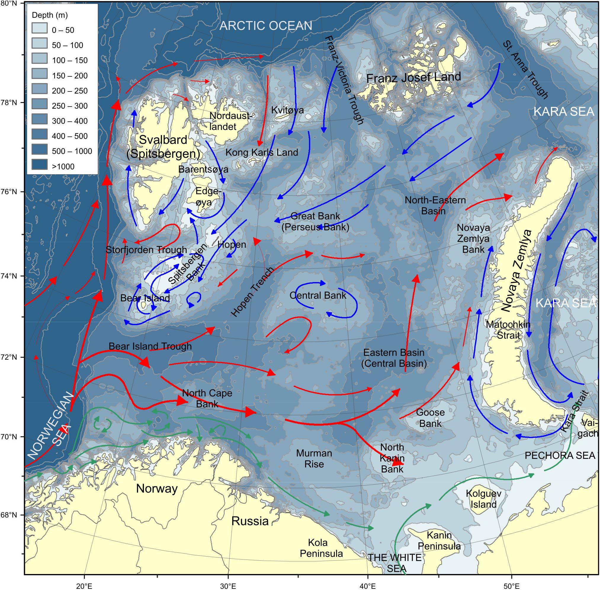
Figure 1. The Barents Sea. Red arrows show Atlantic water currents, blue arrows show Arctic water currents and green arrows show coastal currents. Depths are given in the legend.

Data Collection

Since 2004, the Joint Norwegian-Russian ecosystem survey (BESS) has provided near synoptic observations of physical and chemical oceanography, plankton, benthos, fish, seabirds, and sea mammals in August – September (Michalsen et al., 2011, 2013; Eriksen et al., 2018). The timing of the ecosystem survey in autumn allows access to most, or all, of the Barents Sea, as sea-ice is then at its seasonal minimum. At this time, the 0-group fish are large enough to be caught by pelagic trawl, while settlement to the bottom of the 0-groups of demersal species has not yet begun (Eriksen and Gjøsæter, 2013).

In 2016, the timing and coverage of BESS was not optimal due to lack of coverage of the central-southern area due to military exercises and an opposite direction of sampling (from north to south vs. from south to north as usual, ICES, 2017). The northern part of the Barents Sea was covered from 19. August to 2. September, the central part between 2. and 15. September and the southern parts between 15 and 30 September. Thus, the abundances of cod, redfish, herring and polar cod were underestimated and should be interpreted as minima (ICES, 2017).

A standard trawling procedure has been used on both Norwegian and Russian vessels. The standard gear, a small-meshed pelagic “Harstad” trawl with 20 × 20 m mouth opening, has been used to cover the upper water column (0–60 m) with the head-line at 0, 20, and 40 m (Eriksen et al., 2009). At each depth-level the trawl is towed for 10 min at a speed of 3 knots, corresponding to a towing-length of 0.5 nm or 0.93 km. Additional tows with the head-line at 60 and 80 m are occasionally made when dense concentrations of 0-group fish are recorded deeper than 60 m on the echo-sounder. During the cruise, pelagic catches were sorted, and the captured organisms identified to lowest possible taxonomic level.

Species-specific abundances of 0-group fish were estimated from each trawling event, using a standard procedure where number of trawl-depths, towed distance, opening area of the trawl, and trawl capture efficiency are taken into account (Eriksen et al., 2015, 2017). The 0-group fish abundances were given in millions of individuals per square nautical mile. Mean fish length per species was estimated for each trawl haul and given in centimeters. For 0-group fish, total fish length for 30 individuals (or all present in the catch when fewer) of each species were measured immediately after sorting the catch.

Jellyfish abundance was estimated on basis of each trawl haul by use of a standard procedure accounting for number of trawl depths, towed distance, and trawl opening area (Eriksen et al., 2012). Jellyfish of the species Cyanea capillata and Aurelia aurita were weighed separately. and their estimated abundances given in kg per square nautical mile.

Mesozooplankton in the Norwegian sector of the Barents Sea was collected by WP2 net with mouth-opening area of ∼0.25 m² (Fraser, 1966; Anonymous, 1968), while in the Russian sector a Juday net with mouth-opening area of ∼ 0.11 m² was applied. Both gears were rigged with nets of mesh-size 180 μm and hauled vertically from near the bottom to the surface. In this study, we use estimated mesozooplankton biomass (g dry-weight m^–2) representing the whole water-column. For the Norwegian sector, the samples were split into two halves, of which one was dedicated to estimation of biomass. Here the biomass was based on direct weight-measurements after drying in a cabinet at ca. 65°C for ca. 24 h (and repeated drying on shore before weighing), whereas for the Russian samples the biomass was estimated from wet-weight of formalin-fixed samples after removing excess moist with paper, and dividing by a factor of five for conversion from wet-weight to dry-weight. All weighing of samples, both from the Norwegian and Russian sectors, was performed on shore after the cruise.

Temperature and salinity were measured with CTD profilers from the surface to the bottom at the stations for trawling and net-sampling of plankton. CTD profiles were taken either before or after trawling, and in this study, we use temperature and salinity averaged over 0–50 m.

Data Analyses

Station-data collected during BESS in 2016 were used to investigate spatial distributions of both physical (0–50 m averaged temperature and salinity) and biological (species-specific 0-group fish abundances and lengths, mesozooplankton biomass, and jellyfish biomass) variables. The Barents Sea was divided into a grid with a resolution of 1-degree latitude × 2-degrees longitude. All observational positions were then assigned to the corresponding grid cell and average values of the different variables calculated, hence allowing for subsequent statistical analyses.

Abundances of all 0-group fish species in 2016 were compared with the long-term means (1980–2015) for the Barents Sea as a whole. Long-term time series were available for the seven most abundant species (herring, capelin, cod, haddock, polar cod, redfish, and long rough dab). The comparison of 2016 abundances vs. the long-term means were based on log_e (abundance + 1). Likewise, the average length of each species in 2016 was compared to the corresponding long-term average during 1980–2015 for the Barents Sea as a whole. Length-data were used untransformed. One-sample t-tests (two-tailed) were used to check if the abundance and mean length of each species in 2016 was significantly different from the long-term averages for 1980–2015 (average of the annual averages). Here the base package of the software environment R – version 3.4.2 (R Core Team, 2017) was used. Visualizations as well as statistical tests of 2016 abundances compared to the long-term averages were based on log_e(abundance + 1) transformed data, as the distributions of most species on normal scale were strongly skewed toward low values, becoming more symmetric and approaching the normal distribution after transformation.

For the spatially aggregated 2016 data, alternative transformations for fish abundance data were evaluated on basis of symmetry of distributions and potential outliers. Log_e(abundance + 1), with abundance representing estimated number of individuals per square nautical mile, was chosen as the transformation of 0-group fish in the multivariate statistical analyses. 0-group fish abundances were used both in unconstrained and constrained ordination, and in the latter case used as response variables.

The environmental data, comprising temperature, salinity, mesozooplankton biomass, jellyfish biomass as well as latitude and longitude of the sampling grids were checked with respect to distributions, potential outliers and collinearity. Based on this check, the environmental data were used untransformed in subsequent analyses. Collinearity among predictor variables in statistical analyses can be an issue, and was assessed by pairwise scatter-plots, Pearson correlation-coefficients, and the Variance Inflation Factor (VIF). Apart from average temperature in the 0–50 m layer being strongly and negatively related to latitude, collinearity among the environmental variables was not found to be problematic after excluding latitude (maximum correlations of | 0.4| and highest VIF below 1.6 for the rest of the variables).

Multivariate statistical analyses were made in the software environment R – version 3.4.2 (R Core Team, 2017) – and the package “Vegan” (Oksanen et al., 2019). The software Canoco version 5.11 (Šmilauer and Lepš, 2014) was also applied for multivariate statistics.

As a first step to reveal spatial structures in the data, a cluster-analysis was made including log-transformed 0-group fish abundances for all 8 species. Ward-clustering (method “ward.D2”), with Bray-Curtis distances was used (e.g., Greenacre and Primicerio, 2013). After inspecting the resulting dendrogram, we decided that the solution was to include 4 cluster-groups. For visualization, the locations of the grid-cells belonging to each cluster-group were plotted on a map.

Correspondence analysis (CA) (e.g., Greenacre, 1983; Legendre and Legendre, 2012; Greenacre and Primicerio, 2013) was performed on log-transformed 0-group fish data. Using the function “ordisurf,” supplementary (passive) environmental variables were superimposed as smoothed surfaces on the CA axes that were driven by the 0-group fish species. Note that these supplementary variables do not influence the ordination, and hence may only indicate relationships between the environmental variables and the species data. CA is an unconstrained gradient analysis that is based on unimodal species distributions (e.g., ter Braak and Šmilauer, 2012; Šmilauer and Lepš, 2014), and was applied to evaluate correlations among the species of 0-group fish while also considering spatial effects within the sampling area.

Canonical correspondence analysis (CCA) is a constrained multivariate ordination technique, which is a form of linear regression between two sets of variables, the response and predictor variables (e.g., ter Braak, 1986; Legendre and Legendre, 2012; Greenacre and Primicerio, 2013). CCA was run on the whole dataset that comprised both log-transformed 0-group species abundances (response variables) and selected non-transformed environmental data (predictor variables). The purpose of this was to perform statistical tests of the relationships between environmental data (mesozooplankton biomass, jellyfish biomass, and temperature) and the species complex of the 0-group fish. First, CCA was run using only one predictor variable at the time on the whole, original data set (N = 104 observations). To test the combined effect of the predictor variables, we applied forward selection by adding one environmental variable at the time. Finally, to account for spatial autocorrelation, spatially restricted permutation was applied on a reduced and rectangular dataset (N = 75 observations, within 18–48°E and 72–76°N). In this restricted dataset, cubic spline interpolation had been used to impute missing values in the central southern area.

Results

Long Term Mean vs. 2016 Situation

During the 1980s, abundance indices estimated for 0-group cod, herring, haddock and polar cod were low, while abundance indices for capelin and redfish were high. Cod, herring and polar cod abundance increased in the 1990s due to strong year classes of cod (1995–1997), herring (1996–1998), and polar cod (1991, 1994, 1996, and 1999), while abundances of capelin and redfish decreased (Figure 2).

FIGURE 2

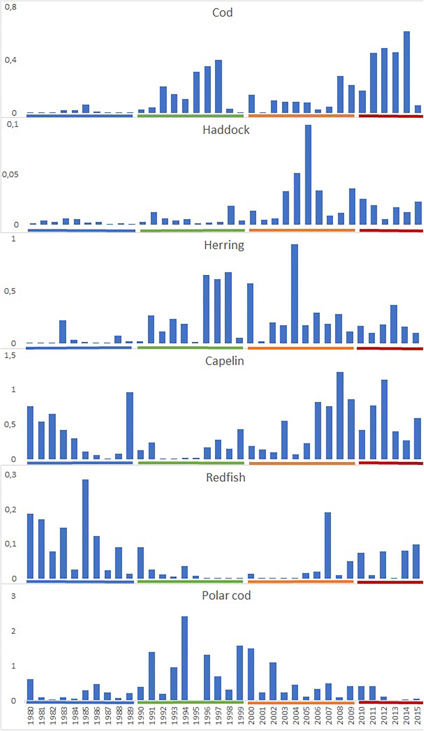
Figure 2. Annual total abundance (10¹² individuals) of 0-group fish of cod, haddock, herring, capelin, polar cod, and redfish between 1980 and 2015. Decades are indicated with colored lines (1980s – blue, 1990s – green, 2000s – orange, and 2010 – 2015 – red).

During the early 2000s, abundances of haddock, capelin and redfish increased, while abundances of cod and polar cod were rather low. During the last decade, abundances were especially high for cod and capelin, average for haddock, herring and redfish, while abundance of polar cod decreased dramatically (Figure 2).

The geographical distribution for 0-group fish (except redfish and polar cod) increased from the 1980s to the 2000s, and the size of the area occupied was associated with strength of the year classes (Figure 3, ICES, 2019). The geographical habitat of 0-group cod, redfish and polar cod was smaller in 2016 compared to recent years (2011–2015). In 2016, polar cod had almost disappeared in the core area of the southeastern Barents Sea. Further, in 2016 the densest aggregations of cod and herring displayed an eastward shift and that of and capelin a northward shift compared to the five preceding years (Figure 3).

FIGURE 3

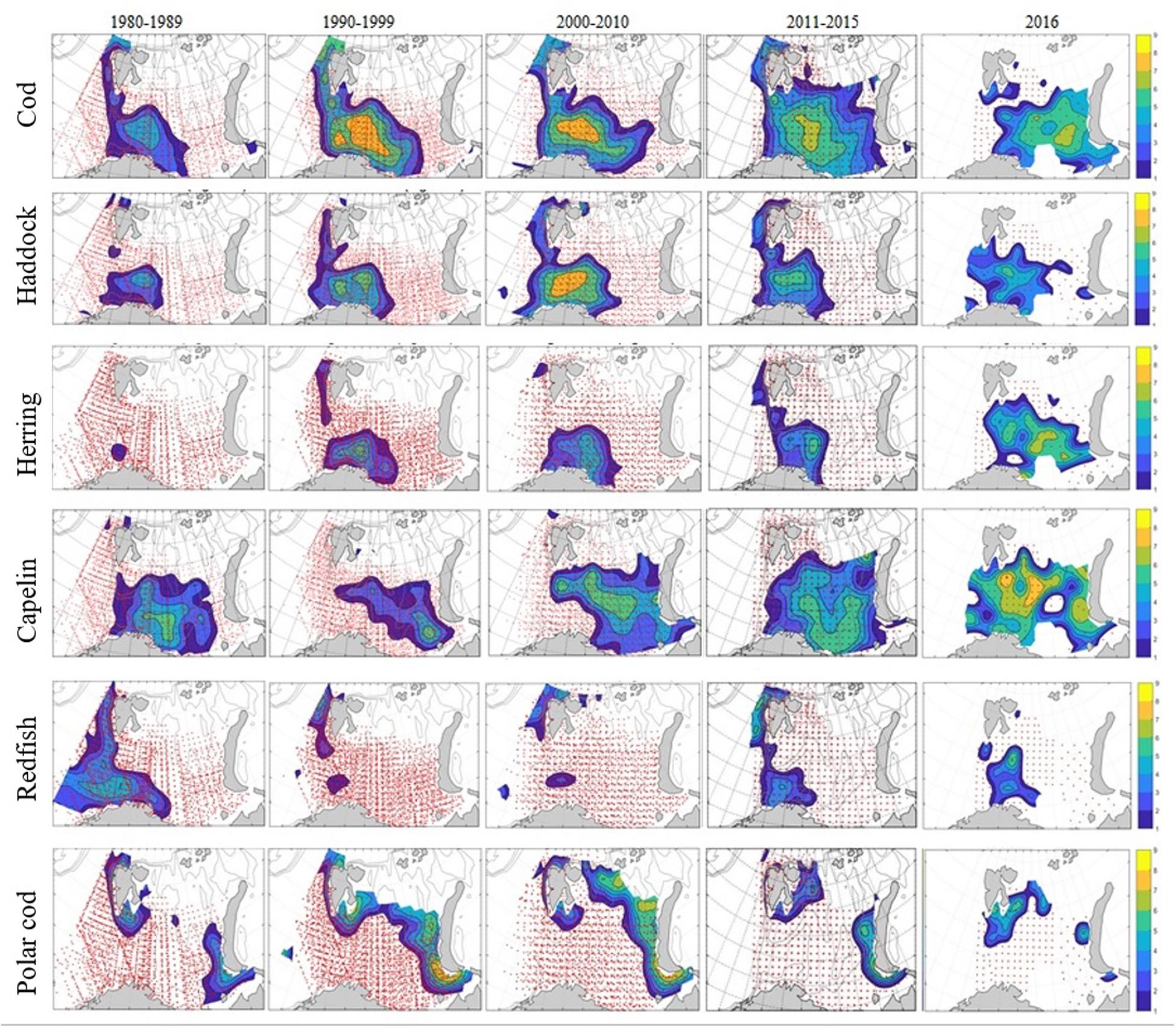
Figure 3. Distribution of 0-group fish in the Barents Sea during the 1980s, 1990s, 2000s, and 2010s. For comparison, distributions for year 2016 are shown in the column farthest to the right. Abundance estimates were log_e-transformed before mapping. Fish density varied from low (blue) to high (yellow). Red dots indicated sampling locations. Maps prepared for ICES 2019 and further publications.

Long-term time series (1980–2015) were available for the seven most abundant 0-group species (herring, capelin, cod, haddock, polar cod, redfish, and long rough dab). In 2016, the pooled abundance of these seven species was significantly and 35% higher than the long-term mean (1980–2015). The capelin-proportion of abundance in the pooled 0-group increased from 32% (long-term mean) to 80% (in 2016), the contribution from herring and haddock in 2016 was similar to the long-term mean, while the contributions from cod, redfish and polar cod were lower in 2016. Note that the timing and geographical coverage in 2016 differed from the surveys in earlier years, and thus fish abundance was underestimated (see M&M). The percentages reported above are based on abundances on normal scale.

In 2016, the observed fish abundance was significantly higher than the long term mean (1980–2015) for 0-group capelin, haddock, herring, and long rough dab, while not significantly different for cod and redfish (Figure 4). In contrast, polar cod abundance was significantly lower in 2016 compared to the long-term mean.

FIGURE 4

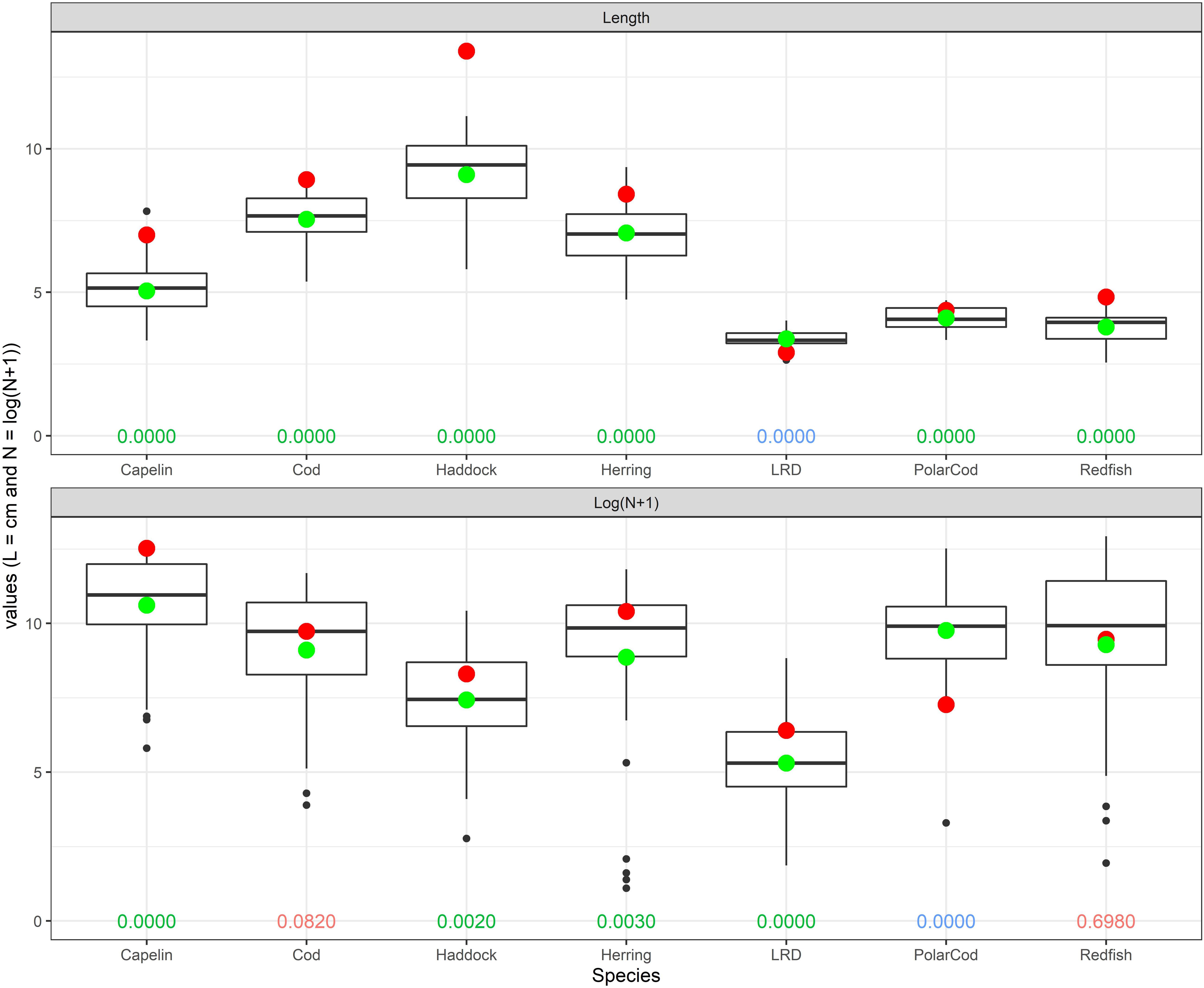
Figure 4. Upper: Average lengths for seven species in 2016 (red points) vs. the long-term average lengths for the years 1980–2015 (green points) for the whole Barents Sea. Data are on normal scale, and the 1980–2015 averages are based on the 36 annual values. Lower: Estimated total abundance of seven 0-group species during autumn 2016 (red points) vs. the 1980–2015 averages (green points) for the whole Barents Sea. All abundance data are shown as log_e(n + 1), and the 1980–2015 averages are based on the 36 annual values. The boxplots in the upper and lower panels encompass the 25–75 percentiles for annual means during 1980–2015, with the medians (50-percentiles) shown as thicker horizontal lines. The extending vertical lines indicate observations within 1.5 times the inter-quartile range from the upper or lower edge of the box, and circles show observations outside that range. Numbers along the bottoms of both figures give p-values for one-sample t-tests when comparing the abundance in 2016 with the average abundance for the years 1980–2015 both on log_e(n + 1) scale (upper panel) and average length in 2016 with the average length for the years 1980–2015 – on normal scale (lower panel). Green values indicate significant differences at the 5% level, with 2016 being higher than the long-term average. Blue indicate significant differences at the 5% level, with 2016 being lower than the long-term average, and red values denote that not significant at the 5% level.

In 2016, mean lengths were significantly higher for capelin (39%), cod (18%), haddock (47%), herring (19%), polar cod (7%), and redfish (28%). However, long rough dab was significantly shorter (14%) than the long-term average (Figure 4). The percentages refer to comparison with the long-term average.

Ambient Environment for the 0-Group Fish

In 2016, average temperature in the upper 50 m varied from 1.9 to 10.7°C with a mean value of 6.5°C. Warm Atlantic waters (T > 3°C) were found over a large area, and the northern region had colder water masses with temperature below 3°C in the upper 50 m (Figure 5). From southwest to northeast, the Barents Sea was covered by relatively saline water, and in the westernmost area salinity was as high as 35.1. Just southeast of Svalbard, and in the southeastern corner of the Barents Sea, waters were much fresher (salinity was close to 33).

FIGURE 5

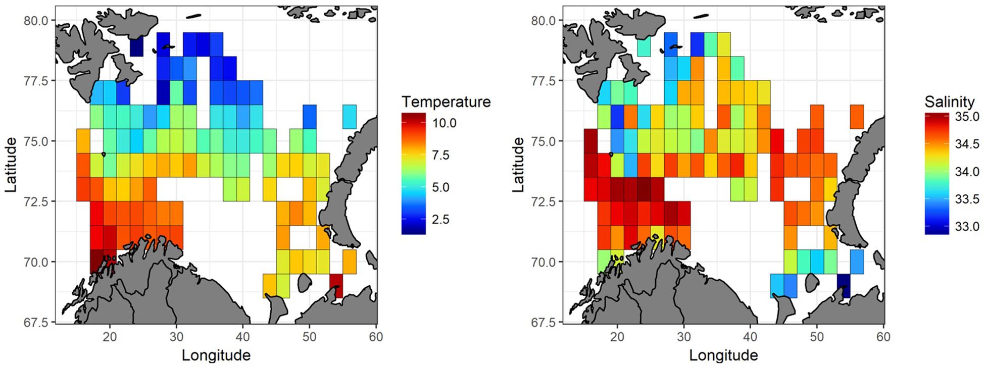
Figure 5. Barents Sea water temperature and salinity in the upper 50 m in August-September 2016. The lowest values indicated with blue color, and the highest with red.

In 2016, the average biomass of mesozooplankton was 5.9 grams of dry-weight m^–2 for the survey region as a whole, with the highest values (>15 g dry-weight m^–2) occurring mainly in the southwestern area. The jellyfish Cyanea capillata was widely distributed in the Barents Sea, with the highest abundances (>20 kg nmi^–2) in the northcentral area, and the lowest abundances (<1 kg nmi^–2) mainly observed in the western and northern areas (Figure 6). Copepods dominated in terms of abundance and large copepods (Calanus spp. which are prey for many young fishes, Dolgov et al., 2011) dominated in terms of biomass (ICES, 2017). The jellyfish Aurelia aurita was primarily observed close to the coast of the Norwegian and Russian mainland, and the abundance of this species was very low compared to that of C. capillata.

FIGURE 6

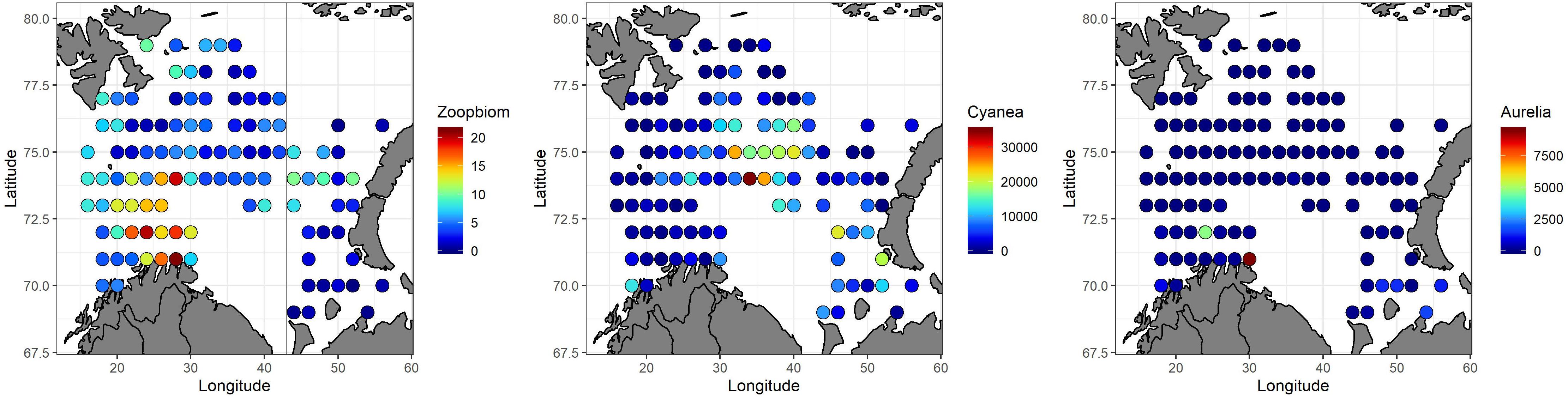
Figure 6. Spatial distributions of biomass for mesozooplankton (g dry-weight m^{– 2}, Russian station west of 43°E, left panel), the jellyfish Cyanea capillata (g wet-weight nmi², mid-panel) and the jellyfish Aurelia aurita (right panel, g wet-weight nmi^{– 2}) in 2016. The lowest values are indicated with blue color, and the highest values with red.

Abundances of 0-group herring, capelin, cod, haddock, polar cod, redfish, long rough dab and wolffish were gridded, and both richness (number of species present per grid cell – on normal scale) and total abundance of 0-group individuals (pooling all 8 species – on log-scale) are presented in Figure 7. Species richness was highest in the area southeast of Svalbard (the northwestern corner of the study-area), where all 8 species occurred. From this “species-hotspot,” the richness decreased with distance in all directions, and was generally lowest in the northern, eastern, southwestern and southeastern flanks of the survey area (Figure 7).

FIGURE 7

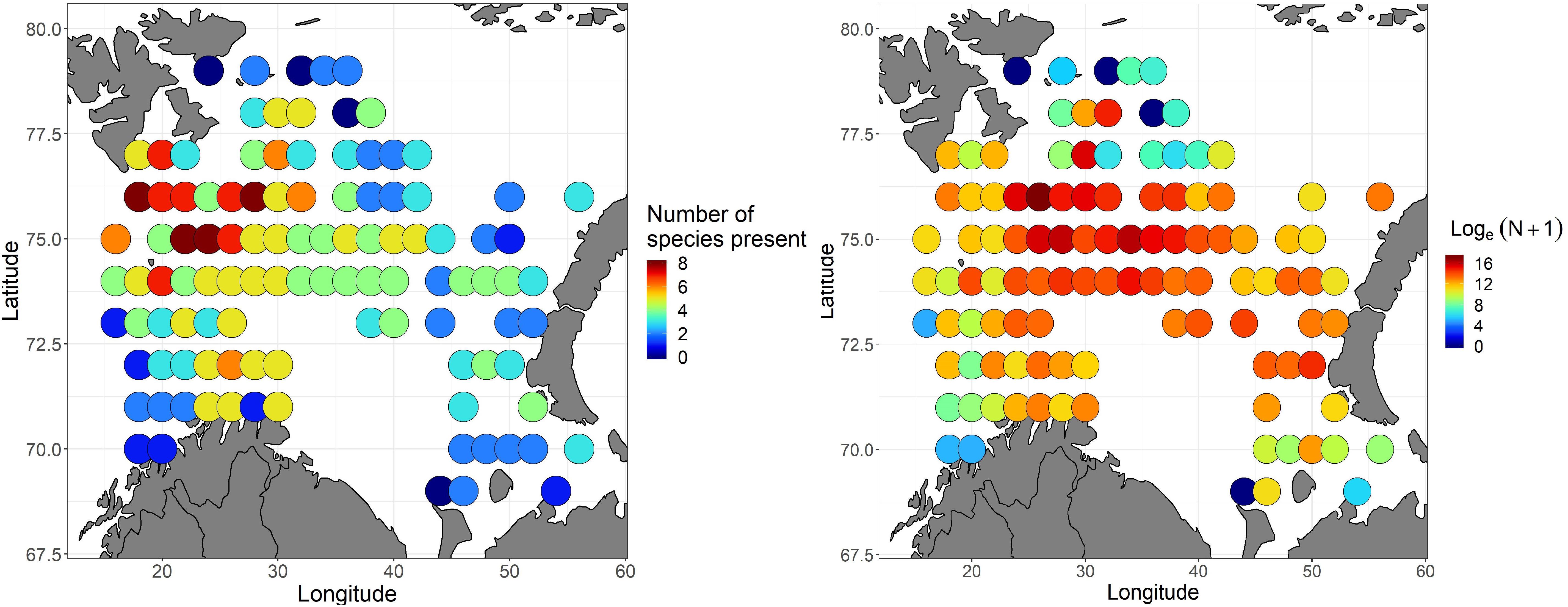
Figure 7. Left panel: Species richness in 2016 i.e., the number of 0-group fish species that were present per grid. Right panel: Log_e-abundance of 0-group fish (individuals per square nautical mile when pooling individuals of all 8 species; herring, capelin, cod, haddock, polar cod, redfish, long rough dab, and wolffish) in 2016. For both panels, colors indicate values, with blue representing the lowest and red the highest.

The highest concentrations of 0-group fish (all species pooled) were observed in the north-central Barents Sea, while the lowest concentrations were observed near the borders of the survey area (Figure 7).

0-Group Fish Abundance and Distribution

Capelin was the most abundant (mean abundance of 1.2 million individuals nmi^–2, when only including grids with capelin observations) and widest distributed 0-group fish species in 2016 (Figure 8). Herring, cod, and haddock were also widely distributed, though less abundant (mean abundances of 170, 62, and 23 thousand individuals nmi^–2, respectively, for grids where these species were observed). Cod displayed its highest abundances mainly in the northcentral and eastern areas, herring in the northcentral area, and haddock in the northcentral and south-western areas. Redfish (with mean abundance of 154 thousand individuals nmi^–2 for grids with occurrences) was distributed in the western area, while polar cod and long rough dab (with mean abundances of 24 and 11 thousand individuals nmi^–2, respectively, for grids with presences) occurred mainly in the northern and northwestern areas. Wolffish were generally confined to the northcentral region, with mean abundances of 305 individuals nmi^–2 for grids where this species was observed (Figure 8).

FIGURE 8

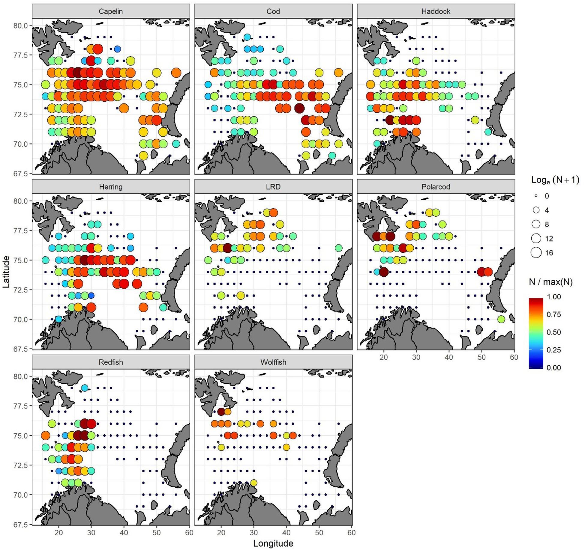
Figure 8. Spatial distributions of 0-group fish abundances (individuals nmi^{– 2}): capelin, cod, haddock, herring, redfish, long rough dab (LRD), polar cod, and wolffish in 2016. Black dots mark grid cells with no observation of a given 0-group species. Circle-size indicates log-abundance. Color indicates relative abundance within any given species – hence, color is not comparable for different species. Blue represents the lowest and red the highest relative abundances.

0-Group Fish Length

Mean fish length for capelin, cod, haddock, herring, long rough dab (LRD), polar cod, redfish, and wolffish for each grid is presented in Figure 9 and Table 1. Haddock was the largest 0-group fish, with an average length of 12.3 cm for the entire survey region. Haddock length varied between 7.5 and 15 cm, and the smallest fish were found in the northernmost area, while the largest occurred in the westernmost area (Figure 9). Cod, herring and wolffish were also relatively large with average lengths of 8.7, 7.8, and 7.6 cm for the entire region, respectively. The largest herring were found in the southern area, while the smallest – with a few exceptions – in the northern area. The largest cod were registered along the western border of the survey area. Despite wolffish occurring only within a limited area in the central Barents Sea, there seemed to be a tendency of the individuals being larger in the east (Figure 9). Capelin, redfish, polar cod and long rough dab were the smallest 0-group fishes, with average-lengths of 4.9, 4.4, 4.3, and 3.3 cm for the whole survey region, respectively. The largest capelin and redfish were found in the northern parts, and herring in the southern part of their distribution areas, while no clear patterns were seen for long rough dab and polar cod.

FIGURE 9

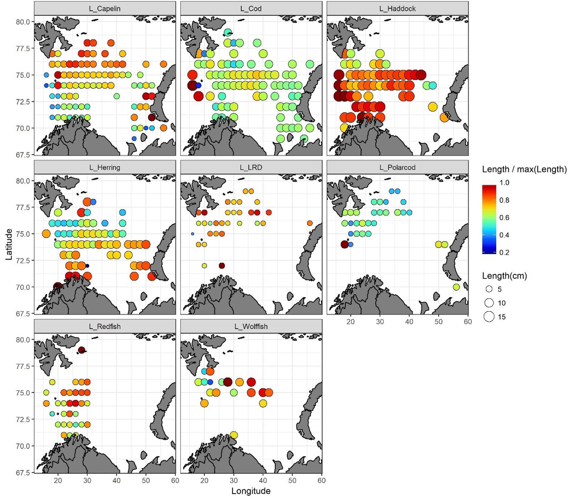
Figure 9. Spatial distributions of 0-group fish length for capelin, cod, haddock, herring, long rough dab (LRD), polar cod, redfish and wolffish in 2016. Circle-size indicates mean length (cm). Color indicates relative size within any given species – hence, color is not comparable for different species. Blue represents the shortest and red the longest fish.

TABLE 1

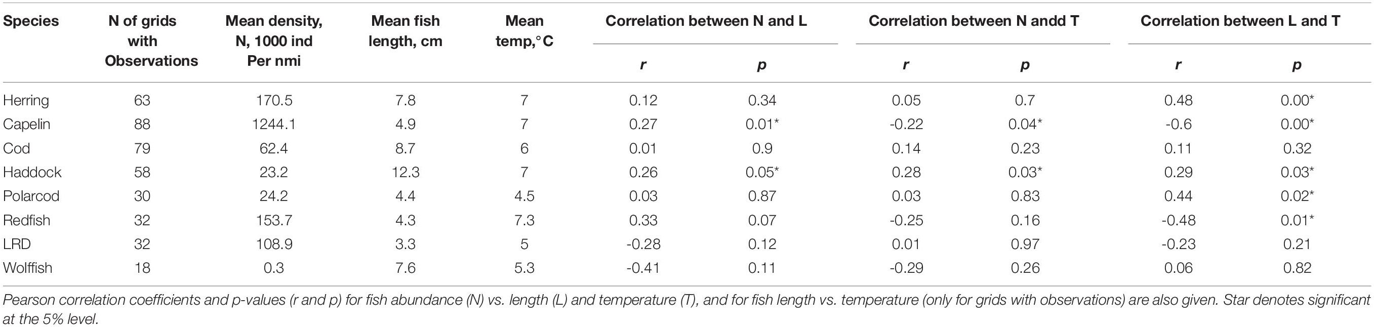
Table 1. Number of observations (grid cells of 1° in latitude × 2° in longitude, with total N of 108) for all 8 species; herring, capelin, cod, haddock, polar cod, redfish, long rough dab, and wolffish, along with mean fish-densities and lengths as well as mean temperature (only including grid cells with observations for these species).

Spatial Structure of 0-Group Fish

Cluster-analysis indicated spatial structure in the 0-group fish species composition, as shown when each grid was allocated to one of four categories (Figure 10).

FIGURE 10

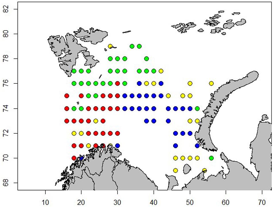
Figure 10. Spatial distribution of 4 clusters from Ward-clustering of abundance of 0-group herring, capelin, cod, haddock, polar cod, redfish, long rough dab and wolffish. Colors show different cluster groups. Cluster-analysis performed on log (abundance + 1) of each species, with abundance representing number of individuals per square nautical mile. Note that lengths of the 0-group fish were not included in the cluster analysis.

The red cluster was distributed in the western area and the fish community there was mainly represented by averaged sized capelin and large herring, haddock and redfish. The green cluster was located in the northern area and represented by mainly large capelin and smaller polar cod, long rough dab and wolffish. The blue cluster was found in the eastern area and was dominated by capelin of average size and cod of average size. The yellow cluster was dominated by smaller capelin and cod and displayed a more diffuse distribution (Figure 11).

FIGURE 11

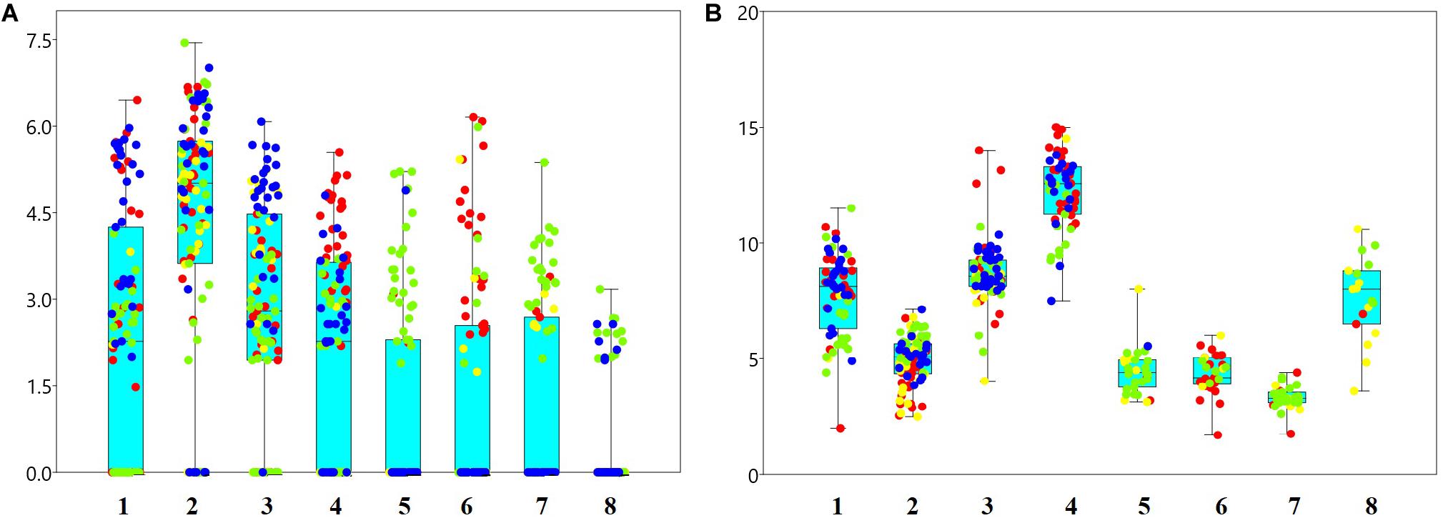
Figure 11. Log_e-abundances (A) and lengths (cm) for 0-group (B) herring (1), capelin (2), cod (3), haddock (4), polar cod (5), redfish (6), long rough dab (7) and wolffish (8). Colored dots show allocation to cluster – groups according to Figure 10, which indicated different areas: red dots – western area, green – northern area, blue – eastern area, and yellow – less clearly defined.

To evaluate if abundance could impact fish length, we tested the correlation between fish abundance and mean length at the grid level. Fish length and abundance showed a positive and significant correlation for capelin, a near-significant (p = 0.05) positive correlation for haddock, and for the other species non-significant correlations (Table 1). These results did not suggest high fish abundances limiting fish growth, as expressed by fish length in this study.

To evaluate if temperature could impact fish abundance and length, we tested correlations between ambient temperature and mean fish abundance and length at the grid level. Temperature was found to be negatively and significantly associated with both capelin abundance and length, and negatively and significantly associated with redfish length. Temperature was positively and significantly associated with abundance and length of haddock, length of herring and polar cod (Table 1). The remaining correlations were not significant at the 5% level

0-Group Fish Habitat and Interactions

The eight 0-group fish species considered together occurred within the temperature interval of 2–11°C. The highest species-specific fish densities were found within the narrower temperature intervals of 3–5°C (polar cod), 4–6°C (capelin and wolffish), 5–6°C (redfish), 6–8°C (cod and herring), and 6–9°C (haddock). Most of the 0-group fishes were distributed within their core thermal habitat, as established by Eriksen et al. (2012; 2015; 2.0–5.5°C for polar cod, 2.2–6.3°C for capelin, 4.4–8.0°C for cod, 5.2–8.7°C for herring, 4.1–10.5°C for haddock, and 5.5–8.5°C for redfish). However, abundant and large (>5 cm) polar cod were found in warmer water close to Novaya Zemlya (eastern Barents Sea), while abundant and smaller individuals (close to 3 cm) were observed near the Spitsbergen archipelago.

The largest 0-group fish were found within a temperature interval of 2–3°C and at 10°C (herring), 2–3°C and at 9°C (long rough dab), 2–5°C (capelin), 3–6°C (wolffish), 5–6°C and 8–9°C (cod), 5–7°C (redfish), close to 7°C (polar cod), and 9–10°C (haddock). Fish length was significantly correlated (both positively and negatively) with temperature, indicating that the larger fish were found in the areas with higher (herring, haddock and polar cod) as well as lower (capelin and redfish) temperatures (Table 1).

Correspondence analysis (CA) was performed on the log_e(abundances + 1) of the 0-group fish species, and environmental variables were superimposed passively as smoothed surfaces on the plots (Figure 12). The first axis (CA1) indicated a north-south gradient, while the second axis (CA2) an east-west gradient in the data (Figure 12), and these two axes, respectively, explained ∼38 and 20% of the total 0-group species variation. The CA plot shows that polar cod and long rough dab mainly occurred in the northern area, which was characterized by low water temperatures, low salinities, low plankton biomass as well as low levels of C. capillata (Figure 12). At lower latitudes, redfish and haddock were most common in the west and cod in the east. The CA indicated that redfish and haddock were associated with warmer and more saline waters, concurring with the highest biomass of mesozooplankton (Figure 12). Capelin, cod and herring were most abundant in the areas occupied by relatively warm waters with intermediate salinity, and with intermediate biomasses of mesozooplankton and relatively high concentrations of C. capillata. Wolffish was found primarily in the area with intermediate levels of most environmental variables (Figure 12).

FIGURE 12

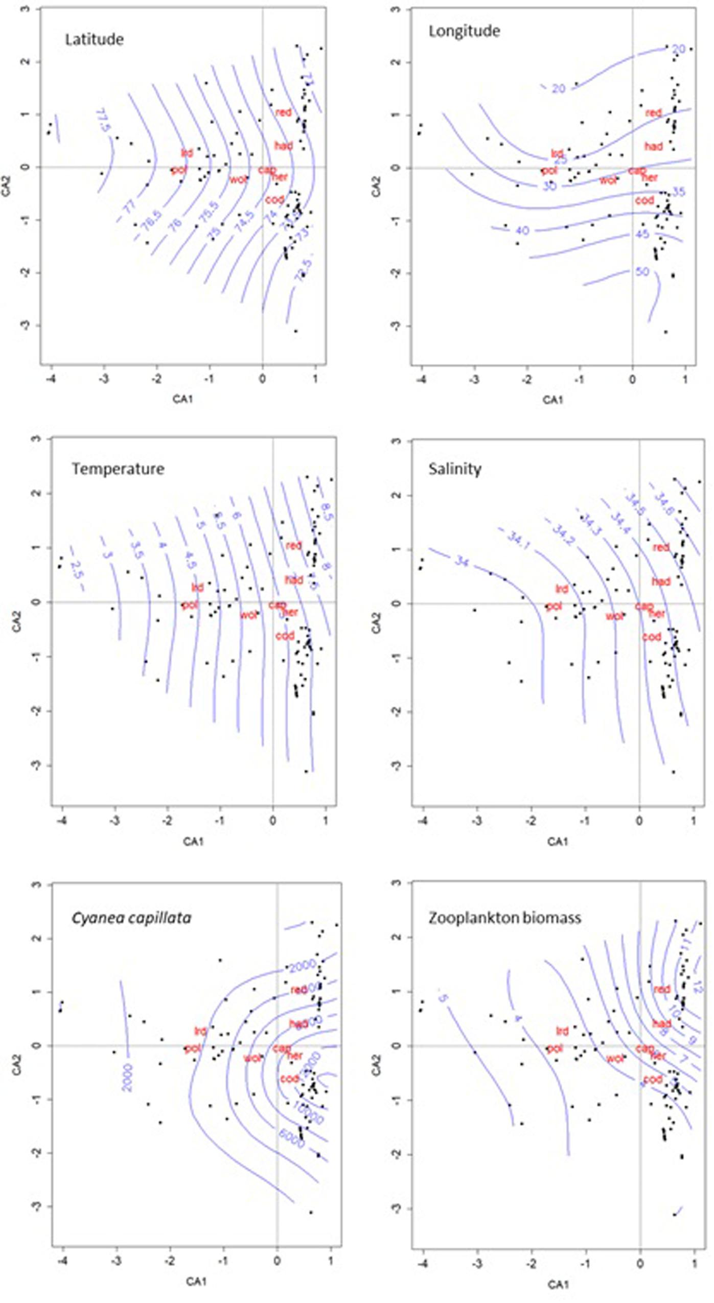
Figure 12. Triplots for correspondence analysis of log-abundance of 0-group fish species – herring (her), capelin (cap), cod, haddock (had), polar cod (pol), redfish (red), long rough dab (lrd), and wolffish (wol) (log individuals nmi^–2). Environmental variables passively superimposed as smoothed surfaces. Aurelia aurita is not shown as it was present only at a few stations.

Canonical correspondence analysis (CCA) was performed with log_e(abundance + 1) of 0-group fish species as response and environmental variables (0–50 m averaged temperature, biomasses of mesozooplankton and C. capillata) as predictor variables. Salinity (0–50 m) was correlated (p < 0.001, Spearmans rs = 0.41) with temperature 0–50 m, and therefore not used in the CCA. First the analysis was made on the original dataset with 104 observations (grids), using random permutations, and testing the effect of only one predictor variable at the time (Table 2). These three models and their predictors were all highly significant, although the model with temperature as predictor explained more of the variability than the other models (Table 2). Thereafter we ran models on the original dataset, first with two and then 3 predictor variables at the time (Table 2). All models combining two or three of the predictors (temperature, biomass of mesozooplankton, biomass of the jellyfish C. capillata) were highly significant, as were the different predictors (Table 2). The most complex model, including all 3 predictors, had the highest explanatory power, 31.6% (Figure 10).

TABLE 2

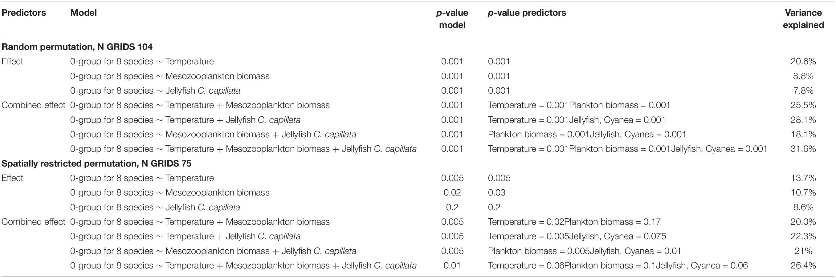
Table 2. Results of canonical correspondence analyses, first applying random permutations (104 observations) and then spatially restricted permutations (75 observations).

Finally, the analyses above were repeated using a reduced dataset with 75 regularly spaced observations (grids) where missing grids had been imputed by interpolation, and where spatially restricted permutation was used to account for spatial autocorrelations in the estimation of p-values. The statistical results resembled those of the original analysis but were generally less significant (Table 2). Depending on which other predictors that were included in a specific model, the effect of a given predictor could vary. We note that there was some collinearity between the predictors in this dataset, which can cause such effects. Considering the results for the different restricted permutation models along with the mentioned slight collinearity, the predictors temperature, biomass of mesozooplankton and biomass of the jellyfish C. capillata were all related to the variation within the 0-group fish complex – but with their significance depending on which other predictors that were included simultaneously.

The interpretation of the associations between the 0-group fish species abundances and the 3 environmental variables tested in the most complex CCA model (Figure 13) would be rather similar to that described above for the CA model fitted with supplementary (passive) environmental variables (Figure 9). For the CCA model shown in Figure 13, the first axis (CCA1) indicated a south-north gradient, and the second axis (CCA2) an east-west gradient. The CCA model also showed that capelin, herring, cod and haddock were generally associated with comparatively warmer waters and intermediate to higher abundances of plankton, while polar cod, long rough dab and wolfish were associated with colder waters. We also note that the CCA model for cod and herring suggested a positive relationship with C. capillata (Figure 13).

FIGURE 13

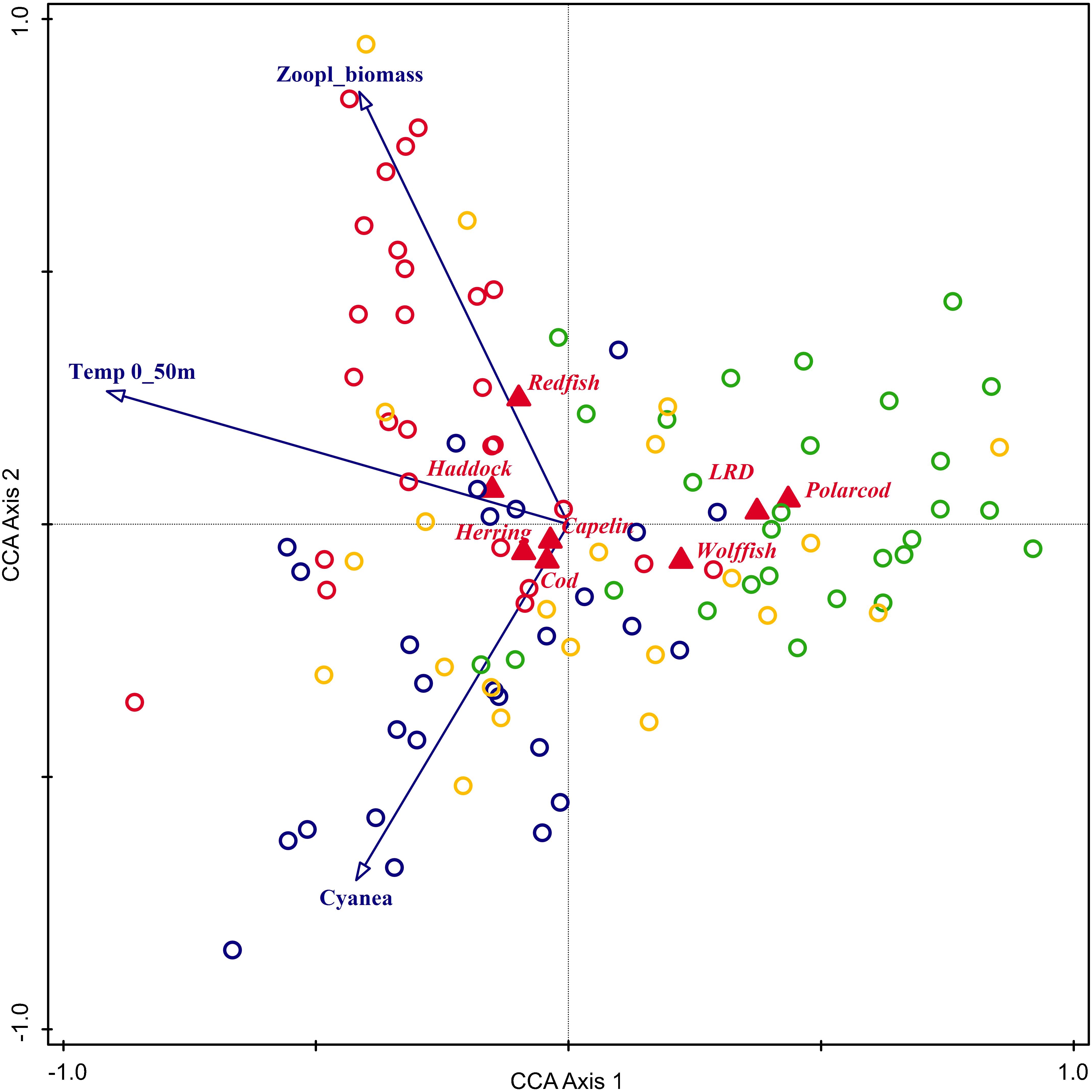
Figure 13. Triplots for canonical correspondence analysis (CCA) with abundance of 0-group fish species – herring, capelin, cod, haddock, polar cod, redfish, long rough dab (LRD), and wolffish (log millions of individuals per square nautical mile) as response and 0–50 m averaged temperature and biomasses of zooplankton and Cyanea capillata as predictor-variables. Response variables are shown in red, and predictor variables in blue. Grid-cells are colored according to their corresponding cluster groups – see Figure 10 for reference. This figure is based on the analysis using the original dataset consisting of 104 observations (grid cells).

Discussion

This paper focuses on one specific year with the aim of exploring how the record-warm conditions in 2016 influenced the Barents Sea 0-group fish distributions, abundances, and sizes. Our analyses of spatial distribution for 0-group fish (abundances and lengths) and their habitat indicated that larger individuals and higher abundances were observed mainly in the areas covered by relatively warm water masses (>3°C) apparently holding a sufficient amount of plankton. Even if 2016 was a record-warm year, most of the 0-group fishes were distributed within their thermal habitats, but with some shift of geographical habitat most likely reflecting a shift in the distribution of warmer water masses or lack of an adequate thermal habitat (polar cod in the south eastern area). In conclusion, the record warm temperature condition did not seem to limit the abundance and length for most of the 0-group fish species. The exception was polar cod, for which it seems that higher temperature, especially in the core area (eastern and southeastern Barents Sea), limited its distribution and abundance.

The Barents Sea ecosystem is dynamic and has been shown to undergo large fluctuations in response to climate variability at different time scales including multidecadal and interannual (Sætersdal and Loeng, 1987; Skjoldal and Rey, 1989; Loeng and Drinkwater, 2007). The pelagic compartment is directly and intimately connected to the ocean climate system and is expected to respond more rapidly to climate variability than for instance the benthic compartment (Rijnsdorp et al., 2009; Ottersen et al., 2010; Perry et al., 2010). Even small changes in temperature can directly influence the physiology and ecology of fish (Hochachka and Somero, 2001; Pörtner, 2001). Since around 1980, the Barents Sea has been on a warming trend with an increase of nearly 1.5°C and in the southeastern areas up to 2–3°C (ICES, 2017). The warming has been particularly high during the last three decades when we have seen record warm conditions and an increased pelagic biomass by a factor of two from around 11 million tones (1993–2003) to around 23 million tones (2004–2013, Eriksen et al., 2017), and an increase in 0-group biomass from 0.7 (1990s) to 2 million tones (2010s, ICES, 2018). The increasing water temperatures and changes in distribution of water masses and plankton communities have induced poleward shifts in the distribution of several boreal fish species (Ingvaldsen and Gjøsæter, 2013; Prokhorova, 2013; Fossheim et al., 2015). The decadal maps for the 0-group fish (see section Results) showed considerable changes in distribution patterns over last decades. Further, in 2016 the densest aggregations of cod and herring displayed an eastward shift and that of capelin a northward shift compared to the five preceding years. Spatial pattern of 0-group fish in the Barents Sea in autumn is complex and most likely reflects changes in the currents transporting the larvae but might also include effects of possible changes in location of spawning areas, or a combination of both. The stock size and structure can also have effects on the distribution of larvae through choice of spawning areas and total egg production. Differential mortality can alter distributions through good or poor survival of larvae in different parts of the transport and distribution areas.

0-group fish occupy the entire Barents Sea and overlap spatially with the older pelagic fishes (capelin, young herring, polar cod and blue whiting Micromesistius poutassou). 0-group fish primarily consume younger and/or smaller individuals of plankton forms like Calanus finmarchicus, other calanoid copepods, and euphausiids (Pedersen and Fossheim, 2008; Dalpadado et al., 2009; Prokopchuk, 2009), while adult pelagic fish prey mainly on larger individuals of these same taxa (Gjøsæter, 1998; Dalpadado et al., 2002; Prokopchuk, 2009). In August–September (end of the heavy feeding period) 2016, the highest mesozooplankton biomasses (>10 g m^–2) occurred in the southwestern region, hence only slightly overlapping with the high concentration area of 0-group species (herring, capelin, cod, haddock, and redfish) with longer individuals (herring, cod and haddock). Moderate biomasses of mesozooplankton (<7g m^–2) were observed in the northern and northcentral Barents Sea. The fish community there was characterized by abundant and large capelin, and relatively abundant and smaller polar cod, long rough dab and wolffish. Generally lower biomasses of mesozooplankton were observed in the eastern (<5g m^–2) and even lower in the southeastern (1–2g m^–2) Barents Sea, where large and medium sized cod, capelin and herring were observed. Autumn long-term monitoring of mesoplankton showed that biomass was generally lower (3 g m^–2) in the southeastern Barents Sea compared to the southwestern (7–11g m^–2) and the northern (5–10g m^–2) areas (1989–2016, ICES, 2018). Our results suggest that high fish abundances did not limit fish (age 0) growth, as expressed by fish length in this study. Furthermore, as exemplified by the multivariate models, the 0-group capelin, herring, and cod were mainly associated with intermediate, and haddock with relatively high mesozooplankton biomass. Therefore, the feeding conditions during summer and at the end of the feeding period (August–September) were indicated to be good for these species. However, for polar cod in the southeastern area, zooplankton biomass was low and most likely representing poorer feeding conditions then elsewhere.

In this context it is worth noting that with increasing temperature, ice retreat, and increased areas covered with Atlantic water and decreasing areas representing arctic waters, the Atlantic copepod C. finmarchicus will find the Barents Sea more hospitable and its arctic relative Calanus glacialis the opposite. Despite these sibling species typically co-occurring, C. glacialis is mainly found in the cold Arctic waters, in northern parts of the Barents Sea (Aarflot et al., 2017), where it can take advantage of ice-associated algae during parts of its life-cycle (Daase et al., 2013). Since C. glacialis is more lipid-rich than C. finmarchicus, there is a general concern that a change in the proportion of these two species in favor of C. finmarchicus, will affect individuals on higher trophic levels that depend on the energy-rich C. glacialis as food (Søreide et al., 2010). However, the autumn plankton community of the southeastern Barents Sea, the traditional core area of polar cod, is numerically dominated by the small species Oithona similis and Pseudocalanus sp. as well as the larger C. finmarchicus, while the biomass is generally dominated by C. finmarchicus and Metridia longa (ICES, 2017, 2018, 2019).

In August–September 2016, our results showed that the average temperature in the upper 50 m was 6.5°C, and that warm Atlantic waters (T > 3°C) covered a large area, and that only the northern area was covered by colder (<3°C) water masses. In 2016, Atlantic waters covered the largest observed area since 1965 (ICES, 2017). The 0-group fish were generally observed within the wide thermal interval – 1°C < T < 10.5°C (1980–2008, Eriksen et al., 2012). In 2016, 0-group fish species were found in the narrower temperature interval (2–11°C). The mean ambient temperature varied among the species and was lowest for polar cod and long rough dab and highest for redfish and haddock due to their geographic habitat. Most 0-group fishes were distributed within their core thermal habitat (defined for the period 1980–2008 by Eriksen et al., 2012), except for polar cod (see below). Even if the 0-groups were found within their thermal habitat, the distributional shift of water masses most likely influenced a shift in geographical habitat for 0-group cod, herring and capelin in 2016 compared to recent years. The multivariate analyses showed that 0-group capelin, herring, cod, haddock and redfish were mainly associated with the comparatively warmer water masses. It seems that a large area covered with relatively warm waters provided favorable living conditions for most of the 0-group fish in 2016.

In 2016, polar cod was distributed in two distinct areas: primarily southeast and east of the Spitsbergen archipelago. In the southeastern Barents Sea polar cod were found in two catches only. The component of polar cod experienced unusually high water temperature conditions with anomalies of 2.5–5°C due to unusually warm conditions over those shallow areas in 2016 (Trofimov and Ingvaldsen, 2017). Polar cod were found at temperatures of 6–7°C, significantly higher than their core thermal habitat at 2.5–5.5°C. Laurel et al. (2016) studied polar cod growth and swimming activities at different temperatures in the laboratory and found relatively high growth at 0°C and maximal growth at 7°C when food was abundant. Earlier, low abundance of large polar cod were found in the Barents Sea at temperature of 6–8°C (Eriksen et al., 2012). Thus, high temperatures and low zooplankton biomasses in 2016 may have limited the polar cod distribution and abundance in the core area. These findings are in agreement with earlier studies suggesting that further increases in temperature may lead to worse conditions for 0-group polar cod in the Barents Sea, in addition to other factors such as a reduced spawning stock and spawning areas and/or a poor feeding habitat (Hop and Gjøsæter, 2013; Eriksen et al., 2015; Huserbråten et al., 2019). In addition, feeding condition during the first summer may also influence the autumn abundance and distribution of polar cod.

In 2016, the survey started in the north, and thus the northern and north-central areas were covered approximately 1 month earlier than usual. Despite the early coverage, the length of 0-group capelin, cod, haddock, herring, redfish, and long rough dab were higher than the long-term mean. Larger fish observed in August–September may indicate good feeding conditions and fast growth during the first months of their life. However, comparatively large 0-group fish could also indicate earlier spawning and hence more time to grow. We have no information about spawning time in 2016 compared to other years for the fish species here studied. However, this might be the case for capelin, as the largest individuals were found close to the northern and eastern borders of their distribution, which is furthest away from the spawning areas along the northern Norwegian coast.

Abundances and spatial distributions of 0-group fish in autumn should primarily depend on where and when the individuals were spawned, the prevailing current patterns and strengths, as well as food availability, temperature and mortality rates. The plankton, including jellyfish, fish eggs and fish larvae, drift into the Barents Sea with the Norwegian Atlantic Current and the Norwegian Coastal Current and the strength of the inflow of Atlantic waters and its direction within the Barents Sea varies within years (Ozhigin et al., 2011). In 2016, in addition to the high abundance of 0-group fish, especially for capelin, relatively high biomasses of C. capillata (1.6 million tones in 2016, long-term mean of 1.2 million tones, 1980–2016) were registered (ICES, 2017). Our results, including the multivariate models, showed that the 0-groups of capelin, herring, cod and haddock were associated with intermediate to high abundances of C. capillata (Figure 12). High abundances of jellyfish can significantly impact the pelagic community, including the 0-group fish, through direct predation and competition for food (reviewed by Purcell, 1985) as well as through cascading effects (Lindahl and Hernroth, 1983; Schneider and Behrends, 1998; Pitt et al., 2009). Also a recent, spatial study from the Barents Sea further showed that abundances of the jellyfish, C. capillata, and 0-group herring, cod and haddock were positively related, indicating that they were inhabiting similar water masses in the Barents Sea (Eriksen, 2015). Even if we cannot estimate the predation impact of jellyfish on the fish larvae or 0-group, we assume that this might be important. Our spatial analysis showed that biomass of C. capillata was positively related to abundances of 0-group herring, capelin and cod, indicating that they were inhabiting similar water masses. This shows that relatively high abundances of this jellyfish had not reduced the 0-group fish abundances to levels where negative impacts were detectable.

Conclusion

In conclusion, we believe that the thorough description of the environmental conditions in the habitats for 0-group species presented in this paper will be useful to other studies dealing with time series analyses of fish recruitment, as well as modeling studies on future climate effects in the Barents Sea.

Data Availability Statement

The original contributions presented in the study are included in the article, further inquiries can be directed to the corresponding author.

Author Contributions

EE, EB, and ES were responsible for analyzing data, preparing maps, discussion, and writing the manuscript. EB and RP were responsible for multivariate analyses. AT, TP, and IP contributed writing the manuscript.

Conflict of Interest

The authors declare that the research was conducted in the absence of any commercial or financial relationships that could be construed as a potential conflict of interest.

Acknowledgments

We would like to acknowledge the financial support provided by the Barents Sea Research Program at IMR (projects “HAV/WGIBAR” and “Monitoring of plankton and trophic interactions in the Barents Sea”) and the Norwegian Ministry of Climate and Environment (project “BSECO”, QZA-15/0137) and “The Nansen Legacy” (RCN no. 276730).

References

Aarflot, J., Skjoldal, H.-R., Dalpadado, P., and Skern-Mauritzen, M. (2017). Contribution of Calanus species to the mesozooplankton biomass in the Barents Sea. ICES J. Mar. Sci. 75, 2342–2354.