 Paul E. Renaud1,2*
 Phil Wallhead3
 Jonne Kotta4
 Maria Włodarska-Kowalczuk5
 Richard G. J. Bellerby3,6Merli Rätsep4
 Dag Slagstad7Piotr Kukliński5
- 1Akvaplan-niva, Tromsø, Norway
- 2Department of Arctic Biology, The University Centre in Svalbard, Longyearbyen, Norway
- 3Norwegian Institute for Water Research, Bergen, Norway
- 4Estonian Marine Institute, University of Tartu, Tartu, Estonia
- 5Institute of Oceanology, Polish Academy of Sciences, Sopot, Poland
- 6SKLEC-NIVA Centre for Marine and Coastal Research, State Key Laboratory of Estuarine and Coastal Research, East China Normal University, Shanghai, China
- 7SINTEF, Trondheim, Norway
Arctic marine ecosystems are often assumed to be highly vulnerable to ongoing climate change, and are expected to undergo significant shifts in structure and function. Community shifts in benthic fauna are likely to result from changes in key physico-chemical drivers, such as ocean warming, but there is little ecological data on most Arctic species to support any specific predictions as to how vulnerable they are, or how future communities may be structured. We used a species distribution modeling approach (MaxEnt) to project changes over the 21st century in suitable habitat area for different species of benthic fauna by combining presence observations from the OBIS database with environmental data from a coupled climate-ocean model (SINMOD). Projected mean % habitat losses over taxonomic groups were small (0–11%), and no significant differences were found between Arctic, boreal, or Arcto-boreal groups, or between calcifying and non-calcifying groups. However, suitable habitat areas for 14 of 78 taxa were projected a change by over 20%, and several of these taxa are characteristic and/or habitat-forming fauna on some Arctic shelves, suggesting a potential for significant ecosystem impacts. These results highlight the weakness of general statements regarding vulnerability of taxa on biogeographic or presumed physiological grounds, and suggest that more basic biological data on Arctic taxa are needed for improved projections of ecosystem responses to climate change.
Introduction
Ongoing climate change affects multiple environmental drivers, with direct and indirect implications for marine ecosystems. For example, reductions in sea-ice volume and extent, increasing air and sea-surface temperatures, and freshwater and biogeochemical discharge in the Arctic have already been noted to be occurring at rates higher than the global average (IPCC, 2014; AMAP, 2017) with consequences for regional ocean acidification rates (Bates et al., 2012; Bellerby, 2017). Anthropogenic impacts from fossil fuel CO2 emissions are linked with changes in these drivers and have led to changes in ocean chemistry. These impacts include reductions in both ocean pH and carbonate mineral saturation states, which have been implicated in decreased performance of many marine taxa (Pörtner, 2008; Kroeker et al., 2011). Models project that ongoing ocean acidification (OA) will continue over the coming decades, and the degree of OA will be dependent mainly on social and policy decisions (e.g., Bellerby et al., 2014, 2018). The amplification of both warming and acidification observed in the Arctic, in combination with other expected physical and biological impacts, has led to the common viewpoint that Arctic ecosystems are particularly vulnerable to on-going climate changes (Smetacek and Nicol, 2005; Renaud et al., 2007; Brierley and Kingsford, 2009; Doney et al., 2012; Hoppe et al., 2018). Changes in community composition that may result are not merely of academic interest: they may reflect underlying functional responses with broad-reaching implications for ecosystem processes and services.
Laboratory experiments and field sampling have generated numerous but often contradictory predictions of how changes in climate-change-related drivers will affect marine life, from individuals to ecosystem processes. Physiology, phenology and life-history, community structure, and system productivity (Pörtner et al., 2005; Ardyna et al., 2014; Renaud et al., 2015, 2018) are just several examples of impacts that may be felt: from the very basic processes of life to the provisioning of ecosystem services. Until now, however, most studies have focused on effects of single factors, and usually in laboratory or isolated field settings (Pedersen et al., 2016; AMAP, 2018). Recent syntheses have called for investigations of broader thematic and spatial scope, including studying multiple factors in combination for arriving at more realistic predictions (e.g., AMAP, 2018), and adopting a pan-Arctic perspective when identifying trends in ecosystem response (Wassmann, 2015). These perspectives are needed for developing mitigation, adaptation, and management strategies for marine ecosystems across the Arctic (Halpern et al., 2012). Whereas some Arctic taxa are clearly threatened by changing climatic conditions (Kovacs et al., 2011; Doney et al., 2012; Grebmeier, 2012; Beaugrand and Kirby, 2018), a multi-factor investigation of vulnerability of Arctic taxa in general has not been performed.
One of the most intuitive changes that could be expected due to climate warming is the poleward expansion of boreal organisms. This has already been observed for both benthic and pelagic organisms, and is suggested to be largely related to thermal tolerance (e.g., Wethey and Woodin, 2008; Sunday et al., 2012; Neukermans et al., 2018). Indeed, dominance of boreal and Arctic taxa in seafloor (benthic) communities of the Barents Sea have been shown to fluctuate with temperature in the region over the past 100+ years (Blacker, 1965; Matishov et al., 2012). Niche theory is useful for making predictions as to historical or future distributions in the context of climate change. Single-variable models (thermal-envelope models) have been used to predict, for example, changes in fish distribution with climatic warming (Cheung et al., 2009). In Arctic systems, this technique is problematic due to high uncertainty in either fundamental or realized niches of nearly all taxa in the ecosystem. On-line databases can provide one way around this problem by identifying the characteristics of an organism’s realized niche. This technique has been used to identify benthic taxa that may expand or contract under warming scenarios (Renaud et al., 2015). Although biased by the geographical range of data included in databases, and non-random sampling in general, the method can also provide information for multi-dimensional realized niches. Once current distributions are mapped, a suite of species distribution models may be applied to project future distributions in response to multiple environmental drivers. Such modeling activities have been identified as critical next steps in understanding climate change effects on benthic community structure in Arctic environments (Renaud et al., 2015).
A key requirement for implementing these models is a well resolved and validated hydrographic/ocean chemistry model with realistic climate forcings. This allows for accurate physical characteristics to be assigned to each sampling location in both hindcasting and forecasting modes. One such model has recently been expanded to include the needed spatial and temporal perspectives for the carbonate system, and has been used to upscale results of a mesocosm experiment to other Arctic areas (Bellerby et al., 2012).
This study investigates the vulnerability of benthic fauna found in the Arctic and its marginal seas to end-of-century climate change. We use outputs from a state-of-the-art ecosystem model to drive species-distribution modeling for a broad range of characteristic macro- and mega- benthic taxa characteristic of the Arctic’s shelf seas. We analyse results to determine if Arctic taxa are more susceptible to changes in a combination of environmental drivers than boreal or more widespread taxa. We also investigate whether calcification status or higher taxonomic classification (phylum, class) could indicate vulnerability. Implications of the presence or absence of such patterns are discussed.
Materials and Methods
Environmental Projections
We ran the ocean biogeochemical model SINMOD (Slagstad et al., 2011, 2015), which includes a CO2 system module (Bellerby et al., 2012), to estimate bottom water temperature and aragonite saturation state (Ω(ar)). The SINMOD domain is pan-Arctic (see Figure 1) with 20 km horizontal grid resolution and 25 fixed depth levels, and calculations were based on biweekly saved output. Saturation state describes the seawater concentrations of carbonate and calcium ions relative to the equilibrium concentrations for that mineral; conditions near or below saturation (Ω = 1) are generally considered unfavorable for production or maintenance of normal calcification. SINMOD was first run to produce a hindcast simulation (1979–2008), and then to produce a projection (2001–2099) under the SRES (Special Report on Emissions Scenarios) scenario A1B (see Slagstad et al., 2015; Wallhead et al., 2017, for more details). SRES A1B is a mid-range business-as-usual scenario assuming a “balanced” use of fossil vs. non-fossil energy sources (Nakicenovic et al., 2000) that results in end-of-century global responses that are comparable to the more recent RCP6.0 scenario and substantially more conservative than the SRES A2 or RCP8.5 scenarios (Collins et al., 2013). SINMOD bottom-water output was corrected using bias estimates, calculated as a function of spatial position (temperature) or of model bathymetry (Ω(ar)) using a compilation of in situ observations and matched model output (see Wallhead et al., 2017). Water depth over the SINMOD grid was estimated by interpolating high-resolution bathymetry products (the 500 m resolution IBCAOv3, Jakobsson et al., 2012, where available, otherwise the 2 min ETOPOv2, National Geophysical Data Center, 2006).
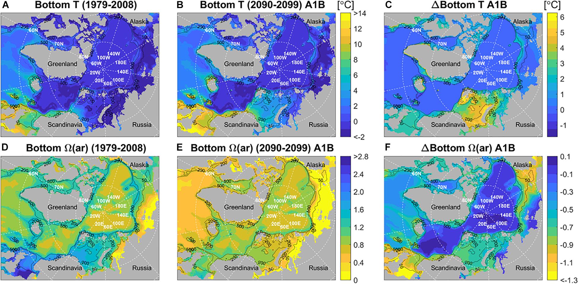
Figure 1. Bias-corrected SINMOD hindcasts and projections for bottom water temperature (A–C) and bottom water aragonite saturation state (D–F) under SRES A1B scenario. Left and middle figures show averages over the hindcast period (1978–2008) and the projection period (2090–2099), respectively; figures on the far right show the differences. Black lines show 50, 200, and 500 m depth contours.
Niche Description and Climatic Change
Occurrence records for 95 benthic taxa characteristic of Arctic shelf infaunal and epifaunal communities were extracted from the Ocean Biogeographic Information System database (OBIS1; extracted February 14, 2017; Supplementary Table S1). We chose taxa that were common, ecologically relevant (e.g., ecosystem engineers) and/or characteristic taxa of Arctic shelves, and where biogeographic affinities are well-known (see below). In addition, taxa were chosen to cover the range of factors studied here (biogeographic affiliation, calcification status, and higher taxonomic level). Further, we required that each taxon have at least 30 records within the geographic domain of SINMOD in order to maintain MaxEnt model performance and confidence level. This cutoff appeared to be sufficient since the model performed quite well for taxa with close to 30 observations (e.g., Parastichopus tremulus and Serripes groenlandicus, see Supplementary Tables S2, S3). Bottom water temperature and aragonite saturation state from the bias-corrected SINMOD hindcast output were matched to the georeferenced benthic fauna distributional records by interpolating from the model grid to the faunal data positions and averaging over the 5 years preceding each faunal observation date. Water depth at the sampling points was mostly (61%) from measurements when plausible values were provided; the remaining 39% were estimated using the high-resolution bathymetry products. Each species was assigned status as calcifying or not, biogeographic affinity (Matishov et al., 2012; World Register of Marine Species)2, and higher taxonomic grouping (mollusk, echinoderm, polychaete, crustacean, bryozoan).
In locations where species data have been collected systematically, for example through biological monitoring, both presence and absence of species at each site have been recorded. However, most observations of the OBIS database have been collected non-systematically and are available as presence-only records, and the different gear types deployed and study foci make it difficult to infer absence data from these records. We therefore employed a species distribution modeling approach that requires only presence data, in order to maximize the utility of the database.
From the water depth, temperature, and aragonite saturation state associated with each species record, we estimated three-dimensional realized niches and related them to the projected changes in these parameters through the end of the century. The contribution of each environmental variable to species occurrence probabilities in the Arctic was calculated using the MaxEnt method. MaxEnt is a machine-learning algorithm for modeling species distributions from presence-only species records. In brief, MaxEnt identifies the environmental characteristics of locations with species occurrences that differ from the environmental setting across the whole geographical region of interest. Based on the observed mismatch, a species’ suitable habitat is defined. More specifically, the MaxEnt model minimizes the relative entropy between two probability densities (one estimated from the presence data, and one from the landscape) defined in covariate space compared to a uniform distribution null model (see Merow et al., 2013 for details). MaxEnt’s predictive performance is consistently competitive with the highest performing methods. Since becoming available in 2004, it has been utilized extensively for finding correlates of species occurrences, mapping current distributions, and predicting to new times and places across many ecological, evolutionary, conservation and biosecurity applications (Elith et al., 2006).
Sampling Biases
By default, MaxEnt models assume that: (1) all locations on the landscape (or “background locations”) were equally likely to be sampled, and (2) any focal species would have been recorded at the sampled landscape points if it had actually occurred there. Assumption (1) is likely violated in our occurrence datasets, because of logistical and practical constraints on sampling in the Arctic (e.g., due to ice cover). Given such spatiotemporal biases, one cannot differentiate whether species are observed in a particular environmental niche because those locations are preferable or because they receive the largest search effort. Therefore, in order to relax assumption (1), landscape points were only drawn from the “target group sampling” (TGS) locations, which we defined as the total set of sampled locations for all species. However, this does not relax assumption (2), which may be violated where sampling gear and study focus have excluded certain species (Phillips et al., 2009). In theory the gear/study focus biases could be accounted for by partitioning the TGS, but this was not considered feasible for our particular dataset due to insufficient samples.
Model Fitting and Validation
Multicollinearity can be an issue with MaxEnt when answering if and when environmental variables are of ecological interest. Thus, prior to modeling, a correlation analysis was conducted for environmental variables and the final MaxEnt models included variables that were not significantly correlated with each other at p < 0.05 (aragonite saturation state, temperature, water depth). Calcite saturation state was excluded as it correlates highly with aragonite saturation state.
In this study MaxEnt models were fitted as combinations of basic functions and features. MaxEnt had six feature classes: linear, product, quadratic, hinge, threshold, and categorical. Products were all possible pairwise combinations of covariates, allowing simple interactions to be fitted. Threshold features allowed a “step” in the fitted function, hinge features were similar except they allowed a change in gradient of the response. Many threshold or hinge features were fitted for one covariate, giving a potentially complex function. Nevertheless, the MaxEnt program was allowed to simplify the associations between species and the environment and in many models only one or a few features were used, e.g., hinge, linear, and quadratic.
Segment-based (non-gridded) data were modeled using SWD (samples-with-data) format in MaxEnt for both presence and background sites. A separate model was run for each species. A 10-fold cross-validation was used to obtain out-of-sample estimates of predictive performance and estimates of uncertainty around fitted functions. In order to reduce model overfitting, a balance between accurate prediction (model fit) and generality (model complexity) was sought by maximizing the penalized maximum likelihood function, i.e., the gain function. When doing so, regularization or the LASSO penalty was applied by exploring a range of regularization parameter values and choosing a value that maximizes measures of fit on a cross-validation data set. The LASSO penalty is based on the rationale that features with larger variance should incur a larger penalty and, thus be less likely to be included in the model (Hastie et al., 2009). For model validation a random selection of 25% of the overall localities of species occurrences were used. The percent contributions of individual variables to the final model were identified with jackknife tests. The jackknife test evaluates how each variable contributes to the “gain” of the MaxEnt‘s model (i.e., improvement in penalized average log likelihood compared to null model) (Elith et al., 2011). We used the raw output (default) as this output is the closest estimate of the probability that the species is present (Elith et al., 2011).
Model Performance and Predictions
We used the area under the receiver-operating-characteristic curve (AUC) as a single measure of overall model accuracy that is not dependent upon a particular threshold. The value of the AUC is between 0.5 and 1.0 with AUC = 1.0 indicating that the model has a perfect match and AUC = 0.5 indicating that model is no better than random (Fielding and Bell, 1997).
The MaxEnt model was used to predict suitable habitat for each species under current and future environmental conditions, and differences between these predictions were used to assess the response to climate change of potential habitat area for each species. We are aware that projecting future species distributions usually involves extrapolating models to novel combinations of environmental variables, and such projections should be treated with extreme caution. However, a comparison of current and future environmental niche space indicated that only 20% of the whole study area would enter a completely novel environment, as defined by moving beyond the 3D convex hull of the present-day niche space distribution. We therefore consider any artifacts of extrapolation will have only a minor effect on our results.
Statistical Analyses of Model Results
Change in suitable habitat area from the present (1978–2008) to the future (2090–2099) was calculated from the MaxEnt model for each taxon. One-way analyses of variance (ANOVA) were performed for each of the three factors [calcification (as a t-test), biogeography, higher taxonomic level] on the change in habitat area (both percentage and absolute) after testing for homogeneity of variances and normality among factor levels (in each case these results were non-significant). Since single-factor analyses may obscure interaction effects or even effects of one factor when effects of a second factor dominate the variability, we also ran a 3-factor ANOVA on the data. Since we lacked degrees of freedom to run a fully factorial test, we used a main-effects model. Analyses were performed in Statistica v. 13.
Results
Environmental Settings Projections
Projections for bottom water temperature (T) and aragonite saturation state (Ω(ar)) indicate substantial changes over the 21st century (Figure 1). The warmer Atlantic Water-influenced zone expands northward and eastward from its current core in the southern and southwestern Barents Sea (Figures 1A,B), and benthic habitat in the Barents Sea warms by up to 6°C between 1979–2008 and 2090–2099 (Figure 1C). Over the same period, bottom Ω(ar) on the shelves (<500 m depth) decreases, mostly by 0.6–1.1 units from around 1–2 (weakly saturated) to 0–1 (undersaturated) (Figures 1D–F). Exceptions include the shallow Russian shelf regions (<50 m depth), which are already strongly undersaturated (Ω(ar) < 0.4; Figure 1D) and cannot become much more undersaturated in the future (Figures 1E,F). The largest decreases in Ω(ar) (∼1 unit) are in the North, Bering, and Chukchi Seas, and on the East Siberian Shelf at ∼50–500 m (Figure 1F). Arctic water-dominated areas of the northern and eastern Barents/Kara Seas remain relatively stable in temperature (Figure 1C), but experience Ω(ar) reductions as large as in the central Barents Sea (Figure 1F). Deeper areas (>500 m) in the Arctic and North Atlantic basins, and in Baffin Bay, see relatively small changes in benthic environment (Figures 1C,F).
Depicting Realized and Predicted Niches of Benthic Taxa
Of the 78 taxa with sufficient (>30) records for evaluation, the mean change in suitable habitat was small: approximately a 5% loss in suitable habitat based on MaxEnt. The range, however, was high, from a 42% increase in habitat (the amphipod Byblis gaimardii) to a 53% decrease (the sea cucumber P. tremulus) according to the 3-variable model (Table 1, Supplementary Table S2, and Figures 2, 3). MaxEnt performed very well for most (∼70%) taxa, with AUC > 0.9 (Supplementary Table S3). Temperature contributed most to defining the niche space for 72% of the taxa, while depth and aragonite saturation state were the largest contributors for 19 and 8% of the taxa, respectively (Supplementary Table S3).
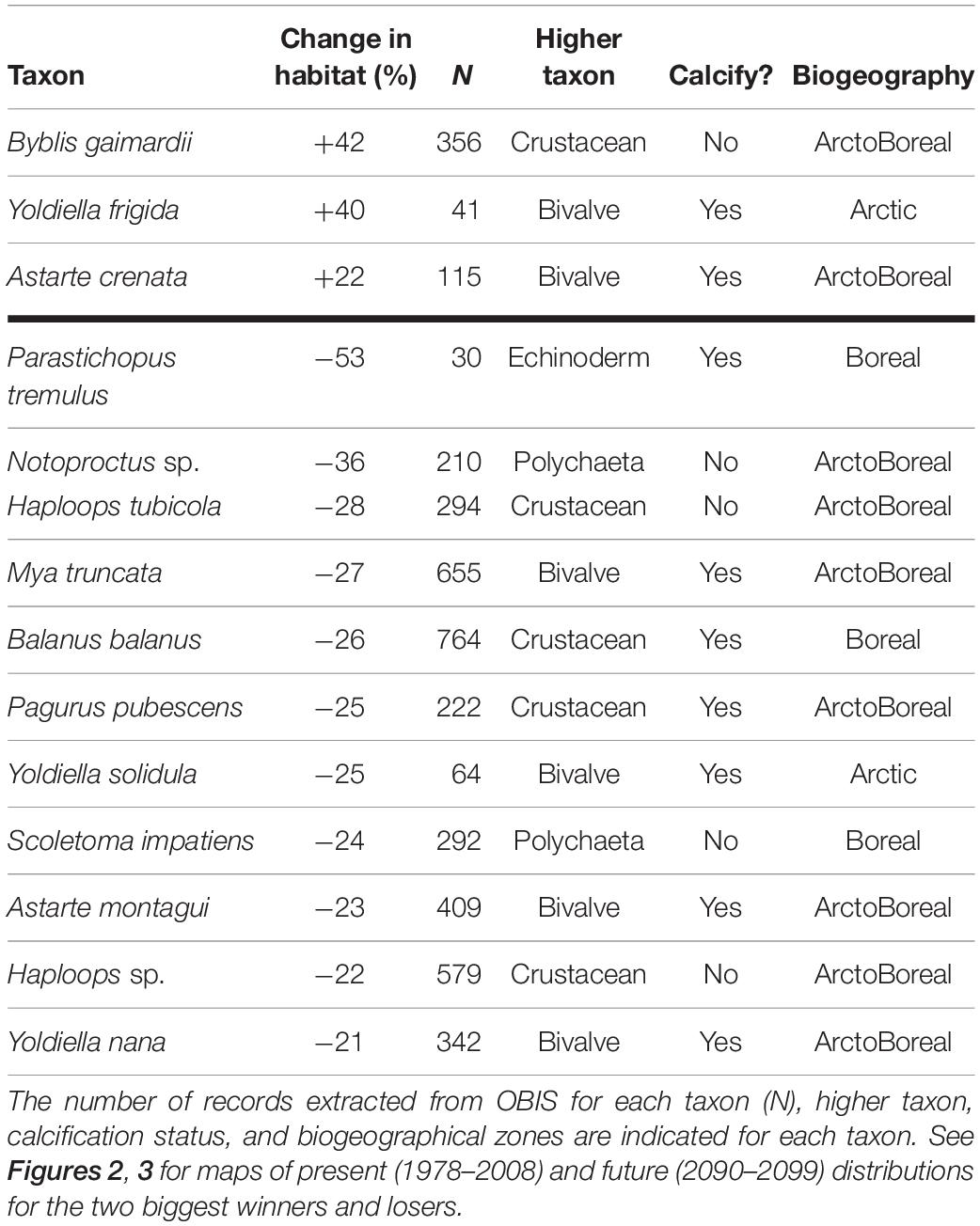
Table 1. Winners (>20% increase in suitable habitat, upper panel) and losers (>20% decrease in suitable habitat, lower panel) as predicted by the MaxEnt model.
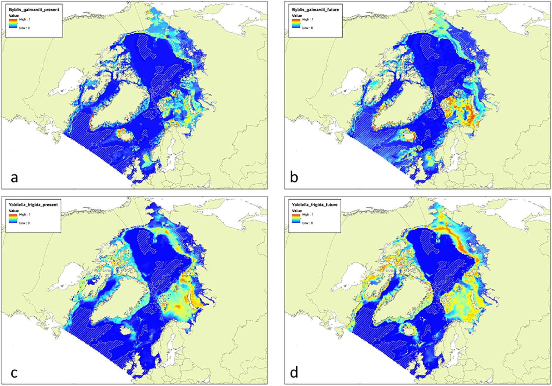
Figure 2. Habitat suitability maps for the two biggest winners [the Arcto-boreal amphipod Byblis gaimardii (+42%): (A,B); and the Arctic bivalve Yoldiella frigida (+40%): (C,D)] in the study area based on the results from the MaxEnt model (see Table 1). Maps show present (A,C) and predicted future (B,D) distributions for the two species. All models predict the expected probability of occurrence from 0 (0% probability; blue) to 1 (100% probability; red).
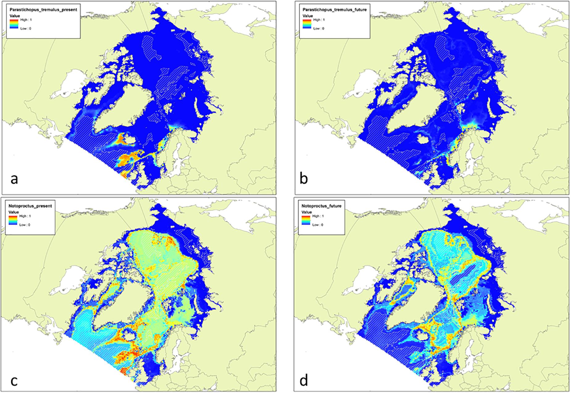
Figure 3. Habitat suitability maps for the two biggest losers [the Boreal sea cucumber Parastichopus tremulus (-53%): (A,B); and the Arcto-boreal polychete Notoproctus spp. (-36%): (C,D)] in the study area based on the results from the MaxEnt model (see Table 1). Maps show present (A,C) and predicted future (B,D) distributions for the two species. All models predict the expected probability of occurrence from 0 (0% probability; blue) to 1 (100% probability; red).
Surprisingly, both calcifiers (in general and by phylum) and Arctic (compared to Arcto-boreal or Boreal) taxa were found to be resilient to the projected environmental changes in terms of group mean response. Calcifiers were slightly more vulnerable on average than non-calcifiers (6.1 vs. 2.8% mean habitat loss) but the difference was not significant due to high intra-group variability (t-test, P = 0.18, Figure 4). Neither biogeographic affinity nor higher taxonomic level had a significant influence on the group-mean change in habitat (one-way ANOVA tests, P = 0.39 and 0.80, Figure 4). When Arcto-Boreal and Arctic taxa were combined, their mean habitat loss was less than for Boreal taxa (2.9 vs. 10.9% habitat loss, P = 0.043). Typically, heavily calcified taxa from the Mollusca and Echinodermata phyla have been suggested to suffer greatest from acidification (Hale et al., 2011). Our analysis suggested that only 24 and 25% of the taxa in these phyla, respectively, would experience range reductions, compared to 45–100% for other phyla (Supplementary Table S2). Similarly, only 12% of Arctic taxa lost habitat, compared with nearly 50% of Arcto-boreal and Boreal taxa (Supplementary Table S2). Results were the same for all analyses whether the absolute or percent change in suitable habitat was analyzed. The 3-factor main effects ANOVA also indicated no significant factor effects (biogeography: F = 2.1, df = 2, P = 0.14; calcification: F = 1.9, df = 1, P = 0.17; higher taxonomic level: F = 0.70, df = 4, P = 0.59).
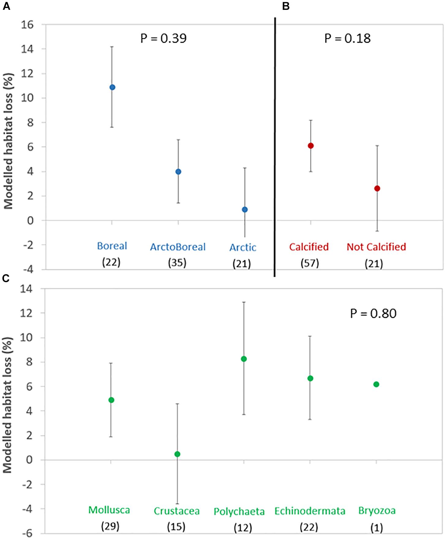
Figure 4. Mean (±1 SE) percent habitat loss for benthic taxa between the present (1978–2008) and the end of the 21st century (2090–2099). P-values of analyses of variance are included for comparisons of species grouped into: (A) biogeographic zone, (B) calcification status, and (C) higher taxonomic group. Number of taxa in each group is indicated by the number in parentheses under the group name.
The data we extracted from the OBIS database were at both the species and genus levels. In most cases, genus-level taxa were assigned to broader biogeographic zones (e.g., ArctoBoreal) because they include several species. We tested for this potential bias by analyzing only the data for taxa identified to the species-level or where it was reasonably certain that the taxa found could be ascribed to either Boreal or Arctic zones. Results of these analyses with 23 fewer taxa were nearly identical to those for the entire data set (3-factor main-effects ANOVA: biogeography: F = 2.4, df = 2, P = 0.10; calcification: F = 0.89, df = 1, P = 0.35; higher taxonomic level: F = 0.23, df = 4, P = 0.92).
Discussion
We found little evidence to support the belief that Arctic taxa are more sensitive than taxa with more southerly or cosmopolitan distributions, nor did we find that calcifiers as a group are more sensitive to projected climate-related changes than non-calcifiers. Models did indicate, however, that individual taxa can experience considerable changes in suitable habitat under future scenarios, with potentially significant ecological consequences.
Roles of Niche-Defining Parameters
When fitting MaxEnt models, temperature was the most important factor determining current suitable habitat for more than two-thirds of the taxa studied. This should come as little surprise as temperature is one of the main factors used to delineate biogeographical provinces (Longhurst, 1998), so studies over a large spatial scale with strong temperature gradients such as this are likely to show an important temperature effect. Temperature was also identified (by MaxEnt modeling) as the most important factor for mollusk and crustacean species distributions at local scales in an Arctic fjord (Drewnik et al., 2017). Temperature can act in many ways, and may be viewed as a “master parameter” that works directly through thermal tolerance for survival and/or reproduction (e.g., Wethey and Woodin, 2008), or indirectly through its impacts on, e.g., primary production, ice cover, and zooplankton and microbial grazing pressure, all of which could affect benthic food supply (Maar and Hansen, 2011). Shifts in community structure of Barents Sea benthos and fish have been noted, with the southern limit of Arctic communities moving northward during warming and retreating again southward during cooling periods (Blacker, 1965; Matishov et al., 2012; Fossheim et al., 2015). These changes were attributed to temperature, but it is unclear whether they were direct tolerance effects or something more indirect. It is important to note, however, that some high-latitude taxa have very narrow temperature ranges over which they occur, making them particularly vulnerable to climate-driven changes (Pörtner et al., 2014; Morley et al., 2019).
We used aragonite saturation state to represent the degree of potential species response to ocean acidification, but we acknowledge that this may not be the only relevant carbonate system driver. Whereas most of the calcifying taxa we studied produce aragonitic skeletons (Mollusca: Kukliński, unpublished data), there is also a large number of organisms included in our study which use calcite with varying degrees of Mg incorporation (Echinodermata, Bryozoa, Cirripedia: Kuklinski and Taylor, 2009; Iglikowska et al., 2017, 2018). In addition, some species may be more sensitive to pH or pCO2 or combinations of OA stress. However, we suspect that using only one parameter (aragonite saturation state) provides a reasonable first approximation, since most changes are expected to be quite strongly correlated between different carbonate system parameters (e.g., Figure 9 in Wallhead et al., 2017).
We included depth in our distribution models, even though it will not change significantly in the near future. Depth can often reflect a number of linked parameters important for an organism’s habitat state, such as sediment grain size, bottom currents, and vertical flux of particulate organic carbon (i.e., a proxy for food for many benthic organisms). Maintaining homeostasis under conditions of ocean acidification, for example, is thought to require more energy, and, as such, may only be possible when sufficient resources are available for affected organisms (Pansch et al., 2014). Increased metabolic rates due to higher temperatures may enhance this challenge (Pörtner, 2008). Primary production in the Barents Sea is predicted to change, both quantitatively and spatially, due to climate change (Slagstad et al., 2015). Clearly, inclusion of depth in the model will not account for all of this, but given the strong relationship between depth and vertical flux, we expect use of depth as one of the niche parameters to some extent accounted for spatial differences in food supply, in addition to partially controlling for other habitat parameters.
Accuracy of Environmental Data
The pan-Arctic SINMOD model, used here to provide bottom water temperature and aragonite saturation state, has been extensively tested and bias-corrected using field measurements (Slagstad et al., 2015; Wallhead et al., 2017). We therefore consider that the hindcast data used to define faunal niches are unlikely to have been a major source of bias. Projected changes for the 2090s are, however, subject to numerous model uncertainties and an ensemble approach would likely be required to quantify these. Nevertheless, we know that SINMOD gives bottom water projections that are comparable with global and other downscaling models, and it is sufficient for this study that the model gives plausible projections for the chosen climate change scenario (SRES A1B). For end-of-century simulations, the dominant source of uncertainty is likely to be the climate change scenario itself (Hawkins and Sutton, 2009). Water depth estimates for the pan-Arctic region are also not without uncertainty (e.g., the absolute differences between plausible measured values and the interpolated bathymetry products had median = 6 m, 95th percentile = 103 m) but it seems unlikely that such errors could significantly bias our estimates of mean habitat loss.
Surprising Robustness of Habitat Suitability
Given the reported higher vulnerability of polar organisms to ocean warming (IPCC medium confidence, Pörtner et al., 2014) and of highly calcified organisms to ocean acidification (IPCC high confidence, Ibid), the fact that our projections for benthic taxa at high northern latitudes show no clear increase in habitat loss for Arctic or calcifying species may seem surprising. It leads us to question whether something could have been lost in the complexities of the MaxEnt analysis, and if the results might be understood or corroborated by simpler analyses based on the statistics of the environment where the different species were found.
A first reason to expect higher Arctic vulnerability is that environmental changes for Arctic species may be larger under climate change, due to rapid loss of ice cover/thickness and stronger warming in polar regions (Smetacek and Nicol, 2005; Brierley and Kingsford, 2009; Doney et al., 2012). However, if we consider the median projected bottom water temperature change at the sampled presence points for each species (see Figure 5A), the species-mean warming is slightly higher for non-Arctic species (2.3 vs. 1.8°C, P = 0.04, t-test, unequal variances). Figure 5A also shows that the warming is much more consistent for Boreal species than for non-Boreal species (standard deviation = 0.15 vs. 0.87°C; P < 10–11, F-test). Regarding the median decreases in aragonite saturate state at sampled points (Figure 5B), the mean decreases are again slightly larger for non-Arctic species (0.87 vs. 0.63, P < 10–3, t-test). So at least for bottom water temperature and saturation state, it seems the environmental changes are not larger for Arctic species, as one might have anticipated from Figure 1. Furthermore, there are no significant correlations between the median environmental changes and the % habitat loss (Figures 5A,B).
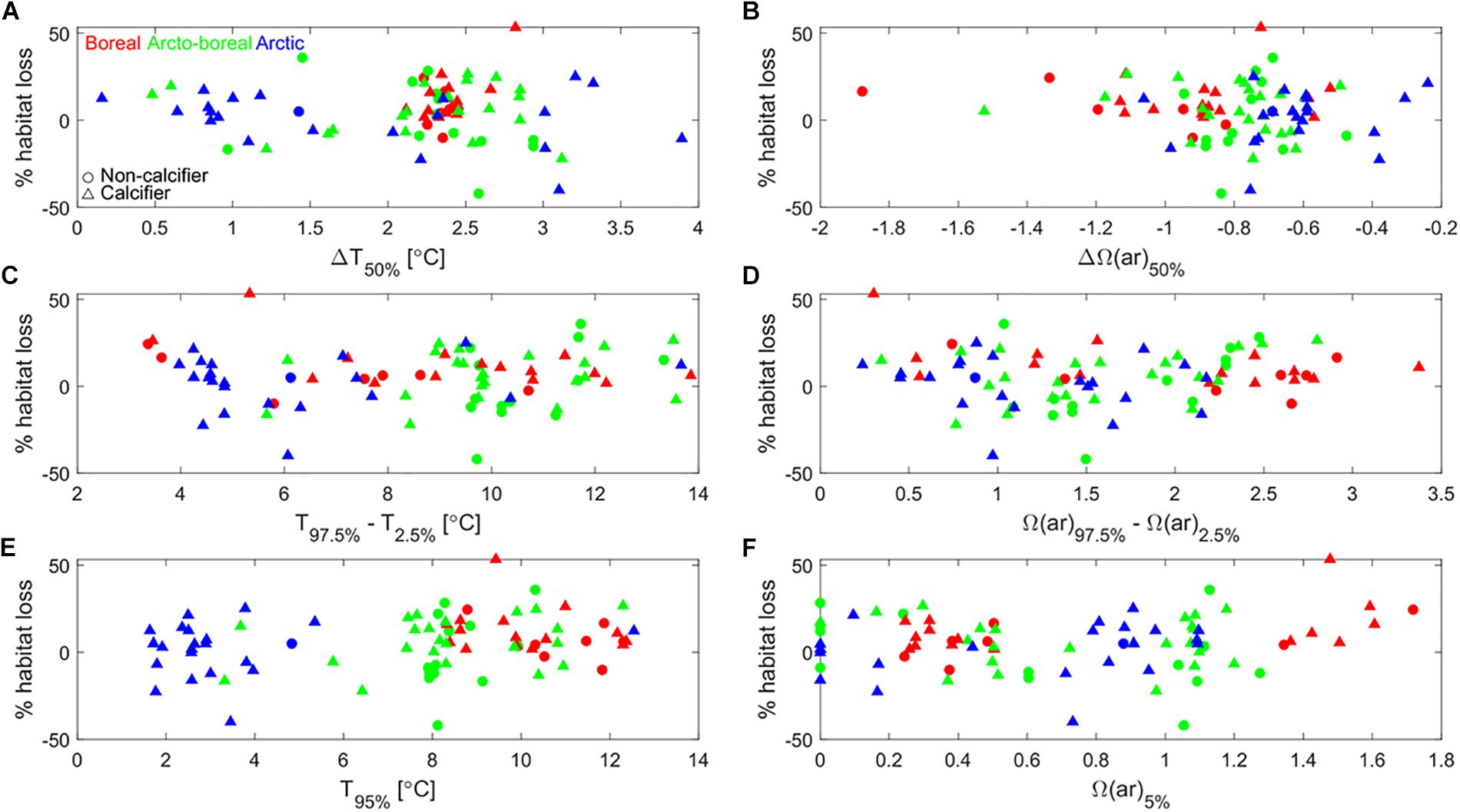
Figure 5. Environmental statistics over sampled presence locations vs. percent habitat loss from MaxEnt for Boreal (red), Arcto-boreal (green), and Arctic species (blue), and for both calcifiers (triangles) and non-calcifiers (circles). X-axes show the median projected changes in temperature (A) and aragonite saturation state (B), the 95% ranges in hindcast temperature (C) and aragonite saturation state (D), the 95th percentiles of hindcast temperature (E), and the 5th percentiles of hindcast aragonite saturation state (F). Projected changes are from the SINMOD projections (2090s vs. 1978–2008 under SRES A1B) interpolated to the presence locations; hindcast variables are from the bias-corrected SINMOD hindcast, interpolated to the presence locations and averaged over the 5 years preceding each sample date.
A second basis for high Arctic sensitivity is the idea that polar organisms have narrow environmental tolerance ranges, e.g., a “stenothermal” characteristic due to low energy-demand lifestyles and specific adaptations to cold water (Pörtner et al., 2014; Morley et al., 2019). We can test this by considering the 2.5−97.5% ranges in bottom water temperature and aragonite saturation state at the sampled presence points as tolerance metrics for each species (Figures 5C,D). Here we find that Arctic species do have somewhat narrower ranges that non-Arctic species on average (6.0 vs. 9.6°C, 1.2 vs. 1.8; P < 10–3, t-tests). However, variability in tolerance ranges is large within each group (Figures 5C,D), and there are no significant correlations between % habitat loss and tolerance ranges for temperature or saturation state (or indeed water depth, not shown). The rather moderate differences in mean tolerance range may in part reflect a higher level of historical variability in Arctic vs. Antarctic systems, at least for temperature (Pörtner et al., 2014). Arctic shelf systems have experienced, even in the past 150 years, several cycles of warming and cooling within the range we are observing today, and Arctic benthic fauna have expanded or retreated on decadal scales accordingly (e.g., Blacker, 1965).
A third basis for high Arctic sensitivity is the idea that polar organisms will have their habitat “squeezed out” under global change, either because they cannot move to higher latitudes in response to warming (Pörtner et al., 2014; Renaud et al., 2015), or because critical thresholds of saturation state will be approached first in the Arctic under ocean acidification (Feely et al., 2009; Steinacher et al., 2009; Ciais et al., 2013). If we consider the 95th percentile of bottom water temperature at the presence locations as a simple metric of upper thermal limit (Figure 5E), we find that Arctic species do indeed have a significantly lower upper thermal limit on average (3.3 vs. 9.2°C, P < 10–12, two-sample t-test). However, there is only a marginally significant correlation between % habitat loss and upper thermal limit (Pearson’s r = 0.23, P = 0.04). Considering the 5th percentile of aragonite saturation state at presence locations as a lower tolerance limit and potential predictor of vulnerability to acidification, we find no significant difference between Arctic vs. non-Arctic species, and no significant overall correlation with % habitat loss (Figure 5F).
With regard to the paradigm of higher sensitivity of calcifying species, we find no significant difference in species-mean 5th percentiles of aragonite saturation state at presence locations for calcifiers vs. non-calcifiers (0.71 vs. 0.67, P = 0.76, t-test), and both categories contain species with 5th percentiles much less than 1, and in several cases < 0.2 (Figure 5F). Such tolerance of corrosive water may be partly explained by physiological mechanisms associated with the calcification process, particularly in these often heavily calcified taxa, which are already adapted for internal control of carbonate saturation state at the site of precipitation (Hendriks et al., 2015). Considerable variability in response to ocean acidification has been shown in experimental manipulations (Kroeker et al., 2011; Vihtakari et al., 2016), and naturally high environmental variability in some habitats (shallow waters, vegetated substrate) may also help to promote tolerance via phenotypic plasticity and local adaptations (Hofmann et al., 2010). Such mechanisms may make the species less susceptible to modest decreases in saturation state, even at under-saturation levels, although food supply may mediate the ability of an organism to regulate conditions for calcification (Ramajo et al., 2016).
Analysis of Habitat Losses in Niche Space
It is worth noting that neither large environmental changes nor narrow tolerance ranges will necessarily result in high species habitat loss; if climate change produces enough new habitat, the net loss of habitat may be zero (or indeed negative) no matter how large the changes or narrow the tolerances. Rather, large changes and narrow tolerances will likely result in large (negative or positive) changes in suitable habitat area. To better understand the projections, it can be helpful to consider the calculation of % habitat loss in niche space – here a 3D space of (temperature, saturation state, water depth). The niche space can be divided into a grid of subvolumes, where the ith subvolume “contains” a physical area of habitat in the present and in the future. The MaxEnt algorithm essentially determines an occupancy probability Pji for the jth species and ith niche-space subvolume by fitting a complex preference function to the present-day niche occupancy data (Merow et al., 2013). Assuming no change over time in this niche-space preference function (ruling out e.g., genetic adaptation), the net change in habitat area Hj for species j is given by:
It follows that the projected habitat losses can in large part be explained by the changes in niche subvolume area content . These latter are entirely independent of species and the MaxEnt procedure, and depend only on the present and future environment (here based on the SINMOD biogeochemical model and the high-resolution bathymetry products).
The habitat area changes over niche space can be visualized on a 2D grid over temperature (T) and aragonite saturation state (Ω(ar)) by integrating over the water depth dimension (Figure 6A). The largest losses are in the red cells around (-2 ≤ T < 1°C, 1 ≤ Ω(ar) < 1.5), while the largest gains are in the blue cells around (−2 ≤ T < 1°C, 0 ≤ Ω(ar) < 0.2) and (0 ≤ T < 5°C, 0.4 ≤ Ω(ar) < 1). In order to be a “winner” under the projected environmental change, a species needs to have an occupancy probability or niche preference function Pji that favors the niche subvolumes that gain habitat area. This requires that its present-day sampling distribution over niche space gives evidence that the species can tolerate the winning blue cells. For example, the biggest winner, the amphipod B. gaimardii (+42% habitat area), has a widespread niche space distribution (magenta crosses). Comparing this to the sampling distribution over all species (the TGS, black dots), the MaxEnt algorithm infers a strong tolerance of low Ω(ar) and a thermal window that comfortably contains the winning range (0 ≤ T < 5°C). This allows B. gaimardii to make large area gains in the future Barents Sea, Bering Strait, Chukchi Sea, and on the East Siberian shelf between 50 and 500 m (Figures 1B,E, 2A,B). By contrast, the biggest loser, the sea cucumber P. tremulus (-53% habitat area), has a much more confined sampling distribution in niche space (magenta circles), suggesting limited tolerance of undersaturated water (Ω(ar) < 1) and a thermal window of roughly 4–10°C. Consequently, P. tremulus loses habitat in the North Atlantic and becomes increasingly confined to the Norwegian shelf shallower than 500 m (Figures 3A,B).
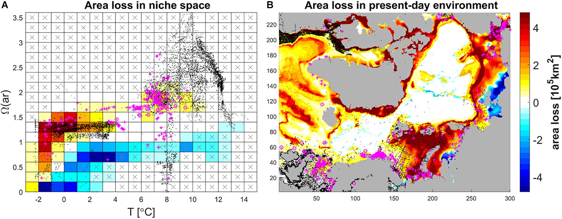
Figure 6. Niche habitat area loss in niche space (A) and mapped to the present-day environmental conditions over the SINMOD grid (B). Area losses (color scale, same in both subplots) are calculated from bias-corrected SINMOD output (2090s averages under SRES A1B vs. 1978–2008 averages from hindcast). Area losses in niche space (A) are integrated over the water depth dimension. Black dots show the sampling distributions of the OBIS presence data in niche space (A), calculated from bias-corrected SINMOD averages over 5 years preceding each sample date, and the presence locations in geographic space (B). Magenta crosses (+) show the sampling distributions of the biggest winner, the Arcto-boreal amphipod Byblis gaimardii (+42% habitat area), while magenta circles (o) show the sampling distributions of the biggest loser, the Boreal sea cucumber Parastichopus tremulus (-53% habitat area). Gray crosses (x) in (A) show cells in niche space that contain no physical area in the present-day environmental conditions (from bias-corrected SINMOD averages over 1978–2008, summing over all water depths).
Figure 6A also sounds a note of caution regarding our projections: the sampling distribution of presences (black dots) is highly non-uniform over niche space, and in particular the winning niche cells (blue colors) are strongly undersampled. For several winning cells, the present-day niche area is zero (indicated by a gray “x”); these are new niches that do not exist yet in the pan-Arctic region. Although the MaxEnt procedure is rarely strictly extrapolating with respect to the 3D convex hull (see section “Materials and Methods”) it is often being used to make bold interpolations based on limited data. This issue, plus other potential sources of bias (e.g., gear biases), reduce our confidence in the projections for individual species habitat loss, although we suspect a lesser impact of sampling bias on the significance of differences between group means. Our first attempt at running the analysis used the default MaxEnt assumption of uniform sampling effort over the pan-Arctic grid (a clearly untenable assumption, see Figure 6B); this led to much larger group-mean habitat losses (59–82%), but mean losses of Arctic species (75%) were still not significantly different to those of boreal (59%) or Arcto-boreal species (82%). The results presented in this paper account for this first assumption.
Further insights into vulnerability and sampling needs are provided by interpolating the 3D niche space area changes onto the present-day (1978–2008 average) values over the SINMOD grid (Figure 6B). Here, any species whose present-day geographical distribution is confined to areas of niche area loss (yellow/red colors) is set to be a loser under the projected changes. Hence, we can project, independently of any MaxEnt analysis, that species with environmental tolerances that confine them to e.g., the northern Barents Sea, or the East Greenland Shelf, are likely to lose habitat under climate change. Conversely, any species that tolerates present-day conditions in the Kara Sea near the Gulf of Ob, or the shallow areas (<50 m) of the eastern Laptev Sea and East Siberian Sea, is set to win. It is thus unfortunate that relatively few species presence records from these latter areas have made it into the OBIS database, and future attempts to project future species distributions would likely be well served by more sampling effort in and/or data recovery from these particular regions.
Ecological Consequences of Distributional Shifts
Approximately half the taxa were projected to experience substantial changes in suitable habitat area (>10% increase or decrease), and some of these species are characteristic or dominant on Arctic continental shelves. The polychetes Chaetozone setosa and Spiochaetopterus typicus, the bivalve Medicula ferruginosa, the barnacle Balanus balanus, and the decapods Pagurus pubescens, Hyas araneus, and Pandalus borealis are common and characteristic taxa in the open Barents Sea and adjacent fjords. S. typicus (12% increase in habitat) and B. balanus (26% loss) are key ecosystem engineers in that the physical structure they provide is important for ecosystem function. Pandalus is an important commercial shrimp in Arctic and boreal waters, and a 17% increase in habitat was predicted. If these taxa are as strongly affected as our analyses suggest, the impact on ecosystem structure and services in the Barents region could be significant over the 21st century.
Surprisingly, one of the biggest “winners” in our analyses, the Arctic bivalve Yoldiella frigida (40% habitat increase), was described as one likely to experience substantial range retraction in an analysis based solely on temperature ranges (Renaud et al., 2015). However, the Renaud et al. (2015) projection considered only the Barents Sea. The MaxEnt algorithm predicts a much more modest increase for the Barents Sea (9%), with most of the pan-Arctic habitat increase driven by gains on the Chukchi/Russian shelves and coastal waters off Canada, Greenland, and Iceland (Figure 2D). Also, Renaud et al. (2015) assumed a hard upper temperature limit of 4°C; the MaxEnt algorithm infers some tolerance of warmer temperatures (thus allowing for the slight increase in the future Barents Sea) based on the limited presence records (41) within the hindcast timeframe (1978–2008). In fact the histogram shown in Figure 5 of Renaud et al. (2015) also suggests some tolerance to warmer waters, although this latter is based on August-only SINMOD output for 2000–2009 without bias correction or matching to sample date.
One caveat of our study is the exclusive focus on bottom water environment, while many benthic organisms reproduce via planktonic larvae that live for hours to months in the pelagic zone. A recent study of an Antarctic barnacle indicated the need to consider both stages of multi-phasic species since conditions are likely to change differently in the two ocean realms (Gallego et al., 2017). Registered presence in the OBIS database, as used in our study, integrates environmental influence on multiple life-history stages/processes from fertilization, to development and dispersal, to recruitment and juvenile stages, any of which can be acted upon by ecological (including acidification) interactions in both the water column and sea floor. Another possible caveat is our use of only two physical/chemical parameters. Many other such parameters (e.g., carbon flux, bottom-water oxygen content) may define where an organism can exist, and ecological interactions cannot be expected to be unchanged as species ranges change. Kroeker et al. (2012) found ocean acidification to alter competitive hierarchies of macroalgae, and this could have consequences for associated fauna. In contrast to what has been observed for Barents Sea fish communities (Fossheim et al., 2015), benthic community change is not likely to progress via wholesale replacement of Arctic fauna with boreal fauna. Highly mobile fish are expected to move northward and southward in response to changing extent of Atlantic Waters, whereas benthic taxa have limited mobility and range changes are more likely to vary by taxa as a consequence of life-span, dispersal ability, etc. New species combinations will likely lead to novel and unpredictable species interactions, further affecting species distributions (Pecl et al., 2017). Finally, our models are based on fixed niches so that populations follow the environmental change by shifting their geographical distributions. However, populations may adapt to tolerate novel conditions through selection by evolving traits that provide tolerance in the new environment. Although it is tempting to project future distributions that take into account evolutionary responses, scientists seldom know if, or how quickly, the climate-sensitive traits of populations can evolve (Merilä and Hendry, 2014; Jezkova and Wiens, 2016).
Conclusion
Despite acknowledged issues and uncertainties with using species distribution models, especially in poorly sampled areas like the Arctic, such models are accepted as useful in providing a first approximation of how climate change will affect biodiversity (Pearson and Dawson, 2003; Wiens et al., 2009). This study is not meant to emphasize fine-scale species-specific changes, but rather to delineate expected shifts in broad patterns. The findings reported here are surprising in the context of current paradigms regarding susceptibility to climate change. In particular, we found that for benthic species under end-of-century ocean warming and acidification: (i) mean habitat losses over taxonomic groups were generally small (0–11%), (ii) Arctic benthic species were not significantly more vulnerable than boreal or Arcto-boreal species, (iii) calcifying species were not significantly more vulnerable than non-calcifiers. The lack of sensitivity of our results to such taxonomic groupings was consistent with simpler analyses based on magnitude of environmental change and observed tolerance windows, although such criteria were individually poor predictors of the habitat loss results from MaxEnt. Sampling bias in the presence data was a major issue, and in general we expect projections from benthic species distribution models for high northern latitudes to be strongly sensitive to how this is dealt with. Analysis of niche space area changes, dependent only on the environmental data, suggested that largest future habitat losses will be for taxa now inhabiting cold/oversaturated niches (−2 < T < 3°C, 1 < Ω(ar) < 1.5, e.g., the present-day northern Barents Sea and East Greenland Shelf) while the largest gains will be for those currently found in cold/undersaturated niches (−2 < T < 5°C, Ω(ar) < 1, e.g., the present-day eastern Laptev and East Siberian Seas). The latter “winning” niches were undersampled in our dataset, and we expect that further field sampling and data recovery for these niches will be especially helpful for projecting future species distributions.
There are few similar studies from high latitudes (but see Morley et al., 2019 for Antarctic waters), mainly due to limited information about species ranges and physiological tolerances, and regional models powerful enough to project environmental parameters into the future. As more data become available and models are developed, the tools we used here can be improved, and predictions refined. As in other predictive modeling approaches, MaxEnt is a process that uses data mining and probability to forecast outcomes. When doing so, the established relationships are only based on statistical dependence between environmental and distributional data, and therefore may fail to account for physiological limits and biological interactions. Development of hybrid modeling platforms that integrate species distribution models and experimental results can facilitate higher resolution distribution models for individual taxa, which can be particularly useful for economically or ecologically influential species (Kotta et al., 2019). This work is important as changes in ranges of some of these species may have substantial impacts on ecosystem services provided by benthic communities (Pecl et al., 2017).
Data Availability
The datasets generated for this study are available on request to the corresponding author. Model output data are available on Zenodo (https://zenodo.org/record/3245446).
Author Contributions
PR, MW-K, and PK developed the study idea. JK and MR performed MaxEnt modeling. RB and DS developed the SINMOD simulations. PW analyzed and bias-corrected the SINMOD output. PK was the project leader. PR led work on the manuscript. All authors contributed to the interpretation of results and editing of the manuscript.
Funding
This work was supported by the Polish-Norwegian Research Programme operated by the National Centre for Research and Development under the Norwegian Financial Mechanism 2009–2014 in the frame of Project Contract No. Pol-Nor/196260/81/2013. Additional funding was provided by the Norwegian Foreign Ministry and its Arctic 2030 program (CoArc project), the Norwegian Research Council (“Adapting Coastal Zone Management to Ocean Acidification (ACIDCOAST)”; Grant No. 255748), the FRAM – High North Research Centre for Climate and the Environment under the Ocean Acidification Flagship, and the BONUS MARES project funded by the European Union’s Seventh Framework Programme for research, technological development, and demonstration through BONUS, the Joint Baltic Sea Research and Development Programme (Art 185), and Akvaplan-niva.
Conflict of Interest Statement
The authors declare that the research was conducted in the absence of any commercial or financial relationships that could be construed as a potential conflict of interest.
Acknowledgments
The authors are grateful for technical assistance provided by Hector Andrade. Species occurrence and bias-corrected model output data used in this manuscript are openly accessible at Zenodo (https://zenodo.org/record/3245446). Further SINMOD output from the runs used in this manuscript can be found at https://doi.org/10.5281/zenodo.886077.
Supplementary Material
The Supplementary Material for this article can be found online at: https://www.frontiersin.org/articles/10.3389/fmars.2019.00538/full#supplementary-material
Footnotes
References
AMAP (2017). SNOW, Water, Ice and Permafrost in the Arctic (SWIPA) 2017. Oslo: Arctic Monitoring and Assessment Programme (AMAP).
AMAP (2018). AMAP Assessment 2018: Arctic Ocean Acidification. Tromsø: Arctic Monitoring and Assessment Programme (AMAP).
Ardyna, M., Babin, M., Gosselin, M., Devred, E., Rainville, L., and Tremblay, J. -É (2014). Recent Arctic Ocean sea ice loss triggers novel fall phytoplankton blooms. Geophys. Res. Lett. 41, 6207–6212. doi: 10.1002/2014GL061047
Bates, N. R., Orchowska, M. I., Garley, R., and Mathis, J. T. (2012). Seasonal calcium carbonate undersaturation in shelf waters of the Western Arctic Ocean; how biological processes exacerbate the impact of ocean acidification. Biogeosci. Discuss. 9, 14255–14290. doi: 10.5194/bgd-9-14255-2012
Beaugrand, G., and Kirby, R. R. (2018). How do marine pelagic species respond to climate change? Theories and observations. Ann. Rev. Mar. Sci. 10, 169–197. doi: 10.1146/annurev-marine-121916-063304
Bellerby, R., Anderson, L. G., Osborne, E., Steiner, N., Pipko, I., Chierici, M., et al. (2018). Arctic Ocean Acidification an Update. AMAP Assessment 2018: Arctic Ocean Acidification. Tromsø: Arctic Monitoring and Assessment Programme (AMAP).
Bellerby, R. G. J. (2017). Ocean Acidification without borders. Nat. Clim. Chang. 7, 241–242. doi: 10.1038/nclimate3247
Bellerby, R. G. J., Miller, L., Croot, P., Anderson, L., Azetsu-Scott, K., McDonald, R., et al. (2014). Acidification of the Arctic Ocean in Arctic Ocean Acidification Assessment. Oslo: Arctic Monitoring and Assessment Programme (AMAP).
Bellerby, R. G. J., Silyakova, A., Nondal, G., Slagstad, D., Czerny, J., De Lange, T., et al. (2012). Marine carbonate system evolution during the EPOCA Arctic pelagic ecosystem experiment in the context of simulated Arctic Ocean acidification. Biogeosci. Discuss. 9, 15541–15565. doi: 10.5194/bgd-9-15541-2012
Blacker, R. W. (1965). Recent changes in the benthos of the west spitsbergen fishing grounds. Special Pub. Int. Comm. Northw. Atl. Fish 6, 791–794.
Brierley, A. S., and Kingsford, M. J. (2009). Impacts of climate change on marine organisms and ecosystems. Curr. Biol. 19, R602–R614. doi: 10.1016/j.cub.2009.05.046
Cheung, W. W., Lam, V. W., Sarmiento, J. L., Kearney, K., Watson, R., and Pauly, D. (2009). Projecting global marine biodiversity impacts under climate change scenarios. Fish Fish. 10, 235–251. doi: 10.1111/j.1467-2979.2008.00315.x
Ciais, P., Sabine, C., Bala, G., Bopp, L., Brovkin, V., Canadell, J., et al. (2013). “Carbon and other biogeochemical cycles,” in Climate Change 2013: The physical Science Basis. Contribution of Working Group I to the Fifth Assessment Report of the Intergovernmental Panel on Climate Change, eds T. F. Stocker, D. Qin, G. K. Plattner, M. B. Tignor, S. K. Allen, J. Boschung, et al. (Cambridge, UK: Cambridge University Press), 465–570.
Collins, M., Knutti, R., Arblaster, J., Dufresne, J.-L., Fichefet, T., Friedlingstein, P., et al. (2013). “Long-term climate change: projections, commitments and irreversibility,” in Climate Change 2013: The Physical Science Basis. Contribution of Working Group I to the Fifth Assessment Report of the Intergovernmental Panel on Climate Change, eds T. F. Stocker, D. Qin, G. K. Plattner, M. B. Tignor, S. K. Allen, J. Boschung, et al. (New York, NY: Cambridge University Press).
Doney, S. C., Ruckelshaus, M., Duffy, J. E., Barry, J. P., Chan, F., English, C. A., et al. (2012). Climate change impacts on marine ecosystems. Ann. Rev. Mar. Sci. 4, 11–37.
Drewnik, A., Wȩsławski, J. M., and Włodarska-Kowalczuk, M. (2017). Benthic crustacea and mollusca distribution in arctic fjord–case study of patterns in hornsund, svalbard. Oceanologia 59, 565–575. doi: 10.1016/j.oceano.2017.01.005
Elith, J., Graham, C. H., Anderson, R. P., Dudík, M., Ferrier, S., Guisan, A., et al. (2006). Novel methods improve prediction of species’ distributions from occurrence data. Ecography 29, 129–151. doi: 10.1111/j.2006.0906-7590.04596.x
Elith, J., Phillips, S. J., Hastie, T., Dudik, M., Chee, Y. E., and Yates, C. J. (2011). A statistical explanation of MaxEnt for ecologists. Divers. Distrib. 17, 43–57. doi: 10.1111/j.1472-4642.2010.00725.x
Feely, R. A., Doney, S. C., and Cooley, S. R. (2009). Ocean acidification: present conditions and future changes in a high-CO2 world. Oceanography 22, 36–47. doi: 10.1098/rstb.2012.0442
Fielding, A. H., and Bell, J. F. (1997). A review of methods for the assessment of prediction errors in conservation presence/absence models. Environ. Conserv. 24:38e49.
Fossheim, M., Primicerio, R., Johannesen, E., Ingvaldsen, R. B., Aschan, M. M., and Dolgov, A. V. (2015). Recent warming leads to a rapid borealization of fish communities in the Arctic. Nat. Clim. Chang. 5, 673–677. doi: 10.1038/nclimate2647
Gallego, R., Dennis, T. E., Basher, Z., Lavery, S., and Sewell, M. A. (2017). On the need to consider multiphasic sensitivity of marine organisms to climate change: a case study of the Antarctic acorn barnacle. J. Biogeogr. 44, 2165–2175. doi: 10.1111/jbi.13023
Grebmeier, J. M. (2012). Shifting patterns of life in the Pacific Arctic and sub-Arctic seas. Ann. Rev. Mar. Sci. 4, 63–78. doi: 10.1146/annurev-marine-120710-100926
Hale, R., Calosi, P., McNeill, L., Mieszkowska, N., and Widdicombe, S. (2011). Predicted levels of future ocean acidification and temperature rise could alter community structure and biodiversity in marine benthic communities. Oikos 120, 661–674. doi: 10.1111/j.1600-0706.2010.19469.x
Halpern, B. S., Longo, C., Hardy, D., McLeod, K. L., Samhouri, J. F., Katona, S. K., et al. (2012). An index to assess the health and benefits of the global ocean. Nature 488, 615–620. doi: 10.1038/nature11397
Hastie, T., Tibshirani, R., and Friedman, J. (2009). The Elements of Statistical Learning. New York, NY: Springer.
Hawkins, E., and Sutton, R. (2009). The potential to narrow uncertainty in regional climate predictions. Bull. Amer. Meteorol. Soc. 90, 1095–1107.
Hendriks, I. E., Duarte, C. M., Olsen, Y. S., Steckbauer, A., Ramajo, L., Moore, T. S., et al. (2015). Biological mechanisms supporting adaptation to ocean acidification in coastal ecosystems. Est. Coast. Shelf Sci. 152, A1–A8.
Hofmann, G. E., Barry, J. P., Edmunds, P. J., Gates, R. D., Hutchins, D. A., Klinger, T., et al. (2010). The effect of ocean acidification on calcifying organisms in marine ecosystems: an organism-to-ecosystem perspective. Ann. Rev. Ecol. Evol. Syst. 41, 127–147. doi: 10.1146/annurev.ecolsys.110308.120227
Hoppe, C. J. M., Wolf, K. K. E., Schuback, N., Tortell, P. D., and Rost, B. (2018). Compensation of ocean acidification effects in Arctic phytoplankton assemblages. Nat. Clim. Chang. 8, 529–533. doi: 10.1038/s41558-018-0142-9
Iglikowska, A., Najorka, J., Voronkov, A., Chełchowski, M., and Kukliński, P. (2017). Variability in magnesium content in arctic echinoderm skeletons. Mar. Environ. Res. 129, 207–218. doi: 10.1016/j.marenvres.2017.06.002
Iglikowska, A., Ronowicz, M., Humphreys-Williams, E., and Kukliński, P. (2018). Trace element accumulation in the shell of the arctic cirriped Balanus balanus. Hydrobiology 818, 43–56. doi: 10.1007/s10750-018-3564-5
IPCC (2014). Climate Change 2014: Synthesis Report. Contribution of Working Groups I, II and III to the Fifth Assessment Report of the Intergovernmental Panel on Climate Change, eds Core Writing Team, R. K. Pachauri and L. A. Meyer, (Geneva: IPCC).
Jakobsson, M., Mayer, L., Coakley, B., Dowdeswell, J. A., Forbes, S., Fridman, B., et al. (2012). The international bathymetric chart of the Arctic Ocean (IBCAO) version 3.0. Geophys. Res. Lett. 39:L12609. doi: 10.1029/2012GL052219
Jezkova, T., and Wiens, J. J. (2016). Rates of change in climatic niches in plant and animal populations are much slower than projected climate change. Proc. R. Soc. London B 283:20162104. doi: 10.1098/rspb.2016.2104
Kotta, J., Vanhatalo, J., Jänes, H., Orav-Kotta, H., Rugiu, L., Jormalainen, V., et al. (2019). Modelling spatial distribution patterns of macroalgae and their grazers under current and future environmental conditions by integration of distribution and experimental data. Sci. Rep. 9:1821.
Kovacs, K. M., Lydersen, C., Overland, J. E., and Moore, S. E. (2011). Impacts of changing sea-ice conditions on arctic marine mammals. Mar. Biodiv. 41, 181–194. doi: 10.1007/s12526-010-0061-0
Kroeker, K. J., Micheli, F., and Gambi, M. C. (2012). Ocean acidification causes ecosystem shifts via altered competitive interactions. Nat. Clim. Chang. 3:156. doi: 10.1038/nclimate1680
Kroeker, K. J., Micheli, F., Gambi, M. C., and Martz, T. R. (2011). Divergent ecosystem responses within a benthic marine community to ocean acidification. Proc. Natl. Acad. Sci. U.S.A. 108, 14515–14520. doi: 10.1073/pnas.1107789108
Kuklinski, P., and Taylor, P. D. (2009). Mineralogy of Arctic bryozoan skeletons in a global context. Facies 55, 489–500. doi: 10.1007/s10347-009-0179-3
Maar, M., and Hansen, J. L. (2011). Increasing temperatures change pelagic trophodynamics and the balance between pelagic and benthic secondary production in a water column model of the Kattegat. J. Mar. Syst. 85, 57–70. doi: 10.1016/j.jmarsys.2010.11.006
Matishov, G., Moiseev, D., Lyubina, O., Zhichkin, A., Dzhenyuk, S., Karamushko, O., et al. (2012). Climate and cyclic hydrobiological changes of the Barents Sea from the twentieth to twenty-first centuries. Pol. Biol. 35, 1773–1790. doi: 10.1007/s00300-012-1237-9
Merilä, J., and Hendry, A. P. (2014). Climate change, adaptation, and phenotypic plasticity: the problem and the evidence. Evol. Appl. 7, 1–14. doi: 10.1111/eva.12137
Merow, C., Smith, M. J., and Silander, J. A. Jr. (2013). A practical guide to MaxEnt for modeling species’ distributions: what it does, and why inputs and settings matter. Ecography 36, 1058–1069. doi: 10.1111/j.1600-0587.2013.07872.x
Morley, S. A., Barnes, D. K., and Dunn, M. J. (2019). Predicting which species succeed in climate-forced polar seas. Front. Mar. Sci. 5:507.
Nakicenovic, N., Alcamo, J., and Davis, G. (2000). Special Report on Emissions Scenarios, Intergovernmental Panel on Climate Change. (New York, NY: Cambridge University Press), 599.
Neukermans, G., Oziel, L., and Babin, M. (2018). Increased intrusion of warming atlantic water leads to rapid expansion of temperate phytoplankton in the Arctic. Global Chang. Biol. 24, 2545–2553. doi: 10.1111/gcb.14075
Pansch, C., Schaub, I., Havenhand, J., and Wahl, M. (2014). Habitat traits and food availability determine the response of marine invertebrates to ocean acidification. Glob. Chang. Biol. 20, 765–777. doi: 10.1111/gcb.12478
Pearson, R. G., and Dawson, T. P. (2003). Predicting the impacts of climate change on the distribution of species: are bioclimate envelope models useful? Global Ecol. Biogeogr. 12, 361–371. doi: 10.1046/j.1466-822x.2003.00042.x
Pecl, G. T., Araújo, M. B., Bell, J. D., Blanchard, J., Bonebrake, T. C., Chen, I. C., et al. (2017). Biodiversity redistribution under climate change: impacts on ecosystems and human well-being. Science 355:eaai9214. doi: 10.1126/science.aai9214
Pedersen, M. W., Kokkalis, A., Bardarson, H., Bonanomi, S., Boonstra, W. J., Butler, W. E., et al. (2016). Trends in marine climate change research in the Nordic region since the first IPCC report. Clim Chang. 134, 147–161. doi: 10.1007/s10584-015-1536-6
Phillips, S., Dudík, M., Elith, J., Graham, C. H., Lehmann, A., Leathwick, J., et al. (2009). Sample selection bias and presence-only distribution models: implications for background and pseudoabsence data. Ecol. Appl. 19, 181–197. doi: 10.1890/07-2153.1
Pörtner, H. O. (2008). Ecosystem effects of ocean acidification in times of ocean warming: a physiologist’s view. Mar. Ecol. Prog. Ser. 373, 203–217. doi: 10.3354/meps07768
Pörtner, H.-O., Karl, D. M., Boyd, P. W., Cheung, W. W. L., Lluch-Cota, S. E., Nojiri, Y., et al. (2014). “Part A: global and sectoral aspects. contribution of working group II to the fifth assessment report of the intergovernmental panel on climate change ocean systems,” in Climate Change 2014: Impacts, Adaptation, and Vulnerability, eds C. B. Field, V. R. Barros, D. J. Dokken, K. J. Mach, M. D. Mastrandrea, T. E. Bilir, et al. (Cambridge: Cambridge University Press).
Pörtner, H. O., Langenbuch, M., and Michaelidis, B. (2005). Synergistic effects of temperature extremes, hypoxia, and increases in CO2 on marine animals: from earth history to global change. J. Geophys. Res. Oceans 110:C09S10.
Ramajo, L., Pérez-León, E., Hendriks, I. E., Marbà, N., Krause-Jensen, D., Sejr, M. K., et al. (2016). Food supply confers calcifiers resistance to ocean acidification. Sci. Rep. 6:19374. doi: 10.1038/srep19374
Renaud, P. E., Carroll, M. L., and Ambrose, W. G. Jr. (2007). “Effects of global warming on arctic sea-floor communities and its consequences for higher trophic levels,” in Impactos Del Calentamiento Global Sobre Los Ecosistemas Polares, ed. C. Duarte, (Bilbao: FBBVA Press).
Renaud, P. E., Daase, M., Banas, N. S., Gabrielsen, T. M., Søreide, J. E., and Varpe, Ø, et al. (2018). Pelagic food-webs in a changing arctic: a trait-based perspective suggests a mode of resilience. ICES J. Mar. Sci. 75, 1871–1881. doi: 10.1093/icesjms/fsy063
Renaud, P. E., Sejr, M. K., Bluhm, B. A., Sirenko, B. I., and Ellingsen, I. H. (2015). The future of Arctic benthos: expansion, invasion, and biodiversity. Prog. Oceanogr. 139, 244–257. doi: 10.1016/j.pocean.2015.07.007
Slagstad, D., Ellingsen, I. H., and Wassmann, P. (2011). Evaluating primary and secondary production in an Arctic Ocean void of summer sea ice: an experimental simulation approach. Prog. Oceanogr. 90, 117–131. doi: 10.1016/j.pocean.2011.02.009
Slagstad, D., Wassmann, P. F., and Ellingsen, I. (2015). Physical constrains and productivity in the future Arctic Ocean. Front. Mar. Sci. 2:85.
Smetacek, V., and Nicol, S. (2005). Polar ocean ecosystems in a changing world. Nature 437:362. doi: 10.1038/nature04161
Steinacher, M., Joos, F., Frolicher, T. L., Plattner, G., and Doney, S. (2009). Imminent ocean acidification in the Arctic projected with the NCAR global coupled carbon cycle-climate model. Biogeosci. 6, 515–533. doi: 10.5194/bg-6-515-2009
Sunday, J. M., Bates, A. E., and Dulvy, N. K. (2012). Thermal tolerance and the global redistribution of animals. Nat. Clim. Chang. 2:686. doi: 10.1038/nclimate1539
Vihtakari, M., Havenhand, J., Renaud, P. E., and Hendriks, I. E. (2016). Variable individual-and population-level responses to ocean acidification. Front. Mar. Sci. 3:51.
Wallhead, P. J., Bellerby, R. G. J., Silyakova, A., Slagstad, D., and Polukhin, A. A. (2017). Bottom water acidification and warming on the western Eurasian Arctic shelves: dynamical downscaling projections. J. Geophys. Res. 122, 8126–8144. doi: 10.1002/2017JC013231
Wassmann, P. (2015). Overarching perspectives of contemporary and future ecosystems in the Arctic Ocean. Prog. Oceanogr. 139, 1–12. doi: 10.1016/j.pocean.2015.08.004
Wethey, D. S., and Woodin, S. A. (2008). “Ecological hindcasting of biogeographic responses to climate change in the european intertidal zone,” in Challenges to Marine Ecosystems, eds J. Davenport, G. Burnell, T. Cross, M. Emmerson, R. McAllen, R. Ramsay, et al. (Dordrecht: Springer).
Keywords: benthic invertebrates, climate warming, multiple stressors, ocean acidification, species-distribution modeling
Citation: Renaud PE, Wallhead P, Kotta J, Włodarska-Kowalczuk M, Bellerby RGJ, Rätsep M, Slagstad D and Kukliński P (2019) Arctic Sensitivity? Suitable Habitat for Benthic Taxa Is Surprisingly Robust to Climate Change. Front. Mar. Sci. 6:538. doi: 10.3389/fmars.2019.00538
Received: 30 March 2019; Accepted: 15 August 2019;
Published: 03 September 2019.
Edited by:
Elizabeth Fulton, Commonwealth Scientific and Industrial Research Organisation (CSIRO), AustraliaReviewed by:
Yong Jiang, Ocean University of China, ChinaKristina Øie Kvile, University of Oslo, Norway
Copyright © 2019 Renaud, Wallhead, Kotta, Włodarska-Kowalczuk, Bellerby, Rätsep, Slagstad and Kukliński. This is an open-access article distributed under the terms of the Creative Commons Attribution License (CC BY). The use, distribution or reproduction in other forums is permitted, provided the original author(s) and the copyright owner(s) are credited and that the original publication in this journal is cited, in accordance with accepted academic practice. No use, distribution or reproduction is permitted which does not comply with these terms.
*Correspondence: Paul E. Renaud, cHJAYWt2YXBsYW4ubml2YS5ubw==