
94% of researchers rate our articles as excellent or good
Learn more about the work of our research integrity team to safeguard the quality of each article we publish.
Find out more
ORIGINAL RESEARCH article
Front. Mar. Sci. , 06 March 2019
Sec. Coastal Ocean Processes
Volume 6 - 2019 | https://doi.org/10.3389/fmars.2019.00099
This article is part of the Research Topic Spatial and Temporal Variability of Seawater Chemistry in Coastal Ecosystems in the Context of Global Change View all 13 articles
 Jean R. Brodeur1
 Baoshan Chen1
 Jianzhong Su1,2
 Yuan-Yuan Xu1
 Najid Hussain1
 K. Michael Scaboo1
 Yafeng Zhang3
 Jeremy M. Testa4
 Wei-Jun Cai1*
Few estuaries have inorganic carbon datasets with sufficient spatial and temporal coverage for identifying acidification baselines, seasonal cycles and trends. The Chesapeake Bay, though one of the most well-studied estuarine systems in the world, is no exception. To date, there have only been observational studies of inorganic carbon distribution and flux in lower bay sub-estuaries. Here, we address this knowledge gap with results from the first complete observational study of inorganic carbon along the main stem. Dissolved inorganic carbon (DIC) and total alkalinity (TA) increased from surface to bottom and north to south over the course of 2016, mainly driven by seasonal changes in river discharge, mixing, and biological carbon dioxide (CO2) removal at the surface and release in the subsurface. Upper, mid- and lower bay DIC and TA ranged from 1000–1300, 1300–1800, and 1700–1900 μmol kg-1, respectively. The pH range was large, with maximum values of 8.5 at the surface and minimums as low as 7.1 in bottom water in the upper and mid-bay. Seasonally, the upper bay was the most variable for DIC and TA, but pH was more variable in the mid-bay. Our results reveal that low pH is a continuing concern, despite reductions in nutrient inputs. There was active internal recycling of DIC and TA, with a large inorganic carbon removal in the upper bay and at salinities < 5 most months, and a large addition in the mid-salinities. In spring and summer, waters with salinities between 10 and 15 were a large source of DIC, likely due to remineralization of organic matter and dissolution of CaCO3. We estimate that the estuarine export flux of DIC and TA in 2016 was 40.3 ± 8.2 × 10⁹ mol yr-1 and 47.1 ± 8.6 × 10⁹ mol yr-1. The estuary was likely a large sink of DIC, and possibly a weak source of TA. These results support the argument that the Chesapeake Bay may be an exception to the long-standing assumption that estuaries are heterotrophic. Furthermore, they underline the importance of large estuarine systems for mitigating acidification in coastal ecosystems, since riverine chemistry is substantially modified within the estuary.
Since industrialization, the oceans have absorbed at least 25% of anthropogenic carbon dioxide release due to fossil fuel combustion and land use change (Sabine et al., 2004; Le Quéré et al., 2017). Consequently, there has been a 30% increase in surface ocean acidity, a phenomenon called “ocean acidification” (Doney et al., 2009). Although there is global evidence of ocean acidification in open ocean waters (Bates et al., 2014), pH declines in estuaries have largely been attributed to eutrophication (Abril et al., 2004; Sarma et al., 2011). Eutrophication is the process by which additional inputs of organic matter derived from allocthonous transport and nutrient-fueled phytoplankton production stimulate respiration, lowering pH and oxygen in subsurface or downstream waters (Nixon, 1995). Anthropogenic nutrient runoff in rivers has been found to exert a larger influence on estuarine carbonate chemistry than ocean acidification (Borges and Gypens, 2010). The combination of acidification and eutrophication can result in an additional pH decline in estuaries, due to changes in buffering capacity (Cai et al., 2011; Breitburg et al., 2015). However inorganic carbon data for most estuarine systems are insufficient to define spatial and seasonal heterogeneity, which is necessary for establishing baseline pH information from which trends can be evaluated. This information gap is a serious obstacle for resource management in these economically and socially valuable systems.
The Chesapeake Bay is the largest estuarine system in the United States, with a main stem stretching 300 km long and 8–48 km wide, an average depth of 8 m, and a deep trench up to 50 m (Cerco and Cole, 1993). The water column is partially mixed and microtidal, with two-layer circulation and episodic winds dominating mixing processes (Li et al., 2005). The bay is usually divided into three major sections: an oligohaline, heterotrophic upper bay, containing the estuarine turbidity maximum; a mesohaline, generally autotrophic mid-bay, containing most of the hypoxic zone (Testa and Kemp, 2014); and a polyhaline lower bay with a balanced net metabolism (Kemp et al., 1997; Cornwell et al., 1999). Historically, one of the major water quality issues for the bay has been eutrophication, caused by an increasing human population in the watershed and land clearing and fertilization for agriculture (Kemp et al., 2005). The Chesapeake is particularly susceptible to eutrophication because of its long residence time of 90–180 days for freshwater and nutrients (Kemp et al., 2005) and circulation patterns that enhance recycling of nutrients (Boesch et al., 2001), which tends to stimulate high productivity. Many processes in the Chesapeake Bay vary strongly with season: stratification and hypoxia (Testa and Kemp, 2014); primary production, respiration, and sediment metabolism (Baird and Ulanowicz, 1989; Smith and Kemp, 1995; Cowan and Boynton, 1996); freshwater flow and sedimentation rates (Baird and Ulanowicz, 1989); groundwater recharge and nitrate leaching (Boesch et al., 2001); and wind direction and mixing (Li et al., 2005). This complex natural variability and anthropogenic eutrophication are obstacles to identifying the primary drivers of spatial and temporal variability in inorganic carbon.
Despite large public investments in the restoration of the Chesapeake Bay and ample study of nutrient, oxygen, and organic carbon cycling, few investigations have analyzed the inorganic carbon dynamics of the bay, making it difficult to ascertain the magnitude of carbon cycling, ocean acidification and eutrophication influences on changes in pH. Wong (1979) found that pH decreased with depth and increased with salinity in the James River and the lower Chesapeake Bay. He also found that TA was linearly related to salinity in the surface waters of the lower bay, but that there was a complex pattern of mixing and removal within the James River estuary. Raymond et al. (2000) determined that the York River estuary in the lower bay region was heterotrophic at most times and in most places, with strong seasonal patterns. Based on an analysis of historical pH data from a long-term monitoring program, Waldbusser et al. (2013) determined that daytime average surface pH declined over a 25-year period in polyhaline waters, but not in lower salinity regions. Cai et al. (2017) explored water column inorganic carbon dynamics at a station in the upper part of the mid-bay, focusing on pH minima in the sub-oxic zone and the implications for estuarine buffering. These studies raised important questions about whether there were significant, unobserved sources and sinks of TA in the bay that could not be resolved with existing observational data. However, there has been no previous study providing complete coverage of DIC, TA and pH distributions in the Chesapeake Bay.
The objective of this study was to measure the distribution of inorganic carbon across seasons (10 months) in the full Chesapeake Bay, and to better evaluate the bay-ocean carbon flux and vulnerability to estuarine acidification. Such studies are important for the management of valuable estuarine resources, as well as improving our understanding of spatial and seasonal changes and the underlying processes at local or regional scales for global ocean acidification research.
Ten cruises were conducted in the Chesapeake Bay in 2016: four on the R/V Rachel Carson from May 4–6, June 6–10, August 8–12, and October 10–13; and six on the R/V Randall T. Kerhin from March 14–16, April 12–13, July 11–13, September 19–21, November 14–15, and December 12–14. Carson cruises, except for May, covered the main stem along the full longitudinal axis of the bay, while the Kerhin cruises took place solely in Maryland waters, with a southernmost point approximately at the latitude where the Potomac River meets the bay. Stations (Figure 1) were selected from existing Water Quality Monitoring stations designated through the collaboration between the States of Maryland and Virginia and the Chesapeake Bay Program1. We added an Atlantic Ocean site (AO1) in the mouth of the Bay at approximately 37.061°N, 75.856°W, and an additional site south of the Chesapeake Bay Bridge called Station 858 at approximately 38.962°N, 76.380°W [previously studied by Cai et al. (2017)]. The upper bay stations start with the Susquehanna River (CB 1.1) and end with CB 3.2. The Susquehanna Flats are the shallow mudflats located between stations CB 1.1 and CB 2.1. The mid-bay stations start near the Bay Bridge at 39°N with CB 3.3 through CB 5.4. The lower bay stations start in Virginia waters south of the Potomac River mouth with CB 5.5 and end with AO1 in the Atlantic Ocean.
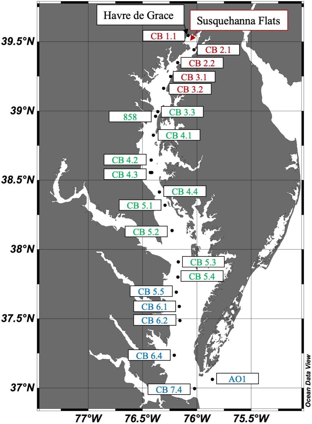
Figure 1. Map of the Chesapeake Bay with stations sampled in 2016. The Upper Bay stations labeled in red include CB 1.1 through CB 3.2.; Mid-Bay stations in green are CB 3.3 through CB 5.4; and Lower Bay stations in blue are CB 5.5 through AO1. The Susquehanna River meets the bay at CB 1.1, the Potomac River near CB 5.3, and the James River near CB 7.4.
Susquehanna River DIC and TA were sampled monthly at United States Geological Survey site #01578310 in Conowingo, MD, United States. Discharge, temperature and calcium data were obtained from the USGS water quality data portal2. For March and April, the Susquehanna River was sampled at nearby Havre de Grace, MD (39.77278°N, 76.08639°W). The Maryland Department of Natural Resources measured Secchi depth, dissolved inorganic nutrients, chlorophyll-a, and performed hydrocasts for profiles of pH, oxygen, temperature, and salinity during the R/V Kerhin cruises3.
DIC and TA samples of 250 mL and pH samples of 100 mL were collected at multiple depths via a submersible pump and filtered through a cellulose acetate cartridge filter (pore size 0.45 μm) into a borosilicate glass bottle according to previously published methods (Huang et al., 2012). During the State of Maryland monitoring cruises (March, April, July, September, November, December), hereafter referred to as “DNR cruises,” we sampled water at depths used for regular monitoring: surface, above and below the pycnocline (if present), and at the bottom. State officials determined the sampling depths by observing changes in salinity during the casts. For the May, June, August, and October cruises, subsequently referred to as “Carson cruises,” we were able to sample at a higher vertical resolution, selecting depths where salinity, oxygen, pH, or partial pressure of CO2 (pCO2) profiles showed variation, resulting in more depths sampled per station overall during those months. All DIC samples were preserved with 50 μL of saturated mercuric chloride solution (HgCl2) and refrigerated at 4°C until analysis (normally within 3–5 days). TA sample handling varied, depending on season and salinity, because HgCl2 can cause acidifying reactions in very low salinity water (S < 5) or precipitate mercury sulfide (HgS) in anoxic water, releasing acid that may affect alkalinity (Hiscock and Millero, 2006; Cai et al., 2017). For March, April, November, and December DNR cruises, DIC and TA were measured from the same samples, preserved with 50 μL of saturated HgCl2 solution and refrigerated at 4°C until analysis. During the Carson cruises, DIC and TA samples were taken in separate bottles and the TA samples were not preserved, but they were refrigerated at 4°C until analysis and analyzed at a nearby land-based lab within 24 h. During the July and September DNR cruises, all bottom water DIC and TA samples, and low salinity samples from stations CB 1.1 and CB 2.1, were taken separately, refrigerated at 4°C, and unpreserved TA samples analyzed within 72 h. pH samples were not preserved and were either measured immediately after sampling each station (Carson cruises) or refrigerated at 4°C and measured within 4–10 h of sampling (DNR cruises).
Dissolved inorganic carbon was measured by acidifying 1mL subsamples with phosphoric acid and quantifying the CO2 gas released using an infrared analyzer (AS-C3, Apollo Scitech, Newark, DE, United States). TA was measured by open cell Gran titration (Dickson, 1981) with a semi-automatic titration system (AS-ALK2, Apollo Scitech, Newark, DE, United States). Measurements were calibrated against certified reference material produced by A.G. Dickson (Scripps Institution of Oceanography, San Diego, CA, United States). Further analytical detail is described in Huang et al. (2012). pH was measured on the NBS scale at 25°C using an Orion glass electrode calibrated against three NBS standard buffers (4, 7, and 10). Confidence intervals of 95% were calculated by finding the mean percentage error for DIC and TA (unit error for pH) in duplicate samples taken during all the cruises and then adding twice the standard error, which was determined by dividing the standard deviation among the errors by the square root of the number of duplicate pairs. The resulting 95% confidence interval for the sample collection and measurements are ±0.2% for DIC, ±0.3% for TA, and ±0.017 for pH (NBS). Because the analytical precision was about ±0.1% for three repeat DIC measurements and ±0.1 to 0.2% for two repeat TA measurements, the larger uncertainties are likely caused by the inherent sampling limitations of using a submersible pump.
In order to analyze the distribution of DIC and TA in the bay, estimate the Chesapeake Bay flux of DIC and TA, and determine whether the estuary was a source or sink of inorganic carbon, we first had to calculate conservative DIC and TA values based on two endmember mixing between freshwater and seawater during estuarine transport. To do this, we plotted a line along the estuarine salinity gradient between riverine and oceanic DIC and TA values (Officer, 1979). For the Susquehanna River endmember DIC and TA values, we used monthly observational data at the Conowingo Dam (USGS Site #01578310), and in nearby Havre de Grace, MD, United States for March and April.
For the oceanic endmember, we calculated Mid-Atlantic Bight (MAB) surface layer values at 75.5°W and 36.5°N based on data from the Gulf of Mexico and East Coast Carbon cruises #1 (2007) and #2 (2012), and East Coast Ocean Acidification (ECOA) cruise (2015). Selected observations cover 17 months from 2011 to 2015. Salinity was obtained from Aquarius satellite data4 and temperature values from Optimum Interpolation Sea Surface Temperature (OISST, v2)5. MAB TA was derived from ECOA cruise data using salinity based on the linear relationship TA = (47.69(±0.99) × S) + 640.77(±31.96), r2 = 0.95, root-mean-square error = 19.6. The number of ECOA observations used was 131. For more information, studies using similar methods have recently been published, including one using the MAB data (Fassbender et al., 2017; Xu et al., 2017). MAB DIC was then calculated from seawater fugacity of CO2 (fCO2) from SOCAT (Bakker et al., 2016), the salinity-derived TA, temperature and salinity using CO2SYS (Lewis and Wallace, 1998).
We averaged the DIC, TA and salinity values for months that were sampled more than once during the 2011–2015 period. For the months of April and December, during which there was no data, we averaged the months before and after. We compared our calculated monthly MAB TA values with those previously published in order to validate the method (Signorini et al., 2013). Our values averaged just 5.2 μmol kg-1 higher (standard deviation 0.6, median 5.4). We also compared our calculated TA with the measured values at station AO1 in the bay mouth to further validate the equation, although we do not expect the two to be identical as this station is near the mouth and is likely affected by bay processes. Calculated TA values for the MAB salinity were 25.3 μmol kg-1 lower than those observed at AO1 in June, 30.0 μmol kg-1 lower in August, and 20.9 μmol kg-1 higher in October. Those differences are only 1% of the total TA value, demonstrating that the equation generates TA that is representative of the oceanic endmember and consistent over the seasonal cycle. Since the SOCAT fCO2 and TA that is very similar to previously published and observed data were used to generate the DIC, we believe it is reasonable to use these values to represent the MAB in 2016.
Previous studies have estimated riverine DIC and TA fluxes to the ocean using an effective concentration (C∗) describing what the values would be if all estuarine change was related to mixing, and the river discharge rate (Q) in the equation: Flux = Q×C∗ (Officer, 1979; Cai et al., 2004; Joesoef et al., 2017). So, to estimate the Chesapeake Bay net estuarine export flux, we first calculated a monthly linear regression of the high salinity section of the data where TA was found to be mixed linearly with the oceanic endmember (S ≥ 20 for most months, and > 15 in March and April, see Figures 7–9). Since there was no main stem cruise in January or February, we used the high salinity linear trend from December and March, respectively. Then we used the linear equation to extrapolate to zero salinity (C∗), which would represent the expected Susquehanna River value if all of the estuarine change was related to the mixing of the two end members. When multiplied by the river discharge, this value gives us the bay export. Finally, we subtracted the extrapolated river values (the effective concentration, C∗) from the measured riverine DIC and TA (C) and determined the difference related to estuarine processing. The difference was multiplied by the river discharge at the USGS station to determine the net internal accumulation, using the equation: Q × (C – C∗). Though there are significant subtidal estuarine flows of incoming and outgoing ocean water at the mouth of the bay, this method produces an estimate of the residual current because we extrapolate to zero salinity where tidal excursion is zero (residual current = river discharge, see Cai et al., 2004). However, our bay export flux could be up to 40% too low, as we did not add all other tributary discharge to the Susquehanna discharge (Q). Assuming the chemistry of other rivers are similar to the Susquehanna River, one could multiply the export flux estimated here by the ratio of the total river discharge to the Susquehanna River to derive the bay export flux. So, we also added the discharge for the Potomac and James Rivers in 2016 to the Susquehanna discharge (Q) value and estimated the full net estuarine export flux.
The most significant source of error in the net export estimation is due to the variability of the riverine DIC and TA flux, since the oceanic values were consistent and the analytical errors for the DIC and TA measurements were small. We addressed this by using a dataset of Susquehanna River sampling in 2016 that included multiple measurements per month to calculate the variation in DIC and TA. So, for the estimate of river variation, which we used as an error estimate for our export flux calculation, we used either the mean observed difference between the samples for a given month, or the mean difference for all the months, if the river was not sampled multiple times. The 2016 mean monthly variation was 97.4 μmol kg-1 for DIC and 105.3 μmol kg-1 for TA. We also tested the potential error related to the use of a high salinity trend for those months during which we did not have lower bay sampling by calculating the high salinity DIC and TA trend for June, August, and October with and without the lower bay stations and seeing the effect on the export estimate. In four of the six cases, the resultant export estimate was within the margin of error related to Susquehanna variation. However, when omitting the lower bay measurements, the calculated net DIC accumulation in June was a removal of 0.1 × 10⁹ mol C yr-1, when the one using the full bay data was an addition of 0.3 ± 0.1 × 10⁹ mol C yr-1. The October net TA accumulation without the lower bay data was an addition of 0.5 × 10⁹ mol C yr-1, when the one using the full bay data was an addition of 0.3 ± 0.1 × 10⁹ mol C yr-1. So, even though the majority of the tests showed the method to work appropriately, we have doubled the uncertainty for all of the export estimates for months in which there was no lower bay sampling. Finally, in order to explore the uncertainty in the oceanic value, we compared the effect of the difference in the calculated MAB TA and the published MAB TA on the effective concentration (C∗). Using the October data and the two estimates, we calculated C∗ as explained in the previous paragraph. The previously published DIC and TA values generated C∗ values that were 11.9 μmol kg-1, and 28.4 μmol kg-1 higher, respectively, an amount well within our uncertainty estimate for Susquehanna variability.
We investigated the surface chemical change between stations CB 1.1 and CB 2.1 in the Susquehanna Flats by calculating the impact of processes that result in DIC and TA change. First, we used the extended Redfield ratio (Redfield, 1934) (106CO2 + 16HNO3 + H3PO4 + 122H2O ↔ (CH2O)106(NH3)16(H3PO4) + 138O2 in conjunction with contemporaneous oxygen measurements to subtract the amount of DIC and TA change related to photosynthesis (assuming a photosynthetic quotient of 1, similar to that used by previous studies; Kemp et al., 1997). It was assumed that the surface waters were in equilibration with the atmosphere, and thus any change in oxygen was related to biological influence. Although this is not necessarily always the case, the stations are located close to one another and were sampled within an hour of each other, so we believe that any change in oxygen related to meteorological conditions would affect both stations. We also identified the DIC and TA change related to salinity differences between the stations by using the monthly mixing line equations to calculate the expected DIC and TA values and subtracted the mixing-related difference from the observed DIC and TA. Finally, we compared the ratio of the remaining TA to DIC change between stations to see if there was evidence of formation or dissolution of CaCO3, which would result in removal or addition at a ratio of 2:1 (Ca2+ + ↔ CaCO3 + CO2 + H2O).
Calcite saturation state values (Ω) were calculated from DIC and TA using CO2SYS version 2.1 (Lewis and Wallace, 1998). For the calculations, the following selections were made: K1 and K2 constants from Millero et al. (2006); KHSO4 from Dickson et al. (1990); NBS pH Scale; and total boron from Uppström (1974). However, the method CO2SYS uses to calculate calcite saturation results in a saturation of zero at S = 0, which underestimates the fresh water saturation state, since the riverine calcium (Ca2+) is neglected. So, we adjusted the CO2SYS calculated saturation state to account for riverine input of calcium using mean monthly [Ca2+] from USGS measurements in 2016 (see Section “Station and Cruise Information” for USGS data source). First, we determined the calcium values calculated by CO2SYS, which uses constants from Mucci (1983), concentrations from Riley and Tongudai (1967), and the equation: = (0.02128/40.087) × (S/1.80655), where S = sample salinity. Then the river value was used in the following equation to determine the corrected saturation value: ΩCorrected = ΩCO2SY S + (ΩCO2SY S × (/). For months where there were no USGS measurements (July, Sept., Nov.), we averaged the values from the month before and after. The correction is generally small: for the August data, it is an average addition of 0.25. However it is very important near the freshwater endmember.
The station map (Figure 1), as well as the salinity, DIC, TA, and pH transects in Figures 3–6 were created using Ocean Data View (Schlitzer, R., Ocean Data View, 2018)6. We used DIVA gridding with default options, including automatic scale lengths and color shading.
In 2016, the mean monthly discharge of the Susquehanna River was the lowest in a decade, only 776 m3 s-1 compared with a 60-year average of 1153 m3 s-1 (USGS data). The spring, peak freshwater discharge, or the “freshet,” was similar to previous years, but occurred in February, two months earlier than average (Figure 2). The low freshwater input resulted in high salinity and a northward shift of the estuarine turbidity maximum (ETM) (Figure 3). The center of the ETM was defined by where the salinity of the S = 1 isohaline meets the bottom (Boynton et al., 1997), and confirmed by the shoaling of light penetration. The position of the ETM affects local carbonate chemistry by inhibiting primary productivity via reduced light penetration, which can result in less DIC consumption and lower pH.
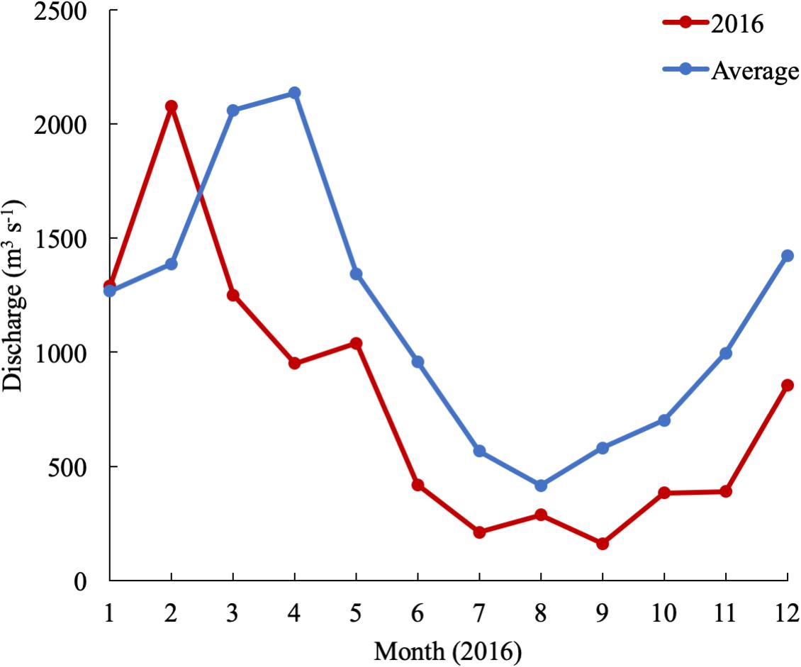
Figure 2. Susquehanna River discharge in 2016 and averaged over 60 years of data collection (USGS data).
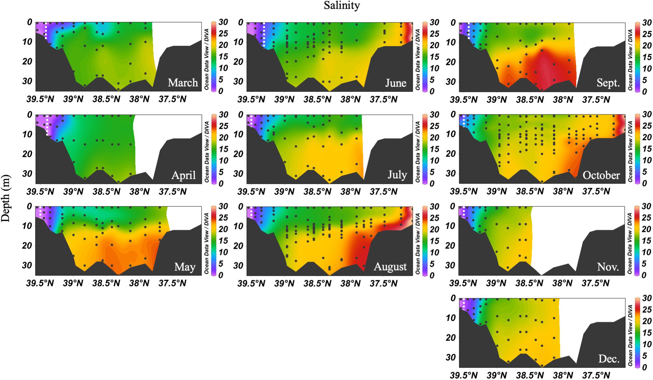
Figure 3. Depth profiles of salinity in 2016. Note that the transect lengths differ. The dividing line between the upper and mid-bay is 39°N and the mid- and lower bay is about 37.75°N. The dashed white lines are the approximate center of the ETM.
The spring carbonate chemistry in the Chesapeake Bay was strongly influenced by the arrival of the freshet and the upper bay phytoplankton bloom. At the beginning of the freshet’s influence on the bay, in March, DIC and TA increased down the bay at the surface with mixing but was largely uniform below 10 m (Figure 4). pH values in the upper bay were among the lowest all year (∼7.2), even at the surface. The ETM was centered between stations CB 2.1 and CB 2.2, except for April, when the increasing impact of the freshet pushed it downstream between CB 2.2 and CB 3.1. In April, the freshet coincided with the breakdown of the vertical gradients in salinity (Figure 3), DIC and TA (Figure 4). During May, as seasonal stratification began, DIC and TA values increased with mixing down the bay at the surface and with depth, except for some removal in the subsurface photosynthesis maximum, and were relatively uniform below the pycnocline in the mid- and lower bays. pH declined with depth and was especially low in the mid-bay in May.
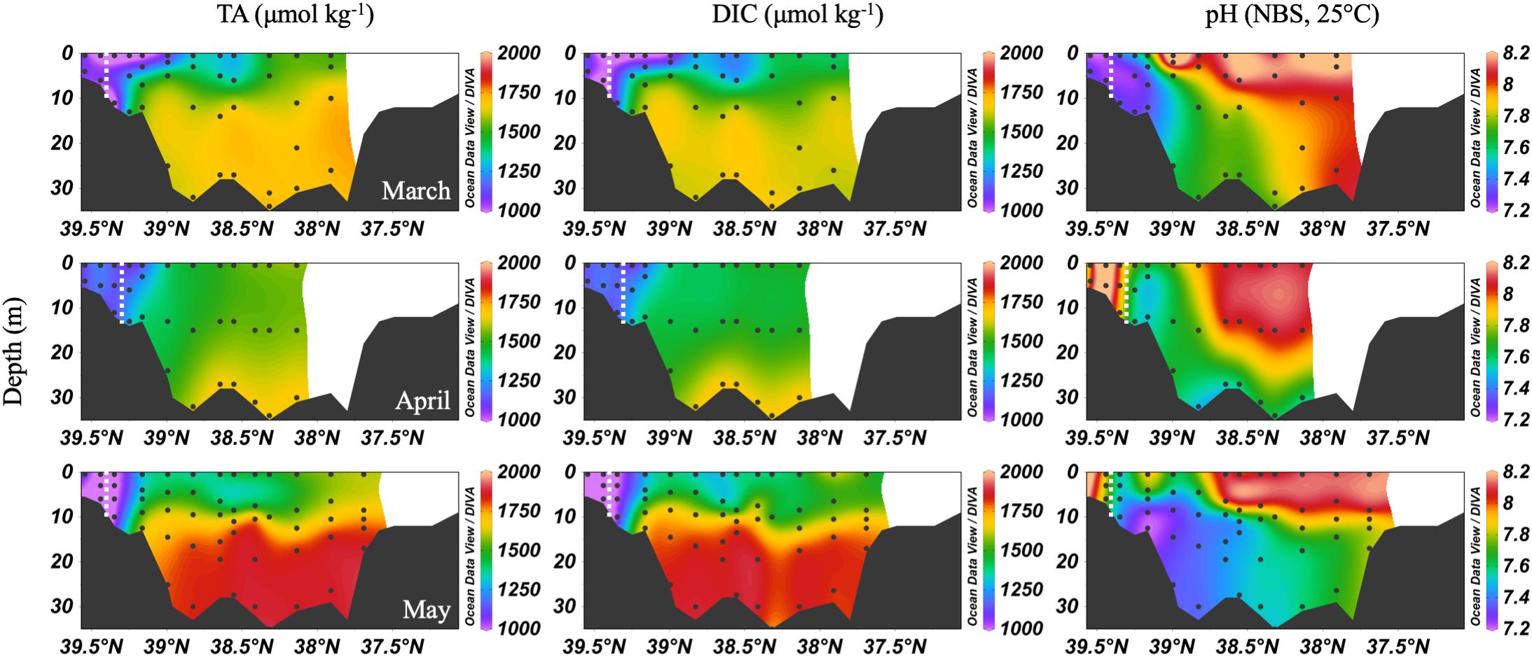
Figure 4. Depth profiles of DIC, TA, and pH in spring, 2016. Note that the transect lengths differ. The dividing line between the upper and mid-bay is 39°N. The dashed white lines are the approximate center of the ETM.
In the summer, the Chesapeake Bay was periodically hypoxic (State of Maryland Department of Natural Resources, 2016) and stratified in the main channel (Figure 5). The ETM center was between CB 2.1 and CB 2.2 in June, and between CB 1.1 and CB 2.1 in July and August, the lowest discharge months of the year. Low freshwater discharge resulted in increasing intrusion of ocean water over the season, indicated by increasing bottom water salinity, which also increased DIC and TA. In June, the DIC began to build up at depth in the mid-bay, due to the respiration of organic matter from the spring upper bay bloom. Bottom water pH decreased to a minimum value of ∼7.0 to 7.1. July had similar patterns, with a reduction of the vertical gradient at some stations due to mixing and a very shallow pycnocline. Stations CB 2.1 and CB 2.2 (the 2nd and 3rd vertical profiles in the Figure 5 plots), in the estuarine turbidity maximum, had much lower DIC and TA than CB 1.1, despite similar pH. In August, strong stratification, low freshwater input, and respiration resulted in very high and uniform DIC at depth. At the bottom in the lower bay, TA was particularly high, associated with high salinity water (Figure 3). For pH, the minimum was in the ETM and at depth in the mid-bay, due to respiration and possibly the oxidation of reduced chemical species when bottom water was mixed into the oxygenated middle depths, as previously identified during a mixing event in August (Cai et al., 2017). In August, pH at depth in the lower mid-bay and lower bay at around 38°N was high (∼7.8–8.0), reflecting the influence of the oceanic endmember and mixing with high pH surface waters at the mouth.
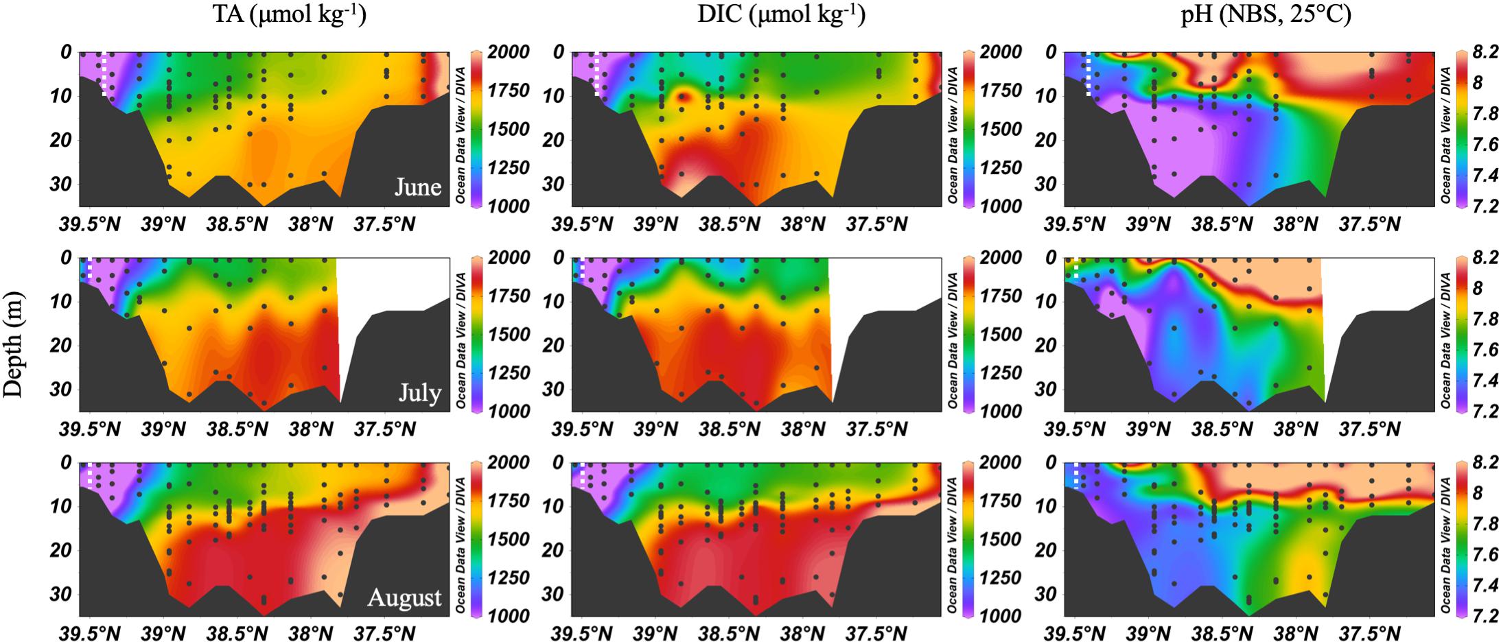
Figure 5. Depth profiles of DIC, TA and pH in summer, 2016. Note that the transect lengths differ. The dividing line between the upper and mid-bay is 39°N and the mid- and lower bay is about 37.75°N. The dashed white lines are the approximate center of the ETM.
In the early fall, water column chemistry was similar to the summer, but periodic and increasing wind-driven mixing events later reduced the vertical gradient of DIC and TA from over 300 μmol kg-1 in September to about 100 μmol kg-1 in December (Figure 6). The ETM was between CB 1.1 and CB 2.1 during the fall and winter. In September, pH was very low in the upper bay and with depth, likely a result of weakened stratification and overturn stimulating respiration and the oxidation of reduced species at depth. Later in the fall, the pH increased to the upper bay mean pH maximum (∼7.9). Notably, high productivity was evident at the surface even as late as November, with a mean mid-bay surface pH of about 8.2, the seasonal maximum value and nearly as high as the overall surface maximum of 8.3 in July. One of the highest station vertical mean pH values, 8.15, was measured in December at CB 1.1.
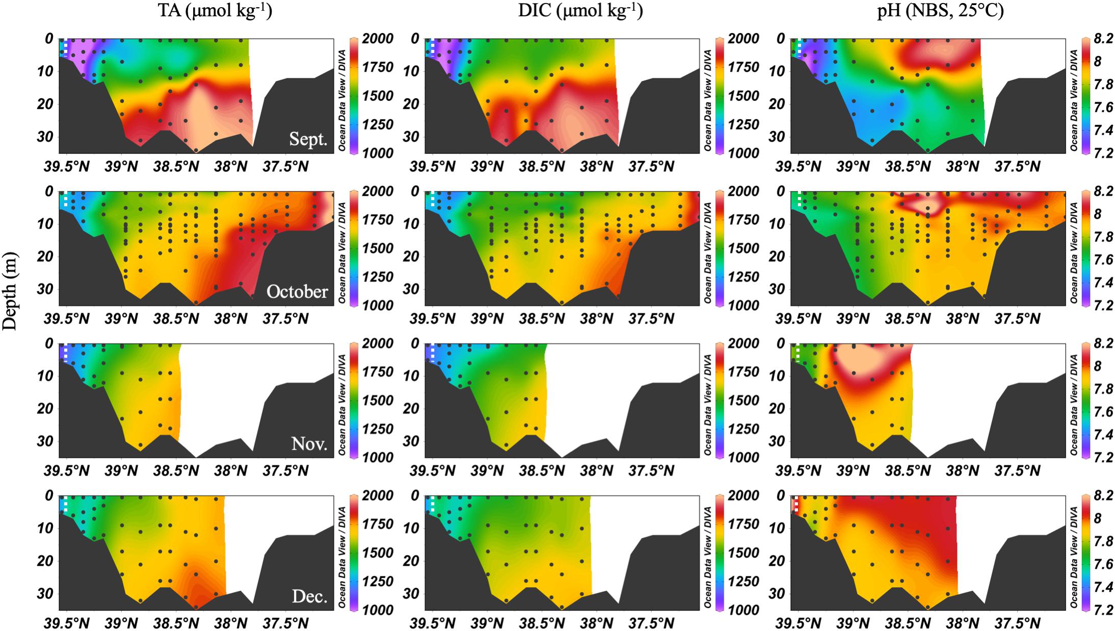
Figure 6. Depth profiles of DIC, TA and pH in fall/winter, 2016. Note that the transect lengths differ. The dividing line between the upper and mid-bay is 39°N and the mid- and lower bay is about 37.75°N. The dashed white lines are the approximate center of the ETM.
As expected, mean DIC and TA increased with salinity in the Chesapeake Bay, so they increased from the upper bay to the lower bay and with depth (Table 1). The smallest difference in DIC and TA between the upper and mid-bay average, sectional values was in the fall/winter, in December: a minimum DIC difference of 162.5 μmol kg-1 (surface) and 322.6 μmol kg-1 (bottom); and a minimum TA difference of 279.2 μmol kg-1 (surface) and 348.9 μmol kg-1 (bottom). The December pH difference was just 0.11 at the surface and 0.02 at depth. The largest difference was in the summer, in August: with a DIC difference of 447.8 μmol kg-1 (surface) and 847.5 μmol kg-1 (bottom); TA difference of 582.8 μmol kg-1 (surface) and 893.1 μmol kg-1 (bottom). The August pH difference was 0.49 at the surface and 0.21 at depth. The mid-bay and lower bay difference was also greater in summer and smaller in winter, though the DIC difference in summer was just half the TA difference, due to an enrichment of DIC in the bottom water of the mid-bay. pH increased 0.16 from the mid- to lower bay, but the difference in summer was about twice the value of the fall/winter. The saturation state of CaCO3 typically increased with salinity and decreased with depth. The upper bay was generally undersaturated, except for some stations during the productive summer and during the fall/winter. The mid-bay was typically oversaturated at the surface year-round, and undersaturated at depth during the productive and stratified months. The lower bay was supersaturated with calcite during the summer and fall/winter.
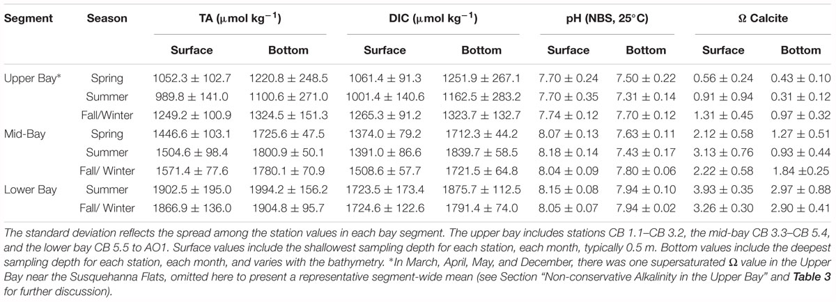
Table 1. Seasonal mean carbon parameters for bay regions in 2016.
We examined DIC and TA change along the salinity gradient by plotting a conservative mixing line between the two end members, the Susquehanna River and the Atlantic Ocean. Deviations from the line in the estuary indicate non-conservative behavior, with curvature below representing removal and above representing addition of the chemical species (Officer, 1979). Although the utility of the two-member model could be compromised if there were a third tributary, there is no other substantial freshwater source in the upper bay. Previous work has also found that many biogeochemical constituents are highly non-conservative in the Chesapeake Bay (Fisher et al., 1988).
In the spring (Figure 7), removal of DIC and TA was most significant at low salinity (S < 5), where the spring bloom begins (Malone et al., 1996), while DIC and TA changes were near conservative at middle (5 < S < 15) and higher salinities (S > 15). DIC was strongly influenced by biological activity, particularly through uptake at the surface, which was most dramatic in March, and enrichment via respiration in the bottom waters, most clearly seen beginning in May and continuing into the summer. Though the TA change with salinity was generally conservative in the spring, there was a large removal of alkalinity between CB 1.1 and CB 2.1, in an area called the Susquehanna Flats (approximately S = 0-2), that essentially resets the mixing line for the rest of the bay to Station CB 2.1 (see Section “Non-conservative Alkalinity in the Upper Bay” for more discussion). This region also often contained the ETM center, which may also contribute to TA removal. The exception was in April, when the freshet waters reached the bay with large inputs of riverine organic matter and sediments and diluted removal and addition signals (Schubel, 1968).
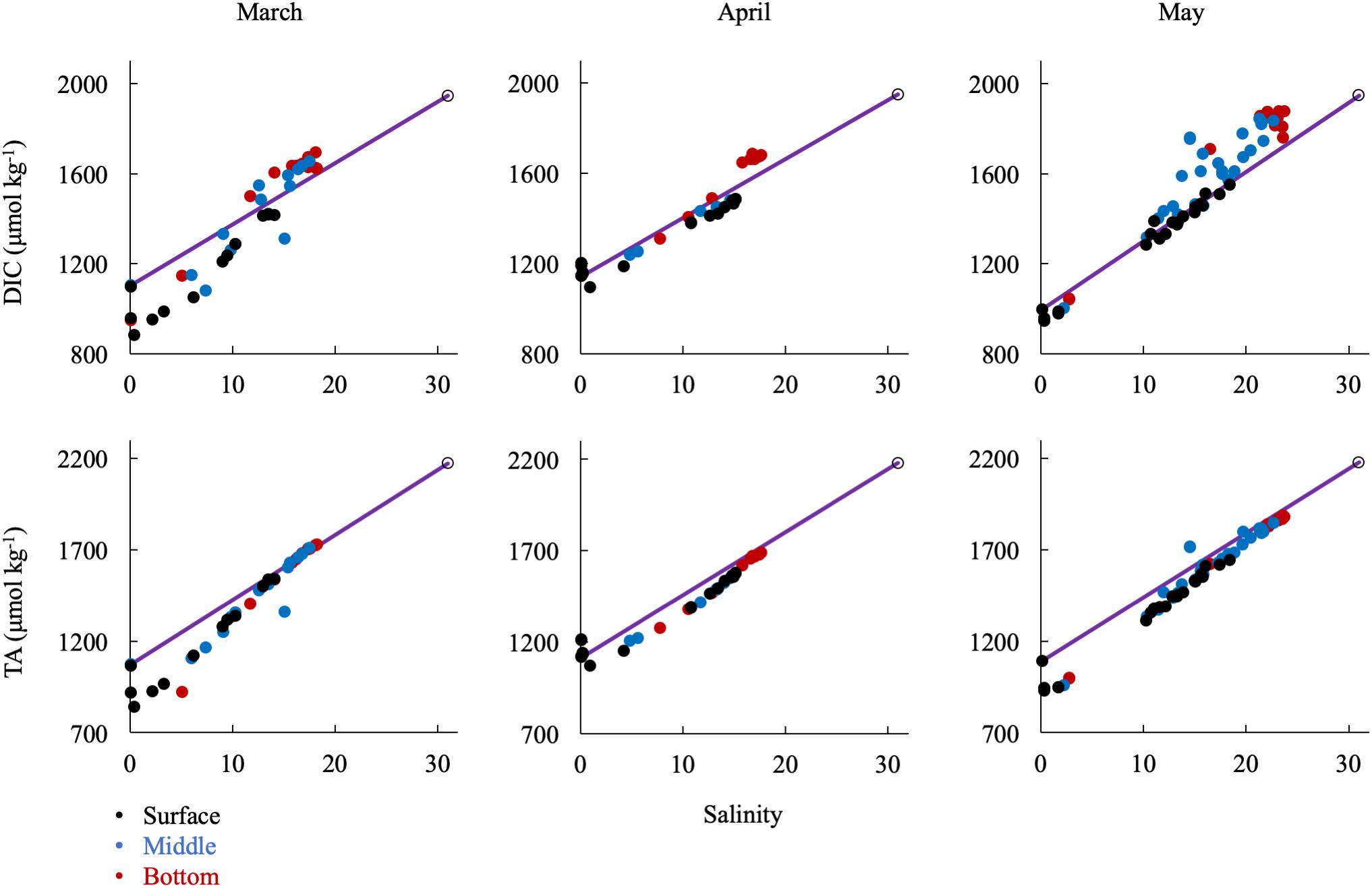
Figure 7. Relationship of DIC and TA observations in the spring to the conservative mixing line. Black dots are surface water (shallowest samples, typically < 1 m), blue are mid-column, and red are bottom water (bottom samples, dependent on bathymetry). The open circle is the approx. bay mouth value at S = 31, derived from the mixing line equation. The 95% confidence intervals are smaller than the symbol.
In the summer, when river discharge was lowest, ΔDIC and ΔTA from the conservative mixing line were very large, reflecting strong biological control on inorganic carbon (Figure 8). DIC was removed at low salinities and in the surface water and added in large amounts in the mid-salinities, reflecting the respiration signal in the sub-oxic boundary and at the bottom. TA was first removed in the low salinities via calcium carbonate (CaCO3) formation and then added in the mid- and high salinities via CaCO3 dissolution. The large addition of alkalinity via calcium carbonate dissolution in the respiration-dominated, higher-salinity waters below the pycnocline and in the mid- and lower bays is more apparent if the mixing line is drawn from station 2.1 (dotted lines in Figure 8). Over the year, conservative mixing related to salinity typically began at CB 2.1 instead of 1.1, due to the large chemical change across the Susquehanna Flats. Consequently, if the wrong freshwater endmember is used during the productive summer, TA could appear to be conservatively mixed in the mid- and high salinities, when it is in fact recycled.
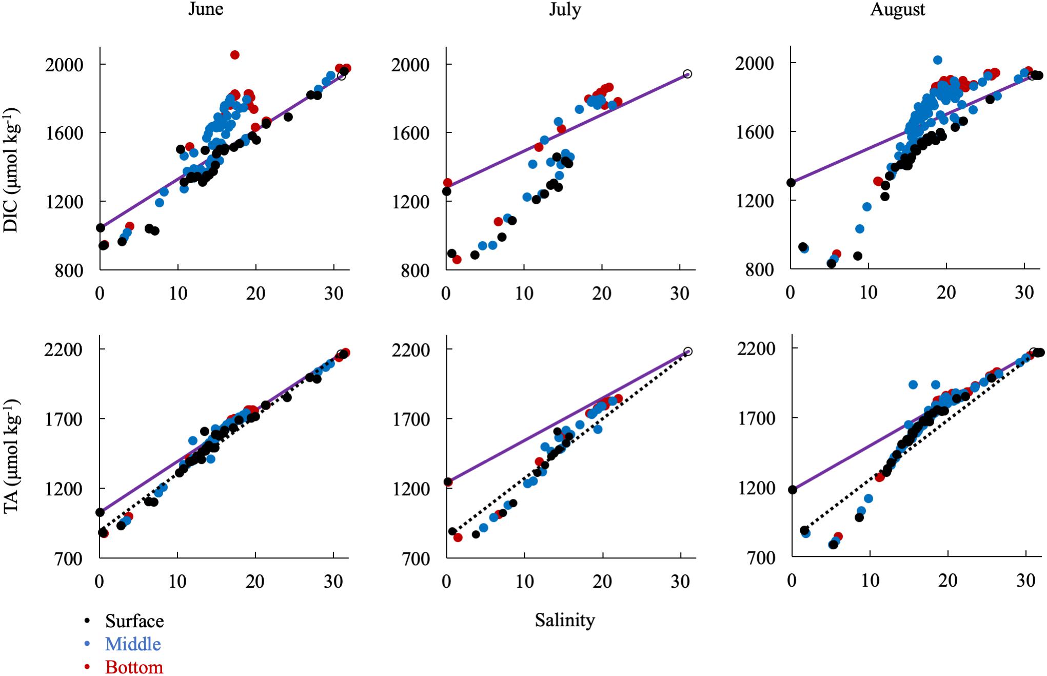
Figure 8. Relationship of DIC and TA observations in the summer to the conservative mixing line. Black dots are surface water (shallowest samples, typically < 1 m), blue are mid-column, and red are bottom water (bottom samples, dependent on bathymetry). The open circle is the approx. bay mouth value at S = 31, derived from the mixing line equation. The 95% confidence intervals are smaller than the symbol. The dotted lines show mixing from CB 2.1 to the oceanic end member.
Large removals or additions of alkalinity continued into the early fall with the breakdown of stratification (Figure 9). September had a similar DIC and TA pattern as the summer months. In October, there was a general addition of DIC and TA with increasing salinity south of the upper bay removal. Notably, there was a large alkalinity addition at mid-salinities and in the mid-bay in September and October that correlates with evidence of a small bloom (increase in oxygen and pH and decrease in DIC). Then, in November and December, the upper bay removal was absent. In fact, there appeared to be a source near the Susquehanna Flats in December, possibly due to CaCO3 dissolution after the end of summer submerged aquatic vegetation (SAV) production in the upper bay. This is especially interesting since there was consistent inorganic carbon removal during the other 8 months studied. Both months showed a non-linear, concave mixing curve that seems to describe removal of DIC and TA in the mid-salinities. The similarities of the DIC and TA curves and the fact that surface, middle, and bottom water are all on the same line eliminate several potential processes such as CO2 degassing or biological production, which would reduce DIC but not TA, and sulfide oxidation, which would reduce TA, but not DIC. It is possible that the Susquehanna River values suddenly increased before sampling or additional freshwater was mixed in the mid-bay, via precipitation and groundwater or other tributaries.
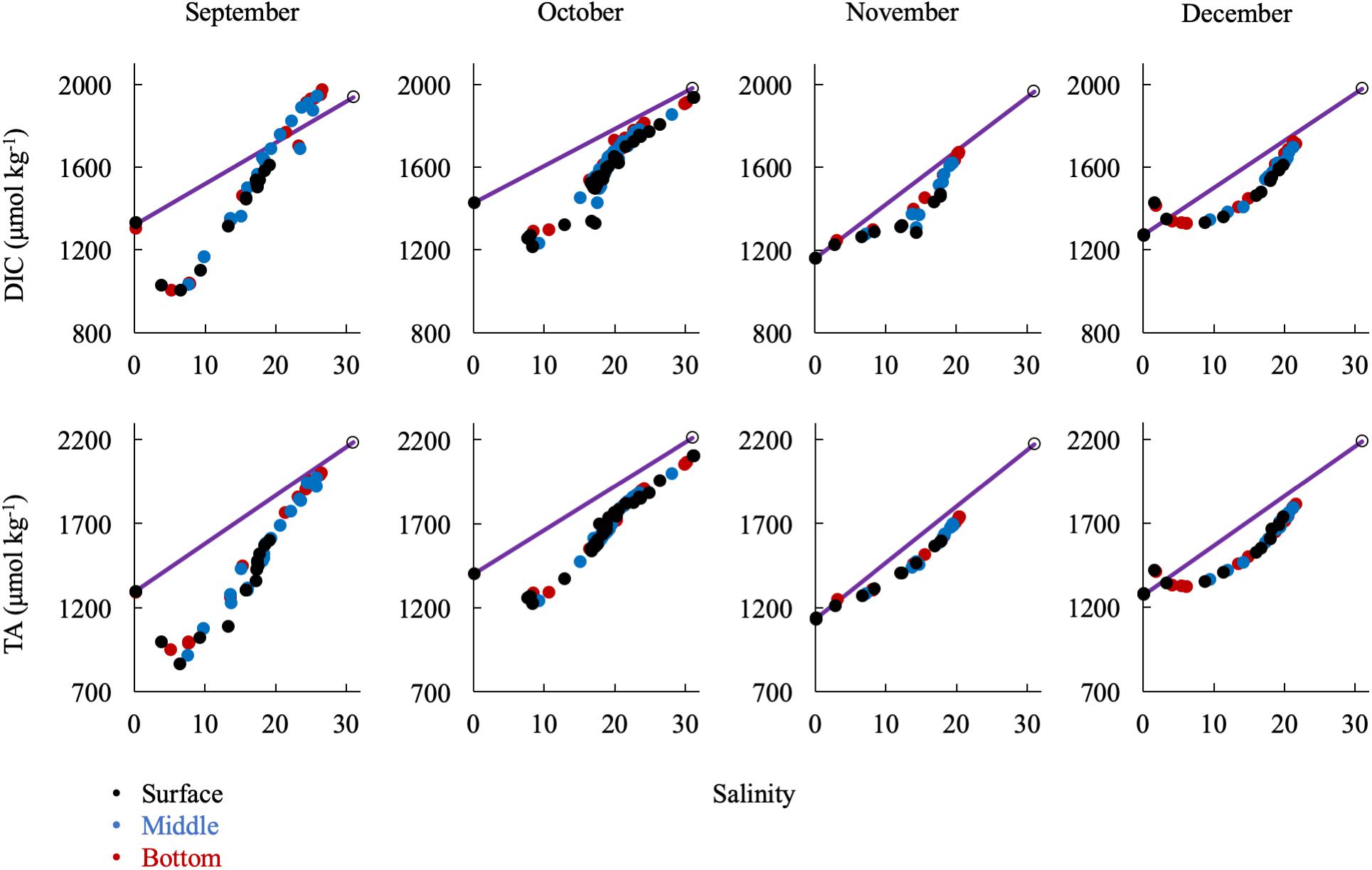
Figure 9. Relationship of DIC and TA observations in the fall/winter to the conservative mixing line. Black dots are surface water (shallowest samples, typically < 1 m), blue are mid-column, and red are bottom water (bottom samples, dependent on bathymetry). The open circle is the approx. bay mouth value at S = 31, derived from the mixing line equation. The 95% confidence intervals are smaller than the symbol.
As with other biogeochemical constituents in the Chesapeake Bay, the net estuarine export flux of DIC is positively correlated to Susquehanna River discharge, which is highest in winter and spring (Table 2). We calculated riverine DIC and TA flux using USGS monthly mean discharge data (Q) and monthly measurements of DIC and TA (C) in the following equation: Flux = Q∗C. The estimated Susquehanna River DIC and TA flux in 2016 was 27.5 ± 2.7 × 10⁹ and 26.9 ± 2.6 × 10⁹ mol C yr-1, respectively. The maximum river flux was in February, during the freshet, and the minimum in September, the month with the lowest discharge. We used the Susquehanna River to represent all riverine input, because it is the most significant tributary of the Chesapeake Bay, representing over 60% of the total freshwater input, though the Potomac (19%) and James (13%) are other large tributaries (Zhang et al., 2015). So, our riverine flux estimate represents a minimum, potentially resulting in an underestimation of estuarine removal. The James River has been found to have little impact on lower bay chemistry (Wong, 1979; Fisher et al., 1988), so it is reasonable to assume a negligible contribution of DIC and TA. While the Potomac River has higher discharge than the James, previous studies have found that its chemistry differs from the Susquehanna only on the order of seasonal variation in the Susquehanna River (Fisher et al., 1988), and that it has little impact on the main stem, since most of the river constituents are processed in the sub-estuary (Boynton et al., 1995). The Susquehanna values should not be significantly different from the Potomac River, since their values and biogeochemical processes are likely similar. So, only the difference in concentrations between the two rivers would matter in the C∗ and net internal accumulation calculations, and that difference would likely be a small amount, potentially within the uncertainty estimate we use to account for Susquehanna River variation. If we scale up the discharge to account for the all three rivers, the riverine DIC and TA fluxes are 46.0 ± 4.4 × 10⁹ and 44.7 ± 4.6 × 10⁹ mol C yr-1.
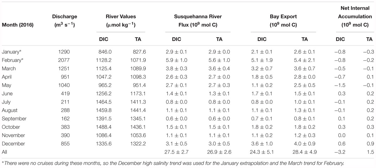
Table 2. Estimated Susquehanna River inorganic carbon flux, Chesapeake Bay net export to the coastal ocean, and net internal accumulation in 2016.
Next, we used Susquehanna River and Mid-Atlantic Bight DIC and TA values to estimate the net estuarine export flux and found that the Chesapeake Bay was a sink of inorganic carbon in 2016 (Table 2). At high salinities in the lower bay, near the ocean endmember, DIC and TA are generally mixed conservatively with salinity. So, we used a linear regression of the high salinity measurements for each month (S > 20, except for March and April, when we used > 15) to extrapolate to zero salinity, representing what the river values would be if the change along the bay was solely due to mixing of the endmembers. We multiplied the extrapolated river value (C∗) by the river discharge (Q) to determine the estuarine export flux as in the following equation:Flux = Q × C∗. Note that by this approach, we extrapolated to zero the integrated biological non-linear addition or removal during the entire estuarine mixing process. This extrapolation allows us to use the river discharge and avoid the necessity of knowing the residual water flux at the bay mouth (Officer, 1979; Cai and Wang, 1998; Cai et al., 2004; Joesoef et al., 2017). Then, the difference between the extrapolated and measured river values represent either estuarine addition, if positive, or removal, if negative. However, such internal addition or removal is also subject to subsequent modification by air-water gas exchange.
The estimated net export of DIC and TA in 2016 was 24.3 ± 5.1 × 10⁹ mol C yr-1 and 28.4 ± 4.9 × 10⁹ mol C yr-1. The annual estuarine DIC removal was -3.2 ± 5.1 × 10⁹ mol C yr-1 and TA addition was 1.5 ± 4.9 × 10⁹ mol C yr-1, making the Chesapeake Bay a sink of riverine DIC and a potential weak source of TA to the coastal ocean. However, the above net estuarine export is based on the Susquehanna discharge alone. If we scale up the numbers to account for the additional tributary discharge in order to see more realistic total DIC and TA export numbers, the net estuarine export flux is 40.3 ± 8.2 × 10⁹ and 47.1 ± 8.6 × 10⁹ mol C yr-1, meaning there was a DIC removal of -5.7 ± 8.2 × 10⁹ mol C yr-1, and a TA addition of 2.4 ± 8.2 × 10⁹ mol C yr-1. The monthly bay net export flux and the net internal production were also highly variable, related to temperature differences in atmospheric exchange and biological activity. In the late winter, spring and summer, the bay was typically a sink of inorganic carbon, though it may have been a weak source in June. A previous study found a reduction of net productivity in June and related it to higher relative respiration due to a lag between the fading spring bloom and the build-up of summer phytoplankton assemblages (Kemp et al., 1997), which would explain this result. Maximum DIC removal was in May, during the spring bloom, while maximum DIC addition was in December, when the water was colder, enhancing atmospheric CO2 invasion and reducing biological activity. Maximum TA addition was also in December, but maximum removal was in January. This seems to be a contradiction since both are during the winter season. However, January had nearly twice the freshwater discharge of December. Unfortunately, we do not have cruise data for January to compare to December, and we used the December high salinity trend for the January flux estimate. Greater resolution of the January and February conditions bay-wide would be needed to resolve the apparent conflict.
Finally, we generated an estimated carbon budget for the Chesapeake Bay (Figure 10), using published net ecosystem metabolism (NEM) (Smith and Kemp, 1995; Kemp et al., 1997) and atmospheric flux estimates (Shen et al., 2019). Notably, these studies found the bay to be net autotrophic and an atmospheric CO2 sink (12.0 × 10⁹ mol CO2 yr-1), consistent with our findings on inorganic carbon flux. We calculated a range of biological DIC removal using the lower end and average estimates of the NEM range, 33 and 50 g C m-2 yr-1, and a total bay area of 5514 × 106 m2. The resulting biological DIC removal would be -15.2 to -23.0 × 10⁹ mol DIC yr-1. Using our riverine flux estimate, the total CO2 flux from riverine and atmospheric sources was 58.0 × 10⁹ mol DIC yr-1, and when the export is subtracted, the remaining amount is -17.7 × 10⁹ mol DIC yr-1, which falls within the published NEM range. We did not explicitly estimate benthic inorganic carbon flux in our budget, though its impact on the water column was addressed via our mass-balance method, and the NEM estimate included benthic metabolism. So, if the NEM was higher than the lower-end estimate that balances our budget, potential sources of additional CO2 could include benthic respiration, groundwater or any difference between the Susquehanna River DIC and TA values used in the estimate and the concentrations in the smaller tributaries.
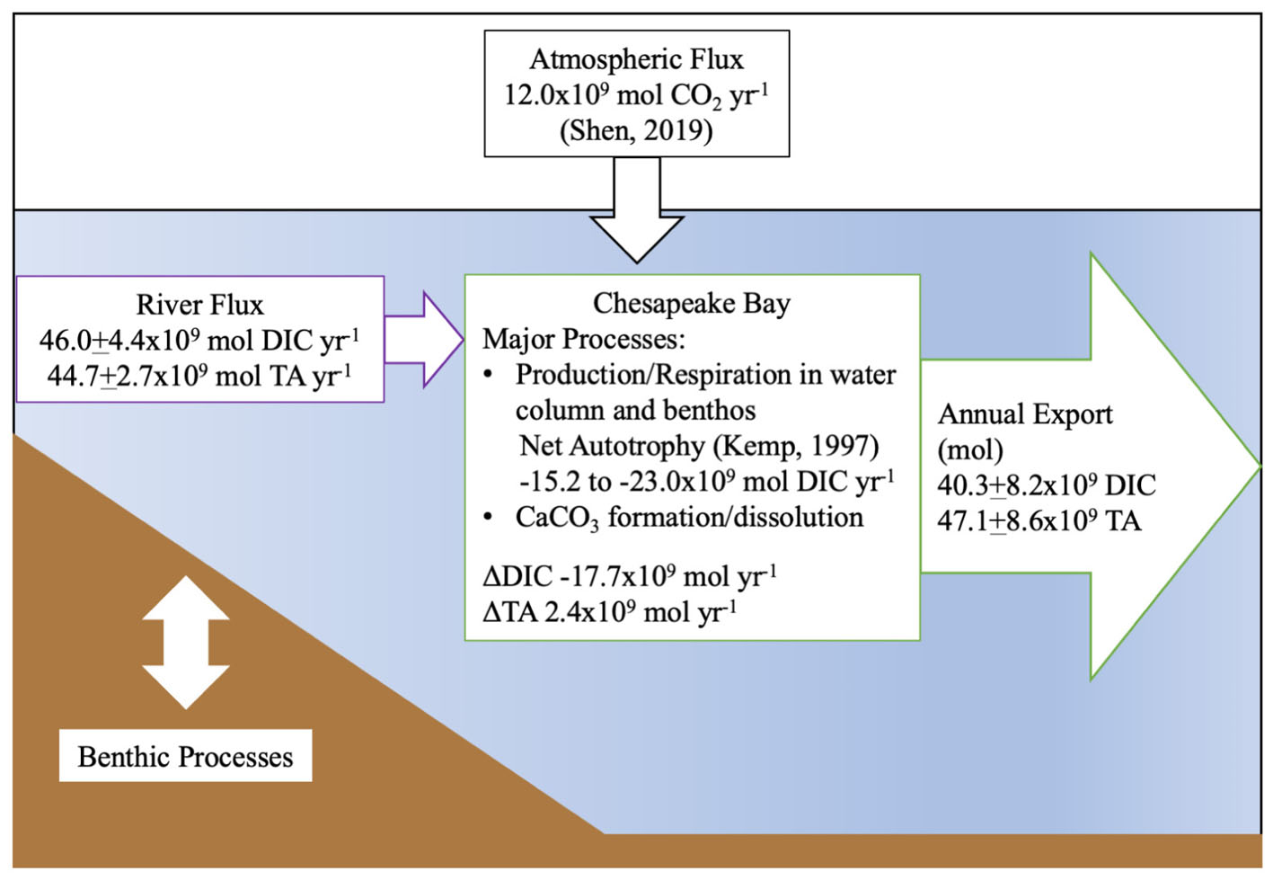
Figure 10. Summary of estimated riverine DIC and TA flux into the Chesapeake Bay and estuarine export to the Atlantic Ocean in 2016. The atmospheric flux estimate is from Shen et al. (2019) and the metabolic rate estimate from Kemp et al. (1997).
The mixing plots showed substantial and persistent inorganic carbon removal in the upper bay between stations CB 1.1 and CB 2.1. This area has experienced a large increase in SAV, shown to substantially modify local chemistry by removing total nitrogen, raising pH and improving water clarity (Gurbisz and Kemp, 2014; Orth et al., 2017). To investigate this further, we separated out the various processes that could have contributed during the months when both stations were sampled (Table 3). First, we used oxygen data from Maryland Department of Natural Resources monitoring cruises and Redfield stoichiometry to determine the apparent photosynthetic/respiratory contribution to the change in DIC and TA between the stations. We assumed that all oxygen changes were related to biological activity and not meteorological forcing, since the stations are located near one another and were sampled within an hour of each other. Then, we used the conservative mixing lines to calculate the ΔDIC and ΔTA related to increased salinity at CB 2.1. Finally, we examined the TA:DIC ratio of the remaining change between stations because when CaCO3 is formed or dissolved, the ratio of the change in TA to DIC is 2:1.
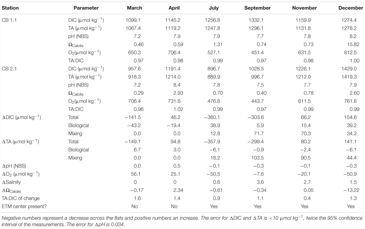
Table 3. Change in surface water chemistry across the Susquehanna Flats between CB 1.1 and CB 2.1.
During the spring bloom and freshet, the TA: DIC ratio was high. In March, oxygen increased and DIC and TA decreased by 141.5 and 149.1 μmol kg-1, likely due to photosynthesis. Yet, pH was unchanged and calcite saturation declined, though it was still undersaturated. In April, oxygen also increased between stations, however TA and DIC were added (46.2 and 94.8 μmol kg-1, respectively). There was also a fivefold increase in carbonate saturation from undersaturated to supersaturated and pH that could support the hypothesis of CaCO3 formation in the flats. The carbonate saturation returns to the CB 1.1 value at station CB 2.2, further evidence that the change is related to a process in the flats that may impact chemistry at a later time or in a difference place, as with the transport of carbonate minerals. During this month, the center of the ETM was further south, between CB 2.2 and CB 3.1, so it was not affecting the values. During the other months, the change in DIC and TA was near a TA:DIC ratio of 1, and the presence of the ETM generally resulted in expected declines in oxygen, saturation and pH, as well as addition of DIC and TA. However, November had a very low ratio, potentially related to coupled denitrification and nitrification, which are at maximum rates during the fall (McCarthy et al., 1984; Kemp et al., 1990; Lee et al., 2015; Testa et al., 2018) and is positively correlated with suspended particles as in the ETM (Damashek et al., 2016). Given the non-conservative behavior of inorganic carbon in this region, and minimal buffering resulting in relatively large changes in conditions with changes in the carbonate parameters, higher resolution study is needed, particularly given the lack of measurements within the flats area, the potential for nitrogen-related effects on alkalinity, and the analytical complications associated with the periodic presence of the ETM.
This study describes the seasonal main stem inorganic carbon distribution in the Chesapeake Bay for the first time. Generally, DIC and TA increased from surface to bottom and north to south, bay-wide, and pH decreased from surface to bottom and increased from north to south. The pattern reflects the two-layer, density-driven circulation and seasonal stratification (Li et al., 2005). Surface DIC and TA varied most over the study period because of variance in the freshwater flow, and thus salinity, though wind-driven mixing and biological activity caused seasonal changes in values. Below 15 m, average DIC and TA values were spatially consistent in the deepest parts of the main stem all year. At the surface, CO2 was removed for biological production, and then it was released in the bottom water with respiration, causing CaCO3 dissolution. This means that inorganic carbon was usually non-conservative in the bay due to biological uptake, similar to other biogeochemical constituents (Fisher et al., 1988). In terms of annual variation, the upper bay was the most variable for DIC and TA, but pH was more variable in the mid-bay. Spring was characterized by the arrival of the freshet and the beginning of the phytoplankton bloom in the upper bay. Despite large removals of DIC and TA, pH remained very low, likely related to low buffering capacity and the respiration of riverine organic material and estuarine phytoplankton. Stratification began in May, lowering pH in the mid-bay and at depth. In the summer, low discharge and stratification caused a build-up of DIC at depth and low pH, though productivity was high at the surface. In early fall, the break-down of stratification reduced the vertical gradient of DIC and TA and lowered pH, likely as reduced chemical species from the bottom were oxidized and respiration stimulated by an injection of organic material and nutrients (Lee et al., 2015; Cai et al., 2017). This detailed seasonal and spatial analysis helps to establish a baseline that can be used in the future to identify any changes in pH from eutrophication or ocean acidification.
Strong modification of the riverine flux of inorganic carbon occurred in the portion of the upper bay in which the Susquehanna Flats SAV bed is found, while downstream of CB 2.1 there was a clear pattern of linear mixing of TA over the estuarine salinity gradient. Non-conservative behavior of alkalinity in the early stages of estuarine mixing has previously been attributed to dissolution of CaCO3 causing TA addition (Abril et al., 2003, 2004). It has also been established that the organic alkalinity contribution is controlled by pH in the early stages of mixing and then becomes conservative with respect to salinity change (Cai and Wang, 1998). April measurements suggest CaCO3 precipitation and downstream dissolution, because of the high TA to DIC removal ratio and large pH and calcite saturation state increase over the flats area. However, an inorganic carbon study in the Flats is needed to resolve the issue, as well as greater resolution of the organic alkalinity contribution. Non-conservative behavior of TA in the fall and winter is likely due to a different process. Unfortunately, we have limited winter data to establish a robust high salinity trend and consequently more reliable export estimates during the fall and winter, an important time interval when TA addition was highest as percentage of river input. During the winter months, the data at all depths are in an odd concave curve, suggesting removal due to either a physical process or one affecting the full water column via vertical mixing, like sedimentary flux. The timing is coincident with maximum nitrification and denitrification rates (Kemp et al., 1990; Lee et al., 2015), so it is possible the DIC and TA addition in the low salinities and uptake in the mid-salinities during this time is in part related to nitrogen cycling. The ETM was also in the low salinity Susquehanna Flats area during the fall, which may further enhance nitrification (Damashek et al., 2016). Then, the removal with increasing salinity would be related to competing processes of photosynthesis and denitrification. Mid-bay surface removal of DIC and increased pH support the idea of an increase in productivity stimulated by nitrate addition. Another potential explanation of the alkalinity removal could be buried ferrous sulfide (FeS) oxidizing and releasing acid to the water column as low river discharge is correlated with an increase in lower bay sulfate reduction rates (Marvin-DiPasquale et al., 2003).
Many previous studies have estimated that estuaries are typically heterotrophic, with significant degassing of CO2 to the atmosphere (Raymond et al., 2000; Caffrey, 2004; Borges et al., 2005; Chen and Borges, 2009), but the Chesapeake Bay may be an exception to that pattern. It was also argued that neglecting seasonal change and an over-reliance on measurements in low salinity waters where degassing is high could be causing significant over-estimation of estuarine heterotrophy (Cai, 2011). The Chesapeake Bay in 2016 demonstrates the validity of these cautionary points. Estuarine processing of the riverine inorganic carbon flux was strongly seasonal, with active biological removal in the spring and summer and addition later in the year. At the same time, there was a strong spatial gradient, so despite extremely high pCO2 found in the low salinities (Cai et al., 2017), the large surface area of highly productive areas like the mid-bay and the flanks of the main stem (Kemp et al., 1997) as well as the long water residence time, allowed biological removal to compensate for the high DIC in 2016. Caffrey (2004) found that large estuaries, like the Chesapeake Bay, were closer to having a balanced metabolism than smaller estuaries, and that the surrounding habitat had a significant effect, with SAV beds increasing autotrophy. So, the regrowth of the SAV beds in recent years may have had an important effect on carbon cycling in the bay and explain the finding of net autotrophy. Furthermore, if the Chesapeake Bay is not an exception and other large estuaries are also currently autotrophic, coastal acidification models will need to be updated to reflect this point.
Kemp et al. (1997) estimated net ecosystem metabolism in the Chesapeake Bay and also proposed that it was autotrophic. They found that biologically mediated fluxes were unusually important in the bay, given its large size and long water residence time. Our mixing curves support that finding, showing that strong biological forcing on inorganic carbon was a regular feature of the system during the spring, summer and early fall, resulting in non-linear behavior of DIC and TA. While our study does not estimate net ecosystem metabolism directly, our finding that the upper bay was frequently a DIC and TA sink seems to contradict their assertion that the upper Bay is net heterotrophic, however, there are two reasons this may not be contradictory. First, since the 1997 study, the recovery of SAV in the upper bay may have changed the net metabolism to autotrophic during the growing season and would certainly affect their assumptions about plant contributions to organic carbon (Gurbisz and Kemp, 2014). Second, we note some limited evidence for a potential abiotic pathway for the removal of inorganic carbon, via precipitation of CaCO3, which would allow for net heterotrophy alongside DIC and TA removal. Using the lower published estimate for NEM resulted in a balanced budget, and there is some evidence that the modern Chesapeake Bay has lower productivity in 2016 than 1997. First, Kemp omitted data from years that diverged from average conditions, while 2016 was a dry year. Less discharge, combined with reductions in nitrogen inputs and chlorophyll (Zhang et al., 2018) and nitrogen removal by SAV beds that have grown in area by 50 km2 since 1998 (Gurbisz and Kemp, 2014; Orth et al., 2017), likely resulted in reduced eutrophication and consequently, lower productivity in the mesohaline and polyhaline regions. So, our net export flux estimates are compatible with the previous organic carbon budget. Overall TA flux was found to be nearly conservative in the estuary, when the error estimate is considered. So, this study is not in conflict with previous calculations that the bay is an alkalinity sink (Waldbusser et al., 2013), despite our conclusion that it may have been a weak source in 2016.
This study is the first full bay, main stem observational inorganic carbon study, which will allow for better assessment and modeling of acidification. We found that there was substantial internal recycling of DIC and TA in the bay, and, notably, that TA was frequently non-conservative in the upper bay. 2016 may have been a “best-case” year for minimal Chesapeake Bay acidification, with low river discharge leading to a lower spring hypoxic volume, though pH was still often very low at depth. Efforts to reduce nutrient and sediment loading, which are leading to a resurgence of SAV growth in the upper bay, could be helping to increase the bay’s resilience to acidification by enabling substantial upper bay removal of riverine nitrogen and DIC. However, the interplay of river discharge, submerged vegetation, and the location of the ETM in the upper bay created a complex pattern of DIC and TA flux that complicates efforts to use riverine alkalinity to model bay conditions. We estimated that the bay was autotrophic in 2016, making it an important asset for mitigating anthropogenic CO2 inputs via the atmosphere and land use in the watershed. These findings, which suggest that the Chesapeake Bay is an exception to many of the assumptions about estuaries, highlight the importance of considering seasonal and spatial distributions of DIC and TA in estuarine systems when refining coastal acidification models.
The raw data supporting the conclusions of this manuscript will be made available by the authors, without undue reservation, to any qualified researcher.
JB did most of sample collection and measurements, as well as writing the article. W-JC and JT designed the NOAA study and assisted with writing. JT was co-chief scientist on the Carson cruises. BC was co-chief scientist on the Carson cruises and checked data quality. JS participated on the May Carson cruise, measured May TA, and checked the flux calculations. Y-YX measured TA in August and October and provided MAB data. NH measured salinity during Carson cruises, assisted with TA measurements periodically, collected March samples and measured March pH, and provided Susquehanna River data. KS participated in all of the Carson cruises. YZ participated on the June Carson cruise and measured June TA.
This work was supported by NOAA grant NA15NOS4780190. JB was also supported by Delaware NSF EPSCoR grant NSF EPS-01814251.
The authors declare that the research was conducted in the absence of any commercial or financial relationships that could be construed as a potential conflict of interest.
We would like to thank the Maryland Department of Natural Resources for allowing JB on their monitoring cruises and for their data, and the crews of the R/V Randall T. Kerhin and R/V Rachel Carson for making the fieldwork possible. This is UMCES publication #5571.
Abril, G., Commarieu, M. V., Maro, D., Fontugne, M., Guérin, F., and Etcheber, H. (2004). A massive dissolved inorganic carbon release at spring tide in a highly turbid estuary. Geophys. Res. Lett. 31:L09316. doi: 10.1029/2004GL019714
Abril, G., Etcheber, H., Delille, B., Frankignoulle, M., and Borges, A. V. (2003). Carbonate dissolution in the turbid and eutrophic Loire estuary. Mar. Ecol. Prog. Ser. 259, 129–138. doi: 10.3354/meps259129
Baird, D., and Ulanowicz, R. E. (1989). The seasonal dynamics of the chesapeake bay ecosystem. Ecol. Monogr. 59, 329–364. doi: 10.2307/1943071
Bakker, D. C. E., Pfeil, B., Landa, C. S., Metzl, N., O’Brien, K. M., Olsen, A., et al. (2016). A multi-decade record of high-quality fCO2data in version 3 of the Surface Ocean CO2Atlas (SOCAT). Earth Syst. Sci. Data 8, 383–413. doi: 10.5194/essd-8-383-2016
Bates, R. N., Astor, Y. M., Church, J. M., Currie, K., Dore, J. E., González-Dávila, M., et al. (2014). A time-series view of changing surface ocean chemistry due to ocean uptake of anthropogenic CO2 and ocean acidification. Oceanography 27, 126–141. doi: 10.5670/oceanog.2014.16
Boesch, D. F., Brinsfield, R. B., and Magnien, R. E. (2001). Chesapeake bay eutrophication: scientific understanding, ecosystem restoration, and challenges for agriculture. J. Environ. Qual. 30, 303–320. doi: 10.2134/jeq2001.302303x
Borges, A. V., Delille, B., and Frankignoulle, M. (2005). Budgeting sinks and sources of CO2 in the coastal ocean: diversity of ecosystems counts. Geophys. Res. Lett. 32, 2–5. doi: 10.1029/2005GL023053
Borges, A. V., and Gypens, N. (2010). Carbonate chemistry in the coastal zone responds more strongly to eutrophication than ocean acidification. Limnol. Oceanogr. 55, 346–353. doi: 10.4319/lo.2010.55.1.0346
Boynton, W. R., Boicourt, W., Brandt, S., Hagy, J., Harding, L., Houde, E., et al. (1997). Interactions Between Physics and Biology in the Estuarine Turbidity Maximum (ETM) of Chesapeake Bay, USA. Copenhagen: ICES.
Boynton, W. R., Garber, J. H., Summers, R., and Kemp, W. M. (1995). Inputs, transformations, and transport of nitrogen and phosphorus in chesapeake bay and selected tributaries. Estuaries 18, 285–314. doi: 10.2307/1352640
Breitburg, D. L., Salisbury, J., Bernhard, J. M., Cai, W., Dupont, J. S., Doney, S. C., et al. (2015). And on top of all that Coping with ocean acidification in the midst of many stressors. Oceanography 28, 48–61. doi: 10.1017/CBO9781107415324.004
Caffrey, J. M. (2004). Factors controlling net ecosystem metabolism in U.S. estuaries. Estuaries 27, 90–101. doi: 10.1007/BF02803563
Cai, W., Dai, M., Wang, Y., Zhai, W., Huang, T., Chen, S., et al. (2004). The biogeochemistry of inorganic carbon and nutrients in the Pearl River estuary and the adjacent Northern South China Sea. Cont. Shelf Res. 24, 1301–1319. doi: 10.1016/j.csr.2004.04.005
Cai, W. J. (2011). Estuarine and coastal ocean carbon paradox: CO2 sinks or sites of terrestrial carbon incineration? Ann. Rev. Mar. Sci. 3, 123–145. doi: 10.1146/annurev-marine-120709-142723
Cai, W. J., Hu, X., Huang, W. J., Murrell, M. C., Lehrter, J. C., Lohrenz, S. E., et al. (2011). Acidification of subsurface coastal waters enhanced by eutrophication. Nat. Geosci. 4, 766–770. doi: 10.1038/ngeo1297
Cai, W. J., Huang, W. J., Luther, G. W., Pierrot, D., Li, M., Testa, J., et al. (2017). Redox reactions and weak buffering capacity lead to acidification in the Chesapeake Bay. Nat. Commun. 8, 1–12. doi: 10.1038/s41467-017-00417-7
Cai, W.-J., and Wang, Y. (1998). The chemistry, fluxes, and sources of carbon dioxide in the estuarine waters of the Satilla and Altamaha Rivers. Georgia. Limnol. Oceanogr. 43, 657–668. doi: 10.4319/lo.1998.43.4.0657
Cerco, C. F., and Cole, T. (1993). 3-dimensional eutrophication model of Chespeake Bay. J. Environ. Eng. 119, 1006–1025. doi: 10.1061/(ASCE)0733-9372(1993)119:6(1006)
Chen, C. A., and Borges, A. V. (2009). Reconciling opposing views on carbon cycling in the coastal ocean: continental shelves as sinks and near-shore ecosystems as sources of atmospheric CO2. Deep Sea Res. II 56, 578–590. doi: 10.1016/j.dsr2.2008.12.009
Cornwell, J. C., Kemp, W. M., and Kana, T. M. (1999). Denitrification in coastal ecosystems: methods, environmental controls, and ecosystem level controls, a review. Aquat. Ecol. 33, 41–54. doi: 10.1023/A:1009921414151
Cowan, J. L. W., and Boynton, W. R. (1996). Sediment-water oxygen and nutrient exchanges along the longitudinal axis of chesapeake bay: seasonal patterns, controlling factors and ecological significance. Estuaries Coasts 19, 562–580. doi: 10.2307/1352518
Damashek, J., Casciotti, K. L., and Francis, C. A. (2016). Variable nitrification rates across environmental gradients in turbid, nutrient-rich estuary waters of San Francisco Bay. Estuaries Coasts 39, 1050–1071. doi: 10.1007/s12237-016-0071-7
Dickson, A. G. (1981). An exact definition of total alkalinity and a procedure for the estimation of alkalinity and total inorganic carbon from titration data. Deep Sea Res. A 28, 609–623. doi: 10.1016/0198-0149(81)90121-7
Dickson, A. G., Wesolowski, D. J., Palmer, D. A., and Mesmer, R. E. (1990). Dissociation constant of bisulfate ion in aqueous sodium chloride solutions to 250°C. J. Phys. Chem. 94, 7978–7985. doi: 10.1021/j100383a042
Doney, S. C., Fabry, V. J., Feely, R. A., and Kleypas, J. A. (2009). Ocean acidification: the other CO2 problem. Ann. Rev. Mar. Sci. 1, 169–192. doi: 10.1146/annurev.marine.010908.163834
Fassbender, A. J., Alin, S. R., Feely, R. A., Sutton, A. J., Newton, J. A., and Byrne, R. H. (2017). Estimating total alkalinity in the washington state coastal zone: complexities and surprising utility for ocean acidification research. Estuaries Coasts 40, 404–418. doi: 10.1007/s12237-016-0168-z
Fisher, T. R., Harding, L. W., Stanley, D. W., and Ward, L. G. (1988). Phytoplankton, nutrients, and turbidity in the Chesapeake, Delaware, and Hudson estuaries. Estuar. Coast. Shelf Sci. 27, 61–93. doi: 10.1016/0272-7714(88)90032-7
Gurbisz, C., and Kemp, W. M. (2014). Unexpected resurgence of a large submersed plant bed in Chesapeake Bay: analysis of time series data. Limnol. Oceanogr. 59, 482–494. doi: 10.4319/lo.2014.59.2.0482
Hiscock, W. T., and Millero, F. J. (2006). Alkalinity of the anoxic waters in the Western Black Sea. Deep Sea Res. Part II 53, 1787–1801. doi: 10.1016/j.dsr2.2006.05.020
Huang, W.-J. J., Wang, Y., and Cai, W.-J. (2012). Assessment of sample storage techniques for total alkalinity and dissolved inorganic carbon in seawater. Limnol. Ocean Methods 10, 711–717. doi: 10.4319/lom.2012.10.711
Joesoef, A., Kirchman, D. L., Sommerfield, C. K., and Cai, W. C. (2017). Seasonal variability of the inorganic carbon system in a large coastal plain estuary. Biogeosciences 14, 4949–4963. doi: 10.5194/bg-14-4949-2017
Kemp, W. M., Boynton, W. R., Adolf, J. E., Boesch, D. F., Boicourt, W. C., Brush, G., et al. (2005). Eutrophication of Chesapeake Bay: historical trends and ecological interactions. Mar. Ecol. Prog. Ser. 303, 1–29. doi: 10.3354/meps303001
Kemp, W. M., Sampou, P., Caffrey, J., Mayer, M., Henriksen, K., and Boynton, W. R. (1990). Ammonium recycling versus denitrification in Chesapeake Bay sediments. Limnol. Oceanogr. 35, 1545–1563. doi: 10.4319/lo.1990.35.7.1545
Kemp, W. M., Smith, E. M., Marvin-DiPasquale, M., and Boynton, W. R. (1997). Organic carbon balance and net ecosystem metabolism in Chesapeake Bay. Mar. Ecol. Prog. Ser. 150, 229–248. doi: 10.3354/meps150229
Le Quéré, C., Andrew, R. M., Friedlingstein, P., Sitch, S., Pongratz, J., Manning, A. C., et al. (2017). Global Carbon Budget 2017. Earth Syst. Sci. Data 10, 405–448. doi: 10.5194/essd-2017-123
Lee, D. Y., Owens, M. S., Crump, B. C., and Cornwell, J. C. (2015). Elevated microbial CO2 production and fixation in the oxic/anoxic interface of estuarine water columns during seasonal anoxia. Estuar. Coast. Shelf Sci. 164, 65–76. doi: 10.1016/j.ecss.2015.07.015
Lewis, E., and Wallace, D. (1998). Program Developed for CO2 System Calculations. Ornl/Cdiac-105. Available at: https://pubs.usgs.gov/of/2010/1280/pdf/ofr_2010-1280.pdf. doi: 10.2172/639712
Li, M., Zhong, L., and Boicourt, W. C. (2005). Simulations of Chesapeake Bay estuary: sensitivity to turbulence mixing parameterizations and comparison with observations. J. Geophys. Res. Ocean 110, 1–22. doi: 10.1029/2004JC002585
Malone, T. C., Conley, D. J., Fisher, T. R., Glibert, P. M., Harding, L. W., and Sellner, K. G. (1996). Scales of nutrient-limited phytoplankton productivity in Chesapeake Bay. Estuaries 19:371. doi: 10.2307/1352457
Marvin-DiPasquale, M. C., Boynton, W. R., and Capone, D. G. (2003). Benthic sulfate reduction along the Chesapeake Bay central channel. II. Temporal controls. Mar. Ecol. Prog. Ser. 260, 55–70. doi: 10.3354/meps260055
McCarthy, J. J., Kaplan, W., and Nevins, J. L. (1984). Chesapeake Bay nutrient and plankton dynamics. 2. Sources and sinks of nitrite. Limnol. Oceanogr. 29, 84–98. doi: 10.4319/lo.1984.29.1.0084
Millero, F. J., Graham, T. B., Huang, F., Bustos-Serrano, H., and Pierrot, D. (2006). Dissociation constants of carbonic acid in seawater as a function of salinity and temperature. Mar. Chem. 10, 80–94. doi: 10.1016/j.marchem.2005.12.001
Mucci, A. (1983). The solubility of calcite and aragonite in seawater at various salinities, temperatures, and one atmosphere total pressure. Am. J. Sci. 283, 780–799. doi: 10.2475/ajs.283.7.780
Nixon, S. W. (1995). Coastal marine eutrophication: a definition, social causes, and future concerns. Ophelia 41, 199–219. doi: 10.1080/00785236.1995.10422044
Officer, C. B. (1979). Discussion of the behaviour of nonconservative dissolved constituents in estuaries. Estuar. Coast. Mar. Sci. 9, 91–94. doi: 10.1016/0302-3524(79)90009-4
Orth, R. J., Dennison, W. C., Lefcheck, J. S., Gurbisz, C., Hannam, M., Keisman, J., et al. (2017). Submersed aquatic vegetation in chesapeake bay: sentinel species in a changing world. Bioscience 67, 698–712. doi: 10.1093/biosci/bix058
Raymond, P. A., Bauer, J. E., and Cole, J. J. (2000). Atmospheric CO2 evasion, dissolved inorganic carbon production, and net heterotrophy in the York River estuary. Limnol. Oceanogr. 45, 1707–1717. doi: 10.4319/lo.2000.45.8.1707
Redfield, A. C. (1934). “On the proportions of organic derivatives in sea water and their relation to the composition of plankton,” in James Johnstone Memorial Volume, ed. R. J. Daniel (Liverpool: Liverpool University Press), 176–192.
Riley, J. P., and Tongudai, M. (1967). The major cation/chlorinity ratios in sea water. Chem. Geol. 2, 263–269. doi: 10.1016/0009-2541(67)90026-5
Sabine, C. L., Feely, R. A., Gruber, N., Key, R. M., Lee, K., Bullister, J. L., et al. (2004). The oceanic sink for anthropogenic CO2. Science 305, 367–371. doi: 10.1126/science.1097403
Sarma, V. V. S. S., Kumar, N. A., Prasad, V. R., Venkataramana, V., Appalanaidu, S., Sridevi, B., et al. (2011). High CO2 emissions from the tropical Godavari estuary (India) associated with monsoon river discharges. Geophys. Res. Lett. 38:4. doi: 10.1029/2011GL046928
Schubel, J. R. (1968). Turbidity maximum of the northern chesapeake bay. Science 161, 1013–1015. doi: 10.1126/science.161.3845.1013
Shen, C., Testa, J. M., Li, M., Cai, W.-J., Waldbusser, G. G., Ni, W., et al. (2019). Controls on carbonate system dynamics in a coastal plain estuary: a modelling study. J. Geophys. Res. Biogeosci. 124, 61–78. doi: 10.1029/2018JG004802
Signorini, S. R., Mannino, A. Jr., Najjar, R. G., Friedrichs, M. A. M., Cai, W., Salisbury, J., et al. (2013). Surface ocean pCO2 seasonality and sea-air CO2 flux estimates for the North American east coast. J. Geophys. Res. Ocean 118, 5439–5460. doi: 10.1002/jgrc.20369
Smith, E. M., and Kemp, W. M. (1995). Seasonal and regional variations in plankton community production and respiration for Chesapeake Bay. Mar. Ecol. Prog. Ser. 116, 217–231. doi: 10.3354/meps116217
State of Maryland Department of Natural Resources (2016). Hypoxia Report. Available at: http://dnr.maryland.gov/waters/bay/Pages/Hypoxia-Reports.aspx
Testa, J. M., and Kemp, W. M. (2014). Spatial and temporal patterns of winter-spring oxygen depletion in Chesapeake Bay bottom water. Estuaries Coasts 37, 1432–1448. doi: 10.1007/s12237-014-9775-8
Testa, J. M., Kemp, W. M., and Boynton, W. R. (2018). Season-specific trends and linkages of nitrogen and oxygen cycles in Chesapeake Bay. Limnol. Oceanogr. 63, 2045–2064. doi: 10.1002/lno.10823
Uppström, L. R. (1974). The boron/chlorinity ratio of deep-sea water from the Pacific Ocean. Deep Res. Oceanogr. Abstr. 21, 161–162. doi: 10.1016/0011-7471(74)90074-6
Waldbusser, G. G., Powell, E. N., and Mann, R. (2013). Ecosystem effects of shell aggregations and cycling in coastal waters: an example of Chesapeake Bay oyster reefs. Ecology 94, 895–903. doi: 10.1890/12-1179.1
Wong, G. T. F. (1979). Alkalinity and pH in the southern Chesapeake Bay and the James River estuary. Limnol. Oceanogr. 24, 970–977. doi: 10.4319/lo.1979.24.5.0970
Xu, Y. Y., Cai, W. J., Gao, Y., Wanninkhof, R., Salisbury, J., Chen, B., et al. (2017). Short-term variability of aragonite saturation state in the central Mid-Atlantic Bight. J. Geophys. Res. Ocean 122, 4274–4290. doi: 10.1002/2017JC012901
Zhang, Q., Brady, D. C., Boynton, W. R., and Ball, W. P. (2015). Long-term trends of nutrients and sediment from the nontidal Chesapeake Watershed: an assessment of progress by river and season. J. Am. Water Resour. Assoc. 51:15. doi: 10.1111/1752-1688.12327
Zhang, Q., Murphy, R. R., Tian, R., Forsyth, M. K., Trentacoste, E. M., Keisman, J., et al. (2018). Chesapeake Bay’s water quality condition has been recovering: insights from a multimetric indicator assessment of thirty years of tidal monitoring data. Sci. Total Environ. 637–638, 1617–1625. doi: 10.1016/j.scitotenv.2018.05.025
Keywords: estuarine acidification, Chesapeake Bay, inorganic carbon, export flux, carbon budget
Citation: Brodeur JR, Chen B, Su J, Xu Y-Y, Hussain N, Scaboo KM, Zhang Y, Testa JM and Cai W-J (2019) Chesapeake Bay Inorganic Carbon: Spatial Distribution and Seasonal Variability. Front. Mar. Sci. 6:99. doi: 10.3389/fmars.2019.00099
Received: 16 August 2018; Accepted: 19 February 2019;
Published: 06 March 2019.
Edited by:
Andrea J. Fassbender, Monterey Bay Aquarium Research Institute (MBARI), United StatesReviewed by:
Sophie Chu, University of Washington, United StatesCopyright © 2019 Brodeur, Chen, Su, Xu, Hussain, Scaboo, Zhang, Testa and Cai. This is an open-access article distributed under the terms of the Creative Commons Attribution License (CC BY). The use, distribution or reproduction in other forums is permitted, provided the original author(s) and the copyright owner(s) are credited and that the original publication in this journal is cited, in accordance with accepted academic practice. No use, distribution or reproduction is permitted which does not comply with these terms.
*Correspondence: Wei-Jun Cai, d2NhaUB1ZGVsLmVkdQ==
Disclaimer: All claims expressed in this article are solely those of the authors and do not necessarily represent those of their affiliated organizations, or those of the publisher, the editors and the reviewers. Any product that may be evaluated in this article or claim that may be made by its manufacturer is not guaranteed or endorsed by the publisher.
Research integrity at Frontiers
Learn more about the work of our research integrity team to safeguard the quality of each article we publish.