 A. Ferreira
 P. Garrido-Amador
 Ana C. Brito
- 1MARE – Marine and Environmental Sciences Centre, Faculdade de Ciências, Universidade de Lisboa, Lisbon, Portugal
- 2Departamento de Biologia Vegetal, Faculdade de Ciências, Universidade de Lisboa, Lisbon, Portugal
Phytoplankton are the main primary producers in marine ecosystems, supporting important food webs. They are recognized as important indicators of environmental changes in oceans and coastal waters. Ocean color remote sensing has been extensively used to study phytoplankton (i.e., chlorophyll a – CHL – as a proxy of phytoplankton biomass) throughout the world, yet there is still much to understand in terms of what influences phytoplankton communities at regional scales. The main aim of this study was to investigate the drivers of CHL variability in the Western Iberian Coast (WIC), for the period 1998–2016. Satellite CHL data were acquired from the Copernicus Marine Environment Monitoring Service. A positive annual trend of CHL was observed at the Northern coastal WIC, near Galicia, and a negative trend was observed in Southern areas, near the Gulf of Cádiz. An empirical orthogonal function analysis was implemented to identify regions with similar patterns of CHL variability. Six regions were obtained. A set of climate indices, satellite, and model variables were then used as environmental predictors in generalized additive models that explained between 22.8 and 52.8% of the total variance of CHL anomalies calculated from a detrended and deseasoned dataset. In the Northern oceanic region, positive anomalies were linked to high North Atlantic Oscillation values and negative anomalies to high mixed layer depths. In the Southern oceanic region, positive CHL anomalies were found to be associated with high concentrations of nitrogen, that may indicate nitrogen limitation. CHL in coastal areas were found to respond to basin-wide (e.g., Atlantic Multidecadal Oscillation) and coastal processes (e.g., upwelling and continental runoff), yielding positive anomalies with low salinity (SAL) values. In coastal areas off major rivers, such as Douro and Guadalquivir, the positive response of CHL to increased nitrogen concentrations and decreased SAL was evident. Considering the changes in climate expected for this region, related to the decrease in precipitation and increase in summer temperatures, as well as some apparent weakening of upwelling, possible significant impacts on the phytoplankton community can be anticipated. These results are therefore also relevant for environmental management, especially in the context of the European Marine Strategy Framework Directive.
Introduction
Phytoplankton have long been used as a bioindicator of environment changes in oceanic and coastal ecosystems. Their advantages as a bioindicator include their role as the main primary producers in the global ocean, their rapid life cycles, and their sensibility to changes in its surrounding conditions (e.g., in nutrient availability or light). In the past decades, ocean color remote sensing (OCRS) has become the most cost-effective method for studying phytoplankton, using chlorophyll a (CHL) as a proxy of phytoplankton biomass, providing data with high geographical coverage, spatial resolution, and sampling frequency (Racault et al., 2014). Consequently, remote-sensing-derived CHL is now considered an essential climate variable by the Global Climate Observing System (GCOS; Bojinski et al., 2014) and a large number of studies on the response of phytoplankton community to environmental changes have been performed, particularly at a global scale (e.g., Behrenfeld et al., 2006; Rost et al., 2008; Beardall et al., 2009; Paerl and Huisman, 2009; Boyce et al., 2010; Hallegraeff, 2010; Litchman et al., 2012). Additionally, coastal studies have already shown responses of phytoplankton biomass and community structure to changes in nutrients, temperature, and salinity (SAL) (e.g., Mendes et al., 2018). However, the phytoplankton communities at a regional scale have complex variations, fluctuating from region to region and there is still much to unravel on community dynamics (e.g., Brotas et al., 2013; Brito et al., 2015). Additionally, these communities’ responses are typically intertwined with local and regional coastal events and processes (Jones et al., 2013; Carstensen et al., 2015; Dorado et al., 2015; Howard et al., 2017). Determining how environmental changes in coastal ecosystems drive phytoplankton is essential toward understanding coastal ecosystems, particularly under the ever-present threat of anthropogenic climate change. Key questions that should be addressed at the regional scale include: (1) what are the most important drivers of CHL anomalies? (2) How do these drivers affect CHL variability? (3) What are the implications of the pressure–response relationships to the marine policies in this region?
The present study focuses on the Western Iberian Coast (WIC; 36° to 45°N, 6° to 12°W), a complex regional ecosystem located amidst the transition between North–East Atlantic subtropical and temperate waters. One of the main features of WIC is its location on the Northernmost section of the Canary Current Upwelling System, one of the four major Eastern boundary upwelling systems of the global ocean (Wang et al., 2015). The oceanography of the region is known to be largely dominated by mesoscale structures such as jets, meanders, eddies, upwelling filaments, and countercurrents, superimposed on seasonal cycles (Relvas et al., 2007). Moreover, it is a region expected to sustain severe climate change impacts (Philippart et al., 2011). The last report from the Intergovernmental Panel on Climate Change (IPCC) predicted a decrease in precipitation, increased summer temperatures, as well as in the frequency and intensity of heatwaves (Kovats et al., 2014). In fact, during early August 2018, the Western Iberia region experienced a severe heatwave with maximum temperatures higher than 40°C for several days, reaching up to ∼47°C in some locations. Despite being still controversial (see Varela et al., 2015), recent studies have reported an apparent weakening of upwelling events (e.g., Lemos and Pires, 2004). This associated with sea surface warming in Western Iberia Sea (e.g., Goela et al., 2014) are likely to cause a change in phytoplankton community, potentially leading to a shift from diatom dominance to small flagellates (and potentially harmful species), with direct effects on food webs.
During recent years, phytoplankton communities have been investigated in WIC, with several in situ and remote-sensing studies performed. These studies have contributed to a more in-depth knowledge of local phytoplankton biomass variability and phenology (e.g., Navarro and Ruiz, 2006; Silva et al., 2009; Krug et al., 2018), community composition and structure (e.g., Lorenzo et al., 2005; Mendes et al., 2011; Goela et al., 2014), as well as its relationship with specific environmental processes, such as riverine discharges (e.g., Moita et al., 2003; Prieto et al., 2009; Guerreiro et al., 2013; Vaz et al., 2015) and coastal upwelling (e.g., Cravo et al., 2010; Pérez et al., 2010; Guerreiro et al., 2013; Vidal et al., 2017). Some investigations (e.g., Navarro and Ruiz, 2006; Krug et al., 2017) were also able to regionalize areas in CHL-coherent regions (i.e., areas with similar CHL variability patterns) to study the environmental drivers of phytoplankton. However, most of these studies have been focused on specific sections of the coastal zone and an overall view of the WIC is needed.
This study aims to contribute to bridging this knowledge gap by considering WIC as a whole, including its coastal (coastal waters are here considered as marine waters where continental freshwater discharges and other sea–land processes have a strong influence) and oceanic domains, and using long-term, datasets with high spatio-temporal resolution. The primary objective was to investigate the drivers of CHL variability in the WIC using satellite and modeled data. This objective was subdivided into three specific goals: (i) analyze CHL anomalies over a nearly 20 years data time series (1998–2016); (ii) identify the main drivers of the CHL anomalies along WIC; and (iii) assess how these drivers influence CHL variability. WIC is also an area of interest under environmental management, representing a large extension of marine waters and making up most of the EU Marine Strategy Framework Directive (MSFD; 2008/56/EC) subregion “Bay of Biscay and the Iberian Coast.” Under the MSFD, achieving these objectives would deliver key information toward the evaluation of MFSD descriptors 1 (Biodiversity), 4 (Food Webs), and 5 (Eutrophication), all of which consider phytoplankton as a major component.
Materials and Methods
Study Area
The WIC (36° to 45°N, 6° to 12°W; Figure 1) is a highly complex and heterogeneous area, being under the influence of several large-, meso-, and small-scale oceanographical phenomena. WIC is located on the Eastern boundary of the North Atlantic basin. It is influenced by major climatic patterns of the North Atlantic, such as the North Atlantic Oscillation (NAO), the Atlantic Multidecadal Oscillation (AMO), or the Eastern Atlantic (EA) pattern.
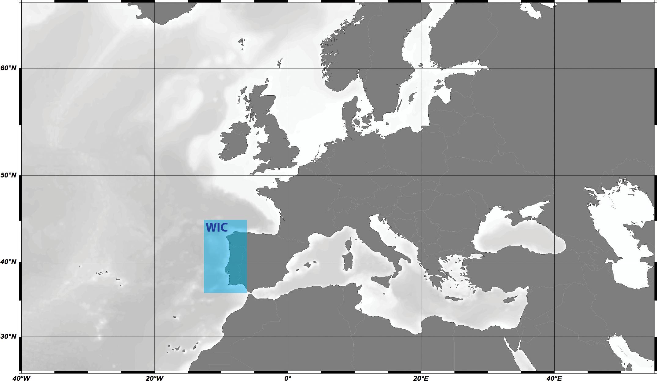
Figure 1. Location of the Western Iberian Coast (WIC).
Western Iberian Coast is inserted in the Northern Canary Current System, one of the four major Eastern boundary upwelling systems worldwide (Wang et al., 2015). Upwelling off the WIC is highly seasonal, with higher intensity during the boreal summer (Wooster et al., 1976; Fiúza et al., 1982; Lemos and Pires, 2004), particularly off upwelling centers (e.g., off Galiza and Sagres). The influence of the nutrient input driven by upwelling on the marine phytoplankton off the WIC has been thoroughly studied for several regions within the WIC (e.g., Tilstone et al., 2003; Ribeiro et al., 2005; Rossi et al., 2013; Goela et al., 2014). Other significant agents in this region include several large river basins along the coast (e.g., Tagus, Douro, Guadiana, Guadalquivir), which deliver valuable nutrient inputs for coastal phytoplankton communities. Moreover, WIC’s proximity to the mouth of the Mediterranean Sea has been seen to shape nearby biological communities (González-García et al., 2018).
Biological Data: Satellite Chlorophyll a
Weekly surface CHL remote-sensing data (L4 with 1 km spatial resolution) for the WIC were acquired from the North Atlantic CHL concentration from satellite observation (daily average) Reprocessed L4 (ESA-CCI); available at http://marine.copernicus.eu/ for the period 1998–2016. This product is derived from merging Remote Sensing Reflectance (RRS) data from three different sensors: Sea-viewing Wide Field-of-view Sensor (SeaWiFS), Moderate Resolution Imaging Spectroradiometer-Aqua (MODIS-Aqua), and Medium Resolution Imaging Spectrometer (MERIS). Subsequently, CHL is estimated by applying the OC5ci algorithm, which combines algorithms OC5 (Gohin et al., 2002), for coastal waters, and OCI (Hu et al., 2012) for the open ocean. This dataset is already optimized for the NE Atlantic, displaying a good agreement with the in situ measurements (R2 = 0.79; RMSE = 0.26) and spatial coverage of about 95%. Moreover, an intercomparison effort of ESA-CCI derived-CHL (albeit an earlier version of the product) with in situ data from WIC was done by Sá et al. (2015). They reported values of unbiased root mean square error, standard deviation, and correlation coefficient that were comparable to other products, such as MODIS OC3M chlorophyll algorithm. Coastal pixels less than 4 km from the shore were excluded to avoid difficulties associated with nearshore Case II waters, such as CHL overestimation in the presence of colored dissolved organic matter (CDOM) and total suspended matter (TSM).
Mean and seasonal (i.e., mean for each annual season) CHL climatologies for 1998–2016 were calculated. CHL anomalies were also determined by detrending (i.e., removing the least-squares trend) the CHL time series and subsequently by deseasonalizing (i.e., removing the mean associated with each month) it. The linear trend was obtained by calculating the slope of the least square regression model. Thus, the resulting anomalies are also independent of the seasonal variability and are genuinely representative of anomalous CHL variability.
Physical and Biogeochemical Data
Daily sea surface temperature data (SST; 4 km spatial resolution) for the period 1998–2016 were extracted from the Advanced Very High-Resolution Radiometer (AVHRR) Pathfinder SST product (PFV53; available at www.nodc.noaa.gov; Casey et al., 2010; Saha et al., 2018). This product is produced by the National Oceanic and Atmospheric Administration (NOAA) National Centers for Environmental Information (NCEI) and uses data from the AVHHR instruments aboard NOAA’s series of polar satellites. This dataset is considered highly reliable particularly due to its corresponding global multi-year in situ validation matchup dataset and has been utilized in several oceanographical studies off WIC (Santos et al., 2012; Alves and Miranda, 2013). Plus, only pixels flagged with quality level flags 6 and 7 (i.e., having passed all or almost all quality tests) were chosen to ensure the highest data quality (Kilpatrick et al., 2001).
1998–2016 ∼8 km spatial resolution weekly model-derived data on mixed layer depth (MLD; m), SAL (psu), sea surface height (SSH; m), and the zonal (U) and meridional (V) components of surface water flow (m s-1) were also acquired, from CMEM’s Atlantic – Iberian Biscay Irish (IBI) – Ocean Physics Reanalysis Product (IBI_Reanalysis_PHYS_005_002; available at http://marine.copernicus.eu/). The water flow velocity (WVel; m s-1) was also calculated from the U and V components. This product is based on the NEMO v3.6 ocean general circulation model (Madec, 2008) and forces the model with regional atmospheric fields available at the European Centre for Medium-Range Weather Forecasts (ECMWF)1 to ensure its optimization to the IBI region. This model has the advantage of assimilating in situ temperature and SAL data, as well as satellite SST and altimeter data. It has recently been validated for the IBI region using several surface and mooring buoys along WIC (for more details, see Levier et al., 2014, 2015; Sotillo et al., 2015).
Dissolved inorganic nitrogen (DIN; μM), calculated as the sum of nitrate (NH4) and ammonium (), phosphate (; μM), and silicate (Si) (μM) for the period 2002–2014 were acquired, with a weekly periodicity and 8 km spatial resolution, from CMEM’s Atlantic – IBI – Ocean Biogeochemistry Non-Assimilative Hindcast Product (IBI_Reanalysis_BIO_005_003; available at http://marine.copernicus.eu/). This product uses both the ocean physical IBI reanalysis product mentioned above and the biogeochemical model PISCES (Levier et al., 2014) to derive a 3D high-resolution product with several biogeochemical variables optimized to the IBI region. In situ validation efforts have delivered good results, particularly for nitrates and phosphates (R2 > 0.75; RMSE = 2.04 and 0.1 for nitrates and phosphates, respectively; Bowyer et al., 2018). L3 weekly Photosynthetic Active Radiation (PAR; Einstein m-2 day-1) with a spatial resolution of 4 km was acquired, for the period 1998–2016, from the GlobColour project website (http://www.globcolour.info/; Frouin et al., 2003).
Climate Indices
Due to their relevance for the understanding of global and regional ecosystems in the North Atlantic, the following climate indices were obtained for 1998–2016: the NAO index, the East Atlantic (EA) pattern, the AMO, the Multivariate El-Niño/Southern Oscillation Index (MEI), and the Western Mediterranean Oscillation (WeMO). NAO, EA, AMO, and MEI were acquired from NOAA, while WeMO was acquired from the Climatology Group of the University of Barcelona.
All of the chosen climate indices have been seen to influence the climate over the NE Atlantic region (e.g., de Castro et al., 2008; Hurrell et al., 2013; Krug et al., 2017; Jiménez-Esteve and Domeisen, 2018). NAO reflects differences in atmospheric surface sea-level pressure in the North Atlantic Ocean between the subtropical high and subpolar low. Its positive phases are usually linked with high SSH and pressure and low precipitation and temperatures over Southern Europe (Hurrell et al., 2013). EA is similar to NAO in its calculation and is considered the second main variability pattern in the North Atlantic. EA, in its positive phase, is associated with higher temperatures and low precipitation across Southern Europe (Iglesias et al., 2014). AMO is a multidecadal SST-based index known for its importance to decadal-scale events, such as rainfall patterns and hurricane activity. While AMO has been under a constant positive phase since the 1990s, recent studies have found that AMO has become slightly negative the last few years due to cold anomalous SST values in the subpolar region and is expected to maintain its negativity (Frajka-Williams et al., 2017). MEI is closely related to ENSO, considered one of the most critical interannual climatic phenomena worldwide. Despite its intrinsic relation to the Eastern Pacific Ocean, ENSO has been observed to impact North Atlantic climate, such as interacting with NAO (Jiménez-Esteve and Domeisen, 2018). WeMO is a somewhat new pattern identified for the Western Mediterranean basin and its vicinities (Martin-Vide and Lopez-Bustins, 2006) and it is correlated primarily with rainfall patterns over the Iberian Peninsula (Martin-Vide and Lopez-Bustins, 2006).
Data Analyses
Prior to data analyses, the dataset was transformed to match the required temporal and spatial resolution, as needed. Linear relationships between CHL anomalies and environmental variables were assessed using Pearson correlations. Additionally, empirical orthogonal function (EOF) analysis (Lorenz, 1956) was used to identify and study spatio-temporal patterns of CHL variability along the WIC. Generalized additive models (GAMs) were used to identify and evaluate the effect of several environmental predictors on CHL variability.
Empirical Orthogonal Function (EOF) Analysis
Empirical orthogonal function analyses are often used in climate studies and can be very useful to understand the variability of a given variable, as it breaks a complex signal by delivering mathematically independent spatio-temporal modes and how these modes vary. However, despite its usefulness, EOF modes are not necessarily related to climate patterns and should be interpreted carefully. In this study, conventional EOFs (i.e., unrotated) were used. Rotated EOF analyses (e.g., varimax rotation; Kaiser, 1958) were also tested but were seen to worsen the interpretability of the modes and were thus discarded. To run the EOF analysis, a complete matrix corresponding to the response variable must be provided. Thus, CHL was averaged monthly, and the remaining missing data were filled following Racault et al. (2014) procedure, i.e., a moving mean with 3-pixel-size window was sequentially run longitudinally, latitudinally, and over time. After this procedure, the remaining missing data were residual (<0.01%). A final moving mean with a 3 × 3 pixel-size window was run to fill the remaining pixels as in Krug et al. (2017). Afterward, CHL was detrended and deseasonalized before applying the EOF analysis.
The EOF analysis allowed the extraction of variability modes from the CHL dataset into a spatial and temporal component. The significance of the resulting EOF modes was evaluated according to the method described by North et al. (1982). According to this method, an EOF mode is considered significant if its sampling error is smaller than the difference between the mode’s explained variance and the next mode [see North et al. (1982) for more details]. The resulting modes were used to identify regions with coherent CHL variability along the WIC using a similar methodology to Krug et al. (2017). The spatial component partitions WIC according to the spatial patterns of the mode, where negative and positive areas correspond to deviations regarding the mean of the mode over the dataset period, as further described in the section “EOF Analysis.” These negative/positive areas are considered as CHL-coherent regions, in terms of their own variability patterns and are considered to be out-of-phase in relation to each other.
Generalized Additive Models (GAMs)
Generalized additive model techniques were applied to evaluate the environmental drivers of CHL variability. GAMs are an extension of generalized linear models (GLMs), whereas the relationship between the response variable and the predictors can be non-linear. Thus, GAMs are more suitable for complex situations where nonlinear patterns may arise which would be missed or wrongly interpreted in a GLM. As such, it has been used extensively to study CHL drivers (e.g., Jayaram et al., 2013; Krug et al., 2017; Liu et al., 2017). In the present study, GAMs were applied to CHL anomalies within each region of coherent CHL variability patterns identified through the EOF analyses. GAM results were checked for residual autocorrelation and, since no significant evidence of autocorrelated was found, no autocorrelation structure was added to the GAM function. Simple linear correlations between each environmental variable were used as a screening procedure to exclude variables with high co-correlation (R2 > 0.7). GAM analyses were performed using the package mgcv 1.8-24 (Wood, 2006, 2017), in R (R Development Core Team, 2018).
Results
CHL and Environmental Climatologies
From the average CHL concentration during 1998–2016 (Figure 2), several coastal CHL hotspots can be identified along the WIC: off the Galician Rias (∼42.5°N), off most Northern and Central Portuguese coast (∼41.5°N–40°N), off the mouth of the Tagus estuary (∼38.5°N) and in the Cádiz Gulf (37°N, -8°E to -6°E). Several CHL plumes extending over several kilometers off the coast can also be found facing major estuaries or over the Estremadura Spur (∼39°N) and Aveiro region (∼39.5-40.5°N), where the continental shelf is wider. Overall, the average CHL distribution off WIC (Figure 2E) can be divided into two gradients: (i) an offshore south–north gradient, with lower mean CHL concentrations (<0.2 mg m-3) below 37°N and increasingly higher concentrations toward the Northern latitudes of WIC (e.g., ∼0.4 mg m-3 circa 45°N); and (ii) an offshore–inshore gradient, with mean CHL over 1 mg m-3 next to the coast. Moreover, results suggest that CHL in the WIC displays a marked seasonality, typical of temperate waters (Figures 2A–D). Higher CHL concentrations in oceanic waters off the WIC were typically detected during the timing of the spring bloom. During summer, however, CHL is distinctively higher in the coastal area, when compared with other seasons, due to the influence of upwelling. An exception would be the Gulf of Cadiz region, where CHL is higher nearshore during spring as opposed to summer. Trend analysis revealed a general weak positive linear trend over the WIC (Figure 2F). CHL trends over 0.02 mg m-3 year-1 were found off the northWestern coast. Nonetheless, a negative trend was observed on the Southern coast, particularly in the Cadiz Gulf, where values under -0.06 mg m-3 year-1 were found. While these can be considered weak trends, it is essential to think of these values as yearly trends that, at specific locations, may accumulate over a 19-year dataset.
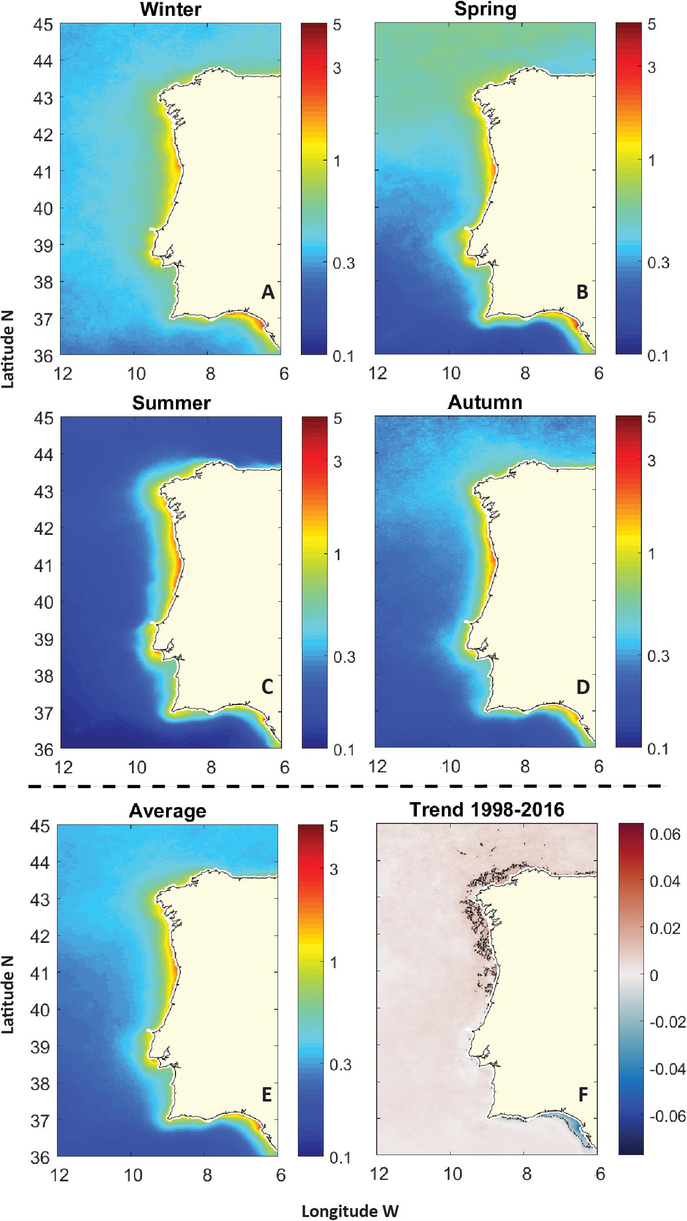
Figure 2. Climatologies (mg m-3) for the period 1998–2016 of: (A) winter CHL; (B) spring CHL; (C) summer CHL; (D) autumn CHL; and (E) CHL averages. The annual trend (mg m-3 year-1) observed during the period of the study is also presented in (F).
During 1998–2016, WIC presented itself as a highly complex region regarding its environmental forcing. Nutrient-wise, while higher concentrations were expectedly observed closer to the coast, each nutrient (DIN, , Si, and Fe) shows distinct patterns over the WIC. High mean DIN concentrations (>5 μM; Figure 3A) were found in the coastal zone of the WIC, mainly between 38°N and 43°N. Nevertheless, a clear offshore latitudinal gradient can be seen, as DIN increases toward higher latitudes. A similar pattern can be observed for phosphate (; Figure 3B). However, relatively high mean phosphate concentrations (>0.3 μM) were also observed on the Eastern Gulf of Cádiz (off the Guadalquivir estuary mouth and Cádiz). Si are mainly concentrated on the coastal zone of the WIC (38°N–43°N) and off the Eastern Gulf of Cádiz, where it reached mean concentrations over ∼7 μM (Figure 3C). Mean iron (Fe) concentrations were mainly higher along the coast (>3 × 10⁻³ μM), while also displaying a north–south decreasing gradient (Figure 3D). Mean SST ranged from ∼15 to 19°C along the WIC (Figure 3E). Overall, SST was seen to be higher toward Southern latitudes. However, a cold coastal southward plume caused by coastal upwelling and coastal currents can be seen along the Western coast with temperatures below 17°C. MLD also varied considerably over the study area, ranging from <15 m on coastal areas to >40 m offshore (Figure 3I). The highest MLDs were detected north of 43°N (>50 m). PAR analysis revealed almost a linear north–south gradient toward the Southern region WIC, ranging between 29 and 39 einstein m-2 day-1 (Figure 3F). Mean SAL across WIC was generally above 35.5 psu, except at some coastal areas that are strongly influenced by riverine inputs (e.g., off Northern Portugal) where salinities as low as ∼34 psu were detected (Figure 3G). Mean SSH, from 1998 to 2016, ranged between -0.3 and -0.38 m. Lower heights were typically detected on coastal areas around 43–45°N, while higher values were seen in oceanic waters below 39°N (Figure 3H). Mean water flow components and speed (Figures 3J–L) show that water along the WIC typically flows southward, while along the Southern coast it flows eastward near the coast and westward in the Southern offshore areas. From 39°N to 42°N, water can be seen flowing slightly toward offshore, a sign of upwelling. Several regions where surface water flow speed averaged over 0.15 m s-1 were detected: off Peniche (∼39.3°N), off Sagres (∼37°N), and the Gulf of Cádiz, flowing into the Gibraltar Strait (36–37°N), where maximums over 0.3 m s-1 were measured.
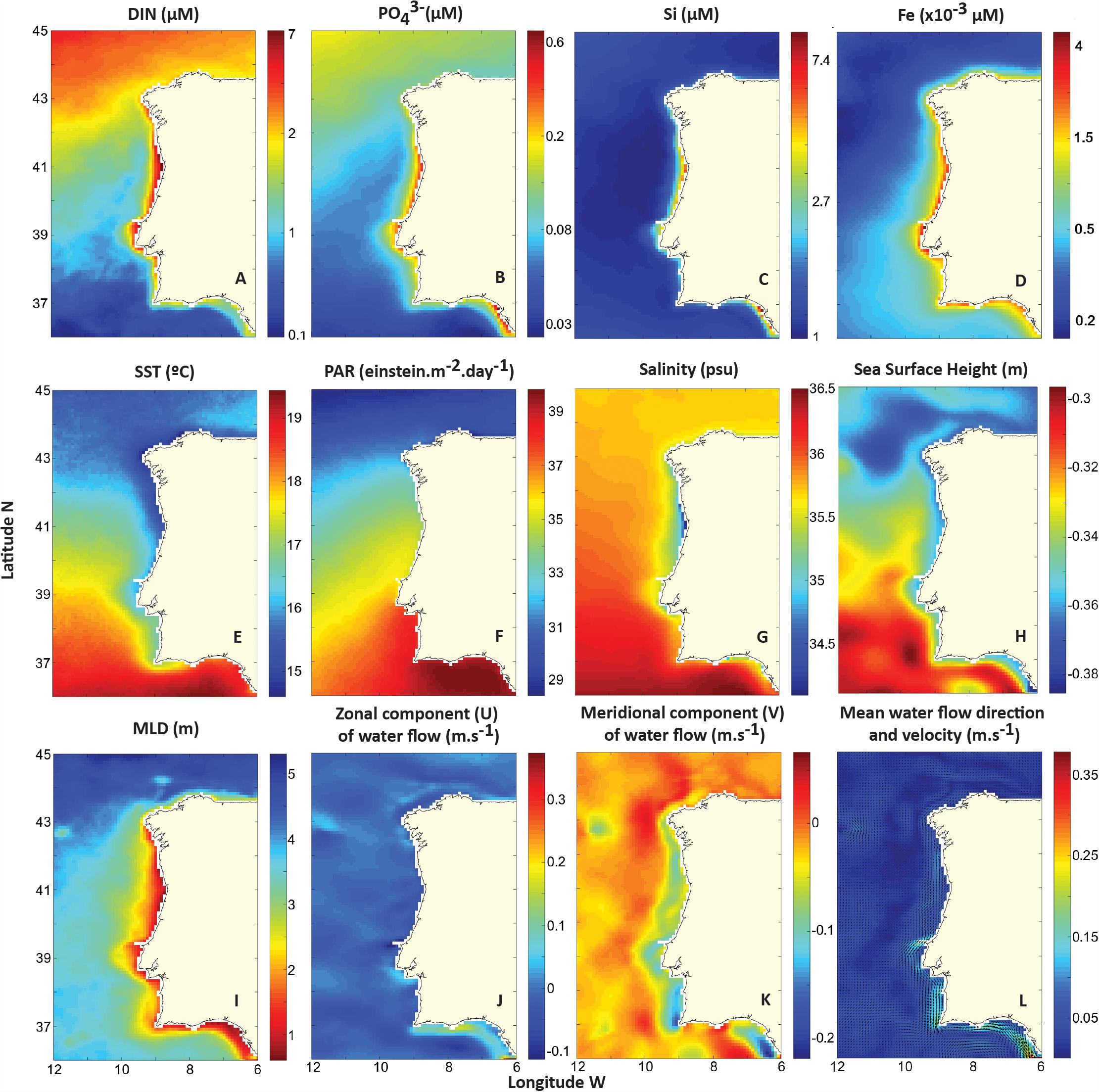
Figure 3. Mean environmental parameters in the WIC: (A) Dissolved inorganic nitrogen (DIN; μM); (B) phosphate (; μM); (C) Si (μM); (D) iron (Fe; ×10-3 μM); (E) sea surface temperature (SST; °C); (F) photosynthetic active radiation (PAR; einstein m-2 day-1); (G) salinity (psu); (H) sea surface height (SSH; m); (I) mixed layer depth (MLD; m); (J) zonal component (U) of water flow (m s-1); (K) meridional component (V) of water flow (m s-1); and (L) mean water flow direction and velocity (m s-1).
North Atlantic Oscillation index (Figure 4A), from 1998 to 2016, exhibits high variability, typically varying interannually between positive and negative phases. Nonetheless, three major positive (1999–2001, 2012, and 2013–16) and two negative (2009–2011 and 2013) periods may be detected. The AMO has remained mostly positive since 1998 (Figure 4B), fluctuating between 0 and 0.5. Otherwise, only a few minor negative episodes were recorded over the studied period (e.g., 2009). The East Atlantic (EA) pattern index (Figure 4C) was mostly positive, with one long positive period between 2000 and 2004 followed by two short positive instances centered in 2007 and 2010. Since 2012, EA has been increasingly positive with rare negative episodes. The El-Niño/Southern Oscillation Index (MEI) fluctuations over the years indicate several El-Niño events between 1998 and 2016 (Figure 4D). Strong El-Niño events occurred in 1998 and 2014–16, while weaker El-Niño followed by strong La-Niña events occurred in 2006–7 and 2009–10. Regarding the WeMO index, apart from a small period between 2000 and 2002, was seen to be on a steady negative phase (Figure 4E). Negative peaks were detected in 2006 and 2011.
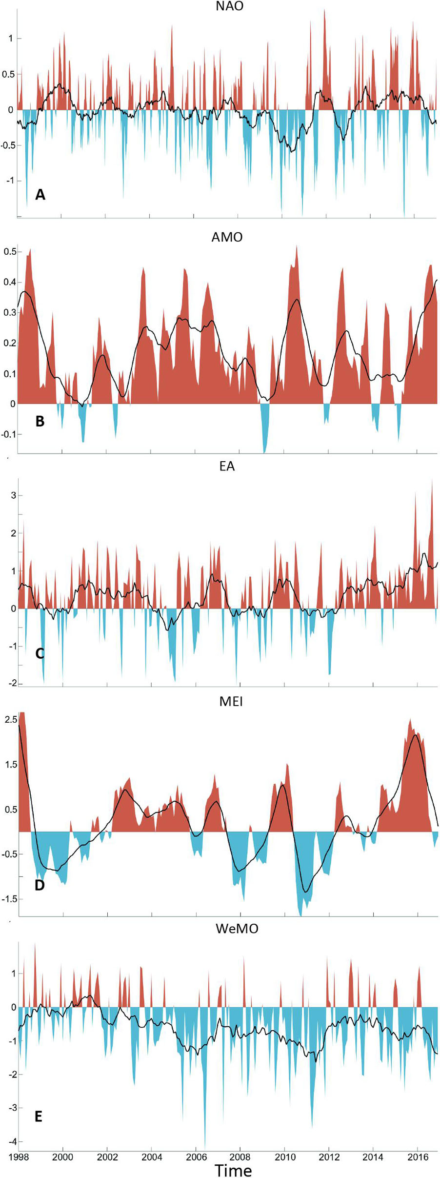
Figure 4. Temporal variability of climate indices, from 1998 to 2016: (A) North Atlantic Oscillation (NAO), (B) Atlantic Multi-decadal Oscillation (AMO); (C) East Atlantic (EA) pattern; (D) Multivariate El Niño-Southern Oscillation (MEI); and (E) Western Mediterranean Oscillation (WeMO). Black lines represent 3-month moving means.
Correlation Analysis
Linear relationships between CHL anomalies and environmental variables included in this study are presented for the entire period of the datasets (1998–2016; Figure 5). Several relevant significant linear relationships were identified for some areas off WIC, a summary of the most relevant is described in Table 1. Nitrogen (DIN) and phosphates () yielded a significant positive correlation with CHL anomalies, especially along coastal areas, as well as on the offshore area located under 40°N. These positive relationships suggest a direct driver–response relationship at those specific areas. Interestingly, higher negative correlations between SST and CHL anomalies were seen around Sagres, a known upwelling center in WIC.
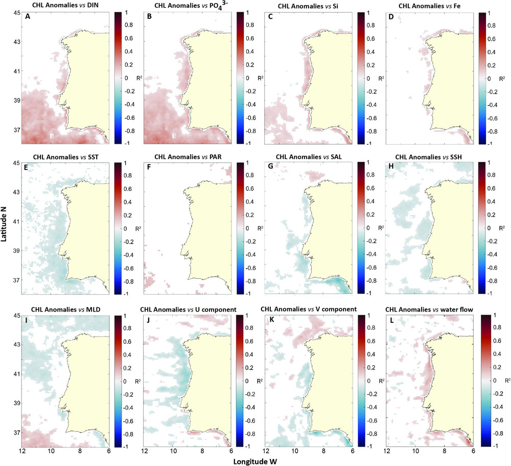
Figure 5. Spatial distribution of significant correlations (p-value < 0.05) between CHL anomalies and: (A) DIN (μM); (B) phosphate (; μM); (C) Si (μM); (D) Fe (× 10-3 μM); (E) SST (°C); (F) PAR (einstein m-2 day-1); (G) salinity (psu); (H) SSH (m); (I) MLD (m); (J) zonal component (U) of water flow (m s-1); (K) meridional component (V) of the water flow (m s-1); and (L) mean water flow velocity (WVel; m s-1).
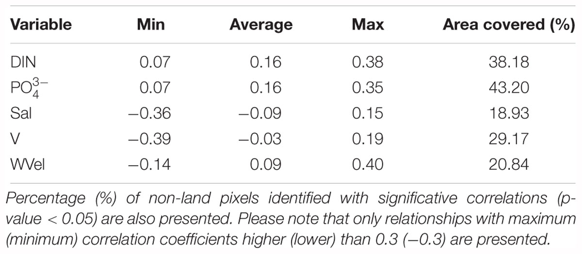
Table 1. Minimum, average, and maximum correlation coefficients observed between the environmental variables and CHL anomalies.
Salinity exhibited an inverse relationship with CHL anomalies along the Western and Southern coast of the Iberian Peninsula, most likely as a result of nutrient-rich river discharges. Correlations were particularly strong in the Gulf of Cadiz, suggesting river discharges might have a big role in CHL variability here. However, SAL did correlate positively with CHL anomalies over a patch north of Galicia, also suggesting differences in CHL anomalies patterns. The surface water flow indices (U and V) exhibited mostly negative correlations off the West coast and several positive correlated patches above 43°N (Figures 5J,K). Their main distinction occurred off the Southern coast and Gulf of Cadiz, where positive coefficients were identified between CHL anomalies and U, while negative coefficients were seen for V. The mean WVel showed positive correlations with CHL anomalies off the Western and Southern coast. The difference in linear correlations between U and V over WIC is a testament to the importance of wind-driven coastal processes such as upwelling, in this area. Negative correlations between U and V and CHL anomalies along the Western coast of the Iberian Peninsula indicate SW-oriented water transport, highly associated with coastal upwelling in WIC, contributes to higher CHL. Overall, this heterogeneity suggests different patterns of CHL variability over WIC, with distinct environmental drivers being responsible, underlining the importance of the regionalization process utilized in this study.
EOF Analysis
Empirical orthogonal function analysis returned six statistically significant modes. Overall, these six modes explained a total of 57.6% of the total extant variance. Despite these six significant modes, only the first four modes (∼51.7% of the total variance) were further contemplated and analyzed to avoid overcomplexity. Figures 6A–D display the first four modes produced by the EOF analysis, including their spatial mode and the temporal variability for each mode, from 1998 to 2016. Mode 1 explained 28.75% of the total variance and its spatial component is mostly positive over WIC, meaning most WIC displays a similar variability pattern according to this mode. Moreover, offshore values were typically higher, except in a few negative zones, located on the Southern coast, particularly off Cádiz (Figure 6A), where the variability pattern was different. Regarding its temporal variability, it is clear that there are consistent negative peaks during early spring, while positive peaks showed no apparent seasonality, occurring irregularly during summer, autumn, and winter (Figure 6A). However, their magnitude is inconstant, particularly of the positive phases, as major peaks were identified in 2005 and 2009. Interestingly, 2016 was the only year where mode 1 did not change its signal, remaining negative throughout the year. Overall, this mode appears to be capturing, on its negative phase, CHL anomalies during the timing of the typical Northeast Atlantic temperate spring bloom. Mode 2 explained circa 12% of the total variance and displayed a very distinct spatial component than mode 1 (Figure 6B). According to mode 2, two main contrasting areas can be found: a positive area north of 41°N, excluding a coastal strip off Western Galicia, and a negative area occupying most of the area south of 41°N. Nevertheless, small areas varying positively with mode 2 were also identifying off the Douro and Guadalquivir estuaries. Mode 2 temporal component is complex and does not suggest any apparent seasonality. Regarding the temporal component, it is highlighted by two strong peaks: a negative peak during late winter of 2009 and a positive one during mid-spring of 2011. Mode 3 (Figure 6C) is responsible for explaining 6.36% of the total variance and, similarly to mode 2, also defines two main large areas over WIC with contrasting signals. On the one hand, a positive area encompasses most of the Iberian coastline and a sizeable oceanic patch between 39°N and 43°N. On the other hand, the offshore waters above 43°N and under 39°N may be observed to vary negatively with mode 3. Two main negative periods, with peaks during the spring of 2004 and 2012, highlight the temporal component of this mode. Intriguingly, the two main positive peaks of mode 3 appear to occur immediately after these negative periods, also during spring (2005 and 2013). Lastly, mode 4 (Figure 6D) explains 4.52% and has the most complex spatial and temporal components of the four considered EOF modes. Spatially, it appears to divide WIC longitudinally, resulting in a positive oceanic area east of -10°E and a broad negative more coastal area, with lower negative values alongshore. This pattern suggesting its variability is related to coastal processes. Two main positive peaks were identified in 2009 and 2015, while, at least, three major negative peaks occurred in 2001, 2009, and 2016.
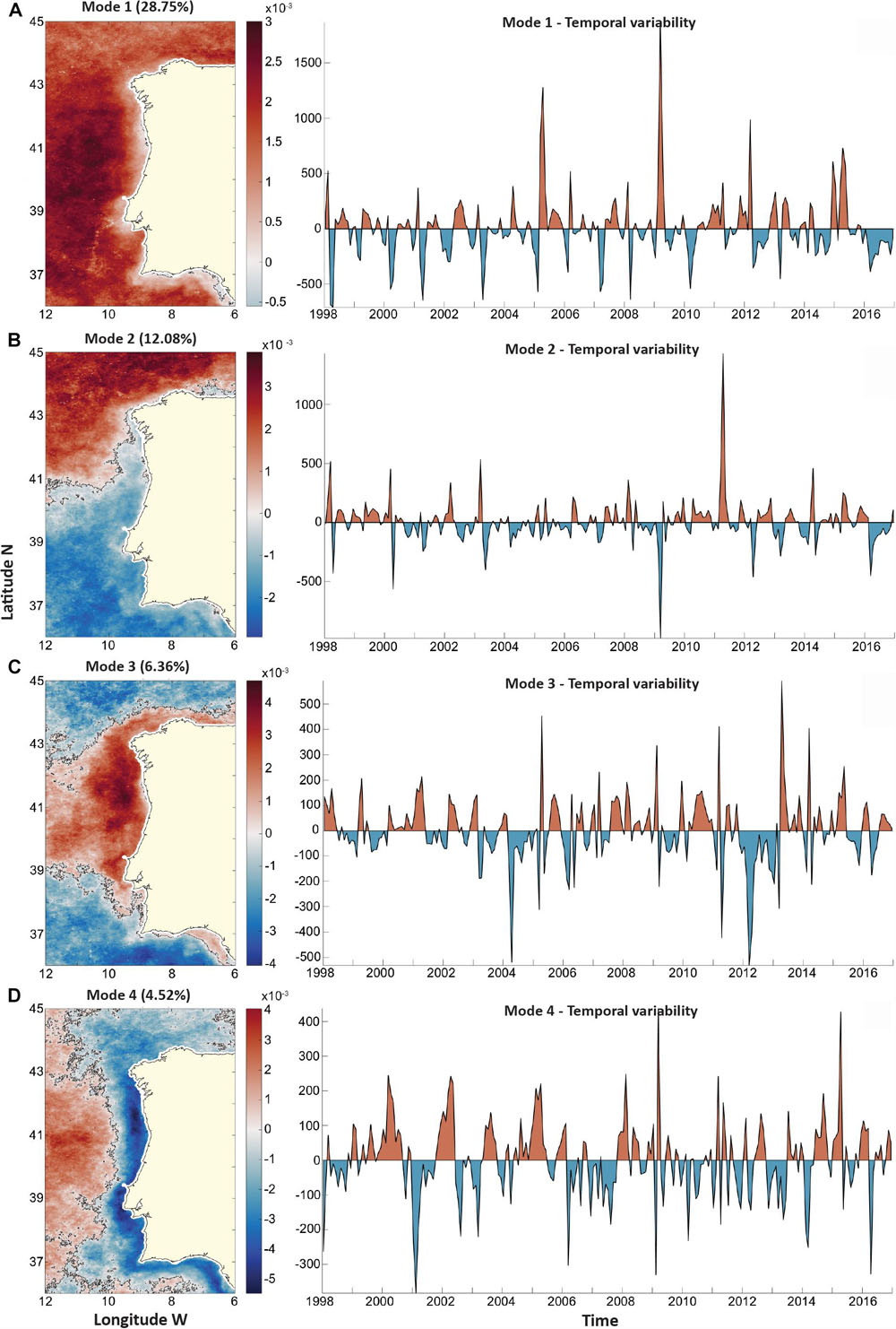
Figure 6. Empirical orthogonal function (EOF) analysis for the WIC region, covering the years from 1998 to 2016. Spatial component and time-varying amplitude coefficients are presented side by side for: (A) First EOF mode (EOF1) that explained 28.75% of total variance; (B) second EOF mode (EOF2) that explained 12.08% of total variance; (C) third EOF model (EOF3) that captured 6.36% of total variance; and (D) fourth EOF mode (EOF4) that explained 4.52% of total variance.
Using the spatial components from EOF modes 1–4, six areas with coherent CHL variability over WIC were defined (Figure 7 and Table 2). First, the positive/negative areas for the first four modes were combined, as shown in Table 2. As a result, 16 (all) possible combinations were produced, 5 of which returned no pixels. Subsequently, linear correlations were performed on the CHL anomalies of the remaining 11 areas to avoid redundancy. Areas geographically next to each other with high correlation (R2 > 0.85) were merged, resulting in six regions with distinct chl a variability patterns (Table 2). Half of the regions were oceanic, while the other half were mainly coastal, revealing sharp differences between coastal and oceanic CHL variability. Overall, each designated region appears to be associated with distinct CHL variability patterns and, as seen by the subsequent GAM analyses, associated with distinct environmental drivers.
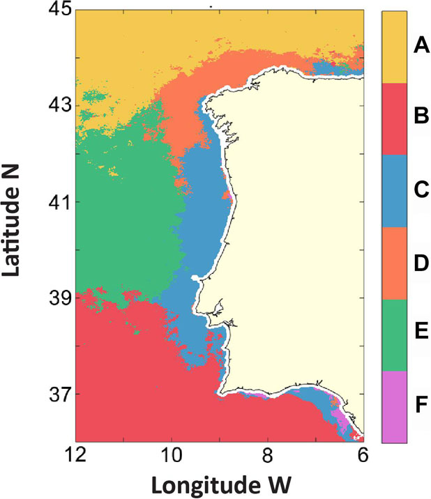
Figure 7. Regions with similar CHL variability patterns (from 1998 to 2016) for the Western Iberia Coast (WIC), derived by combining the positive and negative signals of the EOF spatial components used (EOF1, EOF2, EOF3, and EOF4), according to the scheme presented in Table 2.
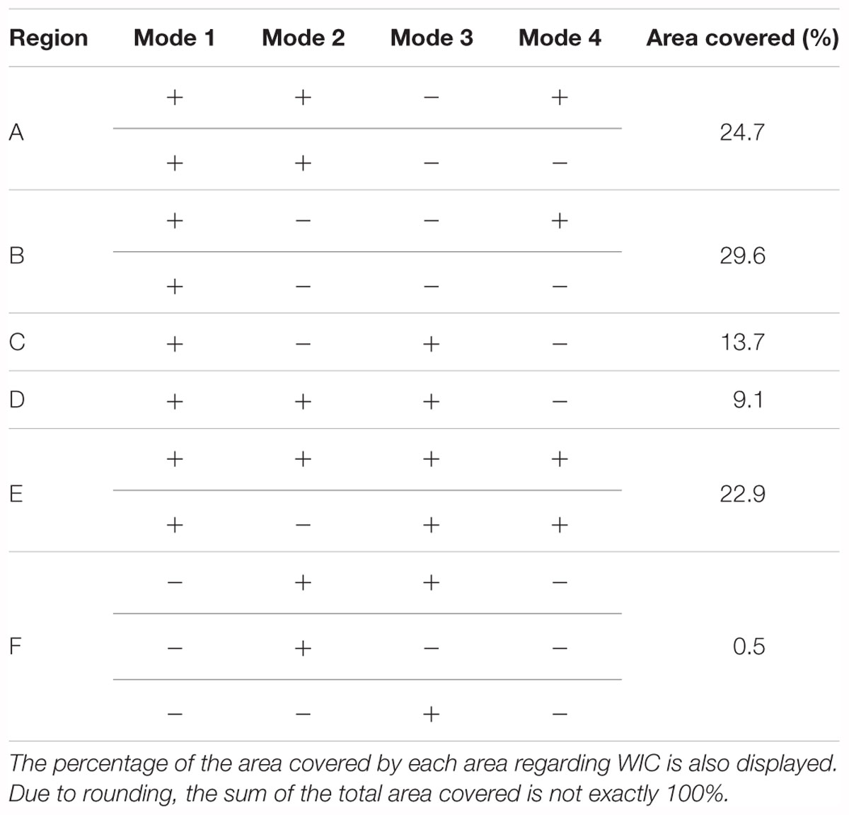
Table 2. Summary of the creation process leading to the regionalization of WIC in six CHL coherent regions using the positive and negative signal of the modes resulting from the EOF analyses.
Region A is located in the Northern region of WIC, ranging from 43°N to 45°N, coinciding almost entirely with the negative Northern area observed in the spatial component of mode 3. This area is mainly oceanic. Region B, the largest region defined in this study, is also mostly oceanic, located in the Southern part of the WIC region, but it also includes small portions of the Southern coast. Region C covers most of the coastline, except in the Northern part of Galicia. Region D is mainly composed of the coastal zone in the northWestern part of Galicia, yet it also includes several small zones off the mouths of the Douro and Guadalquivir estuaries (corresponding to the positive areas defined by mode 2; Figure 6B). Region E occupies a sizeable oceanic area off central WIC, extending roughly from 39°N to 42°N. Region F is the smallest region created (0.5% of the study region), coinciding with the areas with negative values in the spatial component of Mode 1.
GAM Analyses
Results of the GAM analyses, which identified the most important environmental drivers, are presented in Table 3. Each significant model predictor is identified, as well as its degree of significance. The model’s adjusted R2 and explanatory power (i.e., variance explained) are also provided. Plus, the partial effects of the main detected predictors on CHL anomalies are exhibited in Figure 8 for each region, using a schematic display. An additional figure with all the results is provided as Supplementary Material.
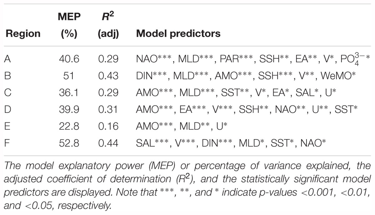
Table 3. Summary of the best performing generalized additive models (GAM) performed on the effects of environmental predictors on CHL anomalies of each of the specific regions derived by combining the signal of the EOF spatial component.
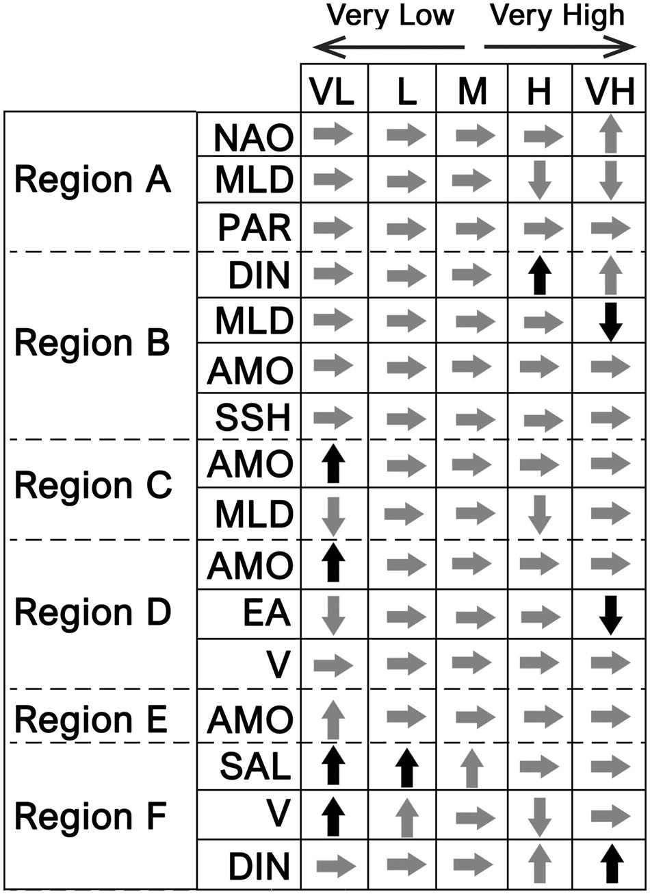
Figure 8. Partial effects of individual environmental predictors, derived from the best performing GAM, on CHL anomalies of each region (A–F). Only the main significant predictors are shown (p-value < 0.001). Arrows display the change on CHL anomalies associated with very low (VL), low (L), high (H), and very high (VH) values of the predictor. M corresponds to the midpoint in the range of observed values. Arrows facing up (down) indicate positive (negative) CHL anomalies, while arrows facing right indicate near-zero anomalies. Gray arrows indicate a small-to-medium increase in CHL anomalies, while black arrows indicate a large increase (see also Figure 9).
Overall, AMO, MLD, and V were the most common environmental predictors identified by the GAM analyses, being present in most of the models. Other common predictors were DIN and NAO. These results show that despite WIC spatial complexity, there is a set of main environmental drivers that contribute to the CHL variability in most regions (Figures 8, 9). Nonetheless, each model indicated a unique combination of significant environmental predictors. The variability of CHL anomalies in region A was seen to be explained by NAO, MLD, PAR, SSH, EA, V, and (40.6% of the total variance explained). Results suggest very high values of the NAO index are associated with positive CHL anomalies. In addition, high MLDs were seen to be paired with negative anomalies. Such results are expected since a shallow or warmer mixed layer contribute to bloom initiation in the Northern Atlantic (Cole et al., 2015). PAR, while being a significant predictor of CHL in this region, did not appear to have a clear association with either positive or negative CHL anomalies. GAM model for region B yielded a wide suite of environmental predictors responsible for CHL variability: DIN, MLD, AMO, SSH, V, and WeMO. Among these, DIN, MLD, AMO, and SSH were considered the most significant. DIN, in particular, is suggested to have a large effect on CHL on region B, as relatively high concentrations were linked to strong positive CHL anomalies. High MLDs exhibited the opposite effect on CHL, i.e., causing negative anomalies. AMO and SSH revealed no clear trend toward either positive or negative anomalies. Concerning region C, GAM analysis identified seven significant predictors: AMO, MLD, SST, V, EA, SAL, and U, with AMO and MLD being the more relevant. Very high negative AMO index values (i.e., colder temperatures) were linked to strong positive CHL anomalies. This analysis also suggested negative CHL anomalies associated with both low and high values of MLD. For region D, the GAM model explained up to 39.9% of its total variance using AMO, EA, V, SSH, NAO, U, and SST as predictors. Similar to region C, very high negative AMO values are also strongly linked to strong positive CHL anomalies. Both strong negative and positive phases of the EA pattern were seen to cause negative CHL anomalies on region D, particularly during strong positive phases. No clear results were found for V. Region E was the region with the weakest model, only explaining circa 22.8% of its total variance. Unlike other regions, only three environmental variables were identified as drivers of CHL anomalies: AMO, MLD, and U. As with regions C and D, AMO was also fundamental, revealing a common pattern between these three adjacent regions. Region F was the region with the most powerful GAM (52.8% of the total variance explained). SAL, V, DIN, MLD, SST, and NAO were the predictors identified by the model, with SAL, V, and DIN being the most significant. SAL is clearly a relevant predictor in region F, located at Cádiz Gulf, as low-to-average values of SAL in this area are clearly associated with high positive anomalies. Positive CHL anomalies were also found to be related to high DIN concentrations. Moreover, very low and low (Negative) V was linked to CHL positive anomalies, indicating stronger north-to-south water transport, while positive values of V suggested a negative effect on CHL anomalies.
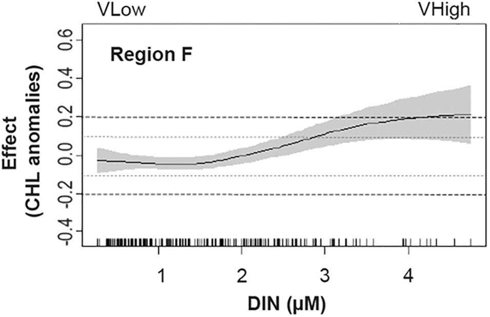
Figure 9. Partial effects of predictor DIN, derived from the best performing GAM for Region F. The solid line is the fitted model and the gray shaded areas represent the 95% confidence intervals. The actual observations of the predictor are represented on the x-axis. This plot illustrates how the schematic representation in Figure 9 was derived. Arrows facing up (down) in Figure 8 indicate that the predictor is associated to CHL anomalies above (below) 0.1 (–0.1) mg m-3 (represented by the gray dotted line). If the change (increase or decrease) is higher than 0.2 mg m-3, the arrow is black, otherwise it is considered a small-to-medium change (gray arrow).
Discussion
CHL Variability of WIC
Chlorophyll a was seen to be highly heterogeneous over the WIC region, both spatial and temporally. Four CHL coastal hotspots were identified: (1) off the Galician Rias, (2) off central-Northern Portugal, (3) off Tagus estuary, and (4) Gulf of Cádiz (Figure 2). On the first two, CHL is promoted by both local riverine nutrient input from local rivers with mixed average annual discharges (Hurrell et al., 2013) and coastal upwelling. Since these nutrient input sources are temporally independent (riverine input peaks during winter–spring, while upwelling occurs during summer–autumn), there is a sustained flow of nutrients almost all-year round. However, a recently identified declining trend in the intensity of coastal upwelling off northWestern Iberia (Pérez et al., 2010) may lead to a future decline in phytoplankton biomass and impact local ecosystems. Off the Tagus estuary, the situation is slightly different, as the major contribution to phytoplankton growth is likely to come from the Tagus riverine discharges. Nonetheless, this region is also influenced by coastal upwelling, which, due to its sheltered location, can lead to harmful algal blooms during relaxation (Moita et al., 2003). Finally, the Gulf of Cádiz is a complex basin mainly fueled by local freshwater discharges and its semi-enclosure, thus explaining why this is the only considered CHL hotspot where maximum concentrations are found on spring (as opposed to summer on the remaining regions).
Overall, the trend analysis suggests there are two regions where CHL appears to be heading separate ways. On the one hand, a positive trend was found in certain areas off Galicia and central-Northern Portugal. As seen above, this region is typically influenced by upwelling (Cravo et al., 2010; Pérez et al., 2010; Guerreiro et al., 2013; Wang et al., 2015; Vidal et al., 2017). Thus, it would be expected that such a positive trend would be linked to coastal upwelling. Several multidecadal studies have noticed upwelling off northWestern Iberia has become less intense the past 40 years (e.g., Pérez et al., 2010; Álvarez et al., 2011; Santos et al., 2011). However, trends in upwelling intensity may be contradictory as it is extremely reliant on factors such as the length of the considered time series, area, and season. Moreover, upwelling intensity is theoretically expected to increase according to future climate scenarios (Bakun et al., 2010; Wang et al., 2015) and recent studies have shown that upwelling off the WIC is no exception as local upwelling favorable winds are expected to increase during the XXI century (Casabella et al., 2014; Álvarez et al., 2017; Sousa et al., 2017). Since this study analyzed a recent period (1998–2016), the positive trend found for CHL over northWestern Iberia corroborates these studies. Overall implications of a positive CHL trend off northWestern Iberia would include a possible increase in productivity of exploitable species (e.g., small pelagic fish). On the other hand, a negative trend was detected off Southern Iberia, particularly on the Eastern Gulf of Cádiz. One reason for this could be the decrease in runoff of the main rivers located on the Gulf of Cádiz, such as Guadiana and Guadalquivir, which is only expected to worsen in the future (Estrela et al., 2012). Since the riverine nutrient input is the primary nutrient source of phytoplankton in the Gulf of Cádiz (Caballero et al., 2014), it would be expected for CHL concentration to diminish in response to lower discharges (Briceño and Boyer, 2010). Such a decline in CHL concentration could lead to impact local ecosystem processes and function (Winder and Sommer, 2012).
Disentangling CHL Variability: EOF Analyses as a Tool
Each one of the EOF modes exhibited different spatiotemporal patterns which help disentangle CHL variability along WIC during 1998–2016. Mode 1 captured the North Atlantic temperate spring bloom on the more oceanic areas, as these areas are less influenced by other factors that would mask this effect (e.g., upwelling, river discharges, anthropogenic pressure). This demonstrates the importance of the temperate spring bloom for the overall phytoplankton biomass variability over WIC. It also draws attention to the possible consequences of climate change on the magnitude and timing of the Northeast Atlantic spring bloom. For instance, several studies suggest that peak biomass, mean cell size, and diatoms relative abundance should decrease, leading to impacts on zooplankton feeding and, ultimately, to the efficiency of the food web (Sommer and Lengfellner, 2008; Sommer and Lewandowska, 2011), while others suggest a possible mismatch and decoupling between phytoplankton and zooplankton phenology (Edwards and Richardson, 2004).
Overall, mode 2 may be capturing phytoplankton response to the existent biogeochemical and physical meridional gradient between SW and NW Europe. WIC is considered as a transition area due to its climate. According to the Köppen–Geiger climate classification (Peel et al., 2007), the most widely used climate classification scheme, WIC can be divided into three temperate subclimates: temperate with a dry hot summer (36–40°N), temperate with a dry warm summer (40–42°N), and temperate without a dry season and a warm summer (42–44°N). While this classification is based on temperature and precipitation for terrestrial regions, this main change from a temperate climate with dry summer to one without a dry season is reflected on several marine properties. This is supported by the sharp differences across the 42–44°N strip observed for some environmental drivers in this study (e.g., SST, DIN, SAL, SSH, MLD, PO4, and PAR; Figure 3). Among the climate indices considered, NAO has been seen to be linked to differences in wind, temperature, and precipitation between SW and NW Europe (Hurrell et al., 2013). Thus, it is not surprising to see major NAO events (Figure 4) roughly reflected in the temporal variability component of mode 2. For instance, 2009–2010 winter NAO index was one of the most negative in recorded history, resulting in unusually high negative SST anomalies and temperatures over Europe (Osborn, 2011). Other recent negative NAO events can also be seen to generally correspond to negative peaks in the temporal component of mode 2 (e.g., 2012–13 and 2016). Also, there is a large positive peak mid-2011 that could correspond to a strong positive NAO phase in 2011–12. All in all, this mode underlines the importance of the influence of climate, mainly captured by NAO. Modes 3 and 4 correspond to much less variance explained, and, thus should be interpreted more carefully. One strong possibility for explaining the spatial cross-shelf positive–negative pattern seen for Mode 4 is that coastal nutrient input is driving this variability mode. Other studies have identified similar modes with cross-shelf patterns related to nutrient input (e.g., Tran et al., 2015; Krug et al., 2017; Liu et al., 2017), supporting this hypothesis.
All in all, most of the considered modes identified by the EOF analyses could be, at least, partly linked to known oceanographical processes. As EOF modes start to explain lower percentages of the total variance, their spatial and temporal components become more complex, resulting in a possible diminishing of the ecological meaning of modes (Navarra and Simoncini, 2010). Such may have happened with mode 3, resulting in a mode with unclear spatial and temporal components.
Environmental Forcing of CHL Anomalies in Selected Areas
Overall, coherent CHL-variability regions and its drivers were successfully identified for each region, providing relevant results for further understanding of CHL variability over WIC. GAM results suggest that physical processes and climate are the main factors that drive phytoplankton variability in Northern WIC, while in the Southern WIC, phytoplankton is more dependent on nutrient concentration. While nutrient availability is indeed linked to physical processes and climate, DIN, Si, and concentrations do not appear to be limiting phytoplankton in Northern WIC. Region E, interestingly, may be acting as a transition region between regions A and B, thus capturing characteristics from each region. AMO, the main significant predictor identified by the GAM model in region C, is known to be associated with changes in the Atlantic Meridional Overturning Circulation (AMOC; Wang and Zhang, 2013). AMOC influences the heat transport along the North Atlantic, and changes may lead to stronger heat transport and reduced precipitation over WIC (Pohlmann et al., 2004, 2009) that is likely to influence areas C, D, and E. Regarding regions C and D, CHL variability seems to be highly influenced by a combination of basin-wide (e.g., NAO, EA, AMO) and coastal processes (e.g., continental runoff, upwelling–downwelling). While they shared several significant predictors, unique predictors were also identified for each region. MLD and SAL are particularly relevant for region C, the second due to its nature as a proxy of riverine input. Regarding region D, CHL was seen to be linked with V (northward transport) and both very high negative and positive values of EA. Interestingly, since region D overlaps with the NW Iberian shelf, known for its upwelling, it would be expected for positive CHL anomalies to be associated with negative values of V, thus indicating upwelling-favorable winds, which was not observed. One possibility is that northward transport (positive V) may be associated with the Portuguese Coastal Counter-Current (PCCC). PCCC is a well-defined poleward surface current which may occur from September–October to February–May, typically associated with downwelling-favorable winds in the NW (Ambar and Fiúza, 1994; Álvarez-Salgado et al., 2003). During this period, when continental runoff is high, the subsequent plumes from the Galician Rías Baixas and Northern Portuguese rivers (e.g., Minho, Douro) contribute to the PCCC flow (Álvarez-Salgado et al., 2003; Ferreira Cordeiro et al., 2018). Consequently, this leads to shelf-wide mesotrophic conditions off NW Iberia due to the inflow of nutrient-rich waters (Álvarez-Salgado et al., 2003; Otero et al., 2008). Since region D width roughly matches NW Iberia’s shelf, the PCCC could be influencing GAM results as CHL positive anomalies during Autumn–Winter could be standing out. Finally, region F is a purely coastal region, and the results reflect that condition. SAL was the main driver, underlying the importance of riverine discharges in this region. This is underlined by the strong association found between high DIN concentrations and CHL anomalies. Negative V was also seen to drive positive CHL anomalies in this region, alluding to the coastal upwelling already seen in this region.
Overall, results suggest CHL variability over WIC is spatially heterogeneous and driven by a multitude of environmental agents. In more oceanic waters, CHL anomalies were seen to be associated with a suite of drivers (e.g., MLD, AMO, and NAO) possibly linked with basin-wide processes, such as the North Atlantic temperate spring bloom or the NAO. Meanwhile, for more coastal regions, upwelling and river discharges were seen to be important factors, with drivers such as SAL and the V and U components. Thus, WIC seems a highly complex area where CHL variability was seen to be highly heterogeneous with oceanic and coastal regions being associated with distinct drivers.
Final Remarks
Determining how environmental changes drive phytoplankton is essential for understanding oceanic and coastal ecosystems. This study sought to contribute to this matter by focusing on CHL anomalies over the WIC, assessing the most critical environmental drivers and the underlying patterns between them and CHL anomalies. For the first time, this was successfully achieved at the WIC scale, as this study identified not only the main modes of CHL variability over WIC but also regions with similar variability. This study, most of all, points out that complex areas such as WIC must be handled carefully under the context of environmental management and water quality, and that remote-sensing and modeled data are essential toward unraveling such complexity. The results of this and similar studies are essential for evaluating WIC under the EU MSFD subregion “Bay of Biscay and Iberian Coast,” contributing to the knowledge of CHL variability patterns for regions where in situ data are spatially and temporally scarce.
Nevertheless, some limitations should be taken into account: (i) the 19-year dataset here used might not be enough to analyze certain aspects of these complex processes (e.g., how AMO impacts CHL variability due to its multidecadal nature) and (ii) this study was based purely on remote sensing and modeling data, as in situ is scarce and temporally patchy over WIC. Future studies should pursue the use of complementary methodologies, integrating long-term in situ datasets with satellite and modeling data. This would be key to further understand how the phytoplankton community is affected by environmental drivers, especially in terms of: (i) bloom phenology (i.e., bloom timing, including the initiation, duration, and maximum levels); as well as (ii) the community composition and structure. A more in-depth comprehension of processes affecting the phytoplankton community is required to evaluate their implications on local food webs and to contribute to regional environmental marine policies and management strategies.
Author Contributions
The conceptual idea of the manuscript was developed by AB. AB also contributed to data analysis, decision making and manuscript preparation. AF and PG-A both worked on data acquisition and analysis. AF wrote part of the manuscript as well.
Funding
AB was funded by Fundação para a Ciência e a Tecnologia (FCT) Investigador Programme (IF/00331/2013). PG-A and AF also received support from Fundação para a Ciência e a Tecnologia (FCT) Investigador Programme (IF/00331/2013). This study also received further support from Fundação para a Ciência e a Tecnologia, through the strategic project (UID/MAR/04292/2013) granted to MARE.
Conflict of Interest Statement
The authors declare that the research was conducted in the absence of any commercial or financial relationships that could be construed as a potential conflict of interest.
Supplementary Material
The Supplementary Material for this article can be found online at: https://www.frontiersin.org/articles/10.3389/fmars.2019.00044/full#supplementary-material
Footnotes
References
Álvarez, I., Gomez-Gesteira, M., de Castro, M., Lorenzo, M. N., Crespo, A. J. C., and Dias, J. M. (2011). Comparative analysis of upwelling influence between the Western and Northern coast of the Iberian Peninsula. Cont. Shelf Res. 31, 388–399. doi: 10.1016/j.csr.2010.07.009
Álvarez, I., Lorenzo, M. N., de Castro, M., and Gomez-Gesteira, M. (2017). Coastal upwelling trends under future warming scenarios from the CORDEX project along the Galician coast (NW Iberian Peninsula). Int. J. Climatol. 37, 3427–3438. doi: 10.1002/joc.4927
Álvarez-Salgado, X. A., Figueiras, F. G., Pérez, F. F., Groom, S., Nogueira, E., Borges, A. V., et al. (2003). The Portugal coastal counter current off NW Spain: new insights on its biogeochemical variability. Prog. Oceanogr. 56, 281–321. doi: 10.1016/S0079-6611(03)00007-7
Alves, J. M. R., and Miranda, P. M. A. (2013). Variability of Iberian upwelling implied by ERA-40 and ERA-interim reanalyses. Tellus A 65:19245. doi: 10.3402/tellusa.v65i0.19245
Ambar, I., and Fiúza, A. F. G. (1994). “Some features of the Portugal current system: a poleward slope undercurrent, an upwelling related summer southward flow, and an autumn-winter poleward coastal surface current,” in Proceedings of the Second International Conference on Air-Sea Interaction and on Meteorology and Oceanography of the Coastal Zone, eds K. B. Katsaros, A. F. G. Fiúza, and I. Ambar (Boston, MA: American Meteorological Society), 286–287.
Bakun, A., Field, D. B., Redondo-Rodriguez, A., and Weeks, S. J. (2010). Greenhouse gas, upwelling-favorable winds, and the future of coastal ocean upwelling ecosystems. Glob. Chang. Biol. 16, 1213–1228. doi: 10.1111/j.1365-2486.2009.02094.x
Beardall, J., Stojkovic, S., and Larsen, S. (2009). Living in a high CO 2 world: impacts of global climate change on marine phytoplankton. Plant Ecol. Divers. 2, 191–205. doi: 10.1080/17550870903271363
Behrenfeld, M. J., O’Malley, R. T., Siegel, D. A., McClain, C. R., Sarmiento, J. L., Feldman, G. C., et al. (2006). Climate-driven trends in contemporary ocean productivity. Nature 444, 752–755. doi: 10.1038/nature05317
Bojinski, S., Verstraete, M., Peterson, T. C., Richter, C., Simmons, A., and Zemp, M. (2014). The concept of essential climate variables in support of climate research, applications, and policy. Bull. Am. Meteorol. Soc. 95, 1431–1443. doi: 10.1111/j.1600-0668.2011.00708.x
Bowyer, P., Dabrowski, T., Gutknecht, E., Lorente, P., Reffray, G., and Sotillo, M. G. (2018). Atlantic IBI-Iberian Biscay Irish- Biogeochemical Multi-year product IBI_REANALYSIS_BIO_005_003. Copernicus Mar. Environ. Monitor. Serv. 97.
Boyce, D. G., Lewis, M. R., and Worm, B. (2010). Global phytoplankton decline over the past century. Nature 466, 591–596. doi: 10.1038/nature09268
Briceño, H. O., and Boyer, J. N. (2010). Climatic controls on phytoplankton biomass in a sub-tropical estuary, Florida Bay, USA. Estuaries Coasts 33, 541–553. doi: 10.1007/s12237-009-9189-1
Brito, A. C., Sá, C., Brotas, V., Brewin, R. J. W., Silva, T., Vitorino, J., et al. (2015). Effect of phytoplankton size class on bio-optical properties of phytoplankton in the Western Iberian coast: application of models. Remote Sens. Environ. 156, 537–550. doi: 10.1016/j.rse.2014.10.020
Brotas, V., Brewin, R. J. W., Sá, C., Brito, A. C., Silva, A., Mendes, C. R., et al. (2013). Deriving phytoplankton size classes from satellite data: validation along a trophic gradient in the Eastern Atlantic Ocean. Remote Sens. Environ. 134, 66–77. doi: 10.1016/j.rse.2013.02.013
Caballero, I., Morris, E. P., Pietro, L., and Navarro, G. (2014). The influence of the Guadalquivir river on spatio-temporal variability in the pelagic ecosystem of the Eastern Gulf of Cadiz. Mediterr. Mar. Sci. 15, 721–738. doi: 10.12681/mms.844
Carstensen, J., Klais, R., and Cloern, J. E. (2015). Phytoplankton blooms in estuarine and coastal waters: seasonal patterns and key species. Estuar. Coast. Shelf Sci. 162, 98–109. doi: 10.1016/j.ecss.2015.05.005
Casabella, N., Lorenzo, M. N., and Taboada, J. J. (2014). Trends of the Galician upwelling in the context of climate change. J. Sea Res. 93, 23–27. doi: 10.1016/j.seares.2014.01.013
Casey, K. S., Brandon, T. B., Cornillon, P., and Evans, R. (2010). “The Past, Present, and Future of the AVHRR Pathfinder SST Program,” in Oceanography from Space. Dordrecht: Springer, 273–287.
Cole, H. S., Henson, S., Martin, A. P., and Yool, A. (2015). Basin-wide mechanisms for spring bloom initiation: how typical is the North Atlantic? ICES J. Mar. Sci. 72, 2029–2040. doi: 10.1093/icesjms/fsu239
Cravo, A., Relvas, P., Cardeira, S., Rita, F., Madureira, M., and Sánchez, R. (2010). An upwelling filament off southwest Iberia: effect on the chlorophyll a and nutrient export. Cont. Shelf Res. 30, 1601–1613. doi: 10.1016/j.csr.2010.06.007
de Castro, M., Gómez-Gesteira, M., Lorenzo, M. N., Alvarez, I., and Crespo, J. C. (2008). Influence of atmospheric modes on coastal upwelling along the Western coast of the Iberian Peninsula, 1985 to 2005. Clim. Res. 36, 169–179. doi: 10.3354/cr00742
Dorado, S., Booe, T., Steichen, J., McInnes, A. S., Windham, R., Shepard, A., et al. (2015). Towards an understanding of the interactions between freshwater inflows and phytoplankton communities in a subtropical estuary in the gulf of Mexico. PLoS One 10:e0130931. doi: 10.1371/journal.pone.0130931
Edwards, M., and Richardson, A. J. (2004). Impact of climate change on marine pelagic phenology and trophic mismatch. Nature 430, 881–884. doi: 10.1038/nature02808
Estrela, T., Pérez-Martin, M. A., and Vargas, E. (2012). Impacts of climate change on water resources in Spain. Hydrol. Sci. J. 57, 1154–1167. doi: 10.1080/02626667.2012.702213
Ferreira Cordeiro, N. G., Dubert, J., Nolasco, R., and Desmond Barton, E. (2018). Transient response of the NorthWestern Iberian upwelling regime. PLoS One 13:e0197627. doi: 10.1371/journal.pone.0197627
Fiúza, A., Demacedo, M., and Guerreiro, M. (1982). Climatological space and time-variation of the portuguese coastal upwelling. Oceanol. Acta 5, 31–40.
Frajka-Williams, E., Beaulieu, C., and Duchez, A. (2017). Emerging negative atlantic multidecadal oscillation index in spite of warm subtropics. Sci. Rep. 7:11224. doi: 10.1038/s41598-017-11046-x
Frouin, R., Franz, B. A., and Werdell, P. J. (2003). “The SeaWiFS PAR product,” in Algorithm Updates for the Fourth SeaWiFS Data Reprocessing, Vol. 22, eds S. B. Hooker and E. R. Firestone (Greenbelt: NASA Goddard Space Flight Center), 46–50.
Goela, P. C., Danchenko, S., Icely, J. D., Lubian, L. M., Cristina, S., and Newton, A. (2014). Using CHEMTAX to evaluate seasonal and interannual dynamics of the phytoplankton community off the South-west coast of Portugal. Estuar. Coast. Shelf Sci. 151, 112–123. doi: 10.1016/j.ecss.2014.10.001
Gohin, F., Druon, J. N., and Lampert, L. (2002). A five channel chlorophyll concentration algorithm applied to SeaWiFS data processed by SeaDAS in coastal waters. Int. J. Remote Sens. 23, 1639–1661. doi: 10.1080/01431160110071879
González-García, C., Forja, J., González-Cabrera, M. C., Jiménez, M. P., and Lubián, L. M. (2018). Annual variations of total and fractionated chlorophyll and phytoplankton groups in the Gulf of Cadiz. Sci. Total Environ. 61, 1551–1565. doi: 10.1016/j.scitotenv.2017.08.292
Guerreiro, C., Oliveira, A., de Stigter, H., Cachão, M., Sá, C., Borges, C., et al. (2013). Late winter coccolithophore bloom off central Portugal in response to river discharge and upwelling. Cont. Shelf Res. 59, 65–83. doi: 10.1016/j.csr.2013.04.016
Hallegraeff, G. M. (2010). Ocean climate change, phytoplankton community responses, and harmful algal blooms: a formidable predictive challenge. J. Phycol. 46, 220–235. doi: 10.1111/j.1529-8817.2010.00815.x
Howard, M. D. A., Kudela, R. M., and McLaughlin, K. (2017). New insights into impacts of anthropogenic nutrients on urban ecosystem processes on the Southern California coastal shelf: introduction and synthesis. Estuar. Coast. Shelf Sci. 186, 163–170. doi: 10.1016/j.ecss.2016.06.028
Hu, C., Lee, Z., and Franz, B. (2012). Chlorophyll a algorithms for oligotrophic oceans: a novel approach based on three-band reflectance difference. J. Geophys. Res. 117:C01011. doi: 10.1029/2011JC007395
Hurrell, J. W., Kushnir, Y., Ottersen, G., and Visbeck, M. (2013). An Overview of the North Atlantic Oscillation, in: The North Atlantic Oscillation: Climatic Significance and Environmental Impact. Washington, DC: American Geophysical Union, doi: 10.1029/134GM01
Iglesias, I., Lorenzo, M. N., and Taboada, J. J. (2014). Seasonal predictability of the East Atlantic Pattern from Sea surface temperatures. PLoS One 9:e86439. doi: 10.1371/journal.pone.0086439
Jayaram, C., Kochuparambil, A. J., and Balchand, A. N. (2013). Interannual variability of chlorophyll-a concentration along the southwest coast of India. Int. J. Remote Sens. 34, 3820–3831. doi: 10.1080/01431161.2012.762482
Jiménez-Esteve, B., and Domeisen, D. I. V. (2018). The Tropospheric Pathway of the ENSO–North Atlantic Teleconnection. J. Clim. 31, 4563–4584. doi: 10.1175/JCLI-D-17-0716.1
Jones, K. N., Currie, K. I., McGraw, C. M., and Hunter, K. A. (2013). The effect of coastal processes on phytoplankton biomass and primary production within the near-shore Subtropical Frontal Zone. Estuar. Coast. Shelf Sci. 124, 44–55. doi: 10.1016/j.ecss.2013.03.003
Kaiser, H. F. (1958). The varimax criterion for analytic rotation in factor analysis. Psychometrika 23, 187–200. doi: 10.1007/BF02289233
Kilpatrick, K. A., Podestá, G. P., and Evans, R. (2001). Overview of NOAA/NASA advanced very high resolution radiometer Pathfinder algorithm for sea surface temperature and associated matchup database. J. Geophys. Res. Oceans 106, 9179–9197. doi: 10.1029/1999JC000065
Kovats, R. S., Valentini, R., Bouwer, L. M., Georgopoulou, E., Jacob, D., Martin, E., et al. (eds) (2014). “Europe,” in Climate Change 2014: Impacts, Adaptation, and Vulnerability. Part B: Regional Aspects. Contribution of Working Group II to the Fifth Assessment Report of the Intergovernmental Panel on Climate Change, eds V. R. Barros, C. B. Field, D. J. Dokken, M. D. Mastrandrea, K. J. Mach, T. E. Bilir, et al. (Cambridge: Cambridge University Press), 1267–1326.
Krug, L. A., Platt, T., Sathyendranath, S., and Barbosa, A. B. (2017). Unravelling region-specific environmental drivers of phytoplankton across a complex marine domain (off SW Iberia). Remote Sens. Environ. 203, 162–184. doi: 10.1016/j.rse.2017.05.029
Krug, L. A., Platt, T., Sathyendranath, S., and Barbosa, A. B. (2018). Patterns and drivers of phytoplankton phenology off SW Iberia: a phenoregion based perspective. Prog. Oceanogr. 165, 233–256. doi: 10.1016/j.pocean.2018.06.010
Lemos, R. T., and Pires, H. O. (2004). The upwelling regime off the west Portuguese coast, 1941-2000. Int. J. Climatol. 24, 511–524. doi: 10.1002/joc.1009
Levier, B., Benkiran, M., Reffray, G., and García Sottilo, M. (2014). IBIRYS: A Regional High Resolution Reanalysis (physical and biogeochemical) over the European North East Shelf. Vienna: EGU General Assembly.
Levier, B., Sotillo, M., Reffray, G., and Aznar, R. (2015). Quality information document for IBI reanalysis product IBI_REANALYSIS_PHYS_005_002. Copernicus Mar. Environ. Monitor. Serv. 56.
Litchman, E., Edwards, K., Klausmeier, C., and Thomas, M. (2012). Phytoplankton niches, traits and eco-evolutionary responses to global environmental change. Mar. Ecol. Prog. Ser. 470, 235–248. doi: 10.3354/meps09912
Liu, C., Sun, Q., Wang, S., Xing, Q., Zhu, L., and Liang, Z. (2017). Seasonal to interannualvariability of Chlorophyll-a and sea surface temperature in the Yellow Sea using MODIS satellite datasets. Ocean Sci. Discuss. 52, 1–10. doi: 10.1007/s12601-017-0006-7
Lorenz, E. N. (1956). Empirical Orthogonal Functions and Statistical Weather Prediction. Statistical Forecast Project Technical Report 1, Cambridge, CA: Department of Meteorology, the University of California.
Lorenzo, L. M., Arbones, B., Tilstone, G. H., and Figueiras, F. G. (2005). Across-shelf variability of phytoplankton composition, photosynthetic parameters and primary production in the NW Iberian upwelling system. J. Mar. Syst. 54, 157–173. doi: 10.1016/j.jmarsys.2004.07.010
Martin-Vide, J., and Lopez-Bustins, J.-A. (2006). The Western Mediterranean Oscillation and rainfall in the Iberian Peninsula. Int. J. Climatol. 26, 1455–1475. doi: 10.1002/joc.1388
Mendes, C. R., Sá, C., Vitorino, J., Borges, C., Tavano, V. M., and Brotas, V. (2011). Spatial distribution of phytoplankton assemblages in the Nazaré submarine canyon region (Portugal): HPLC-CHEMTAX approach. J. Mar. Syst. 87, 90–101. doi: 10.1016/j.jmarsys.2011.03.005
Mendes, C. R., Tavano, V., Kerr, R., Dotto, T. S., Maximiano, T., and Secchi, E. (2018). Impact of sea ice on the structure of phytoplankton communities in the Northern Antarctic Peninsula. Deep Sea Res. II Top. Stud. Oceanogr. 149, 111–123. doi: 10.1016/j.dsr2.2017.12.003
Moita, M. T., Oliveira, P. B., Mendes, J. C., and Palma, A. S. (2003). Distribution of chlorophyll a and Gymnodinium catenatum associated with coastal upwelling plumes off central Portugal. Acta Oecol. 24, S125–S132. doi: 10.1016/S1146-609X(03)00011-0
Navarra, A., and Simoncini, V. (2010). A Guide to Empirical Orthogonal Functions for Climate Data Analysis. Berlin: Springer. doi: 10.1007/978-90-481-3702-2
Navarro, G., and Ruiz, J. (2006). Spatial and temporal variability of phytoplankton in the Gulf of Cádiz through remote sensing images. Deep Sea Res. II Top. Stud. Oceanogr. 53, 1241–1260. doi: 10.1016/j.dsr2.2006.04.014
North, G. R., Bell, T. L., Cahalan, R. F., and Moeng, F. J. (1982). Sampling errors in the estimation of empirical orthogonal functions. Mon. Wea. Rev. 110, 699–706. doi: 10.1175/1520-0493(1982)110<0699:SEITEO>2.0.CO;2
Osborn, T. J. (2011). Winter 2009/2010 temperatures and a record-breaking North Atlantic Oscillation index. Weather 66, 19–21. doi: 10.1002/wea.660
Otero, P., Ruiz-Villarreal, M., and Peliz, A. (2008). Variability of river plumes off Northwest Iberia in response to wind events. J. Mar. Syst. 72, 238–255. doi: 10.1016/j.jmarsys.2007.05.016
Paerl, H. W., and Huisman, J. (2009). Climate change: a catalyst for global expansion of harmful cyanobacterial blooms. Environ. Microbiol. Rep. 1, 27–37. doi: 10.1111/j.1758-2229.2008.00004.x
Peel, M. C., Finlayson, B. L., and McMahon, T. A. (2007). Updated world map of the Köppen-Geiger climate classification. Hydrol. Earth Syst. Sci. 11, 1633–1644. doi: 10.5194/hess-11-1633-2007
Pérez, F. F., Padín, X. A., Pazos, Y., Gilcoto, M., Cabanas, M., Pardo, P. C., et al. (2010). Plankton response to weakening of the Iberian coastal upwelling. Glob. Chang. Biol. 16, 1258–1267. doi: 10.1111/j.1365-2486.2009.02125.x
Philippart, C. J. M., Anadón, R., Danovaro, R., Dippner, J. W., Drinkwater, K. F., Hawkins, S. J., et al. (2011). Impacts of climate change on European marine ecosystems: observations, expectations and indicators. J. Exp. Mar. Biol. Ecol. 400, 52–69. doi: 10.1016/j.jembe.2011.02.023
Pohlmann, H., Botzet, M., Latif, M., Roesch, A., Wild, M., and Tschuck, P. (2004). Estimating the long-term predictability potential of a coupled AOGCM. J. Clim. 17, 4463–4472. doi: 10.1175/3209.1
Pohlmann, H., Jungclaus, J. H., Kohl, A., Stammer, D., and Marotzke, J. (2009). Initializing decadal climate predictions with the GECCO oceanic synthesis: effects on the North Atlantic. J. Clim. 22, 3926–3938. doi: 10.1175/2009JCLI2535.1
Prieto, L., Navarro, G., Rodríguez-Gálvez, S., Huertas, I. E., Naranjo, J. M., and Ruiz, J. (2009). Oceanographic and meteorological forcing of the pelagic ecosystem on the Gulf of Cadiz shelf (SW Iberian Peninsula). Cont. Shelf Res. 29, 2122–2137. doi: 10.1016/j.csr.2009.08.007
Racault, M. F., Sathyendranath, S., and Platt, T. (2014). Impact of missing data on the estimation of ecological indicators from satellite ocean-colour time-series. Remote Sens. Environ. 152, 15–28. doi: 10.1016/j.rse.2014.05.016
R Development Core Team (2018). R: A Language and Environment for Statistical Computing. Vienna: R Foundation for Statistical Computing. Available at: http://www.R-project.org
Relvas, P., Barton, E. D., Dubert, J., Oliveira, P. B., Peliz, A., da Silva, J. C., et al. (2007). Physical oceanography of the Western Iberia ecosystem: latest views and challenges. Prog. Oceanogr. 74, 149–173. doi: 10.1016/j.pocean.2007.04.021
Ribeiro, A. C., Peliz,Á, and Santos, A. M. P. (2005). A study of the response of chlorophyll-a biomass to a winter upwelling event off Western Iberia using SeaWiFS and in situ data. J. Mar. Syst. 53, 87–107. doi: 10.1016/j.jmarsys.2004.05.031
Rost, B., Zondervan, I., and Wolf-Gladrow, D. (2008). Sensitivity of phytoplankton to future changes in ocean carbonate chemistry: current knowledge, contradictions and research directions. Mar. Ecol. Prog. Ser. 373, 227–237. doi: 10.3354/meps07776
Rossi, V., Garçon, V., Tassel, J., Romagnan, J.-B., Stemmann, L., Jourdin, F., et al. (2013). Cross-shelf variability in the Iberian Peninsula Upwelling system: impact of a mesoscale filament. Cont. Shelf Res. 59, 97–114. doi: 10.1016/j.csr.2013.04.008
Sá, C., D’Alimonte, D., Brito, A. C., Kajiyama, T., Mendes, C. R., Vitorino, J., et al. (2015). Validation of standard and alternative satellite ocean-color chlorophyll products off Western Iberia. Remote Sens. Environ. 168, 403–419. doi: 10.1016/j.rse.2015.07.018
Saha, K., Zhao, X., Zhang, H. M., Casey, K. S., Zhang, D., Baker-Yeboah, S., et al. (2018). AVHRR Pathfinder Version 5.3 Level 3 Collated (L3C) Global 4km Sea Surface Temperature for 1981-Present. Asheville: NOAA National Centers for Environmental Information.
Santos, F., Gómez-Gesteira, M., de Castro, M., and Álvarez, I. (2011). Upwelling along the Western coast of the Iberian Peninsula: dependence of trends on fitting strategy. Clim. Res. 48, 213–218. doi: 10.3354/cr00972
Santos, F., Gómez-Gesteira, M., deCastro, M., and Álvarez, I. (2012). Variability of coastal and ocean water temperature in the Upper 700m along the Western Iberian Peninsula from 1975 to 2006. PLoS One 7:e50666. doi: 10.1371/journal.pone.0050666
Silva, A., Palma, S., Oliveira, P. B., and Moita, M. T. (2009). Composition and interannual variability of phytoplankton in a coastal upwelling region (Lisbon Bay, Portugal). J. Sea Res. 62, 238–249. doi: 10.1016/j.seares.2009.05.001
Sommer, U., and Lengfellner, K. (2008). Climate change and the timing, magnitude, and composition of the phytoplankton spring bloom. Glob. Chang. Biol. 14, 1199–1208. doi: 10.1111/j.1365-2486.2008.01571.x
Sommer, U., and Lewandowska, A. (2011). Climate change and the phytoplankton spring bloom: warming and overwintering zooplankton have similar effects on phytoplankton. Glob. Chang. Biol. 17, 154–162. doi: 10.1111/j.1365-2486.2010.02182.x
Sotillo, M. G., Cailleau, S., Lorente, P., Levier, B., Aznar, R., Reffray, G., et al. (2015). The MyOcean IBI ocean forecast and reanalysis systems: operational products and roadmap to the future Copernicus Service. J. Operat. Oceanogr. 8, 63–79. doi: 10.1080/1755876X.2015.1014663
Sousa, M. C., de Castro, M., Álvarez, I., Gomez-Gesteira, M., and Dias, J. M. (2017). Why coastal upwelling is expected to increase along the Western Iberian Peninsula over the next century? Sci. Total Environ. 592, 243–251. doi: 10.1016/j.scitotenv.2017.03.046
Tilstone, G., Figueiras, F., Lorenzo, L., and Arbones, B. (2003). Phytoplankton composition, photosynthesis and primary production during different hydrographic conditions at the Northwest Iberian upwelling system. Mar. Ecol. Prog. Ser. 252, 89–104. doi: 10.3354/meps252089
Tran, D. V., Gabric, A., and Cropp, R. (2015). Interannual variability in chlorophyll-a on the Southern Queensland continental shelf and its relationship to ENSO. J. Sea Res. 106, 27–38. doi: 10.1016/j.seares.2015.09.007
Varela, R., Álvarez, I., Santos, F., de Castro, M., and Gómez-Gesteira, M. (2015). Has upwelling strengthened along worldwide coasts over 1982-2010? Sci. Rep. 5:10016. doi: 10.1038/srep10016
Vaz, N., Mateus, M., Plecha, S., Sousa, M. C., Leitão, P. C., Neves, R., et al. (2015). Modeling SST and chlorophyll patterns in a coupled estuary-coastal system of Portugal: the tagus case study. J. Mar. Syst. 147, 123–137. doi: 10.1016/j.jmarsys.2014.05.022
Vidal, T., Calado, A. J., Moita, M. T., and Cunha, M. R. (2017). Phytoplankton dynamics in relation to seasonal variability and upwelling and relaxation patterns at the mouth of Ria de Aveiro (West Iberian Margin) over a four-year period. PLoS One 12:e0177237. doi: 10.1371/journal.pone.0177237
Wang, C., and Zhang, L. (2013). Multidecadal ocean temperature and salinity variability in the tropical north atlantic: linking with the AMO, AMOC, and subtropical cell. J. Clim. 26, 6137–6162. doi: 10.1175/JCLI-D-12-00721.1
Wang, D., Gouhier, T. C., Menge, B. A., and Ganguly, A. R. (2015). Intensification and spatial homogenization of coastal upwelling under climate change. Nature 518, 390–394. doi: 10.1038/nature14235
Winder, M., and Sommer, U. (2012). Phytoplankton response to a changing climate. Hydrobiologia 698, 5–16. doi: 10.1007/s10750-012-1149-2
Wood, S. (2006). Generalized Additive Models: An Introduction with R. Boca Raton, FL: CRC Press, 410.
Wood, S. (2017). Package MGCV: Mixed GAM Computation Vehicle with Automatic Smoothness Estimation, Version 1.8-27. Available at: https://cran.r-project.org/web/packages/mgcv/mgcv.pdf
Keywords: chlorophyll a, Western Iberian Coast (WIC), environmental drivers, ocean color remote sensing (OCRS), empirical orthogonal functions (EOFs)
Citation: Ferreira A, Garrido-Amador P and Brito AC (2019) Disentangling Environmental Drivers of Phytoplankton Biomass off Western Iberia. Front. Mar. Sci. 6:44. doi: 10.3389/fmars.2019.00044
Received: 27 September 2018; Accepted: 28 January 2019;
Published: 28 February 2019.
Edited by:
Jacob Carstensen, Aarhus University, DenmarkReviewed by:
Fabrizio D’Ortenzio, Centre National de la Recherche Scientifique (CNRS), FranceE. Therese Harvey, NIVA Denmark Water Research, Denmark
Copyright © 2019 Ferreira, Garrido-Amador and Brito. This is an open-access article distributed under the terms of the Creative Commons Attribution License (CC BY). The use, distribution or reproduction in other forums is permitted, provided the original author(s) and the copyright owner(s) are credited and that the original publication in this journal is cited, in accordance with accepted academic practice. No use, distribution or reproduction is permitted which does not comply with these terms.
*Correspondence: Ana C. Brito, YWNicml0b0BmYy51bC5wdA==