 María del Carmen Jiménez-Quiroz1*
 Rafael Cervantes-Duarte2*René Funes-Rodríguez2
 Sofía A. Barón-Campis1
 Felipe de Jesús García-Romero3
 Sergio Hernández-Trujillo2
 David U. Hernández-Becerril4
 Rogelio González-Armas2
 Raúl Martell-Dubois5
 Sergio Cerdeira-Estrada5
 José I. Fernández-Méndez1Luis V. González-Ania1
 Mario Vásquez-Ortiz1Francisco J. Barrón-Barraza3
- 1Dirección General Adjunta de Investigación Pesquera en el Pacífico, Instituto Nacional de Pesca y Acuacultura–Secretaría de Agricultura, Ganadería, Desarrollo Rural, Pesca y Alimentación, Mexico City, Mexico
- 2Instituto Politécnico Nacional, Centro Interdisciplinario de Ciencias Marinas, La Paz, Mexico
- 3Centro Regional de Investigación Pesquera en La Paz, Instituto Nacional de Pesca y Acuacultura–Secretaría de Agricultura, Ganadería, Desarrollo Rural, Pesca y Alimentación, La Paz, Mexico
- 4Ecología y Biodiversidad Acuática, Instituto de Ciencias del Mar y Limnología, Universidad Nacional Autónoma de México, Mexico City, Mexico
- 5Dirección General de Geomática, Comisión Nacional para el Conocimiento y Uso de la Biodiversidad, Mexico City, Mexico
Bahia Magdalena is a coastal lagoon with an enormous biological and fishing wealth; it is located in the Pacific coast of Baja California (Mexico), a transitional zone between tropical and temperate regions which is strongly affected by the global-scale climate phenomena. The objective of this work was to determine the impact of the unusual and consecutive warming events known as The Blob (TB2013–2015) and the 2015–2016 El Niño on the hydrological characteristics and plankton communities, the lower levels of the trophic web, from January 2015 to December 2017. This coastal lagoon lacks river runoff and primary producers depend on the upwelling’s nutrient supply. The environmental variables analyzed were the upwelling index (PFEL-NOAA), the air and sea temperature, salinity, nutrients, and chlorophyll-a. The species composition, species richness and the Shannon-Weiner diversity index were used to describe some aspects of the phytoplankton community structure and its phenology. The biomass and mortality of zooplankton also were analyzed. The seasonal pattern of hydrology was described with data collected in nine sampling stations. An alternative approach used with both biological and environmental datasets was to select representative sampling stations located in the vicinity of the inlet and in the interior of the lagoon. Chla-fluorescence imagery collected by the MODIS-Aqua satellite was used as an indicator of phytoplankton abundance. Statistical analyses included bi- and multivariate parametric and non-parametric tests. Principal component analysis was used to describe the seasonality of hydrological data and the canonical correlation analysis to relate environmental and biological datasets. The increase of temperature at a global and local scale in 2015 had as consequence an atypical increase in the water temperature in the fall of 2015, coincident with the abrupt diminishing of upwelling strength and input of nutrients advected from the ocean. A recovery of these two variables was recorded in 2016 at the end of the El Niño. The most abundant group of phytoplankton species were diatoms. Algal blooms were composed by species adapted to high temperatures and nutrients depletion in 2015, while in 2016 and 2017 were composed by ruderal-strategist species and they were boosted by the nutrient pulses associated with the spring upwellings. The fall algal bloom, typical of subtropical coastal lagoons, was observed only in 2016 and it was confined to the interior of the lagoon where there are local inputs of nutrients. In 2015 and 2016 there was a succession of diatoms and dinoflagellates related to the rising of temperature while in 2017 this pattern changed because of the strong upwellings. The relationships of water temperature and silicate with a ratio of diatoms’ cell abundance, was analyzed using generalized additive models (GAMs), showing significant correlations but different trends in some years. The species richness of diatom blooms was high; on the other hand, species diversity increased at the end of spring and early summer. The seasonal pattern of zooplankton biomass showed changes along the 3 years, but the most noticeable was an increase during winter and early spring 2015 and the lack of the usual high values of June–July in 2017. The seasonal pattern of the phytoplankton abundance was different in comparison with the 1982–1983 El Niño while the zooplankton was similar among the three strongest El Niño. The changes we observed strongly suggest that the warming caused by those phenomena highly affected the upwelling strength, the length of the temperate and warm seasons and the hydrology. Phenology of phytoplankton and zooplankton changed after the strong perturbation under the El Niño, and possibly The Blob. The recovery of phytoplankton biomass began in 2017, but its taxonomic composition was not adequate to support the zooplankton recovery.
Introduction
Bahia Magdalena (BM) is one of the most important coastal lagoons in Mexico for its biological and fishing wealth; it is located on the southwestern coast of Baja California (24.26–25.75° N, 111.33–112.30°W), a transition zone between tropical and subtropical environments of the Eastern Pacific. This lagoon is an anti-estuary because it is in a semi-arid zone and lacks permanent continental drainages. The lagoon area covers 565 km2, and two zones can be identified according to depth and thermohaline structure: the inner zone is shallow (<20 m) and occupies approximately half of the lagoon’s surface, it is characterized by a homogeneous vertical distribution of salinity, temperature, nutrients and Chl-a (Cervantes-Duarte et al., 2010; Zaitsev et al., 2010). The deeper zone (>20 m) is connected to the ocean through a mouth, and the influence of the sea can be identified there due to the thermohaline stratification modulated by the coastal upwelling activity (Zaitsev et al., 2010).
Coastal upwellings are the primary source of BM nutrient supply, and the tidal currents advect cold nutrient-rich water from the ocean to the lagoon (Zaytsev et al., 2003; Cervantes-Duarte et al., 2010). The temperature diminish, and nitrate and phosphate concentrations increase from March to June, the period of considerable upwelling strength; ammonium is also higher in this period and is associated to high biological activity. The rest of the year the temperature is high and the upwelling strength and the advection of nutrients are lower (Cervantes-Duarte et al., 2013).
This region is periodically influenced by the temperate California Current (winter–spring), and a coastal current from the Mexican tropical Pacific and the Gulf of California (summer–fall; Durazo, 2015; Gómez-Valdivia et al., 2015). Global-scale climate processes, such as the El Niño-Southern Oscillation (ENSO) and the Pacific Decadal Oscillation (PDO), among others (Sydeman et al., 2014), enhance the tropical or temperate characteristics according with their phase. The PDO closely tracks the first mode of North Pacific sea surface temperature variability and “likely includes both tropical and extra-tropical sources of decadal variability” as the ENSO (Alexander et al., 2002).
The temperature in the northeastern Pacific Ocean from 2013 to 2016 was high due to the succession of The Blob (TB; fall 2013–spring 2015) and a warm phase of the ENSO (El Niño; summer 2015–spring 2016). TB consisted in a large mass of relatively warm water in the Pacific Ocean off the coast of North America which modified atmospheric and marine temperature, wind patterns, upwelling strength, and productivity from Alaska to Baja California, (Leising et al., 2015; Mcclatchie et al., 2016; Robinson, 2016; Zaba and Rudnick, 2016). TB was the result of the enhanced ocean-atmosphere coupled mode of variability in the tropical and North Pacific, and in the northeastern Pacific forced by the strengthened North Pacific Oscillation-like atmospheric pattern since 2013. The second ocean-atmosphere mode reflected the meridional variability through the tropical–extratropical teleconnection, and it was an important precursor to the ENSO variability (Tseng et al., 2017). These authors concluded that TB was a clear precursor of (but not a direct cause of) the 2015–2016 El Niño, representing the typical extra-tropical impact from the Northern Hemisphere.
TB caused physical–chemical anomalies at the northeastern Pacific Ocean as deeper thermoclines and nutriclines and strong stratification, which led to a decrease in nutrient fluxes and modified the vertical distribution of chlorophyll-a (Chl-a) (Zaba and Rudnick, 2016). This warming had an impact on the marine communities with intense, harmful algal blooms (HABs) caused by the diatom genus Pseudo-nitzschia after upwelling events (Du et al., 2016), the stranding of marine mammals and birds, in areas of United States and Canada, as well as the presence of several tropical fish species in more temperate areas (Cavole et al., 2016). The El Niño began in summer 2015, and its maximum intensity was reached in November 2015 (World Meteorological Organization, 2016). It was comparable to 1982–1983 and 1997–1998 events (Gawthrop et al., 2016).
The seasonal temperature patterns in BM changed during the El Niño; positive temperature anomalies were measured in spring of both 1983 and 1997 (Lluch-Belda et al., 2000). On the other hand, water coming from the equatorial Pacific Ocean deepened the thermocline, which together with weakened winds diminished coastal upwelling along Baja California (Durazo and Baumgartner, 2002). Species richness, diversity and abundance of phytoplankton in BM decreased during the 1982–1983 El Niño and had a slow recovery process starting in 1985 and completed in 1986 (Gárate-Lizárraga and Siqueiros-Beltrones, 1998). In contrast, the seasonal pattern of Chl-a, an indicator of phytoplankton biomass, was recovered in 1998 when the El Niño ended (Palomares-García et al., 2003) but the highest Chl-a concentration was approximately 25% smaller than in 2006 under ENSO-neutral conditions, and the weak 2007 El Niño (Palomares-García et al., 2003; Cervantes-Duarte et al., 2010). Zooplankton biomass (ZB) decreased in BM during both strong the El Niño (Palomares-García et al., 2003; Hernández-Trujillo et al., 2010).
Prolonged warming periods as 2013–2016, might be more frequent in the future in the northeastern Pacific Ocean due to feedback between the North and equatorial Pacific Ocean climatic processes (Di Lorenzo and Mantua, 2016), causing significant changes in the transitional region’s ecosystems located in Baja California. Plankton and environmental studies carried out in BM for decades (Funes-Rodríguez et al., 2007) indicated changes in the abundance of several species during the strong 1982–1983 and 1997–1998 El Niño. However, these studies are insufficient to describe and analyze in detail the effects of a more extended warming period over the phytoplankton and zooplankton communities (the basis of the trophic web). The goal of this paper is to identify the variations in the plankton community structure and phenology, in response to changes in hydrological characteristics caused by the warming events from 2015 to 2017.
Materials and Methods
Monthly 2008–2017 temperature anomalies measured in Ciudad Constitucion, located 50 km from the BM lagoon (25,083°N, 111,824°W, altitude: 48 MAMSL), were used to describe climatic variability at local scale, because the correlation between daily air temperature of this locality and Puerto Cortes (PC), in the adjacent Bahia Almejas, was significant in 2014–2015 (R = 0.93, P < 0.05), and PC data were insufficient to calculate anomalies. Temperature climate normal was the average of 1961–2001 (Ruíz-Corral et al., 2006).
The Cumulative Coastal Upwelling Index or CUI (Pacific Fisheries Environmental Laboratory-NOAA) was used to describe the upwelling phenology of the 3 years (Bograd et al., 2009) and to compare it with the 1967–2010 average. Slope and residuals of a simple linear regression analysis applied to CUI vs. time (Julian days) were used to define the upwelling seasons (US). The days in which the Upwelling Index (UI) was higher than 100 m3 s-1 per 100 m of coastline (UI > 100) were accounted for and compared with the 1967–2010 average. This value corresponds to the strongest events (Zaytsev et al., 2003).
Thirty-six sampling campaigns were carried out, in 1 day per month, during neap tides so that conditions were comparable and to diminish the effect of strong currents. The water temperature (TW), salinity and depth were measured with a CTD SeaBird 19 plus. Samples for the analysis of oxygen, inorganic nutrients, and Chl-a were collected on the surface and the bottom in nine stations (E1–E9, Figure 1), whose coordinates were determined with a Garmin GPSMAP 276C GPS (Datum WGS 1984). At sites deeper than 20 m (E5–E8) another sample at mid-depth (10–15 m) was taken. Dissolved oxygen was determined by the Winkler titration method according to Strickland and Parsons (1972). The percentage of saturation was calculated with the equation proposed by Weiss (1970). Samples for Chl-a analysis were filtered through GF/F fiberglass filters, and the extraction was made with the Venrick and Hayward (1984) procedure. The Chl-a concentration was determined with the method of Jeffrey and Humphrey (1975) using a Spectronic Genesys-2 spectrophotometer. Water samples for nutrients were filtered (except silicate) and preserved with standard methods; the analysis was made with the techniques described by Strickland and Parsons (1972).
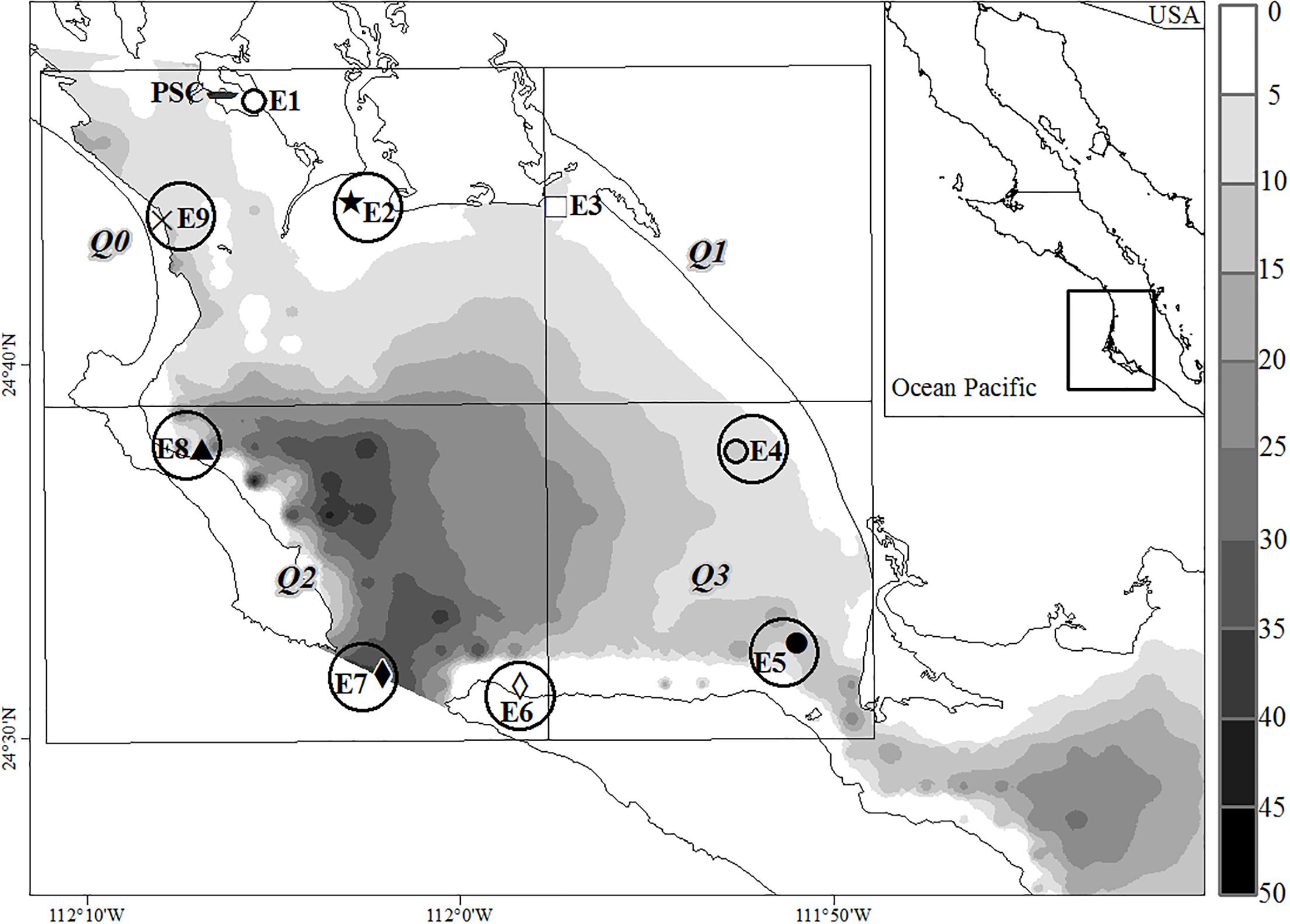
Figure 1. Bahia Magdalena lagoon, Mexico. PSC, San Carlos Port. Sampling sites for hydrological analysis. E1, El muellecito; E2, Punta Gato; E3, La Herradura; E4, La Palmita; E5, Canal La Gaviota; E6, Yellowtail amberjack culture; E7, lagoon’s mouth; E8, Magdalena Town; E9, Oyster culture. Symbols show the sampling stations and circles the stations where plankton hauls were done. The lagoon was divided into four quadrants Q0–Q1 to FLH analysis. Bathymetry is indicated as a gray scale.
The TW, salinity, and density (TSD), concerning changes in the adjacent marine zone were described with data from E7, located at the channel of communication with the ocean (lagoon’s mouth). The temperature anomalies correspond to the difference between the TW measured on the surface and the 1981–1998 average (Lluch-Belda et al., 2000). On the other hand, the dissolved oxygen, percentage of oxygen saturation, nitrite, nitrate, phosphate, and silicate concentrations were calculated as the semester averages per depth-level (0 m, 4–10 m and >15 m) to compare their variability among years. We also contrasted the nutrients concentrations and Chl-a of the inner (E1, E2, and E9) and outer stations (E6 and E7). The comparisons between levels, semesters and stations were made with the non-parametric rank sum test of Mann–Whitney and the Kruskal–Wallis H test (Sokal and Rohlf, 1987).
Monthly values of each sampling station, as well as variables of each year, were analyzed by principal component analysis (PCA) to identify the most influential variables on the system variance, both in spatial and temporal aspects. Average values of each variable per sampling station were subjected to an agglomerative hierarchical cluster analysis (medium link method) to complement this analysis, based on similarities of the Pearson’s coefficient of correlation. Both analyses were done with XLSTAT for MS Excel.
Collection of phytoplankton samples was simultaneous to the sampling for hydrological analysis, except in winter 2016, when there was no biological sampling. Samples were preserved in Lugol’s iodine solution and stored in the dark until analyzed. Enumeration of phytoplankton was done with the Utermöhl method (Hasle, 1978; Andersen and Throndsen, 2004; Reguera et al., 2011). Analysis was done mainly on micro-phytoplankton (20–200 μm); the identification of nanoplankton species (<20 μm) was not possible, due to the usual limitations of the inverted microscope low magnification. We were able to recognize the size, shapes and some morphological characters such as flagella, pigmentation, and aggregations.
Community structure analysis was made to determine changes in the taxonomic composition, cell density, percentage of diatoms and dinoflagellates, and species richness-diversity (Shannon and Weaver, 1949). Analyses were applied to two representative sampling stations E6 and E9. The former is where the marine influence is higher, near the lagoon’s mouth, and the latter within the lagoon. The analyses included between 70 and 80% of the total number of samples collected between January 2015 and August 2017. Other approach consisted in identifying the cell abundance peaks in the seasonal variability, including algal blooms (AB), using 50% of the total samples. In this paper, AB is an event in which cell density was higher than the “normal cycle of phytoplankton biomass” in a region (Smayda, 1997). In our case, it was defined as higher than 5 × 10⁵ cell L-1 based on the average cell density of the spring and fall blooms described by Gárate-Lizárraga and Siqueiros-Beltrones (1998).
The cell density data available from all sampling stations (50% of total samples) were related with Chl-a records of all depth levels and by level by simple regression analysis to test its usefulness as an indicator of phytoplankton abundance. On the other hand, the sampling frequency was once a month, losing the rest of days. Therefore, daily and monthly composite images of the fluorescence of Chl-a (FLH; pixel size 0.125°) collected by MODIS-Aqua satellite (OceanColor- NASA) were used to describe the seasonal variability. FLH was related with cell density (surface) using linear regression. FLH data were recorded on the date of sampling or the nearest one, in case of cloudiness. For this analysis, the lagoon was divided into four quadrants (Figure 1), with sampling stations distributed as follows: upper left quadrant, northwestern zone stations (E1, E2, and E9); upper right quadrant, northeastern station (E3); lower left quadrant, lagoon’s mouth stations (E8, E7, and E6); and lower right quadrant, south and central lagoon stations (E5, E4).
Zooplankton samples were collected with a standard conical net (0.6 m mouth diameter, 505 μm mesh) equipped with a mechanical digital flowmeter (General Oceanics); it was towed horizontally in a semicircular trajectory at 1 m depth approximately at a speed of 1 m s-1 on all stations (Figure 1) except in the E1 and E3 stations. Samples of five stations were fixed and preserved in a 4% formalin solution buffered with a saturated sodium borate solution. A neutral red solution was added approximately 10 min before fixation to stain living animals. Samples of E5 and E9 stations were fixed with alcohol. ZB (mL 100 m-3) was determined by the displacement volume method (Beers, 1976) and mortality as the percentage of zooplankton (%ZD) that did not absorb stain (Elliott and Tang, 2009). Coverage of samples in the case of biomass analysis was 84.8% in E7, 97% in E5 and 100% in the remaining stations. Analysis of %ZD was focused on E6 (sampling coverage 96.9%) and E2 (sampling coverage 87.8%).
The relationship between environmental and biological datasets was analyzed with bivariate and multivariate statistical analysis. The relationship between the ratio of diatoms’ cell abundance (%D) to total diatoms + dinoflagellates, with TW and silicate, was analyzed using a generalized additive model (GAM) with a quasi-binomial type error distribution, using the R package mgcv (Wood, 2006; R Core Team, 2016). FLH values were related to average TW of the water column in each station by simple linear regressions.
A canonical correlation analysis (CCA) was carried out to identify and measure the association among environmental and biological variables, using the R Vegan package (Oksanen et al., 2018). Stations E6 and E9 were the only datasets included. The environmental variables set (X) included UI (average of the five previous days), TW, salinity, ammonia, nitrite, nitrate, phosphate, silicate, Chl-a, oxygen, while the biological (Y) set contained phytoplankton cell density (Cd), diatom cell density (CdDiat), dinoflagellate cell density (CdDino), percentage of diatoms (pDiat), percentage of dinoflagellates (PDino), and ZB. The variables were transformed (log, and ArcSin for percentages) so that the data distribution was symmetrical and standardized to put them on the same scale.
The Cancor (canonical correlation) function in the Vegan package also gives a determination coefficient, R2 and R2 adjusted by the number of data of the biological variables given the environmental ones (Y—X) derived from a redundancy analysis procedure (RDA) and the correspondent values of those indices of the environmental variables given the biological ones (X—Y).
Results
Temperature Anomalies in the Environment
Air temperature in Ciudad Constitucion from 2008 to 2013 was like the 1961–2002 average (Ruíz-Corral et al., 2006), so anomalies ranged from -1 to 1°C, except for 2010, which were lower than -1 due to La Niña. In contrast, anomalies ranged mostly between 1 and 4°C from 2014 to 2017. The warmest periods were recorded in winter and fall of both years 2016 and 2017. Anomalies were more noticeable in the fall of 2017 than in the rest of the period.
Upwelling Phenology
The 1967–2010 average CUI positive slope (Figure 2A) showed that conditions are favorable for upwelling throughout the year, whereas the slope changes suggest that there are four upwelling seasons (US). Upwellings are more frequent and stronger in spring (US-spring) and fall (US-fall) when the slopes are steeper. US-spring covers from the first days of March to the last week of June, when the NW winds predominate. On average, there are 55 days when UI > 100 and these are more frequent since March. There are few days in which UI > 100 (average 9). During winter (January and February) and summer US (July to September), the slopes are smaller, and there are fewer strong events than in the US-fall (September to December).
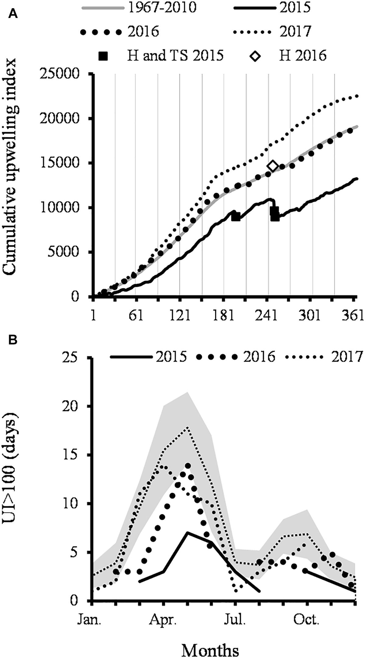
Figure 2. Upwelling phenology. Gray line is 1967–2010 average; H, hurricanes; TS, tropical storm. (A) Cumulative upwelling index of 1967–2010 average and 2015–2017. (B) Days in which the upwelling index was greater 100 m3 s-1 100 m coastline (UI > 100). Gray band shows mean ± SD.
The slopes of the four US in 2015 were lower than the average (P < 0.05), the length of US-spring was shorter (23 March–14 June) and only 18 days had UI > 100 (Figure 2B). Atypically, during the US-summer period, there were two downwelling episodes (Figure 2A), the first one (July 17–18) coincided with the Tropical Storm (TS) Dolores and the second (7–10 Sept) with the dissipation of TS Kevin and the category-2 Saffir Simpson Hurricane (H) Linda.
The CUI profile of 2016 was like the average, although the US-spring ended almost 2 weeks before than average date, there were fewer strong events (31) (Figure 2B) and these began until the last week of April; on the other hand, there were more strong events than usual only in November. In 2017, the slopes of the four US were higher, and during the US-spring there were 55 days in which the UI > 100, and some of them occurred in the first days of June. These events were stronger than the average, in variable percentages between 5 and 10%.
Variation of Temperature, Salinity, Density, and Dissolved Oxygen in the Water Column
The data show that changes of TW throughout the year occur in two periods: temperate and warm, associated with mixing and stratification processes, respectively. The temperate period covers from December–January to June–July, and the coldest months are April–May when upwellings are stronger. The warm period is from July–August to November–December, and the highest TW occur in August–September.
TW and the length of temperate and warm periods varied widely among the 3 years (Table 1 and Figure 3A). The temperate period was shorter in 2015 and 2017 than in 2016, when it lasted until July despite coinciding with the end of the El Niño. The lowest TW was recorded in 2017 at the bottom level and coincided with strong upwellings. In contrast, during the warm period of 2015, TW was high and uniform along water column while a thermocline was formed in the other 2 years; also, the warmest month was August, instead of September as usual. On the other hand, TW was higher in the warm period of 2017 than in 2016.
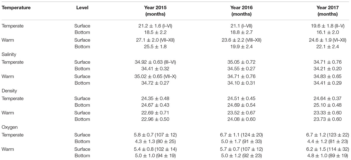
Table 1. Average values and standard deviation of temperature (°C), salinity, density (kg l-1), and dissolved oxygen (ml l-1 and saturation value %) per season of the year and depth level.
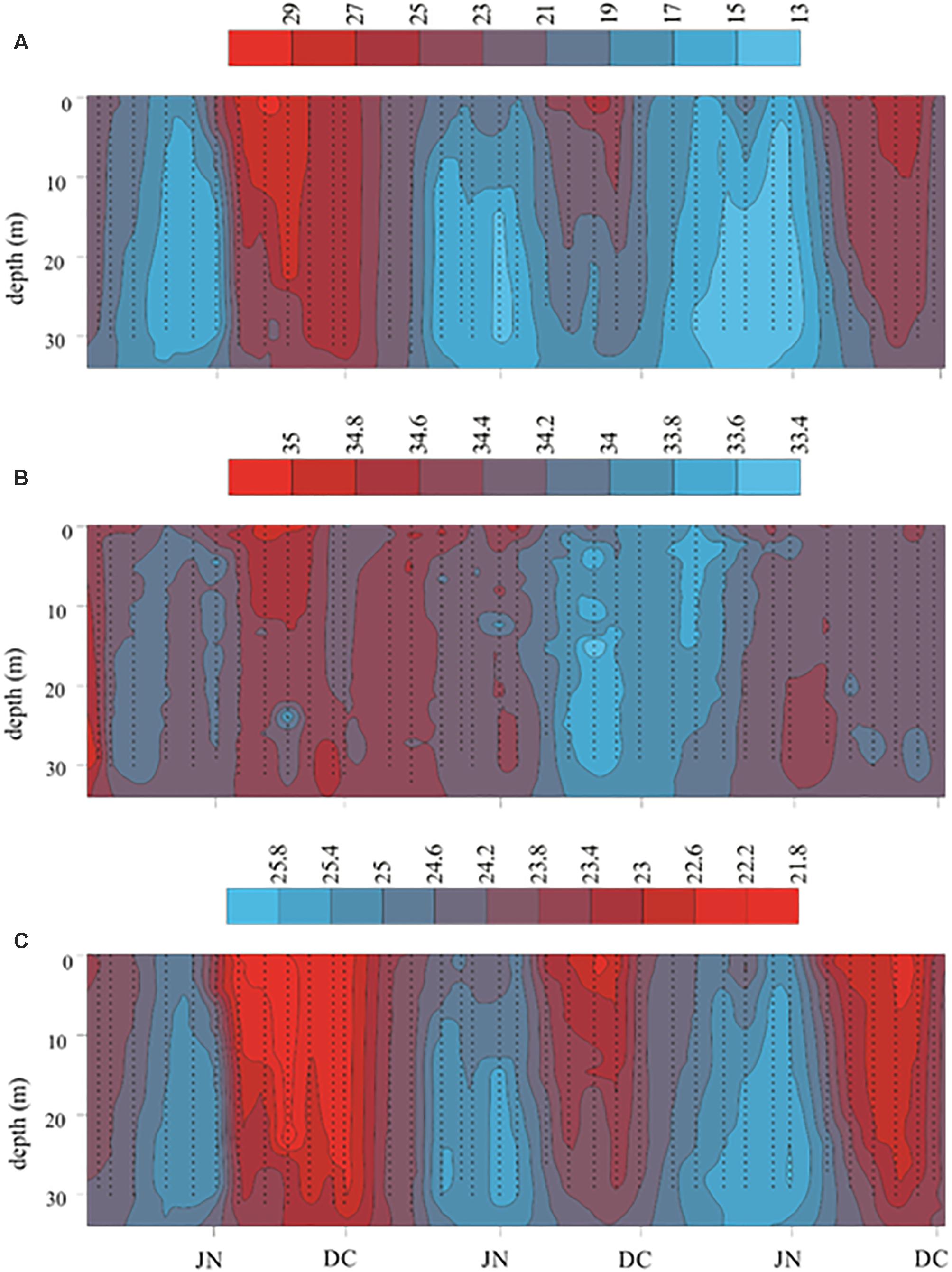
Figure 3. Temperature (°C), salinity and density (kg m-3) monthly distribution in the mouth of Bahia Magdalena from 2015 to 2017. (A) Temperature; (B) Salinity; (C) Density. JN, June; DC, December.
The temperature anomalies in 2015 were positive most of the year, but values higher than +3°C were recorded from June to December at stations E6, E7, and E8, near the lagoon’s mouth. The highest anomaly (+5.8°C) was recorded at station E7 in July, due to the warm water input from the ocean and it coincided with the beginning of the El Niño and the longest southward extension of TB. The 2016 anomalies were positive in winter and normal-positive in spring, when the El Niño was decaying; negative in summer and positive in fall although a moderate La Niña began. The greatest anomalies were measured in the stations E1 and E9, inside the lagoon as usual, but they were very high (+2 to +5.03°C). Anomalies varied between just under -2°C and +3.78°C in 2017; negative anomalies were recorded in winter and spring in almost all stations and in September, while high positive anomalies were recorded in April and August in the inner station (E1), as well as in October and November at the lagoon’s mouth (E7).
Salinity was more variable than temperature throughout the year. On average, the highest values were measured at the surface and the lowest at the bottom (Table 1). In the 2015, salinity was lower during the first semester than in the second one, while the lowest values were recorded from March to June and the highest from July to October. In 2016, the average salinity from January to August was like that of the second semester of 2015, while the lowest values of the 3 years were observed during the rest of that year (Table 1 and Figure 3B). In the first semester of 2017, salinity was like that of the previous semester, while in the second semester it increased both in the area and in depth.
Density (TSD) increased from the surface to the bottom and, in general, the values of the first semester were higher than those of the second. On the other hand, TSD was lower along 2015 than in the other 2 years, while the highest values of the temperate season were recorded in 2017, and those of the warm one in 2016 (Figure 3C).
Oxygen concentration (mL L-1) and the percentage of saturation (%) were higher on the surface and decreased toward the bottom during the 3 years (P < 0.05; Table 1). Both variables were lower in 2015 than in 2016 and 2017 (P < 0.05). The percentages of saturation in the January–June 2015 semester were lower in 14% (2016) and 13% (2017), respectively; however, the differences in the same period at mid-depth (4–10 m) and near the bottom (>15 m) were less evident (Table 1). In the July–December semester the saturation percentages in the first 10 m also were lower in 2015 than in 2016 and 2017; however, this pattern was inversed with 2 and 5% more saturated in 2015 concerning 2016 and 2017 in stations deeper than 15 m.
Variation of Nutrients and Chlorophyll-a in the Water Column
Nitrate, phosphate, and silicate concentrations were higher during the first semester of each year than in the second one (P < 0.05) and increased from the surface to bottom along the water column (P < 0.05). In general, the concentration of nitrate and phosphate was low during 2015, increased in 2016, and reached to maximum values during 2017 (Figures 4A–D), while the silicate was more variable (Figures 4E,F). On average, nitrate, phosphate and silicate content was higher at the stations near lagoon’s mouth (P < 0.05; Figures 5A–F), but phosphate and silicate concentrations were higher in the interior of the lagoon in 2015. The ammonium concentration was relatively more abundant in the inner stations in 2015 (P = 0.07) and during the first semester of 2016 at mid-depth (P = 0.001; Figures 4, 5G,H).
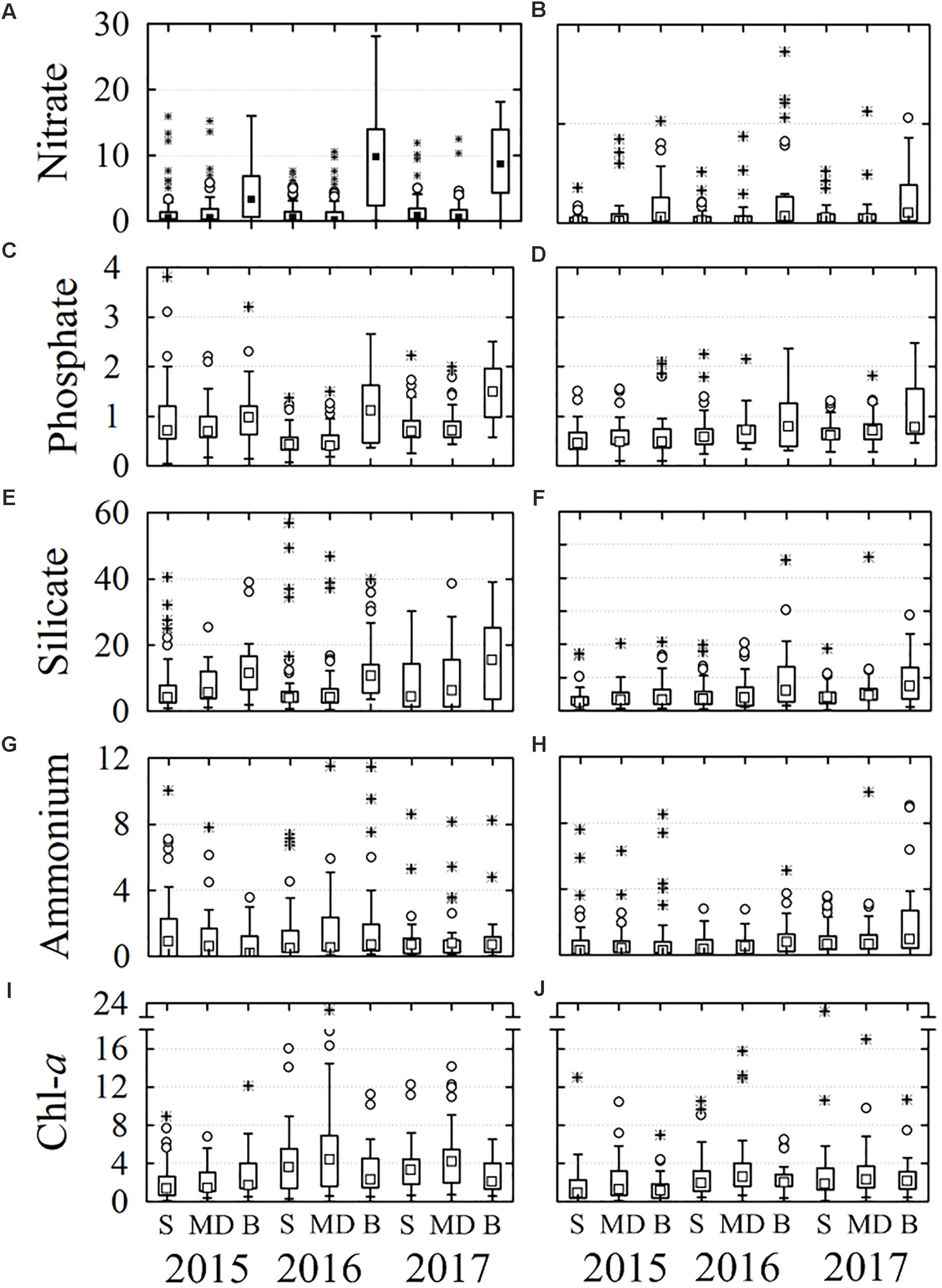
Figure 4. Box and whiskers graphs of nutrients and chlorophyll-a, recorded from 2015 to 2017. Boxes include percentiles 25th, 50th, and 75th; ○ outliers, ∗ extreme values. The panels (A,C,E,G,I) correspond to the first semester and (B,D,F,H,J) to the second one of each year. S, surface; MD, mid depth; B, bottom.
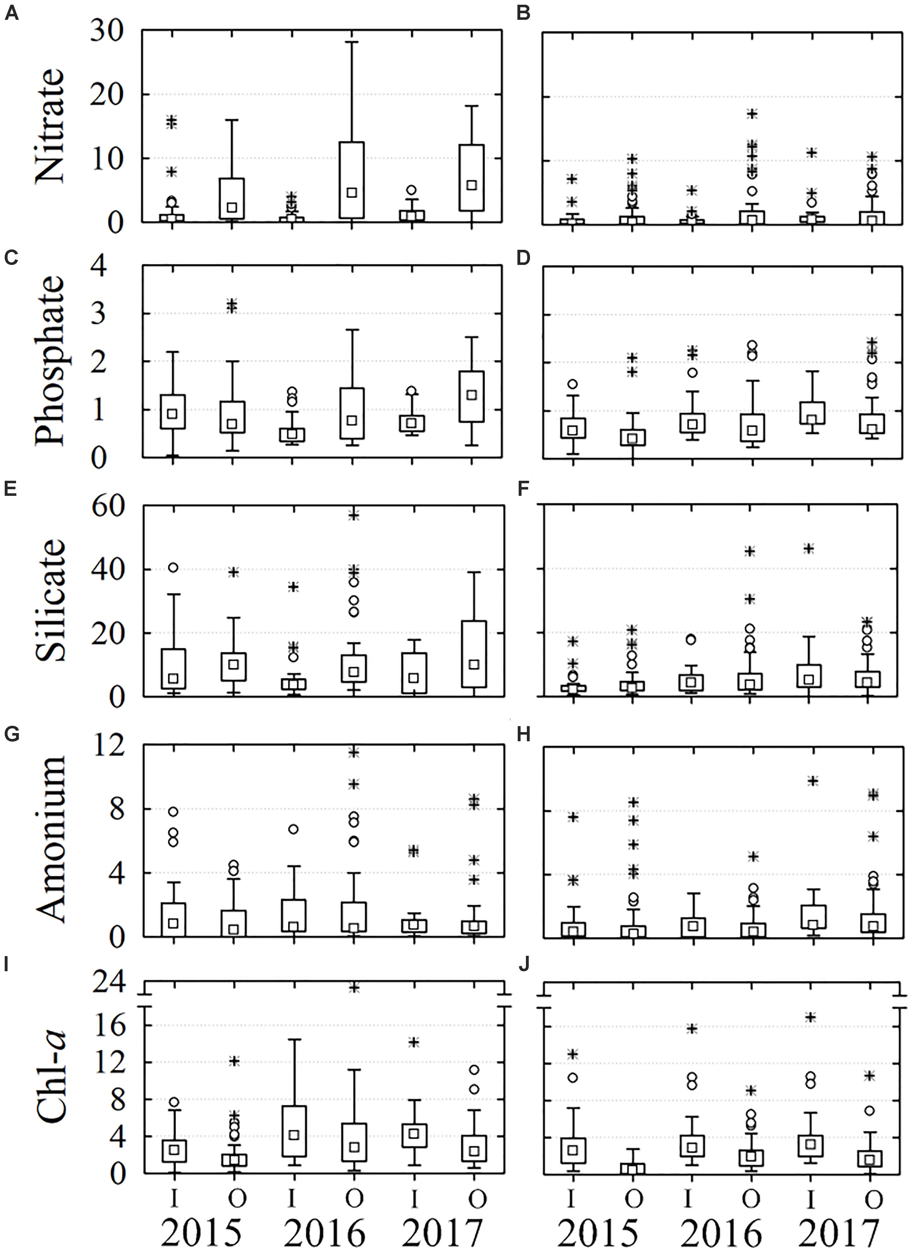
Figure 5. Box and whiskers graphs of nutrients and chlorophyll-a, recorded in the inner (I) and outer (O) stations. Boxes include percentiles 25th, 50th, and 75th; ○ outliers, ∗ extreme values. The panels (A,C,E,G,I) correspond to the first semester and (B,D,F,H,J) to the second one of each year. Inner stations: 1, 2, 9; outer stations: 6, 7.
The nitrate, phosphate, and silicate concentrations were similar at surface and mid-depth levels and greater at the bottom during the first semester of the 3 years (Figures 4A,C,E). On average nitrate concentration at surface and mid-depth levels was <3 μM and it doubled at the bottom (>8 μM), whereas phosphate content was from <1.0 μM to 1.0–1.6 μM at the bottom. The silicate concentration was very high in comparison with the other nutrients (Figures 4E,F), but the difference between the concentrations of the surface-mid-depth (≤10 μM) and the bottom was proportionally lower (13–16 μM); on the other hand, the highest concentration of silicate was recorded during the first semester 2017 (Figure 4E). In the second semester of each year, the nutrient concentrations were lower than in the first semester, but the trend among years and from the surface to bottom was like that of the first semester (Figures 4B,D,F).
Nitrite concentration was lower than other nutrients in the water column (<1 μM) during the study period, but it was slightly higher in 2017 (1.5 μM). Ammonium content tended to be higher in the deeper layer, except in the first semester 2015 when high values were recorded in surface and the inner stations and 2016 at mid-depth (Figures 4G, 5G). The concentrations during the second semester were higher in the inner stations, but there were no significant differences with outer stations (Figure 5H).
Chl-a content was higher in the first semester than in the second one (P = 0.02) as happened with nutrients. The distribution along the water column (Figures 4I,J) differed because, on average Chl-a was more abundant at mid-depth, except in 2015 when it was at the bottom (P = 0.004). Chl-a concentration was lower in 2015 than in the other 2 years (P < 0.05). The highest average values were recorded during the first semester 2016 at mid-depth (5.2 mg m-3 Figure 4I). On the other hand, Chl-a was more abundant in the inner stations than in the outer (P < 0.01), located near the lagoon’s mouth, but the differences were more evident in 2015 due to the concentrations were proportionally lower in the outer stations than in 2016 and 2017 (Figures 5I,J).
The first PCA component (PC1) explained 25% of the variance in 2015, while in 2016 and 2017 it explained 43 and 47%, respectively. The second component (PC2) explained just fewer than 20% in the 3 years. Variables having the highest correlation with PC1 were TW (negative sign), as well as nitrate, phosphate, and silicate (positive sign), located at opposite ends of the horizontal axis in the PCA plot (Figure 6). However, the correlation of PC1 with TW, phosphate, and silicate in 2015 was lower than in the other 2 years, whereas that of nitrate was high during the whole period. The correlation of oxygen with PC1 increased in 2016 and 2017 (Figures 6B,C).
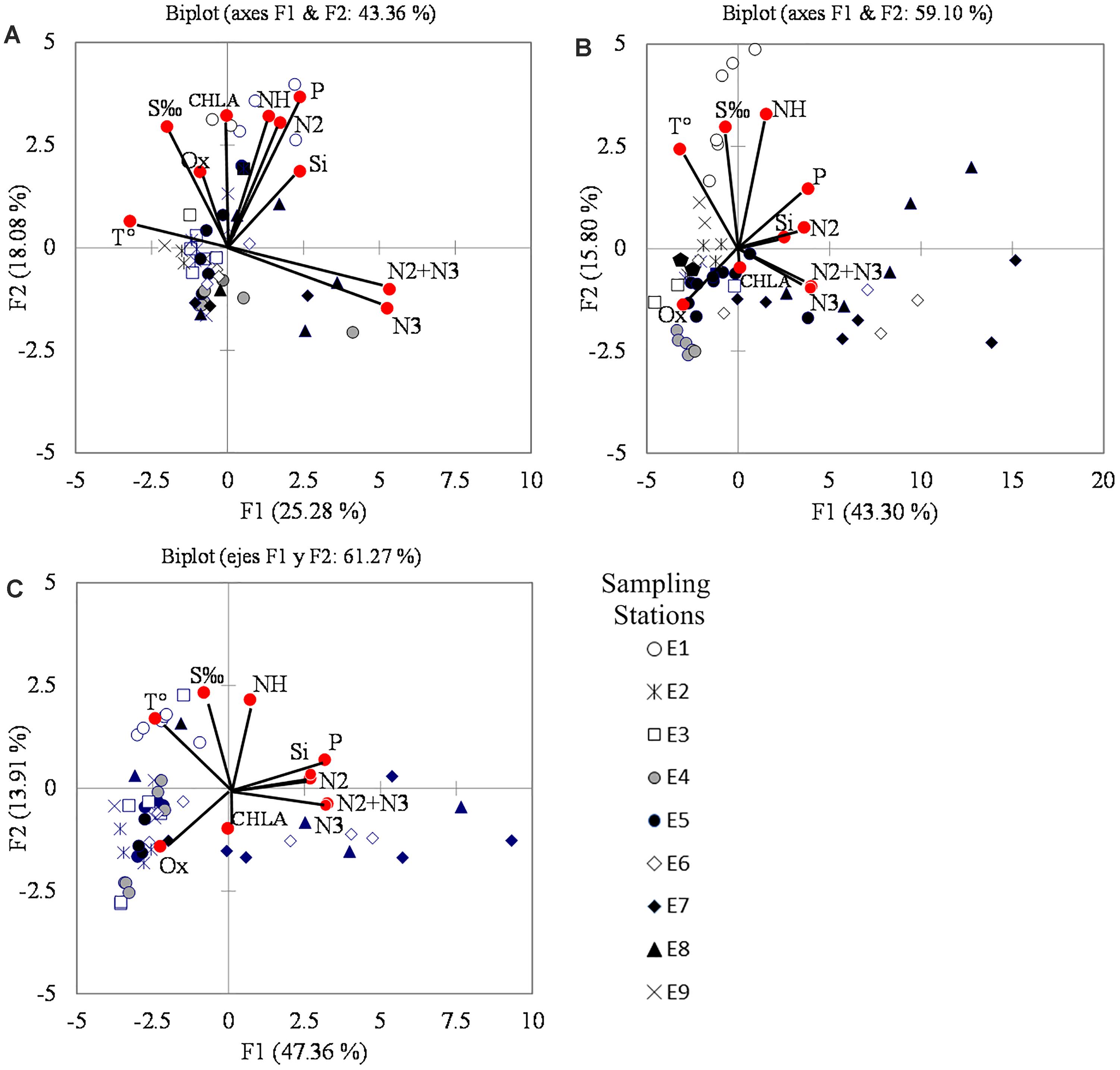
Figure 6. Principal components analysis (PCA) ordination biplots, and location of the sampling sites. (A) 2015; (B) 2016; (C) 2017. The markers show the sampling stations according to Figure 1. Variables key: T°, temperature; S‰, salinity; Ox, oxygen; N3, nitrate; N2, nitrite; NH, ammonium; P, phosphate; Si, silicate; CHLA, chlorophyll-a.
The most important variables on the PC2 were salinity, ammonium, and Chl-a (Figure 6). The position of Chl-a was on the positive segment of the vertical axis, near phosphate, ammonium, and silicate in 2015; while it was in the negative segment, close to nitrate, in 2016 and 2017 (Figures 6B,C). Oxygen was important in this component, and it was found in the upper left quadrant in 2015, but moved to the lower left quadrant in the other 2 years, when its importance increased in PC1.
The position of the sampling stations in the PCA plot changed among quadrants throughout the year, so when nutrient concentrations were high, they were found in the positive segment of the horizontal axis, but when TW increased they moved toward the left quadrants. On the other hand, when nutrient concentration (especially ammonium) increased, there was a positive displacement along the vertical axis. The opposite occurred when nutrient concentration decreased, but the extent of the change was comparatively less than that observed on the horizontal axis. In 2015, the influence of ammonium was higher than in 2016 and 2017.
The location of the stations in the PCA plot allowed distinguishing the variables with greater influence in each site. Stations closer to the lagoon’s mouth (E6 and E7) tended to appear in the lower quadrant and especially in the lower right, where nitrate and nitrite appeared, while E1, E9, and E5, located at the north and the east in the lagoon (Figure 1), appeared more frequently in the upper quadrants where temperature and salinity had more influence (Figure 6). E3 and E4 appeared in the left lower quadrant which probably means that it was influenced by both marine and terrestrial environments, while E8 was found in the upper and lower quadrants depending on the season of the year, so it was close to nitrate in spring in the 3 years and to the temperature in 2017.
Cluster analysis showed that the similarity between stations was very high. In the 3 years (Figures 7A–C) the stations closest to the lagoon’s mouth (E6, E7, and E8) formed the first group, and those located in the interior the second one, although there were changes among those that presented more association, especially in 2016 and 2017 (Figures 7B,C). In 2015 the E1 station was separated from both clusters (Figure 7A).
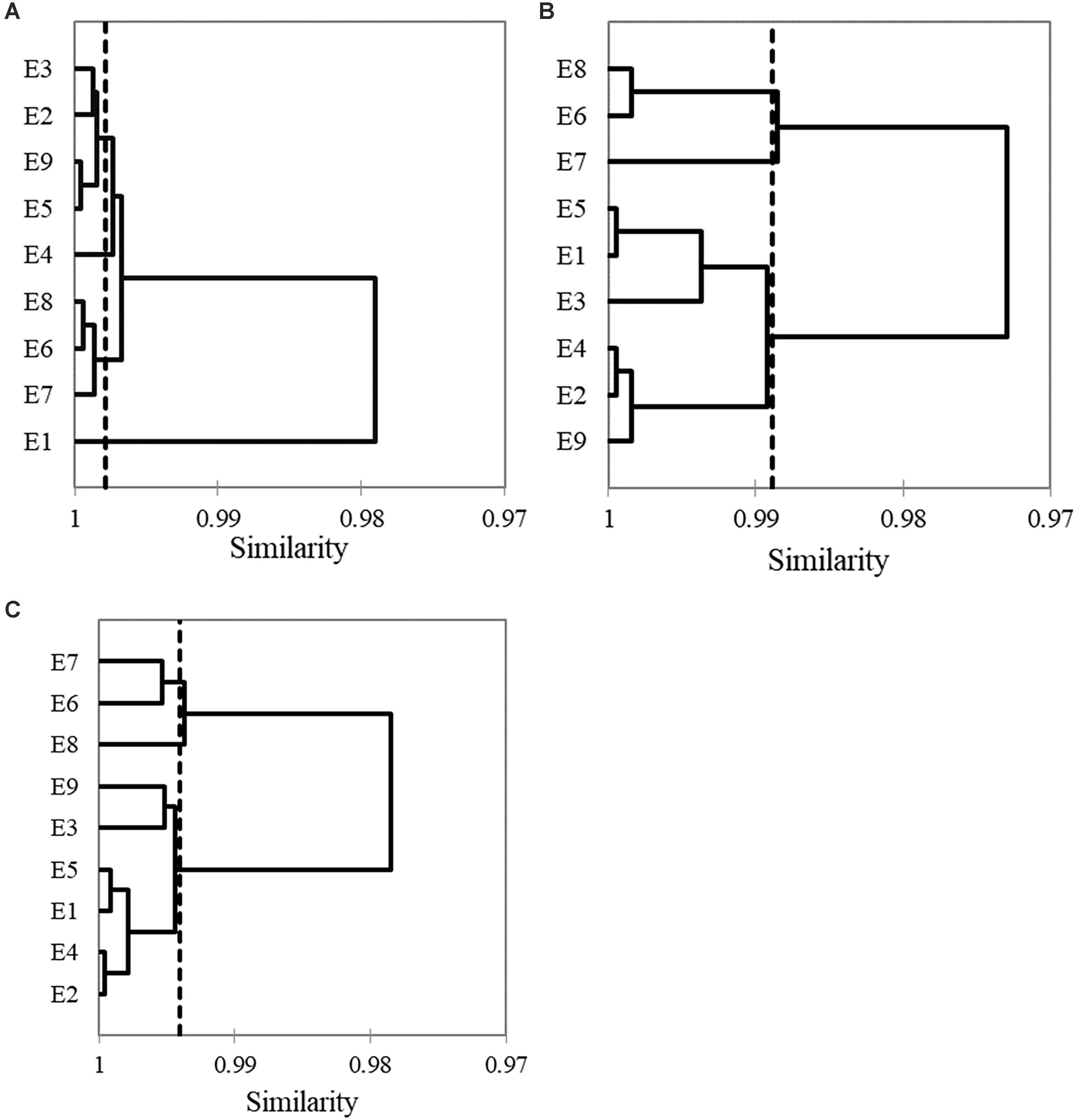
Figure 7. Cluster analysis of hydrological averaged data. (A) 2015; (B) 2016; (C) 2017.
Indicators of the Structure of Phytoplankton Community
Community species composition included members of the taxonomic groups Cyanophyceae, Bacillariophyceae, Dinophyceae, and Dictyochophyceae as well as nanoplankton forms in both stations E6 and E9. In E9 also some species of Euglenophyceae appeared. The classes with higher species richness and cell density were diatoms and dinoflagellates. Different patterns of diatoms and dinoflagellates abundances among the 3 years and between E6 and E9 were found (Figure 8). At the E6 station during 2015, diatoms were dominant in winter and the beginning of the spring, meanwhile during the rest of that year dinoflagellates were the main group along column water (Figures 8A,C,D) except in October, when diatoms were abundant at the bottom. In 2016 there were no winter data. Dinoflagellates were more abundant at surface and mid-depth during spring and the beginning of summer (Figures 8A,C) while diatoms were predominant in fall and at the bottom all year (Figure 8D). In 2017 diatoms were more abundant from January to April and in July while dinoflagellates were more abundant in May (in the three levels) and in June (mid-depth, bottom). The diatoms were the main group at E9 (Figures 8B,E), and only in 2016, there were percentages of dinoflagellates greater than 10%.
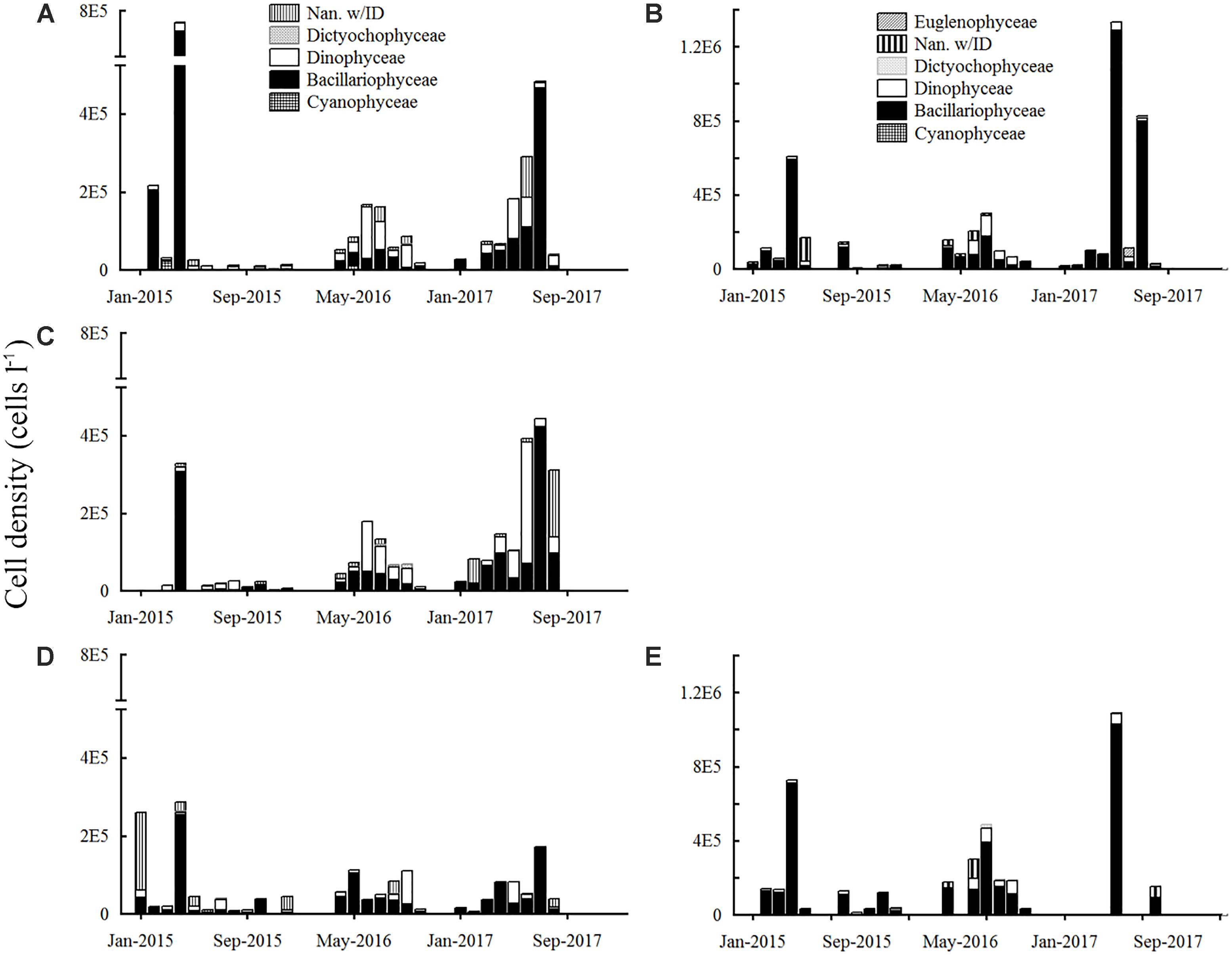
Figure 8. Phytoplankton cell density in the sampling stations E6 (left column) and E9 (right column) (A) E6 surface; (B) E9 surface; (C) E6 mid-depth; (D) E6 bottom; (E) E9 bottom.
The trend of the species composition and cell density was as follow: in 2015, the highest abundance at E6 was recorded in January, February, and April. Nanoplankton was the main component in January at the bottom (≈197 × 103 cells L-1: 76%), and also in May and December but its cell density was lower. Diatoms were the main group from February to April (Figures 8A,C,D). There was an AB in April, and the highest cell density was recorded at the surface (≈767 × 103 cells L-1). The AB was composed of the chain-forming diatoms Eucampia zodiacus (55%), Leptocylindrus danicus (9%) and Chaetoceros curvisetus (8.5%). In the rest of the year, cell density was smaller than 43 × 103 cells L-1, and abounded nanoplankton and dinoflagellates: Prorocentrum balticum, Prorocentrum dentatum, and Prorocentrum spp. were the most abundant species. The cell density at E9 was higher in the bottom and diatoms were the main group (Figure 8E), except in fall (surface; Figure 8B), when phytoplankton was scarce. There was an AB in April (≈728 × 103 cells L-1; bottom), composed mainly of E. zodiacus (49%), C. curvisetus (12%), Chaetoceros cf. radicans (5.8%) and Dactyliosolen phuketensis (5.6%).
Between April and October 2016 (months with available data), in both E6 and E9, the highest density occurred in June and July at mid-depth but at E6 cell density was around 170 × 103 cells L-1, whereas at E9 it was of 200 × 103 and 487 × 103 cells L-1, respectively. At E6, dinoflagellates were the dominant group at the surface and mid-depth from June to September (e.g., Prorocentrum cf. minimum, Tripos furca, Scrippsiella sp.), while the diatoms (Diploneis cf. smithii, Guinardia flaccida) were at the bottom except in September. In E9 the most significant cell densities were recorded in July, and the most abundant species were the diatoms Ditylum brightwellii, Nitzschia sp., and Cylindrotheca closterium. Nanoplankton was abundant in July and August.
In 2017, the cell density increased at E6, from April to June–July, when more than 400 × 103 cells L-1 were accounted (Figures 8A,C,D). In June, the abundance was greater at mid-depths, and the most abundant species were an unidentified dinoflagellate (62%) and the diatom Thalassiosira sp. (14%). In July, the highest values were recorded at the surface and mid-depth, and an AB composed by diatoms in more than 90% occurred. The most abundant species (surface-mid-depths) were the diatoms Rhizosolenia setigera (14–45%), Dactyliosolen fragilissimus (34–12%), Guinardia striata (18–10%), and L. danicus (14–10%). In E9, the most intense blooms of the 3 years were observed in May (>1 × 10⁶ cells L-1) and July (>800 × 103 cells L-1), and they were mainly composed of diatoms (90%; Figures 8B,E). In May, the most abundant species were the diatoms D. fragilissimus (56% surface–50% bottom) and Pseudo-nitzschia spp. (delicatissima complex) (16–12%), while in July Rhizosolenia setigera (50–70%), G. striata (20–0%) and Guinardia flaccida (17–15%) were the most abundant.
Species diversity, measured with the Shannon-Weaver H index, at E6 was higher than 2.5 at the surface and mid-depths samples at the end of spring or early summer in the 3 years (Figure 9A). In contrast, the lowest values (<1.5) were recorded in winter (2015 and 2017) and fall 2015. The species richness in 2015 was very fluctuating and tended to diminish along the year (Figure 9C), but the highest value (55 species) coincided with the April AB. In 2016 coincided the trend of both H and species richness. In contrast, species richness increased from January to August in 2017, but the highest value was recorded at the surface in July (59). At E9 the lowest diversity was detected in April 2015 and in June 2017, when the most intense blooms occurred (Figure 9B); in contrast, H was greater than 3 at the end of 2015, while the species richness was very similar in the surface and bottom samples (Figure 9D).
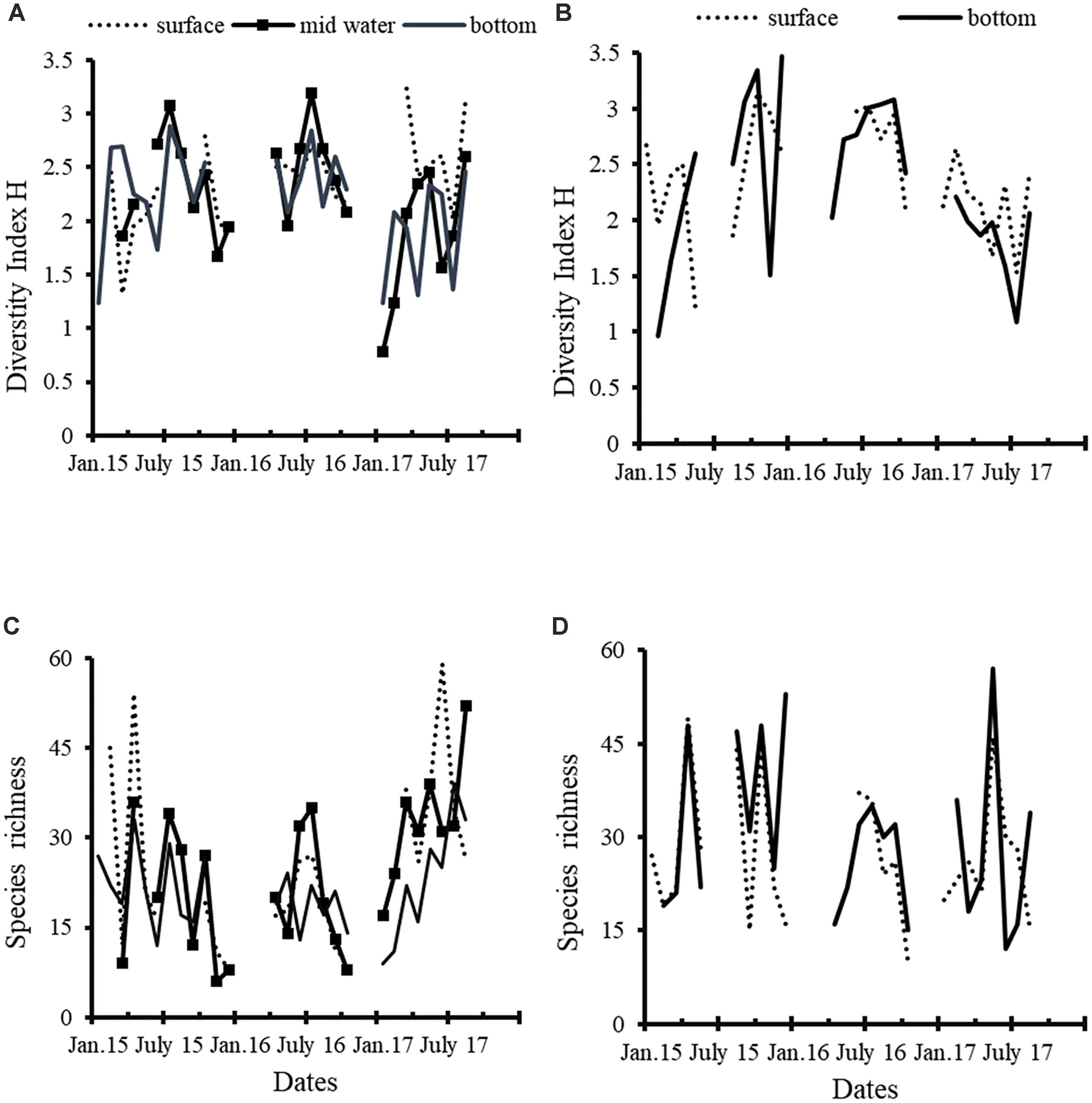
Figure 9. Diversity index (Shannon-Weaver) and species richness in sampling stations E6 (left column) and E9 (right column). (A) E6 diversity index; (B) E9 diversity index; (C) E6 species richness; (D) E9 species richness.
Algal Blooms
Diatoms usually formed the ABs in the 3 years, but in June 2017 it was recorded an AB of an unidentified nanoplankton dinoflagellate (Table 2). On the other hand, in 2015 only one AB (April) occurred, in 2016 two (July and September), and several in 2017 (April–July).
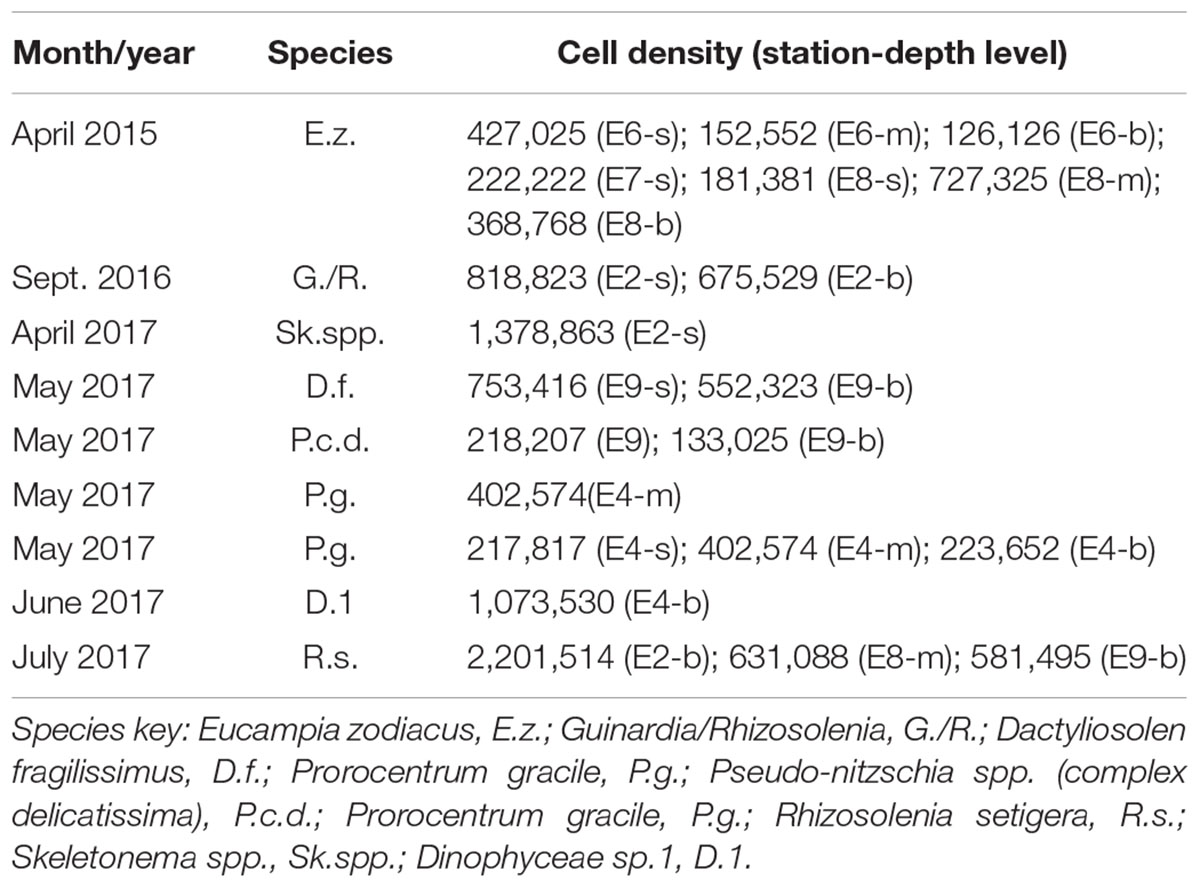
Table 2. Algal bloom recorded on April 2015, and several months of 2016 and 2017 in the surface (s), mid-depth (m), and bottom (b) by sampling station and depth level.
In 2015, as already described, there was an AB of E. zodiacus in April. This species was distributed throughout the lagoon, although it was more abundant in stations with greater marine influence (E6–E8, Table 2) and FLH images suggested that the AB was introduced from the Pacific Ocean. In 2016, the cell density of the AB of July was much lower than in 2015 (≈500 × 103 cells L-1) and covered the entire lagoon, although the highest densities were observed at E9 (D. brightwellii and Nitzschia sp.) and E8 (Pseudo-nitzschia cf. delicatissima). In the rest of stations, the most abundant species was D. brightwellii. The AB of September was recorded at E2 (>675 × 103 cells L-1), and it was composed mainly by Guinardia/Rhizosolenia. FLH images showed that this AB was confined in the north of the lagoon. In 2017, there were blooms from April to July, mainly formed by the diatoms Skeletonema spp. (April), D. fragilissimus (May), Pseudo-nitzschia spp. (delicatissima complex) (May), and the thecate dinoflagellate Prorocentrum gracile (May), an unidentified nanoplankton dinoflagellate (June) and R. setigera (July). The highest cell density was recorded in July in the interior of the lagoon (Table 2).
Indicators of Phytoplankton Density
The relationship between cell density with Chl-a and FLH was positive and significant (P < 0.05) with cell densities lower than 200 × 103 (E6) and 600 × 103 cells L-1 (E9). When they exceeded these values, both Chl-a and FLH were very variable. The percentage of explained variance of Chl-a by the cell density at the three levels was 38% (E6) and 47% (E9), while the percentage obtained from the regression between cell densities measured at the surface and FLH was 65.9% (E6) and 27% (E9), respectively. The above allowed inferring that FLH variations described the trend of cell density near the lagoon’s mouth, and Chl-a in the interior of BM.
Variations in FLH (monthly composite images) suggested that the seasonal pattern of the cell density was similar in the 3 years although magnitude differences. The values were maxima in April–May (2015), May (2016), and July (2017), and FLH was higher in the inner stations E2 and E9 (Figure 10A) than in the outer E6 and E7 (Figure 10B). The length of the period in which FLH was high and also cell density, extended from 3 (2015) to 6 months (2017).
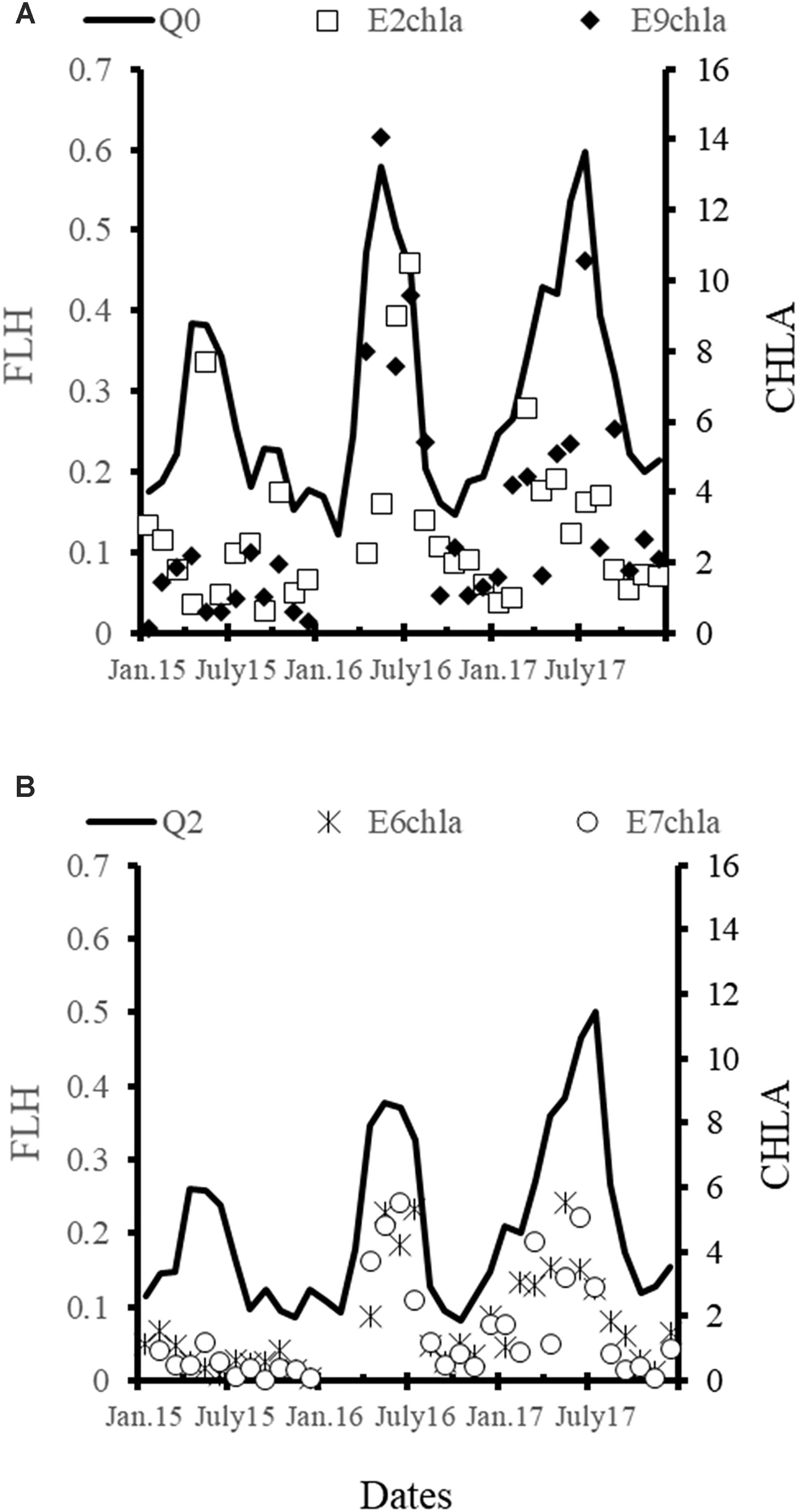
Figure 10. Time series of the chlorophyll-a measured (mg m-3) in situ and the fluorescence of the chlorophyll-a (mW cm-2 μm-1 sr-1) recorded by MODIS-Aqua satellite. (A) Quadrant 0 and chlorophyll data of E2 and E9; (B) Quadrant 2 and chlorophyll-a data of E6 and E7.
Zooplankton Biomass
The zooplankton biomass average (ZB) was relatively high from January to August of 2015 (>60 mL 100 m-3), and after that month followed a decreasing trend that continued until December 2017 (<35 mL 100 m-3) (Figure 11A). During 2015, high ZB values occurred from January to April, and again in July–August. The high values of the first semester were recorded in stations close to, or at the lagoon’s mouth (E7–E8; >100 mL 100 m-3), including the highest (>300 mL 100 m-3), registered in April and June 2015. However, ZB was lower at station E6 also situated near the lagoon’s mouth, where there is a cage fish farming of yellowtail amberjack (Seriola lalandi). At the stations of the interior (E2, E4) and south (E5), there were also high ZB values (>100 mL 100 m-3) during the first semester of 2015 (Figure 11B).
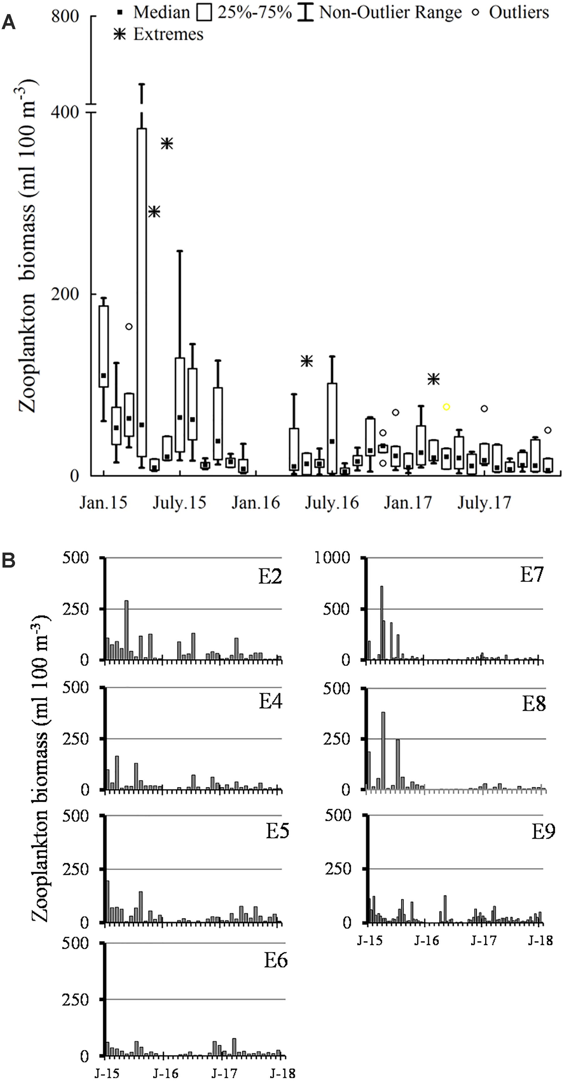
Figure 11. Zooplankton biomass (mL 100 m-3) recorded from 2015 to 2017. (A) Time-series of all data; (B) ZB measured in the E2–E9 sampling stations. J, January.
In 2016, winter months were not sampled. In this year, average abundance decreased year around (<35 mL 100 m-3), with a slight increment in July (Figure 11A). Spatial distribution of the ZB was homogeneous along the lagoon, with some increments (<100 mL 100 m-3) in the inner stations in April (E2), May (E9) and July (E2, E4, E9) (Figure 11B).
The average ZB remained scarce in 2017 as well as in 2016 (<35 mL 100 m-3) (Figure 11A), but no increases were observed in May or June–July, as occurred in the two previous years. That year there were small increments in March–April inside de lagoon (E2, E5, E9), which suggested changes in the zooplankton phenology. The ZB abundance was more variable at the stations located in the northern area (E2) and at the communication channel with the adjacent Bahia Almejas lagoon (E5) (Figure 11B). The ZB at E7 was very low.
Mortality of Zooplankton
The annual average %ZD was 9% and 17% (E6 and E2, respectively) in 2015, and increased in 2016, but while the value almost doubled at E2 (33%) in the interior, the increase was lower close to the lagoon’s mouth (15%). On average %ZD increased slightly at E6 but decreased at E2 in 2017, after February. There is an inter-annual variation of more than 10% of %ZD, and it becomes lower (<5%) in 2017, probably due to the restoration of the primary production cycle given the conditions of availability of nutrients and the blooming of phytoplankton found.
Monthly zooplankton mortality (%ZD) ranged from 5 to 95% at E2 station from 2015 to 2017 (Figure 12A), with two maxima, one in August 2016, when almost 100% of organisms were dead, and another in March 2017 (71%). In comparison, %ZD was relatively lower, in a range of 0–25% in the lagoon’s mouth (E2; Figure 12B), with a maximum in June 2016 (41%). %ZD, in general, was high in concentrations of diatoms and dinoflagellates of less than 50 × 103 cells L-1 and 30 × 103 cells L-1, respectively.
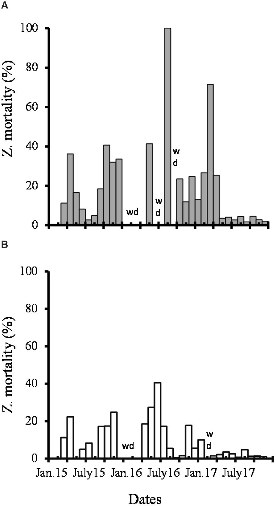
Figure 12. Percentage of dead zooplankton recorded from 2015 to 2017. WD, without data. (A) E2; (B) E6.
Mortality did not show a seasonal pattern in both locations and its fluctuations along the 3 years were as follows: %ZD in 2015 increased in winter, early spring and fall, and decreased in summer. On the contrary, %ZD increased in both sites in spring and declined in fall in 2016. However, %ZD was generally low throughout the year 2017, but with a substantial increase in early spring (Figures 12A,B).
Biological Responses to Environmental Conditions
The relationship between TW and FLH was significant and negative (P < 0.05). The coefficients of determination were larger with data of E6 (R2 = 0.56), E7 (R2 = 0.61), and E8 (R2 = 0.57) than with those of the inner stations (27–30%). In contrast, results were not significant in the E1, located near the port of San Carlos.
The analysis using GAMs showed that the %D was significantly correlated to TW (P < 0.05, deviance explained = 50.7%). However, while %D decreased with increasing temperature in 2015 and 2016, the opposite occurred in 2017, which suggests that other variables, likely nutrients advected from the marine zone during upwellings by tide currents enhanced the diatoms abundance. The GAM applied to %D, and silicate showed a significant relationship (P < 0.05, deviance explained = 66.6%), but 2015 data had a bigger dispersion than those from 2016 and 2017. In these 2 years, the graph was a parabola with low %D at the extremes of the horizontal axis (silicate concentration); in contrast, the diagram of 2015 was very different as data were scattered and did not show any evident trend.
The Pillai’s trace (V = 2.416) resulting from the CCA was significant (0.018 from F-distribution and 0.007 based on permutations), indicating a significant correlation between environmental and biological variables dataset considered in the test. The canonical correlations were high on the first two canonical axes: 0.91 for axis 1 and 0.85 for axis 2. R2 and adjusted R2 of the biological variables given the environmental ones (Y| X) were 0.53 and 0.30, respectively. The corresponding values for the environmental variables given the biological ones (X| Y) were 0.33 and 0.15, respectively.
The CCA biplots (Figures 13A,B) showed that nitrate, phosphate, and silicate were highly correlated with the vertical canonical axis, as did logarithm of cell density (of all species, diatoms, and dinoflagellates). TW showed a high negative correlation on the vertical canonical axis. Diatoms cell density and percentage of diatoms were on opposite sides of the biplot from the dinoflagellates cell density on the horizontal canonical axis. The logarithm of ZB was found in opposite sides of the plot on the vertical axis from the phytoplankton-related variables, although with a low correlation on both canonical axes. In contrast, correlation of UI with both axes was low probably because it is the result of a modeling process of synoptic-scale measured variables. Possible nonlinear relationships masked by the assumptions of this method could be another cause for the low correlation found.
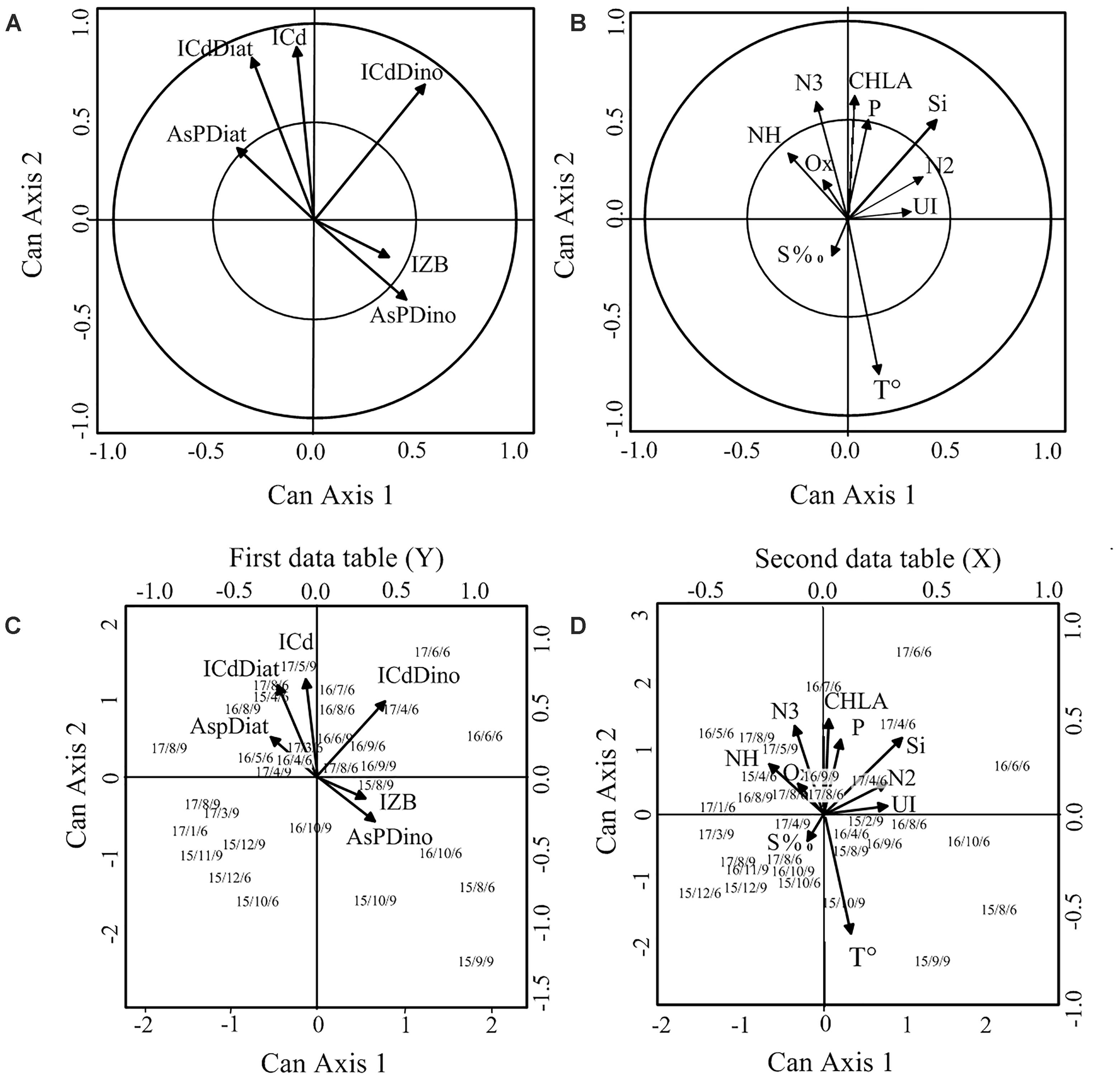
Figure 13. Canonical correlation analysis procedure biplots. (A) Biological variables; (B) environmental variables; (C) position of sampling stations included in the analysis and the biological variables; (D) position of sampling stations included in the analysis and the environmental variables. ICd, log cell density total; lCdDiato, log diatoms cell density; lCdDino, log dinoflagellates cell density; AsPDiat, arcsine of the percentage of diatoms; AsPD, arcsine of the percentage of diatoms. (C,D) Characters chain mean year/month/station number.
In summary, the more noticeable relationships were: the phytoplankton cell density was inversely related with TW and directly related with nutrients while the dinoflagellates percentage (but not the abundance) was directly associated with TW. ZB was inversely related with diatoms and dinoflagellates. %D was inversely related with silicate, and the correlation coefficient showed that it was the most important nutrient.
The position on the plot of sampling dates for the two stations included in this analysis showed a clear pattern according to the timing of samples and the geographical location of the sampling stations. The spring–summer month’s samples appeared in the upper right quadrant with cell densities (total and diatoms) and %D, whereas fall and winter months were more frequent in the lower quadrants with ZB and the dinoflagellate proportion (Figure 13C). On the other hand, samples from April to May, the coldest months, tended to be in the upper half of the plot while August–September, the warmest period of the year, in the lower half (Figure 13D). The position of the samples on the plot along the year changed in a clockwise manner, between those extreme conditions. Station E6 samples tended to be more frequent in the upper right of the plot than station E9 samples taken on the same date. Samplings from 2015 tended to be concentrated toward the lower left quadrant of the plot which is related with warmer conditions, while in 2016 and 2017, are more dispersed and toward the upper right quadrant suggesting a greater influence of marine conditions.
The patterns of the environmental variables in the CCA and PCA plots were consistent between each other, and both were associated with time and spatial factors. Results of the GAM also were consistent with this analysis. In summary, these results showed clear patterns and significant relationships between biological and environmental variables.
Discussion
Local Impact of Global Phenomena
The northeastern Pacific Ocean was very warm from 2013 to 2016 (Leising et al., 2015; Jacox et al., 2016; Zaba and Rudnick, 2016) due to the succession and overlapping of TB and the El Niño. On the other hand, 2015, 2016, and 2017 had been confirmed as the three warmest years on record, whereas 2016 had the global record, 2017 was the warmest year without an El Niño (World Meteorological Organization, Press release 18 January 2018). These global-scale events altered both atmospheric and ocean circulation, which led to the relaxing of the North Pacific Subtropical Gyre, the weakening of the California Current and the limiting of nutrients advection from the North Pacific to Baja California (Mcclatchie et al., 2016; Gómez-Ocampo, 2017).
The characteristics of the temperate and warm seasons in BM changed along the 3 years. In 2015, the temperate season was milder and the temperature in winter and fall was even higher than in the 1982–1983 and 1997–1998 events (Lluch-Belda et al., 2000), probably due to The Blob influence at the early year off Baja California, and the characteristics of the 2015–2016 El Niño which was a combination of Central Pacific ENSO (CP-ENSO) and Eastern Pacific ENSO (Paek et al., 2017). The CP-ENSO results from the southwestward spreading of subtropical atmospheric fluctuations and one of its characteristics is the induction of positive temperature anomalies off Baja California during the winter previous to develop of the El Niño.
In 2016 when the El Niño was decaying, the temperate period was shorter and the characteristics of the warm season were closer to normal than in 2015 and 2017. However, anomalies continued being positive even though La Niña had begun, probably due to high temperatures prevailing at local and global-scale in both, the sea and the atmosphere, as it was evident in Ciudad Constitucion data and from WMO information. A particular phenomenon can change local conditions, as occurred in September when anomalies were negative. Likely because the sampling campaign was carried out on day 8, 2 days after passing of hurricane Newton (Berg, 2017) which decreased temperature due to wind and rain, as well as the advection of cold subsurface water to lagoon since UI increased from 123 to 282 m3 s-1 per 100 m of coastline between the September 3rd and 6th.
Temperature anomalies were negative in the spring 2017, probably due to strong northwestern winds and intense upwellings. In contrast, the conditions were warm at the lagoon’s mouth during the fall, as it happened along Baja California and the west coast of the United States during the warmest year without the El Niño and even though a weak La Niña was beginning at the equator (NOAA, 2017). In 2017, the atmospheric temperature anomalies were very high, and the atmosphere-ocean interaction allowed transference of heat, probably causing positive temperature anomalies in the lagoon.
Upwelling and Nutrient Advection
Coastal upwellings were weaker in 2014 in front of BM (Jiménez-Quiroz, unpublished data) probably due to the combination of high air temperatures, weak winds and a deeper thermocline as happened in the Southern California Current System and the northern and central Baja California under 2014 TB (Zaba and Rudnick, 2016; Gómez-Ocampo, 2017) and other the El Niño (Zaytsev et al., 2003). Warming of the Baja California coast from May 2014 to April 2015 was associated with weak coastal winds unrelated with the El Niño (Robinson, 2016) but coincident with TB. The co-occurrence of TB and the El Niño exacerbated these conditions in 2015, weakened even more the upwellings and shorten the US-spring in front of BM.
The El Niño has been associated with a strong and southeastward displacement of the wintertime Aleutian Low, a weak North Pacific High and a regional pattern of poleward coastal wind anomalies (Jacox et al., 2016), modifying upwelling phenology along California coast (Mcclatchie et al., 2016). IMECOCAL cruise data of central and southern lines (23° and 28°N) during the 2015–2016 El Niño, indicated that the high positive temperature anomalies and the deepening of thermocline and nutriclines led to the interruption of upwellings near coast (Gómez-Ocampo, 2017), in a similar way to our observations in BM.
The comparison of our values with the average of the 2005–2011 time series which comprises ENSO-neutral, La Niña and weak ENSO years, showed that nitrate and phosphate concentrations diminished almost 50% in 2015 (Cervantes-Duarte et al., 2013). When the El Niño ended in 2016, and there were still few strong events, both nitrate and phosphate content increased at the bottom, which together with changes in TW, salinity and density can indicate the nutrient source recovery to the system. At this period began La Niña and probably contributed to strengthen upwellings during fall.
In the first semester of 2017, when the weak La Niña was declining, the characteristics of the US-spring were normal (length and number of strong events), but the upwellings were very strong, diminishing TW and increasing the nitrate and phosphate concentrations significantly. However, the nutrients content was still below the 2005–2011 average probably due to the phytoplankton uptake during the several ABs of this period, as the GAM analysis and the CCA suggested it.
Changes in Seasonality and Distribution of Nutrients, Chl-a, and Dissolved Oxygen
The seasonal variability and geographical distribution of hydrological variables shown by the 2016 and 2017 PCA plots were similar between the 2 years and with the PCA applied to nutrients, Chl-a, water transparency, sea temperature, dissolved oxygen, and UI recorded from 2005 to 2011 by Cervantes-Duarte et al. (2013); our results reinforce their conclusion that PCA analysis described the “recurrent intra-annual pattern” which can be summarized in two contrast conditions: the upwelling season (spring) with low temperatures and high concentrations of nitrate and phosphate advected from the ocean and the warm season (summer) with higher values of temperature and a lower advection of those nutrients. This pattern also was evident in the CCA plot (Figure 13).
The 2015 PCA plot showed a little different pattern and the discrepancies (e.g., lower explained variance by PC1 and PC2) are an indicator of the magnitude, temporal, and spatial distribution changes in most of the variables but especially in TW and oxygen. High temperatures diminish the solubility of the gas and on the other hand, the low explained variance by PC1 suggests that the seasonality was less evident that year. Also, there were differences in the positions of ammonium and Chl-a in PCA plots. Cervantes-Duarte et al. (2013) found no significant difference in the ammonium content between stations near the marine zone and those located in the interior. In this study, ammonium concentrations were higher in 2015, particularly in the inner and shallow area of the lagoon (e.g., E1, E2, and E9). These stations are close to a system of canals bordered by mangrove forests and San Carlos port (a fishing village of around 5,000 inhabitants), which waste is dumped to the lagoon. Therefore, the ammonium possibly resulted from the decomposition of organic matter, a process favored by reduced bottom sediments and high temperatures (Parsons et al., 1984). In the surroundings of this port the ammonium concentrations recorded in November 2013 exceeded the standard values included in the Mexican Ecological Criteria of Water Quality even when the saturation oxygen was higher than 25% (Cervantes-Duarte et al., 2014). This is a particular condition of some shallow places close to the port and the San Carlos estuary (E1), which are different to the rest of the lagoon. These authors also recorded larger concentrations of Chl-a in the inner and shallower region of the lagoon, as we found in 2015, whereas in 2016 and 2017 the increase of Chl-a in the rest of the lagoon might be associated with the increment of upwelled nutrients.
Structure of the Phytoplankton Community
Taxonomic composition of phytoplankton was like that reported in previous studies (Gárate-Lizárraga and Siqueiros-Beltrones, 1998; Gárate Lizárraga et al., 2001). The diatoms were the most abundant group especially during the temperate season, and because they are r-strategists (Margalef, 1978) their populations grow up rapidly under adequate conditions even if they are short-term, as happened in 2015. Nanoplankton and dinoflagellates were abundant during the warmest months, but their cell density was lower than diatoms.
Phytoplankton abundance was low in 2015 after the April bloom due to high temperatures and low nutrient content. Also, there was an alternation of diatoms in winter–spring and fall and a set of nanoplankton cells and dinoflagellates during summer. The species richness during the AB was high as usual during diatoms blooms (Smayda, 1997) and even higher than that observed in 1986 and 1989 (Gárate-Lizárraga and Siqueiros-Beltrones, 1998; Gárate Lizárraga et al., 2001) which were ENSO-neutral and a weak La Niña, respectively. The diatom chain-forming E. zodiacus, the most abundant species, has been a recurrent species in BM (Gárate-Lizárraga and Siqueiros-Beltrones, 1998), while the most abundant species during the 1982–1983 El Niño was the diatom Proboscia alata. Both species are opportunistic, capable of developing in nutrient-poor environments and under nutrient pulses (Sukhanova et al., 2006; Nishikawa et al., 2009).
The El Niño ended in 2016, and the upwelling phenology was closer to the average and in a similar way to 2015 there was a succession of diatoms (spring, fall)-dinoflagellates (summer), but there were diatoms blooms in spring and fall. The abundance and composition changes were closer to the pattern described by Gárate-Lizárraga and Siqueiros-Beltrones (1998) as typical in BM, which consisted of an AB in spring (avg. 277 × 103 cells L-1) and a second one in fall (avg. 330 × 106 cells L-1). On the other hand, similarly, the dominant species in 2016 were Guinardia/Rhizosolenia, whereas in the fall 1986 (ENSO-neutral year) were P. alata, R. imbricata, and G. flaccida.
The characteristics of the phytoplankton community in 2017 were similar from January to June to those of 2016, but in July, when upwellings were enhanced, and TW was high, there was another diatoms bloom boosted by the nutrient pulses. The most abundant species, belonging to the diatom genera Rhizosolenia, Dactyliosolen, Skeletonema, Guinardia and Pseudo-nitzschia complex, are considered as ruderal species. They are tolerant to turbulence (Margalef, 1978; Hernández-Becerril, 1987; Gonçalves Leles et al., 2014) capable of proliferate under low light conditions and high nutrients concentrations (Alves-de-Souza et al., 2008; Nishikawa et al., 2009; Bode et al., 2015) and common in upwelling regions (Gómez et al., 2007).
In the El Niño 1982–1983, cell density was higher in 1982 than in the next year, and there were values between 100 × 103 cells L-1 and 200 × 103 cells L-1 from winter to summer and a peak in November 1982 (500 × 103 cells L-1). There were a few cell density records in 1983 when the temperature anomalies were maxima but winter and spring values were lesser than 100 × 103 cells L-1. The seasonal pattern in 1984, when TW was still high, showed a decreasing trend from January to December with a peak in April coincident with the strong upwellings (Gárate-Lizárraga and Siqueiros-Beltrones, 1998). The differences in the seasonal patterns between both the El Niño are an indicator of the specificities of each event.
In the area closest to the lagoon’s mouth, ABs were common in spring while in the interior of the lagoon in fall. During spring, ABs spread throughout the lagoon and the daily changes of the FLH distribution suggested an oceanic origin related to upwelling nutrient supply. In 2015 there was no fall bloom although the Chl-a concentrations were higher in the more inner sampling station, where nutrients content was high and probably supplied by littoral shallow sources including San Carlos port and the tidal channels. Nutrients are advected in the northern lagoon region by the tidal currents, the primary forcing mechanism of the circulation into BM (Sánchez-Montante et al., 2007). In the rest of the lagoon, the high TW and nutrient-poor condition limited the phytoplankton abundance. On the other hand, although the micro-plankton was scarce during fall, the small FLH peak suggested that different plankton fractions (nano or picoplankton) could become relevant.
The ABs recorded in this study were generally harmless. The diatom E. zodiacus is a recurrent species (Gárate-Lizárraga and Siqueiros-Beltrones, 1998; Gárate Lizárraga et al., 2001), although in smaller quantities. This species has been associated with bleaching damage to “nori” algae, Porphyra yezoensis in Japan (Nishikawa et al., 2011). Rhizosolenia setigera, is a remarkable species, producer of large blooms and associated with marine fish mortality in other areas of the world (Sunesen et al., 2009), although we accounted around 2.2 × 10⁶ cell L-1 in BM, we were unable to determine if this species was truly toxic.
The proliferation of the toxic diatom Pseudo-nitzschia australis in California and Oregon (United States) coincided with TB and was favored by the high TW and the upwelling nutrient supply (McCabe et al., 2016; Zhu et al., 2017). This species bloom affected the fishing resources and local fauna in April 2015 which did not happen in BM. It was remarkable that there were no toxicity reports in May 2017, when high densities of Pseudo-nitzschia species were recorded at the interior of the lagoon (E9: >200 × 103 cells L-1). In June, lesions were reported in the gills of juveniles of the cultured yellowtail amberjack Seriola lalandi, possibly caused by mechanical damage as the farm technical staff determined it (Ríos, pers. comm.), but no samples were gathered.
Diversity index reached its highest values at the end of spring (July) in the lagoon’s mouth (E6) in a similar way to the observations of July 1988 (Gárate Lizárraga et al., 2001). In both 2015 and 2016, the nutrients content was high in June, a month before the highest diversity values. This pattern was slightly modified in 2017, so in this year the highest H was recorded in August after a sharp decrease observed in July. These results suggested that the highest diversity index in the lagoon’s mouth coincided with the ending of the US-spring and the beginning of the warm season when the turbulence caused by upwelling diminish. The highest values of H probably resulted from oceanic influence as suggested Gárate-Lizárraga and Siqueiros-Beltrones (1998). In contrast, the diversity was higher in fall (October–November) in the interior of the lagoon probably due to the suspension of benthic diatoms as it was recognized in 1984–1986 and 1988–1989 (Gárate-Lizárraga and Siqueiros-Beltrones, 1998; Gárate Lizárraga et al., 2001).
Indicators of Phytoplankton Density and Phytoplankton Phenology
The concentration of Chl-a in BM was significantly higher in the temperate season and at mid-depths, except in the first semester of 2015 when it was higher at the bottom. On the other hand, in 2016 and 2017, the maximum Chl-a values were recorded in June and July, as has been reported in previous studies (Cervantes-Duarte et al., 2013). Chl-a concentration and FLH were significantly related to cell density when this was lesser than 200 × 103 cells L-1 (E6) and 600 × 103 cells L-1 (E9). When the cell density was above these values, both Chl-a concentration and FLH were very variable with a tendency toward lower values (less noticeable in FLH). These results suggest that both Chl-a and FLH are indicators of the cell density during most of the year, but Chl-a is better in the interior and FLH in the lagoon’s mouth.
The highest density of diatoms in 2015 was recorded in April at the surface, while Chl-a was more abundant at the bottom. The amount of Chl-a in the cells floating on the surface might have been regulated by TW and lighting as laboratory analysis suggested (Geider, 1987); however, the temperature stratification was less evident than in 2016 and 2017, so we do not have any explanation at this respect. On another note, these discrepancies limits the use of Chl-a as indicator of the vertical cell density distribution under extreme environmental conditions.
There was a higher concentration of Chl-a at mid-depths in 2016 and 2017, as well as in previous studies (Cervantes-Duarte et al., 2013); this distribution pattern could be related with a greater cell density at surface and mid-depth, but the increment at mid-depths also is associated with other processes such as light intensity and stratification of the water column, which were not evaluated in this study. The cell density was greater at surface and mid-depth than in the bottom in those years and it would explain the minor nutrients concentration at these levels.
Seasonal variations of the FLH are an indicator of the shortening of high phytoplankton biomass period and that smaller fractions than micro-phytoplankton were important, especially in the interior of the lagoon. In contrast, the high FLH values of 2016 and particularly 2017 indicated the increment of phytoplankton abundance associated with upwelling strengthen during the US-spring.
Seasonal Pattern and Trend of the Zooplankton Biomass and Mortality
Effects of warming on zooplankton community include alterations of phenology such as the amount and timing of ZB peak (Mackas and Beaugrand, 2010) and the increase of mortality (Tsuda, 1994). The average seasonal pattern based on data collected in a sampling grid of 14 stations during 1982–1986, 1997–1998, and 2000, shows a low abundance from January to May and during fall, and a peak in June–July and sometimes August (Palomares-García and Gómez-Gutiérrez, 1996; Hernández-Trujillo et al., 2010).
Zooplankton abundances and seasonal pattern of the last three extreme El Niño, including the recent warming, can summarize as follow: in the 1982–1983, the average ZB peak occurred in June–August 1982 (3,800–2,700 mL 100m-3), and in July 1983 (≈775 mL 100 m-3); in contrast, there was no peak along 1984 (<139 mL 100 m-3) and it reappeared in July 1985–1986 (>3,000 mL 100 m-3) (Palomares-García and Gómez-Gutiérrez, 1996). Seasonal pattern was similar in 1997–1998 (Palomares-García et al., 2003; López-Ibarra and Palomares-García, 2006), but ZB was comparatively lower and maxima values were 121–160 (July–August 1997) and 81 mL 100 m-3 (July 1988). The 2015–2016 average values were similar to 1997–1998.
The seasonal pattern was consistent in the three events with a higher ZB at the onset of the phenomenon (year ENSO 0) than in the next year (ENSO +1). However in the year ENSO +2 the maxima ZB was not observed (1984) or it was out of phase (2017). The ZB increment recorded at April 2015 suggested a little different pattern probably due to a higher phytoplankton cell density from January to April. The taxonomic composition of the main zooplankton groups changed during the past events (Palomares-García et al., 2003) and the discrepancy on the timing of the peaks could be the result of these alterations, but we do not have more elements at this moment.
The ZB of 1982–1983 was around twenty times more than in the other two, and the high ZB values of 1982 coincided with negative temperature anomalies (-2°C) while in 1997 and 2015 they were very large and positive (+4 and +5°C). Upwelling strength was similar in the three events but NPGO and PDO were negative or normal in 1982 and 1997 (Jiménez-Quiroz, unpublished data) indicating that the California Current and the northeastern Pacific Ocean was closer to average conditions than in 2015, when both indices were positives and this current was weakened (Mcclatchie et al., 2016; Gómez-Ocampo, 2017). Phytoplankton cell density (and the food availability) was higher all 1982 than in 2015, when it decreased abruptly after April according with the phytoplankton cells counts and FLH data.
Zooplankton biomass decreased from 1982 to 2001 in BM (Palomares-García and Gómez-Gutiérrez, 1996; Palomares-García et al., 2003) in apparent decadal decreasing trend, as occurred in the southern sector of the California Current System (CCS) in part because of the 1992–1993 El Niño (Mackas and Beaugrand, 2010); however, ZB increased in the CCS from 1999 to 2014 when it diminished abruptly as a result of TB and the El Niño (Lilly and Ohman, 2018). On other hand, ZB varied widely along the western Baja California coast depending on the fluctuations of the environment; it was greater during the intense phase of the 1997–1998 El Niño than in the fall of the transitional year of 1998 and during the 1998–1999 La Niña. The sub-arctic water intrusion (2002–2006) also diminished biomass, but the strong upwelling of 2005–2007 contributed to its recuperation from 2004 to 2007 especially near the coast (Lavaniegos et al., 2003; Lavaniegos et al., 2010). There were no BM data between 2001 and 2014, but the high values of ZB recorded at the vicinity of the lagoon’s mouth allows us to suppose that ZB is highly dependent of oceanic inputs; in this context both phenomena TB and the 2015–2016 El Niño associated with warm and poor-nutrients waters, contributed to its abrupt diminishing in both years.
ZB and phytoplankton-related variables were in opposite’s ends of the horizontal axis of the CCA plot. The size and shape of microalgae, type of growth (solitary, forming chains or colonies), and taxonomic composition all influence the trophic web. Protists consume small cells (nano or picoplankton) of solitary habits, also of small size, while diatoms chains or large-size photosynthetic dinoflagellates could be favorable to larger consumers, such as copepods (Gárate Lizárraga et al., 2001). Some species identified at BM such as Pseudo-nitzschia delicatissima have anti-predation mechanisms (Gómez et al., 2007), while others (e.g., Rhizosolenia bergonii, R. acuminata, Ditylum sp., Proboscia sp., R. setigera) are huge and not easy to consume (Sommer et al., 2015), probably also affecting the composition and abundance of consumers. Previous studies and our results showed the succession of diatoms (spring, fall)-dinoflagellates (summer), related with increasing temperature, but in 2015 and 2017, the nutrient pulses boosted diatoms blooms, which assemblage of species probably were an inadequate source of food to zooplankton.
%ZD increased at the final months of 2015 and July–August 2016, when the cell density and FLH were minimal and temperature anomalies were very high, which means low food availability and an increase of metabolism because of warmer environment. Mortality rates of Acartia tonsa copepodites in the Chesapeake Bay were more closely correlated with temperature than with any other measured variable (salinity, dissolved oxygen and Chl-a), including adult population density (Elliott and Tang, 2011), because higher temperatures increase metabolism and starvation risk (Tsuda, 1994).
The mesozooplankton carbon biomass at the CCS returned to pre-El Niño levels within 1–2 years showing a high resilience (Lilly and Ohman, 2018), while the decreasing trend recorded from 2015 to 2017, even though the frequent ABs and the increasing of nutrients recorded in 2017, indicated that the zooplankton production cycle still was in process of re-establishment.
Conclusion
In this paper, we explored the environmental effects and the biological responses (plankton communities) within a period of prolonged warming related to TB and the El Niño in a subtropical lagoon in the southern portion of the California Current during the 2015–2017 period. As a possible consequence, a disruption of seasonal and spatial patterns of abiotic variables in addition to phyto- and zooplankton was observed. The increase of temperature at global and local scale diminished abruptly the upwelling strength and the input of nutrients from the ocean. The most abundant phytoplankton species were adapted to high temperatures and nutrients depletion, and they were boosted by the nutrient pulses associated with the upwellings, especially in 2017, however, the algal blooms observed apparently were not toxic. The absence of usual fall bloom was evident, but FLH suggested that smaller phytoplankton fractions were abundant in that season. After the prolonged warming related to TB and the El Niño, the seasonal variation pattern of the nutrients content, the concentration of Chl-a and the phytoplankton abundance of BM had a gradual recovery since 2016, but the trend of the zooplankton biovolume was opposite, and it had been diminishing since the second semester of 2015. The higher %ZD coincided with high temperatures and low phytoplankton cell density.
The comparisons of the seasonal patterns of the plankton concerning with other strong the El Niño showed marked differences in the phytoplankton whereas they were similar in the zooplankton. The phytoplankton cell density was less variable in 1982 than in 2015, and the timing of the blooms was different. On the other hand, the ZB of 1982 was several times more than in 1997 and 2015. There are no elements to discuss these differences, but climatic indices suggested that the regional conditions were less affected in 1982 than in the other events.
The results of the present study are insufficient to discuss the resilience of BM plankton communities; however, it gives us an insight into the changes in these communities. Phenology of phytoplankton and zooplankton was changed after the strong perturbation under the El Niño, and possibly The Blob. The recovery of phytoplankton biomass began in 2017, but its taxonomic composition was not adequate to support the zooplankton recovery. In the California Current, the zooplankton usually has recovered 1 or 2 years after El Niño events, but in BM, located at the southern portion, possibly will take more time.
Author Contributions
MJ-Q, RC-D, RF-R, SB-C, SH-T, and RG-A contributed to the conception, design, and development of the study. JF-M and LG-A performed the statistical analysis and translated the manuscript. DH-B validated taxonomic phytoplankton identities and contributed with writing. MV-O, SC-E, RM-D, and FB-B developed remote sensing analysis. All authors contributed to manuscript revision, read, and approved the submitted version.
Funding
Funding sources of this research were the National Institute of Fisheries and Aquaculture-SAGARPA and Instituto Politécnico Nacional, CICIMAR. This research was partially financed by the SIP-IPN-20170550.
Conflict of Interest Statement
The authors declare that the research was conducted in the absence of any commercial or financial relationships that could be construed as a potential conflict of interest.
Acknowledgments
We want to acknowledge the support of Germán Vega Juarez, Erik Ponce Manjarrez, and Graciela Arce Rocha in the phytoplankton analysis, and Eduardo Anaya in the zooplankton analysis. Also we want to acknowledge the support of Baja Seas Aquaculture, especially to the staff led by Roberto Flores, during sampling campaigns. Araceli Aviles, Ma. del Carmen Leticia Suarez, and Victor Laurencez were unconditional supporters and also administrative staff of CICIMAR and INAPESCA.
References
Alexander, M., Bladé, I., Newman, M., Lanzante, J. R., Lau, N.-C., and Scott, J. D. (2002). The atmospheric bridge: the influence of ENSO teleconnections on air sea interaction over the global oceans. J. Clim. 15:22052231. doi: 10.1175/1520-0442 (2002)015<2205:TABTIO>2.0.CO;2
Alves-de-Souza, C., González, M. T., and Iriarte, J. L. (2008). Functional groups in marine phytoplankton assemblages dominated by diatoms in fjords of southern Chile. J. Plankton Res. 30, 1233–1243. doi: 10.1093/plankt/fbn079
Andersen, P., and Throndsen, J. (2004). “Estimating cells numbers,” in Manual on Harmful Marine Microalgae, eds G. M. Hallegraeff, D. M. Anderson, and A. D. Cembella (Paris: UNESCO), 99–129.
Beers, J. R. (1976). “Determination of zooplankton biomass,” in Determination of Zooplankton Biomass. Monograph on Oceanographic Methodology, ed. H. F. Steedman (Paris: UNESCO), 35–84.
Berg, R. (2017). Hurricane Newton (EP152016). Available at: https://www.nhc.noaa.gov/data/tcr/EP152016_Newton.pdf [accessed April 6, 2018].
Bode, A., Estévez, M. G., Varela, M., and Vilar, J. A. (2015). Annual trend patterns of phytoplankton species abundance belie homogeneous taxonomical group responses to climate in the NE Atlantic upwelling. Mar. Environ. Res. 110, 81–91. doi: 10.1016/j.marenvres.2015.07.017
Bograd, S. J., Schroeder, I., Sarkar, N., Qiu, X., Sydeman, W. J., and Schwing, F. B. (2009). Phenology of coastal upwelling in the California current. Geophys. Res. Lett. 36:L01602. doi: 10.1029/2008GL035933
Cavole, L. M., Demko, A. M., Diner, R. E., Giddings, A., Koester, I., Pagniello, C. M. L. S., et al. (2016). Biological impacts of the 2013–2015 warm-water anomaly in the Northeast Pacific: winners, losers, and the future. Oceanography 29, 273–285. doi: 10.5670/oceanog.2016.32
Cervantes-Duarte, R., López-López, S., González-Rodríguez, E., and Futema-Jiménez, S. (2010). Ciclo estacional de nutrientes, temperatura, salinidad y clorofila a en Bahía Magdalena. BCS, México (2006-2007). CICIMAR Oceánides 25, 111–120.
Cervantes-Duarte, R., Marmolejo-Rodríguez, A., Santos-Echeandía, J., Futema-Jiménez, S., Barrera-González, F., and López-López, S. (2014). Análisis del agua litoral en San Carlos, Baja California Sur, México. Naturaleza y Desarrollo 12, 50–62.
Cervantes-Duarte, R., Prego, R., López-López, S., Aguirre-Bahena, F., and Ospina-Alvarez, N. (2013). Annual patterns of nutrients and chlorophyll in a subtropical coastal lagoon under the upwelling influence (SW of Baja-California Peninsula). Estuarine Coast. Shelf Sci. 120, 54–63. doi: 10.1016/j.ecss.2013.01.020
Di Lorenzo, E., and Mantua, N. (2016). Multi-year persistence of the 2014/15 North Pacific marine heatwave. Nat. Clim. Change 6, 1042–1047. doi: 10.1038/nclimate3082
Du, X., Peterson, W., Fisher, J., Hunter, M., and Peterson, J. (2016). Initiation and development of a toxic and persistent Pseudo-nitzschia bloom off the oregon coast in spring/summer 2015. PLoS One 11:e0163977. doi: 10.1371/journal.pone.0163977
Durazo, R. (2015). Seasonality of the transitional region of the California current system off Baja California. J. Geophys. Res. Oceans 120, 1173–1196. doi: 10.1002/2014JC010405
Durazo, R., and Baumgartner, T. (2002). Evolution of oceanographic conditions off Baja California: 1997–1999. Prog. Oceanogr. 54, 7–31. doi: 10.1016/S0079-6611(02)00041-1
Elliott, D. T., and Tang, K. W. (2009). Simple staining method for differentiating live and dead marine zooplankton in field samples. Limnol. Oceanogr. Methods 7, 585–594. doi: 10.4319/lom.2009.7.585
Elliott, D. T., and Tang, K. W. (2011). Influence of carcass abundance on estimates of mortality and assessment of population dynamics in Acartia tonsa. Mar. Ecol. Prog. Ser. 427, 1–12. doi: 10.3354/meps09063
Funes-Rodríguez, R., Gómez-Gutiérrez, J., and Palomares-García, J. R. (2007). Estudios Ecológicos en Bahía Magdalena. La Paz: Instituto Polítécnico Nacional.
Gárate Lizárraga, I., Verdugo Díaz, G., and Siqueiros Beltrones, D. A. (2001). Variations in phytoplankton assemblages during 1988-1989 in a subtropical lagoon sytem on the west cost of Mexico. Oceánides 16, 1–16.
Gárate-Lizárraga, I., and Siqueiros-Beltrones, D. A. (1998). Time variation in phytoplankton assemblages in a subtropical lagoon system after the 1982-1983” El Niño” event (1984 to 1986). Pac. Sci. 52, 79–97.
Gawthrop, E., Dinh, D., and Fiondella, F. (eds) (2016). Conference El Niño 2015. Available at: http://iri.columbia.edu/wp-content/uploads/2016/04/El-Nino-2015-Conference-Report.pdf
Geider, R. J. (1987). Light and temperature dependence of the carbon to chlorophyll a ratio in microalgae and cyanobacteria: implications for physiology and growth of phytoplankton. New Phytol. 106, 1–34. doi: 10.1111/j.1469-8137.1987.tb04788.x
Gómez, F., Claustre, H., Raimbault, P., and Souissi, S. (2007). Two high-nutrient low-chlorophyll phytoplankton assemblages: the tropical central Pacific and the offshore Perú-Chile current. Biogeosciences 4, 1101–1113. doi: 10.5194/bg-4-1101-2007
Gómez-Ocampo, E. (2017). Effects of Physical Processes on Tropical-Subtropical California Current Phytoplankton. Available at: http://cicese.repositorioinstitucional.mx/jspui/handle/1007/978
Gómez-Valdivia, F., Parés-Sierra, A., and Flores-Morales, A. (2015). The Mexican coastal current: a subsurface seasonal bridge that connects the tropical and subtropical Northeastern Pacific. Cont. Shelf Res. 110, 100–107. doi: 10.1016/j.csr.2015.10.010
Gonçalves Leles, S., Alves De Souza, C., De Oliveira Faria, C., Ramos, A. B., Fernandes Macedo, A., and de Oliveira Moser, G. A. (2014). Short-term phytoplankton dynamics in response to tidal stirring in a tropical estuary (Southeastern Brazil). Braz. J. Oceanogr. 62, 341–349. doi: 10.1590/S1679-87592014070506204
Hasle, G. R. (1978). “Using the inverted microscope,” in Phytoplankton Manual, ed. A. Sournia (Paris: UNESCO), 191–196.
Hernández-Becerril, D. U. (1987). Vertical distribution of phytoplankton in the central and northern part of the Gulf of California. Mar. Ecol. 8, 237–251. doi: 10.1111/j.1439-0485.1987.tb00186.x
Hernández-Trujillo, S., Esqueda-Escárcega, G., and Palomares-García, R. (2010). Variabilidad de la abundancia de zooplancton en Bahía Magdalena Baja California Sur, México (1997-2001). Latin Am. J. Aquat. Res. 38, 438–446. doi: 10.3856/vol38-issue3-fulltext-8
Jacox, M. G., Hazen, E. L., Zaba, K. D., Rudnick, D. L., Edwards, C. A., Moore, A. M., et al. (2016). Impacts of the 2015–2016 El Niño on the California current system: early assessment and comparison to past events. Geophys. Res. Lett. 43, 7072–7080. doi: 10.1002/2016GL069716
Jeffrey, S. W., and Humphrey, G. F. (1975). New spectrophotometric equations for determining chlorophylls a, b, c and c2 in higher plants. Algae and Natural Phytoplankton. Biochem. Physiol. Pflanzen 167, 191–194. doi: 10.1016/S0015-3796(17)30778-3
Lavaniegos, B., Gaxiola-Castro, G., Jiménez-Pérez, L. C., González-Esparza, M. R., Baumgartner, T., and García-Cordova, J. (2003). 1997-98 El Niño effects on the pelagic ecosystem of the California current off Baja California, Mexico. Biological effects of El Niño 1997-98 on a shallow subtropical ecosystem: Bahía Magdalena, Mexico. .Geofisica Int. Mexico 42, 483–494.
Lavaniegos, B. E., Ambriz-Arreola, I., Hereu, C. M., Jiménez-Pérez, L. C., Cadena-Ramírez, J. L., and García-García, P. (2010). “Variabilidad estacional e interanual del zooplancton,” in Dinámica del Ecosistema Pelágico Frente a Baja California, 1997–2007. Diez años de investigaciones mexicanas de la Corriente de California, eds R. Durazo-Arvizu and Y. G. Gaxiola-Castro (Tijuana: Universidad Autónoma de Baja California).
Leising, A. W., Schroeder, I. D., Bograd, S., Abell, J., Durazo, R., Gaxiola-Castro, G., et al. (2015). State of the California Current 2014-15: impacts of the Warm-Water ”Blob”. Calif. Coop. Ocean. Fish. Invest. Rep. 56, 31–68.
Lilly, L. E., and Ohman, M. D. (2018). CCE IV: El Niño-related zooplankton variability in the southern California current system. Deep Sea Res. Part I Oceanogr. Res. Pap. 140, 36–51. doi: 10.1016/j.dsr.2018.07.015
Lluch-Belda, D., Hernández-Rivas, M. E., Saldierna-Martínez, R., and Guerrero-Caballero, R. (2000). Variabilidad de la temperatura superficial del mar en Bahía Magdalena. BCS Oceánides 15, 1–23.
López-Ibarra, G. A., and Palomares-García, R. (2006). Estructura de la comunidad de copépodos en Bahía Magdalena, México, durante El Niño 1997-1998. Rev. Biol. Mar. Oceanogr. 41, 63–76. doi: 10.4067/S0718-S19572006000100009
Mackas, D. L., and Beaugrand, G. (2010). Comparisons of zooplankton time series. J. Mar. Syst. 79, 286–304. doi: 10.1016/j.jmarsys.2008.11.030
Margalef, R. (1978). Life-forms of phytoplankton as survival alternatives in an unstable environment. Oceanolog. Acta 1, 493–509.
McCabe, R. M., Hickey, B. M., Kudela, R. M., Lefebvre, K. A., Adams, N. G., Bill, B. D., et al. (2016). An unprecedented coastwide toxic algal bloom linked to anomalous ocean conditions. Geophys. Res. Lett. 43, 366–370. doi: 10.1002/2016GL070023
Mcclatchie, S., Goericke, R., Leising, A., Auth, T. D., Bjorksedt, E., Robertson, R., et al. (2016). State of the California Current 2015–16: comparisons with the 1997–98 El Niño. California Cooperative Oceanic Fisheries Investigations. Data Rep. 57, 5–61.
Nishikawa, T., Hori, Y., Nagai, S., Miyahara, K., Nakamura, Y., Harada, K., et al. (2011). Long time-series observations in population dynamics of the harmful diatom Eucampia zodiacus and environmental factors in Harima-Nada, eastern Seto Inland Sea. Japan during 1974–2008. Plankton Benthos Res. 6, 26–34. doi: 10.3800/pbr.6.26
Nishikawa, T., Tarutani, K., and Yamamoto, T. (2009). Nitrate and phosphate uptake kinetics of the harmful diatom Eucampia zodiacus Ehrenberg, a causative organism in the bleaching of aquacultured Porphyra thalli. Harmful Algae 9, 563–567. doi: 10.1016/j.hal.2010.04.007
Oksanen, J., Blanchet, G. F., Friendly, M., Kindt, R., Legendre, P., McGlinn, D., et al. (2018). Vegan: Community Ecology Package. R Package version 2.5-1. Available at: https://CRAN.R-project.org/package=vegan
Paek, H., Yu, J.-Y., and Qian, C. (2017). Why were the 2015/2016 and 1997/1998 extreme El Niños different? Geophys. Res. Lett. 44, 1848–1856. doi: 10.1002/2016GL071515
Palomares-García, R., and Gómez-Gutiérrez, J. (1996). Copepod community structure at Bahia Magdalena, México during El Niño 1983 - 1984. Estuarine Coast. Shelf Sci. 43, 583–595. doi: 10.1006/ecss.1996.0089
Palomares-García, R., Martínez-López, A., De Silva-Dávila, R., Funes-Rodríguez, R., Carballido-Carranza, M., Avendaño-Ibarra, R., et al. (2003). Biological effects of El Niño 1997-98 on a shallow subtropical ecosystem: Bahía Magdalena. Mexico. Geofisica Int. Mexico 42, 455–466.
Parsons, T., Takahashi, M., and Hargrave, B. (1984). Biological Oceanographic Processes, 3rd Edn. Oxford: Pergamon Press.
R Core Team (2016). R: A Language and Environment for Statistical Computing. Vienna: R Foundation for Statistical Computing.
Reguera, B., Alonso, R., Moreira, A., and Méndez, S. (2011). Guía Para el Diseño y Puesta en Marcha de un Plan de Seguimiento de Microalgas Productoras de Toxinas. Manuales y Guías del COI, 59. Paris: UNESCO.
Robinson, C. J. (2016). Evolution of the 2014–2015 sea surface temperature warming in the central west coast of Baja California, Mexico, recorded by remote sensing. Geophys. Res. Lett. 43, 7066–7071. doi: 10.1002/2016GL069356
Ruíz-Corral, J. A., Medina-García, G., Meza-Sánchez, R., Díaz-Padilla, G., and Serrano-Altamirano, V. (2006). Estadísticas Climatológicas Básicas del Estado de Baja California Sur (Periodo 1961-2003). Cd. Ciudad Obregón: INIFAP-CIRNO.
Sánchez-Montante, O., Zaitsev, O., and Saldivar-Reyes, M. (2007). “Condiciones hidrofísicas en el sistema lagunar Bahía Magdalena-Almejas,” in Estudios Ecológicos en Bahía Magdalena, eds R. Funes-Rodríguez, J. G. ómez-Gutiérrez, and J. R. Palomares-García (Mexico City: Instituto Politécnico Nacional).
Shannon, C. E., and Weaver, W. (1949). The Mathematical Theory of Communication. Champaign, IL: University of Illinois Press.
Smayda, T. J. (1997). What is a bloom? A commentary. Limnol. Oceanogr. 42(5 pt 2), 1132–1136. doi: 10.4319/lo.1997.42.5_part_2.1132
Sommer, U., Paul, C., and Moustaka-Gouni, M. (2015). Warming and ocean acidification effects on phytoplankton—from species shifts to size shifts within species in a mesocosm experiment. PLoS One 10:e0125239. doi: 10.1371/journal. pone.0125239
Strickland, J. D. H., and Parsons, T. R. (1972). A Practical Handbook of Seawater Analysis. Ottawa: Fisheries Res. Board of Canada.
Sukhanova, I., Flint, M., Whitledge, T., Stockwell, D., and Rho, T. (2006). Mass development of the planktonic diatom Proboscia alata over the Bering Sea shelf in the summer season. Oceanology 46, 200–216. doi: 10.1134/S000143700602007X
Sunesen, I., Bárcena, A., and Sar, E. A. (2009). Diatomeas potencialmente nocivas del Golfo San Matías (Argentina). Rev. Biol. Mar. Oceanogr. 44, 67–88. doi: 10.4067/S0718-19572009000100007
Sydeman, W. J., Thompson, S. A., García-Reyes, M., Kahru, M., Peterson, W. T., and Largier, J. L. (2014). Multivariate ocean-climate indicators (MOCI) for the central California current: environmental change, 1990–2010. Prog. Oceanogr. 120, 352–369. doi: 10.1016/j.pocean.2013.10.017
Tseng, Y. H., Ding, R., and Hu, X. M. (2017). The warm Blob in the northeast Pacific—the bridge leading to the 2015/16 El Niño. Environ. Res. Lett. 12, 1–9. doi: 10.1088/1748-9326/aa67c3
Tsuda, A. (1994). Starvation tolerance of a planktonic marine copepod Pseudocalanus newmani Frost. J. Exp. Mar. Biol. Ecol. 181, 81–89. doi: 10.1016/0022-0981(94)90105-8
Venrick, E., and Hayward, T. L. (1984). Determining Chlorophyll on 1984 CalCOFI Surveys. Calif. Coop. Ocean. Fish. Invest. Rep. 25, 74–79.
Weiss, R. F. (1970). The solubility of nitrogen, oxygen and argon in water and seawater. Deep Sea Res. 17, 721–735. doi: 10.1016/0011-7471(70)90037-9
Wood, S. N. (2006). Generalized Additive Models: an Introduction with R. Boca Raton, FL: Chapman and Hall/CRC. doi: 10.1201/9781420010404
World Meteorological Organization (2016). El Niño/La Niña Hoy. Available at: http://www.wmo.int/pages/prog/wcp/wcaso/documents/WMO_ENSO_Feb16_Esp.pdf
Zaba, K. D., and Rudnick, D. L. (2016). The 2014–2015 warming anomaly in the Southern California Current System observed by underwater gliders. Geophys. Res. Lett. 43, 1241–1248. doi: 10.1002/2015GL067550
Zaitsev, O., Sánchez-Montante, O., and Saldivar-Reyes, M. (2010). Seasonal variations of the thermohaline structure in the Magdalena-Almejas Bay lagoon system and adjacent sea Ciencias. Marinas 36, 413–432. doi: 10.7773/cm.v36i4.1668
Zaytsev, O., Cervantes-Duarte, R., Montante, O., and Gallegos-Garcia, A. (2003). Coastal upwelling activity on the Pacific shelf of the Baja California Peninsula. J. Oceanogr. 59, 489–502. doi: 10.1023/A:1025544700632
Keywords: The Blob, upwellings, nutrients, plankton biomass, phytoplankton structure
Citation: Jiménez-Quiroz MdC, Cervantes-Duarte R, Funes-Rodríguez R, Barón-Campis SA, García-Romero FdJ, Hernández-Trujillo S, Hernández-Becerril DU, González-Armas R, Martell-Dubois R, Cerdeira-Estrada S, Fernández-Méndez JI, González-Ania LV, Vásquez-Ortiz M and Barrón-Barraza FJ (2019) Impact of “The Blob” and “El Niño” in the SW Baja California Peninsula: Plankton and Environmental Variability of Bahia Magdalena. Front. Mar. Sci. 6:25. doi: 10.3389/fmars.2019.00025
Received: 02 July 2018; Accepted: 21 January 2019;
Published: 07 February 2019.
Edited by:
José M. Riascos, Universidad del Valle, ColombiaReviewed by:
Yuanyuan Feng, Tianjin University of Science and Technology, ChinaEnrique Isla, Spanish National Research Council (CSIC), Spain
Copyright © 2019 Jiménez-Quiroz, Cervantes-Duarte, Funes-Rodríguez, Barón-Campis, García-Romero, Hernández-Trujillo, Hernández-Becerril, González-Armas, Martell-Dubois, Cerdeira-Estrada, Fernández-Méndez, González-Ania, Vásquez-Ortiz and Barrón-Barraza. This is an open-access article distributed under the terms of the Creative Commons Attribution License (CC BY). The use, distribution or reproduction in other forums is permitted, provided the original author(s) and the copyright owner(s) are credited and that the original publication in this journal is cited, in accordance with accepted academic practice. No use, distribution or reproduction is permitted which does not comply with these terms.
*Correspondence: María del Carmen Jiménez-Quiroz, Y2FybWVuLmpxdWlyb3pAaW5hcGVzY2EuZ29iLm14; bWNqcXVpcm96QGhvdG1haWwuY29t Rafael Cervantes-Duarte, cmR1YXJ0dEBnbWFpbC5jb20=