Canopy-Mediated Hydrodynamics Contributes to Greater Allelic Richness in Seeds Produced Higher in Meadows of the Coastal Eelgrass Zostera marina

Seagrass meadows, which mediate ocean acidity and turbidity, sequester carbon, and increase biodiversity by providing shelter for larvae and small fish, are among the fastest disappearing ecosystems worldwide. Seagrasses are ecosystem engineers, creating distinct regions of enhanced and diminished flow and turbulent mixing, dependent upon canopy physical parameters, such as canopy density and blade morphology, which in turn impact the transport of pollen, sediment, and nutrients. The health and resilience of seagrass meadows increase with intraspecies genetic diversity, which depends on successful sexual reproduction and the transport of pollen particles between reproductive shoots, which in turn depends on the hydrodynamic conditions created by the meadow. This paper explored the transport of pollen grains in seagrass meadows using a random walk model. The model was parameterized with profiles of mean velocity and eddy diffusivity derived as functions of shoot density, canopy height, canopy shear velocity, canopy drag coefficient, and blade width, and validated with experimental measurements of a tracer plume evolving in a submerged model canopy. Model results showed that release at the top of the canopy led to significantly greater dispersal than release within the canopy, which was consistent with observed patterns of genetic diversity in Zostera marina seeds collected from coastal Massachusetts meadows. Specifically, seeds produced from upper inflorescences had greater allelic richness than seeds from lower inflorescences on the same reproductive shoot, and were the product of a greater number of fathers, reflecting the greater in-canopy pollen movement farther from the bed. Pollen grains modeled with a realistic elongated shape experienced significantly higher rates of capture by the canopy relative to spherical grains of the same volume. The effect of submergence depth (the ratio of water depth to canopy height) on pollen dispersal depended on the nature of the surface boundary: when pollen reflected off the water surface, the mean travel distance before pollen capture decreased with decreasing submergence depth. In contrast, when pollen accumulated at the water surface, surface transport increased pollen dispersal distances, especially at low submergence depths.

1. Introduction

Seagrasses are a foundation species in nearshore coastal ecosystems, forming highly productive meadows that provide structured habitat for many fish, invertebrate and bird species (Bruno and Bertness, 2001; Williams and Heck, 2001; Barbier et al., 2011). In addition to ecosystem services related to productivity and biodiversity (Unsworth et al., 2010), dense seagrass meadows also reduce bed shear stress, which increases sediment retention, and in some situations promote carbon sequestration (Duarte et al., 2013). Unfortunately, the area covered by seagrass meadows continues to decline, with an annual decrease of 7% since 1990 (Waycott et al., 2009; van Katwijk et al., 2016). A recent meta-analysis of meadow restoration found that only 37% of restoration efforts were successful, highlighting the importance of supporting existing meadows before collapse occurs (van Katwijk et al., 2016). Seagrasses are rhizomatous; like terrestrial grasses, they reproduce both clonally and sexually (i.e., from seeds). Seagrass pollination typically occurs without the use of an animal vector, with pollen release, transport, and capture all occurring within the water column (Ackerman, 1995; Kendrick et al., 2012). Sexual reproduction is critical for the establishment of new meadows and for genetic diversity, which improves meadow resilience (Hughes and Stachowicz, 2004; Hughes et al., 2008; Kendrick et al., 2012). Genetically diverse, outcrossed seeds are produced by pollen that travels beyond the area dominated by its parent clone and is captured by a mature flower of a separate genetic individual. Pollen that is captured on reproductive structures of its parent plant or vegetative blades may fail to produce viable seeds, while pollen that escapes the canopy and is transported downstream beyond the extent of the canopy will have a lower likelihood of successful pollination. Because hydrodynamic transport is a crucial link in this process, pollination depends on the canopy physical parameters that influence the velocity profile within and above the meadow, such as the canopy frontal area density, canopy height, and submergence depth (the ratio of water depth to canopy height).

The drag produced by seagrass blades attenuates flow within the canopy, creating a zone of low velocity close to the bed, with higher velocity above the canopy (Ackerman and Okubo, 1993; Ghisalberti and Nepf, 2002; Nepf, 2012). The magnitude of near-bed flow reduction depends on the canopy frontal area density (a) and the canopy height (h). Seagrass blades are flexible, and reconfigure (bend) in response to current, with meadow height decreasing with increasing current speed. The mean meadow height can be predicted from meadow morphology and current speed (see Equation 4 in Luhar and Nepf, 2013). When the canopy has sufficient non-dimensional density (ah>0.1, ah = frontal area per bed area), the velocity profile resembles a mixing layer, with a hyperbolic tangent profile present between the vertical positions z₁ and z₂, defined by the canopy density (Figure 1, Ghisalberti and Nepf, 2002). In the temperate seagrass Z. marina, or eelgrass, the blade density falls within this high-density regime (ah = 0.1–3, based on data provided in Dennison and Alberte, 1982; Chandler et al., 1996; Moore, 2004; McKone, 2009; Lacy and Wyllie-Echeverria, 2011; Infantes et al., 2012; Hansen and Reidenbach, 2013; Reidenbach and Thomas, 2018). As the shoot density increases, the vertical extent of the mixing layer region inside the canopy is reduced (increasing z₁, Figure 1) and the thickness of the mixing layer (_{tml = z2−z1}) is also reduced. In the upper canopy (z > z₁ in Figure 1), the turbulence is dominated by canopy-scale vortices, which form in the shear layer at the top of the canopy. The canopy-scale vortices significantly enhance vertical turbulent diffusion in the upper canopy. For dense canopies, the canopy-scale vortices do not penetrate to the bed, and in the lower canopy (z < z₁, Figure 1) the turbulence is dominated by much smaller blade-generated vortices, which results in a much smaller vertical turbulent diffusion (Luhar et al., 2008; Nepf, 2012).

FIGURE 1

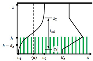
Figure 1. Schematic of time-averaged mixing layer velocity profile $\overline{u}(z)$ within a submerged canopy. The canopy height is h. The time-mean velocity at the bed and far above the canopy are denoted u₁ and u₂, respectively, with Δu = u₂−u₁. The mixing layer extends between z₁ and z₂ (_{tml = z2−z1}), with endpoints defined by $(\overline{u_{tml}}-u_1)/\text{Δ}u=0.01$ and $(u_2-\overline{u_{tml}})/\text{Δ}u=0.01,with\overline{u_{tml}}=(u_1+u_2)/2$.

Seagrass pollen has a filamentous shape, with Z. marina pollen length L_p = 3 to 5 mm and diameter B_p = 7.5e−6 m (Ackerman, 1997). The filamentous shape enhances the capture efficiency relative to spheroid pollen (de Cock, 1980; Ackerman, 2002). Z. marina is monoecious and self-compatible, producing spadices with both male and female flowers that develop acropetally along each reproductive stalk (Ackerman, 2006). Flowering shoots are slightly taller than vegetative shoots (Ackerman, 2002). Within each spathe, flower development is protogynous, which prevents self-fertilization at the scale of the inflorescence, although geitonogamy may occur across flowering shoots that are part of the same clone (e.g., Reusch, 2001; Rhode and Duffy, 2004). Successful seed production requires pollen movement among spathes and flowering shoots, and the movement of pollen is expected to be highly dependent on the location of release within the canopy, and the canopy- and landscape-scale flow structure (Kendrick et al., 2012; Follett et al., 2016).

In this paper, we numerically simulated the trajectory of individual pollen grains to examine factors that impact pollen transport and capture in a seagrass canopy, focusing on the dominant seagrass species in the northern hemisphere, Z. marina, or eelgrass. Previous work has considered the dispersal of floating seagrass seeds and propagules, including rafted seeds of Z. marina, which are spread via large-scale coastal currents (Kallstrom et al., 2008; McMahon et al., 2014; Grech et al., 2016). Here we consider transport at the meadow scale, including the vertical turbulent diffusion that carries pollen out of and into a submerged meadow. The simulation was used to explore the impact of submergence depth and pollen release height. The effect of pollen shape was also investigated, building upon previous studies of the role of filiform pollen (Ackerman, 1995, 2000). Finally, the transport trends were related to observed genetic diversity in seeds produced from paired inflorescences located at higher and lower vertical positions on the same Z. marina reproductive shoot. Recruitment from seeds is increasingly recognized as important for seagrass population dynamics as well as genetic connectivity (Kendrick et al., 2012); thus a more detailed consideration of the hydrodynamic influences on pollen transport can improve our understanding of the processes underlying successful sexual reproduction in seagrasses, and in doing so enhance future investigations of meadow genetic diversity, clonal structure and demography.

2. Methods

This study explored the dispersion of negatively buoyant particles (representing pollen) using a random displacement model (RDM) to simulate the trajectory of individual pollen grains. Within the model, the velocity profile $\overline{u}(z)$ and eddy diffusivity profile K_z(z) were predicted from canopy physical properties, including the canopy height, shoot density, blade width, and shear velocity at the top of the canopy, which is equal to the square root of the Reynolds stress at the top of the canopy, $u_{*}=\sqrt{-{\overline{u^{{}^{\prime }}{w}^{{}^{\prime }}}}_h}$ (Follett et al., 2016). Experimental observations of velocity and turbulent diffusivity in a series of rigid and flexible submerged model canopies (Ghisalberti and Nepf, 2002, 2004, 2005, 2006; Lacy and Wyllie-Echeverria, 2011) were used to validate the modeled profiles of time-mean velocity and eddy diffusivity.

2.1. Vertical Profiles of Velocity and Eddy Diffusivity Used to Parameterize RDM

The model used coordinates (x, y, z) aligned with the current, in the cross-stream direction, and normal to the bed, respectively (Figure 1). The velocity vector $\vec{u}=(u,v,w)$ corresponded to the coordinates (x, y, z), respectively. An overbar denotes a time-average. The model only considered dense canopies (ah≳0.1), representative of many Z. marina meadows (e.g., Dennison and Alberte, 1982; Chandler et al., 1996; Moore, 2004; McKone, 2009; Lacy and Wyllie-Echeverria, 2011; Infantes et al., 2012; Hansen and Reidenbach, 2013; Reidenbach and Thomas, 2018). For a dense canopy, the velocity profile within and above the canopy resembles a mixing layer, with a hyperbolic tangent profile centered slightly above the top of the canopy (Ghisalberti and Nepf, 2002):

$\begin{array}{rc}\overline{u}(z)=0.5\text{Δ}u\text{ tanh}\left(\frac{z-(h+0.5\theta )}{2\theta }\right)+0.5(u_1+u_2)& (1)\end{array}$

Here, u₁ and u₂ are the velocities at the limits of the mixing layer, z₁ and z₂, respectively, and Δu = u₂−u₁ (Figure 1). The momentum thickness of the mixing layer, θ, is related to the physical thickness of the mixing layer t_ml = z₂−z₁ = 7.1θ (Ghisalberti and Nepf, 2002). As summarized below, the empirical constants included in the mixing-layer profile (Equation 1) were estimated using measurements over nine rigid and six flexible canopies, with different frontal area density and depth-averaged velocity, the details of which are given in Ghisalberti and Nepf (2002, 2004, 2005, 2006). The height of the flexible canopies was defined as the maximum blade height as determined from video footage (Ghisalberti and Nepf, 2006). First, the velocity difference across the mixing layer (Δu = u₂−u₁) is correlated with shear velocity at the top of the canopy, u_* Specifically, $\text{Δ}u=\frac{u_{*}}{0.14}$ for rigid canopies (Ghisalberti and Nepf, 2005), and $\text{Δ}u=\frac{u_{*}}{0.11}$ for flexible canopies (based on data presented in Table 1, Ghisalberti and Nepf, 2006). Second, the lower endpoint of the mixing layer, z₁/h, increases with canopy density, with $\frac{z_1}{h}$ dependent on the canopy drag parameter, C_Dah, with C_D the canopy drag coefficient. Specifically, $\frac{z_1}{h}=0.39-\frac{0.078}{C_{D}ah}$ for rigid canopies, and $\frac{z_1}{h}=0.63-\frac{0.29}{C_{D}ah}$ for flexible canopies, based on data presented in Table 1, Ghisalberti and Nepf (2006). Third, the extent of the mixing layer region $t_{ml}=\frac{h-z_1}{0.38}$. For submergence depths less than H/h = 2, the mixing layer is restricted by the water surface, and the penetration of the mixing layer into the canopy is limited to the distance H−h from the top of the canopy (Nepf and Vivoni, 2000), so that for H/h ≤ 2, the mixing layer extends from z₁ = h−(H−h) to the water surface (z₂ = H). Fourth, the velocity in the lower canopy, u₁, is related to the velocity at the top of the meadow, u_h. Specifically, the ratio $\frac{u_1}{u_h}$ decreases with non-dimensional meadow density, ah. Specifically, $\frac{u_1}{u_h}=0.38{(C_{D}ah)}^{-0.26}$ for rigid canopies; and $\frac{u_1}{u_h}=0.21{(C_{D}ah)}^{-0.45}$ for flexible canopies (Ghisalberti and Nepf, 2006). Finally, the velocity difference across the mixing layer (Δu), normalized by the velocity at the top of the canopy u_h, is a function of the frontal area per canopy volume a and the stem diameter d ($\frac{\text{Δ}u}{u_h}=6.8{(ad)}^{0.42}$, Ghisalberti and Nepf, 2004). In order to construct velocity profiles using Equation (1), z₁ was first found using C_Dah. Next, u_* or Δu was chosen to define a specific flow condition, and u_h, u₁, and u₂ were found using the fitted relations described above.

TABLE 1

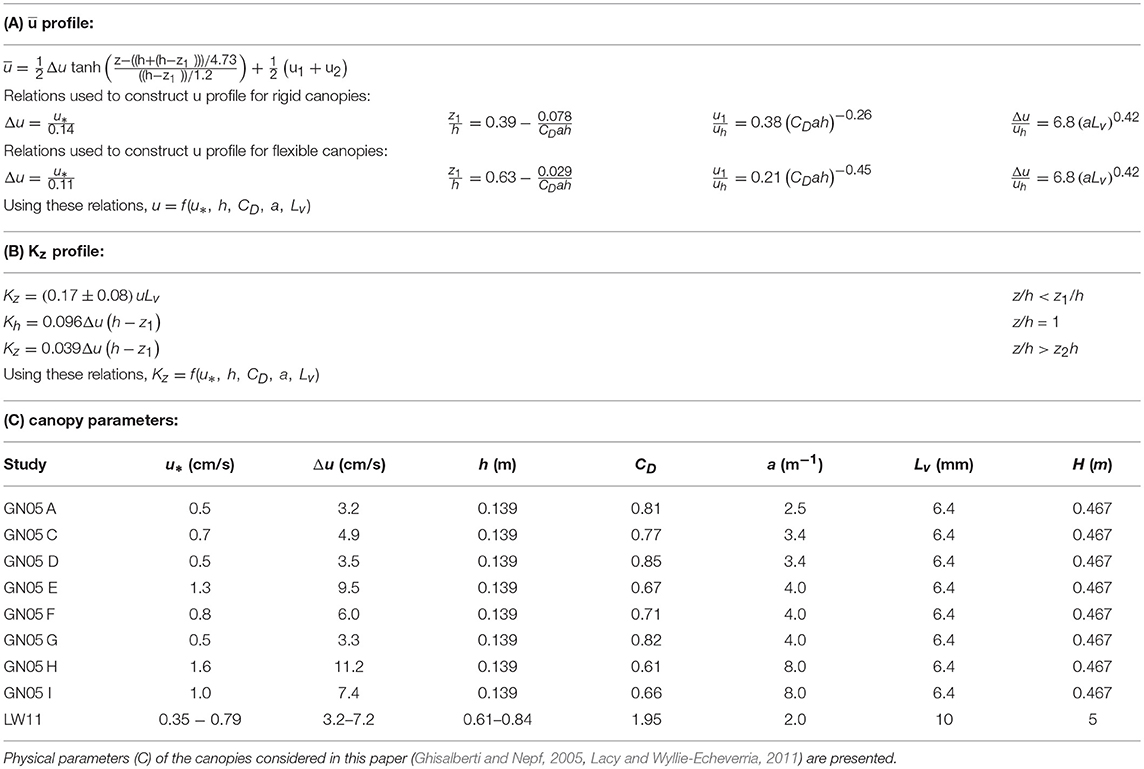
Table 1. Equations describing the curves of (A) mean longitudinal velocity and (B) eddy diffusivity, which require the canopy shear velocity, canopy height, drag coefficient, frontal area, and blade width.

The vertical profile of eddy diffusivity is divided into two regions. In the lower canopy (z < z₁), the eddy diffusivity scales with the size of the vegetation elements, L_v, which here is the seagrass blade width. For conditions that produce turbulence in the blade wakes ($\frac{u_1{L}_v}{\nu }>100$, with ν the kinematic viscosity of water), the vertical eddy diffusivity is K_z = (0.17±0.08)uL_v (Lightbody and Nepf, 2006). Within the mixing layer (h ≥ z ≥ z₁), canopy-scale vortices elevate K_z. The eddy diffusivity peaks at z = h and scales with the mixing layer thickness, t_ml, and velocity difference, Δu (K_h = 0.032Δut_ml, Ghisalberti and Nepf, 2005). When the submergence depth is low (H/h ≲ 5), the eddy diffusivity has a constant value (K_z = 0.013Δut_ml) above the mixing layer (z > z₂) (Ghisalberti and Nepf, 2005). The eddy diffusivity was assumed to follow a linear function between the regions of constant diffusivity (z₁ > z > z₂) and z = h. An example of a K_z profile is included in Figure 1. Lateral transport was assumed to be dominated by blade-scale turbulence, so that the lateral diffusivity was assumed to be equal to K_y = (0.17±0.08)uL_v. For validation of the method, the vertical profiles of velocity and diffusivity predicted from the above relationships across a range of canopy densities are compared to measured velocity and eddy diffusivity from experiments reported in Ghisalberti and Nepf (2005, Figure 2). On average, the predicted profiles agreed with the measurements to within 10%.

FIGURE 2

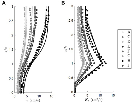
Figure 2. Family of vertical profiles for the (A) time mean longitudinal velocity and (B) eddy diffusivity over a submerged rigid canopy of increasing shoot density. The circles represent the measured values from Ghisalberti and Nepf (2005), and the predicted profiles are shown with solid lines. The colors denote different experimental case. In alphabetical order of experimental run, u_* = 0.45, 0.74, 0.53, 1.33, 0.84, 0.50, 1.57, 0.86, 0.55 cm/s, C_D = 0.81, 0.77, 0.85, 0.67, 0.71, 0.82, 0.61, 0.66, 0.79, and a = 0.025, 0.034, 0.034, 0.040, 0.040, 0.040, 0.080, 0.080, 0.080 cm⁻¹. For all cases the canopy height was h = 13.9 cm and the plant width was L_v = 0.64 cm.

2.2. Random Displacement Model (RDM) for Particle Transport

Within the random displacement model (RDM), individual particles originated at a specific source height within the meadow (0 < z<h) and were tracked until they deposited on the canopy, settled to the bed, or left the model domain. The size of the model domain in the directions (x, y, z) was (200h, 20h, H). In each time-step (Δt) the position of the particle (x_p, y_p, z_p) advanced longitudinally with the mean velocity $\overline{u}(z)$ and vertically due to both settling (w_s) and turbulent eddy velocity (w′). The equations used to model the particle position were (Wilson and Sawford, 1996):

$\begin{array}{rcll}{x}_{p,i+1}& =& x_{p,i}+\overline{u}(z_{p,i})\text{Δ}t& (2)\end{array}$

$\begin{array}{rcll}{y}_{p,i+1}& =& y_{p,i}+R_y\sqrt{2K_y(z_{p,i})\text{Δ}t}& (3)\end{array}$

$\begin{array}{rcll}{z}_{p,i+1}& =& z_{p,i}+\left(\frac{d{K}_z\left(z_{p,i}\right)}{dz}-w_s\right)\text{Δ}t+R_z\sqrt{2K_z\left(z_{p,i}\right)\text{Δ}t}& (4)\end{array}$

The last term in (3) and (4) represents transport by turbulent velocity $v^{\prime }=R_y\sqrt{2K_y}/\sqrt{t}$ and $w^{\prime }=R_z\sqrt{2K_z}/\sqrt{t}$, respectively, with R_y, R_z random numbers drawn from a normal distribution with mean 0 and standard deviation 1. The vertical transport (Equation 4) also included a drift correction, or pseudo-velocity, associated with the vertical variation in diffusivity (dK_z/dz). The pseudo-velocity term prevented the artificial accumulation of particles in regions of low diffusivity (Durbin, 1983; Wilson and Yee, 2007). The formulations for $\overline{u}(z)$, K_y(z) and K_z(z) were described in the section Vertical Profiles of Velocity and Eddy Diffusivity used to Parameterize RDM. The particle position was saved at every time-step. The constant model time-step, Δt, was constrained so that the vertical particle excursion within each time-step was much smaller than the scale of vertical gradients in the diffusivity and velocity (Israelsson et al., (2006). Within the canopy, both the velocity and diffusivity varied over length scales of approximately 0.1h. Within each time-step, after a particle was moved, the position was assessed to determine if the particle had settled to the bed (z_{p, i} = 0), reached the water surface (z_{p, i} = H), traveled beyond the model domain (x_{p, i} > 200h, |y_{p, i}| > 20h), or deposited to the canopy.

Z. marina pollen contains a sticky coating, increasing adherence to surfaces contacted by the pollen grains (de Cock, 1980). Based on this, the canopy capture model used for this study assumed that all pollen particles contacting vegetation surfaces were captured and ceased further transport. Canopy deposition was described as the probability of capture of one particle in one time-step, found from the probability that the particle was located upstream of the projected area of a blade, multiplied by the capture efficiency, or the fraction of particles removed from the volume of water passing the projected area of the blade (Palmer et al., 2004). The probability that the particle was upstream of the projected area of a blade was equal to the blade width L_v = 0.0055 m (McKone, 2009) divided by the average center-to-center spacing between blades (ΔS) (Figure 3A). In addition, successful canopy capture required that the particle be located close enough to the blade so that it could impact the blade within one time-step, which was equal to the longitudinal particle excursion in one time-step $(\text{Δ}{x}_{p,i}=\overline{u}(z_{p,i})t)$ divided by the average longitudinal spacing between blades (ΔS). The capture efficiency (η) was based on the measured efficiency for particle impaction on rigid cylinders coated with Vaseline (Palmer et al., 2004), assuming that the blade width could be substituted for the cylinder diameter:

$\begin{array}{rc}\eta =0.224{R{e}_c}^{0.718}{R_p}^{2.08}& (5)\end{array}$

with the collector Reynolds number $R{e}_c=\frac{\overline{u}{L}_v}{\nu }$. The particle ratio $R_p=\frac{d_p}{L_v}$ is the ratio of the particle diameter (d_p) to the blade width, so that Equation (5) indicates that the capture efficiency increases with increasing particle diameter. The impact of pollen grain shape was explored by simulating both filamentous and spherical pollen grains with the same settling velocity and volume. The filamentous pollen grains were given the following attributes based on Ackerman (2002): w_s = 3.5e−6 m/s, L_p = 4e−3 m, B_p = 7.5e−6 m. The spherical pollen grains were given the same settling velocity as the filamentous grains and diameter d_p = 3.5e−5 m. To adapt Equation (5) for the filamentous pollen, an effective pollen diameter was determined in the following way. The pollen filaments rotate continuously (Ackerman, 1997), with the pollen having equal probability of assuming any rotation angle (γ, ϕ) from the (x, y, z) axes, such that all possible pollen endpoints were evenly distributed over the surface of a sphere. Within each time-step, the effective pollen diameter was assumed to be the projected length of the pollen on the y-axis, so that a pollen grain with its long axis aligned with the y-axis would have an effective diameter equal to L_p and a pollen grain with its long axis aligned with the x-axis would have an effective diameter equal to the diameter of the pollen, B_p. At each time step, a new particle rotation angle was chosen for each particle from a uniform distribution of all possible pollen positions. Specifically, j and k were chosen from a uniform distribution on (0, 1). Then

$\begin{array}{rc}\gamma =2\pi j& (6)\end{array}$

$\begin{array}{r}\varphi ={\mathit{\text{cos}}}^{-1}(2k-1) (7)\end{array}$

The effective pollen diameter was equal to the Cartesian transformation of the pollen position from spherical coordinates, d_p = L_p sin γsinϕ (Edwards and Penney, 2002). Using this model, a pollen grain perpendicular to the y-axis would have diameter 0. In order to accommodate the finite width of real pollen grains, the minimum effective diameter was set equal to B_p.

FIGURE 3

Figure 3. (A) Diagram of pollen grain approaching three blades shown in cross-section. The blade width is L_v and the center-to-center spacing between blades is ΔS. (B) Diagram of blade posture and determination of projected area in the x direction. The curved blade posture was broken into a series of linear segments, such that the blade position was converted to a series of vectors. The cosine of the angle between the blade orientation g(z) and the vertical vector f was found by dividing the dot product of f and g(z) by the magnitudes of both vectors.

Multiplying the capture efficiency by the probability that the particle is in the plane of the blade and close enough to contact the blade in one time-step, the probability of particle impaction on a blade surface in one time-step is:

$\begin{array}{rc}d{p}_x=\eta \frac{L_v}{{\text{Δ}S}^2}\text{Δ}{x}_{p,i}=\eta a_x\text{Δ}{x}_{p,i}& (8)\end{array}$

with (a_x) the component of the one-sided blade area projected in the x direction. Similarly, the probability of particle impaction on horizontal surfaces is dp_z = min(0, ηa_zΔz_{p, i}), with the impact of gravitational settling and turbulent transport included in the vertical particle excursion Δz_{p, i} (Equation 2). Particle impaction on lateral surfaces was neglected due to the relatively smaller blade thickness (1 mm).

We used equation 4 in Luhar and Nepf (2011) to describe the current-induced changes in seagrass blade position. To find the component of the blade area projected in the x and z directions at each vertical position, the curved blade posture was broken into linear segments, such that the blade surface was converted to a series of vectors (Figure 3B). The projected area in the x direction, P_x(z), was found by multiplying the magnitude of the vector segment by the cosine of the angle (cosθ) between the vertical vector (f) and the blade position (g(z)) found by dividing the dot product of f and g(z) by the magnitudes of both vectors ($cos\theta (z)=\frac{f·g(z)}{\left|f\right|\left|g(z)\right|}$, Figure 3B). Similarly, the projected area in the z direction, P_z(z), was found by multiplying the magnitude of the vector segment by the sine of the angle (sin(θ)) between the blade position and the vertical vector. The component of the blade area projected in the x and z directions was found by multiplying the one-sided blade area (a) by P_x(z) and P_z(z), respectively. The probability of particle deposition was the sum of the probability of particle impaction on both the vertical and horizontal surfaces (dp = dp_x+dp_z). To determine if the particle deposited to the canopy during the time-step, a random number, R_c, was chosen from a uniform distribution between 0 and 1. If R_c was less than or equal to the probability of deposition, the particle deposited to the canopy.

The RDM model was validated using measured profiles of dye concentration along a rigid model canopy (case I in Ghisalberti and Nepf, 2004). The dye was released at x/h = 0 and z/h = 1 and measured at six downstream longitudinal locations (x/h = 1.4, 3.9, 6.6, 10.8, 18.0, 27.3). To represent the neutrally buoyant tracer, the RDM particles were given neutral buoyancy (w_s = 0), retention on canopy elements was omitted, and the bed and water surface (z = 0, H) were treated as no-flux boundaries. In order to calculate simulated concentration and mass flux, a vertical column of interrogation boxes (0.02 m long × 0.01 m high) was defined, centered at the longitudinal measurement points. Particles were continuously released until a steady-state particle concentration was established in each box. The concentration, C(z), was found by dividing the steady-state number of particles in each box by the box volume. The mass flux was found by integrating the flux at each box over the water depth, $Q_x=\int \overline{u}(z)C(z)dz$.

The validated transport model was used to explore the influence of several factors on pollen transport, including pollen release height within the canopy, pollen shape, interaction with the water surface, submergence depth ratio (H/h), and depth-average velocity. The flexible meadow parameterizations were used in order to represent the reconfiguration of real seagrass. The selected range of submergence, H/h = 5, 4, 3, 2, 1.5, represented the range observed for Z. marina canopies at our field sites near Nahant and Gloucester, MA, where H/h = 1.5 to 6.25 at the shallow and deep canopy edges. In the field, pollen grains have sometimes been observed to collect at the water surface, forming a connected floating layer that restricts future transport (de Cock, 1980), while in other instances pollen collected at the surface returned to the water column due to wave and wind action (Ducker et al., 1978; Ruckelshaus, 1996; Ackerman, 1997). These two conditions were represented in the simulation by different surface boundary conditions. On the one hand, the return of pollen from the water surface into the water column was represented as a no-flux, or reflecting, boundary. On the other hand, the collection of pollen on the water surface was represented as an absorbing (perfect sink) boundary condition. For all cases, the pollen was released at the top of the canopy (z/h = 1).

2.3. Genetic Diversity of Seeds Produced on Paired Upper and Lower Inflorescences

Flowering shoots were selected haphazardly, at least 5 meters apart at a depth of approximately 3 m MLLW, from the interior of two Z. marina meadows in northern Massachusetts (Dorothy Cove, Nahant, and Niles Beach, Gloucester). Canopy height (h) ranged from 85 to 135 cm, so that H/h > 2 for all samples. From each flowering shoot (n = 7; 3 from Nahant and 4 from Gloucester), we collected a leaf sample and 6–10 developing seeds from each of two spathes, one from the highest rhipidia and one from the lowest, and the location of those spathes were recorded as the distance above the substrate of the midpoint of the inflorescence. Maternal leaf tissue was frozen at −20°C until DNA extraction; seeds were frozen at −80°C. DNA was extracted from leaves by grinding each sample with a Retsch mixer mill MM400 and using the Omega Bio-Tek E.N.Z.A.^® Plant DNA Kit. Individual seeds were ground by hand in microfuge tubes with micro-pestles and DNA was extracted with Chelex 100 (Bio-Rad); samples were incubated at 55°C for 8–24 h, gently mixed, heated to 98°C for 10 min, vortexed, centrifuged at 14,000 rpm for 5 min, and the supernatant stored at −20°C until PCR.

Each seed and maternal shoot was genotyped using 8 microsatellite loci developed for Z. marina and known to be polymorphic for these populations, multiplexed in 3 11 μl PCR reactions (Table 1). Each reaction consisted of 1 μl DNA template, 5 μl 2X Type-It multiplex master mix (Qiagen), and 0.25 μl of each 10 μM primer. PCR cycling conditions included initial activation/denaturation at 95°C for 5 min, followed by 28 cycles of 95°C for 30 s, 60°C for 90 s, and 72°C for 30 s, and final extension at 60°C for 30 min. PCR products were separated on a 3730xl Genetic Analyzer (Applied Biosystems) and fragment analysis was performed using GeneMarker version 2.6 (SoftGenetics).

To compare seed diversity across samples that differed in size (n = 6 to 10 seeds per spathe), we calculated allelic richness (A_E) rarified to the smallest sample size (i.e., 12 alleles) using the program HP-RARE (Kalinowski, 2005). The program GERUD 2.0 (Jones, 2005) was used to determine the number of unique fathers contributing to each seed set. GERUD uses an exclusion approach to determine the minimum number of sires necessary to produce a given progeny array when the mother's genotype is known, as in our data set. If a progeny array was too complex to solve using all 8 loci, we removed the least informative locus until a solution could be found (Jones, 2005); pairs of inflorescences from the same maternal shoot were always analyzed with the same set of loci. We divided the minimum number of unique fathers by the number of seeds genotyped to standardize comparisons across inflorescences with different numbers of seeds and used paired t-tests to compare the diversity of seeds produced on high vs. low inflorescences on each flowering shoot.

3. Results

3.1. Validation of RDM Model

The simulation was validated against vertical profiles of dye concentration measured along a rigid model canopy (case I in Ghisalberti and Nepf, 2004). To mimic the real tracer, the model particles were assumed to be neutrally buoyant (w_s = 0). The measured and modeled concentration fields displayed similar vertical dispersion for x/h ≥ 3.9, where the measured and modeled observations agreed to within 7% (Figure 4). However, closer to the source, x/H = 1.4, the modeled concentration (Figure 4, open squares) exhibited greater vertical dispersion than the measured concentration (Figure 4, solid circles), as the modeled concentration spread over a larger vertical distance with a reduced peak magnitude relative to the measured concentration. The initially smaller rate of dispersion for the real tracer can be explained by the presence of multiple eddy scales within the real system. The vertical distribution of real tracer was initially influenced by turbulence scales smaller than the canopy-scale vortices, and thus experienced slower diffusion. The canopy-scale vortices did not contribute to the diffusion of the real tracer until the real tracer cloud grew to a size comparable to the canopy-scale vortices. In contrast, the simulation applied a constant diffusivity based on the canopy-scale vortices, so that the tracer was effectively influenced by the largest scale of turbulence from the point of release, and thus initially dispersed more rapidly than the real tracer.

FIGURE 4

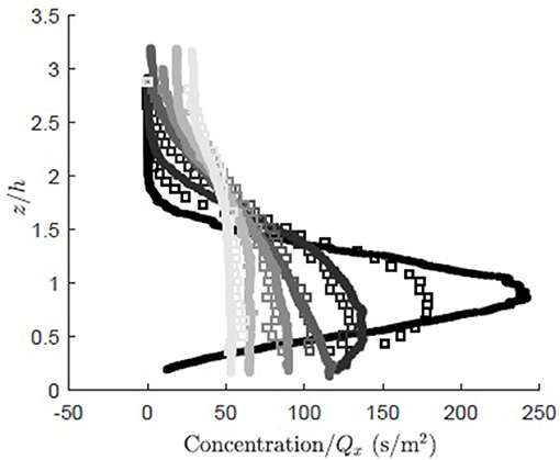
Figure 4. Comparison of concentration normalized by total mass flux for RDM particles (open squares) and measured dye concentration (solid dots, case I, Ghisalberti and Nepf, 2005) at six longitudinal locations (x/h = 1.4, 3.9, 6.6, 10.8, 18.0, 27.3, dark to light gray). The concentration (g/m²) was normalized by the longitudinal flux, $Q_x=\int \overline{u}(z)C(z)dz$ (g/s).

3.2. Validation of Velocity Model

The velocity model was also validated with field measurements in a Z. marina meadow, as reported in Lacy and Wyllie-Echeverria (2011, site ED3). The velocity profile was measured at 3 time points over a tidal cycle, resulting in different depth-average velocity and canopy height h = 0.84, 0.78, 0.61 m and ΔU = 0.032, 0.050, 0.072 m/s (Figure 5, open circles, triangles, and squares). The frontal area per canopy volume a = 2 m⁻¹ was computed for vertical blades from measurements of blade dimensions and shoot density, with blade width L_v = 1 cm. The frontal area per canopy volume was assumed to be constant over the reconfigured canopy height h. As a canopy composed of flexible blades reconfigures, there is decrease in drag predominantly because the pronated component of the blades contribute little to drag. Luhar and Nepf (2011) demonstrated that the drag imparted by a flexible blade can be represented as an equivalent rigid blade of shorter length, called the effective blade length, l_e. Since the effective blade is rigid, its imparted drag is described by the drag coefficient for a rigid blade, C_D = 1.95 (Luhar and Nepf, 2011). We assumed that the deflected meadow height (h) was a reasonable approximation for the effective blade length, but acknowledge that this may produce a slight over prediction, based on the comparison shown in Figure 2 in Luhar and Nepf (2013). The canopy was assumed to be deeply submerged (H/h>2) based on the reported site elevation of −2 m MLLW. The modeled velocity profile (Figure 5, solid, dashed, and dash-dot lines) agreed with the measurements to within a maximum difference of 3.8%.

FIGURE 5

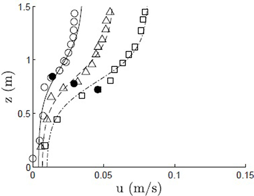
Figure 5. Modeled (solid, dashed, and dash-dot lines) and measured (open circles, triangles, and squares) velocity profiles within a Z. marina canopy (Shaw Island, WA; Lacy and Wyllie-Echeverria, 2011) at three points during a tidal cycle, with canopy height h = 0.84, 0.78, 0.61 m, denoted by solid black dot, and ΔU = 0.032, 0.050, 0.072 m/s, L_v = 1 cm, C_D = 1.95, and a = 2 m⁻¹.

The likelihood of outcrossing vs. selfing will depend on the relationship between mean clone size (i.e., the area covered by a given genotype) and the pollen dispersal kernel, both of which will vary among seagrass meadows. However, all else being equal, increased within-meadow pollen dispersal will increase opportunity for pollen to encounter non-self-flowers. Therefore, we are interested in what attributes of the meadow impact the maximum distance traveled before canopy capture. The validated model was used to explore the impact of different flow and morphology parameters on pollen transport. The effect of submergence depth, depth-average velocity, pollen shape, and pollen release height were explored, with canopy parameters a = 2 m⁻¹, h = 1 m, L_v = 1 cm, C_D = 1.95 remaining constant for all simulations.

3.3. Influence of Submergence Depth H/h on Pollen Transport

The simulation was used to understand the impact of submergence depth on long-distance pollen transport. Filamentous particles were released at z_rel/h = 1 for submergence depths H/h = 1.5, 2, 3, 4, 5 in a canopy with u_* = 0.01 m/s. As discussed in the methods, two surface boundary conditions were considered, particles rebounding off the water surface (Figure 6) and particles captured by the water surface (Figure 7). For all submergence depths and for both surface boundary conditions, the number of particles in the water column, N, most of which were above the canopy, decreased with the same dependence on distance, N ~ x^−1/2 (Figures 6, 7). This dependence arose because the canopy was a strong sink for pollen, so that the in-water concentration of particles was close to zero within the canopy. Then, the loss of particles to the canopy, ∂N/∂x, depends on the vertical turbulent flux of particles toward the canopy, which in turn depends on the vertical gradient of particle concentration, ∂C/∂z, above the canopy, i.e., ∂N/∂x ~∂C/∂z. The remaining particles, N, are distributed above the canopy over the vertical length-scale for diffusion, ${\delta }_z~x^{-1/2}$, such that the mean concentration above the canopy is C_mean~N/δ_z. Since the concentration is close to zero in the canopy, $\partial C/\partial z~C_{mean}/{\delta }_z~N/{\delta }_z^2~N{x}^{-1}$. Since ∂N/∂x~∂C/∂z, we can also write ∂N/∂x~Nx⁻¹, which has the solution N~x^−1/2.

FIGURE 6

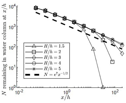
Figure 6. Number of particles remaining in the water column with distance from the release point x_rel/h = 0 for 10,000 filamentous particles released at z_rel/h = 1 in a canopy (u_* = 0.01 m/s, L_v = 1 cm, a = 2 m⁻¹, C_D = 1.95, h = 1 m) with varied submergence depth, H/h = 1.5, 2, 3, 4, 5, respectively, represented by open triangles, squares, diamonds, circles, and asterisks. Particles were evaluated at 10 points spaced equally in log space, (x/h = 0.05, 0.13, 0.32, 0.80, 2.0, 5.0, 13, 32, 80, 200). Particles reaching the water surface (z/h = H/h) were reflected off of the surface boundary, remaining available for transport within the water column and the possibility of capture on canopy elements. A line illustrating a power law with decay constant −1/2 is plotted for reference (black dashed line).

FIGURE 7

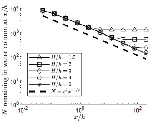
Figure 7. Number of particles remaining in the water column with distance from the release point x_rel/h = 0 for 10,000 filamentous particles released at z_rel/h = 1 over a canopy (u_* = 0.01 m/s, L_v = 1 cm, a = 2 m⁻¹, C_D = 1.95, h = 1 m) with varied submergence depth, H/h = 1.5, 2, 3, 4, 5, respectively, represented by open triangles, squares, diamonds, circles, and asterisks. Particles were evaluated at 10 points spaced equally in log space, (x/h = 0.05, 0.13, 0.32, 0.80, 2.0, 5.0, 13, 32, 80, 200). Particles reaching the water surface (z/h = H/h) were considered to be adhered to that boundary, but remaining within the water column. A line illustrating a power law with decay constant −1/2 is plotted for reference (black dashed line).

The particle number (N) deviated from the x^−1/2 dependence when the particles began to interact with the water surface. For the reflecting boundary condition (Figure 6), the loss of particles to the canopy was accelerated, because the reflected particles were forced back toward the canopy. For example, for the smallest submergence depth, H/h = 1.5 (triangles in Figure 6), this transition occurred at x/h = 5, at which point a significant fraction of the particles (26%) had interacted with the surface. For the absorbing boundary condition (Figure 7), the transition in particle loss occurred at the same x-positions (i.e., x/h = 5 for H/h = 1.5), but once the particles were captured by the water surface, capture by the canopy ceased, so that the number of particles in the water column stopped decreasing. Particles trapped at the surface could remain in the water column until wave breaking or wind-generated turbulence knocked them free of the surface layer, making them available again for canopy capture. Although wavebreaking is not included in the model, this implied that capture at the water surface is a mechanism that enhanced long-distance dispersal.

Note that the comparisons made in Figures 6, 7 assume the same depth-average velocity for all submergence ratios, whereas in the field, water depth and current speed are typically correlated through the tidal cycle. Therefore, the maximum transport of pollen in the field may not occur at high tide (maximum submergence ratio), but at some intermediate point in the tide with higher velocity. Nevertheless, the general trend of greater pollen transport at greater water depths (greater H/h) would be valid when comparing a meadow across a depth gradient.

3.4. Influence of Velocity Variation

The impact of variation in the depth-average velocity was considered by varying the canopy shear velocity between u_* = 0.001 and 0.02 m/s, based on the range of u_* found in four Z. marina meadows (Grizzle et al., 1996; Lacy and Wyllie-Echeverria, 2011). Filamentous particles were released in a canopy with H/h = 5, z_rel/h = 1, and a reflecting surface boundary condition. Increasing u_* was associated with an increase in depth-averaged velocity, U, which spanned 0.8 to 17 cm/s, respectively, for the u_* values given above. The vertical diffusivity within the mixing layer was linearly proportional to Δu and thus u_*, and for the range of u_* values spanned K_{z, h} = 4 to 80 cm²/s², respectively. Because the velocity has higher values above the canopy and lower values within the canopy (Figure 5), particles that initially escaped the meadow and traveled for some distance above the meadow, where capture could not occur, had the greatest travel distances. The average distance traveled divided by the time spent above the canopy (z/h ≥1) was 0.97, 4.8, 19 cm/s, which was close to the average longitudinal velocity above the canopy for each u_* condition ($\overline{u}{|}_{H-h}=0.99,4.9,20$ cm/s), indicating that longitudinal transport predominantly occurred when particles were located above the canopy.

Particles released in canopies with higher depth-averaged velocity had only slightly greater travel distances. This is shown by a slightly higher number of particles remaining in the water column for larger values of u_* at each distance from the release (Figure 8). Similarly, increasing the depth-average velocity from 0.8 to 17 cm/s increased the number of particles reaching the end of the domain only slightly, from 86 to 146 (Figure 8). That is, increasing U by a factor of about 20 only increased the number of particles leaving the domain by a factor of about 2. The weak dependence of travel distance on depth-average velocity can be explained by the linear dependence of K_z on the velocity shear (Δu) and thus on the depth-average velocity (U). Specifically, the ratio K_z/U was roughly a constant. Therefore, although increasing U allowed particles above the meadow to advect more quickly away from the source, a comparable increase in K_z enhanced particle flux into the meadow, so that the spatial rate of particle capture by the meadow had little dependence on depth-average velocity.

FIGURE 8

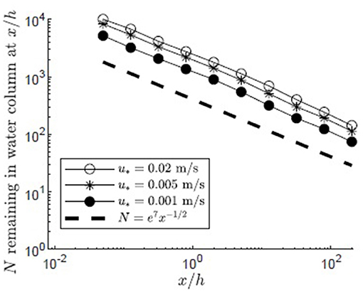
Figure 8. Number of particles remaining in the water column with distance from the release point x_rel/h = 0 for 10,000 filamentous particles released at z_rel/h = 1 over a canopy (H/h = 5, L_v = 1 cm, a = 2 m⁻¹, C_D = 1.95, h = 1 m) with varied canopy shear velocity, u_* = 0.001, 0.005, 0.02 m/s, respectively, represented by black circles, asterisks, and open circles. Particles were evaluated at 10 points spaced equally in log space, (x/h = 0.05, 0.13, 0.32, 0.80, 2.0, 5.0, 13, 32, 80, 200). A line illustrating a power law with decay constant −1/2 is plotted for reference (black dashed line).

3.5. Influence of Pollen Shape

Pollen shape significantly influenced the maximum distances traveled by pollen. Using the same meadow and release conditions (H/h = 5, z_rel/h = 1, reflecting surface boundary, u_* = 0.01 m/s), the transport of filamentous pollen (L_p = 4e−3 m, B_p = 7.5e−6 m) was compared to that of spherical pollen grains of the same volume and settling velocity, but diameter d_p = 3.5e−5 m (Figure 9). The filamentous pollen had significantly higher canopy capture rates, resulting in more of the filamentous pollen remaining closer to its release point. Specifically, for the filamentous pollen over 98% of the pollen was captured by the canopy before the end of the modeled domain, and no particles reached the bed (z = 0). In addition, the filamentous pollen remaining in the water column decays following the x^−1/2 dependence, which is consistent with the canopy behaving as a nearly perfect sink (see discussion in section Influence of Submergence Depth H/h on Pollen Transport). In contrast, the spherical pollen was not as efficiently captured by the canopy, and as a result the spatial decline in water column pollen was much slower and specifically did not follow the x^−1/2 dependence. Further, only 54% of the spherical pollen grains were captured by the canopy within the modeling domain, and 46% of particles traveled beyond the end of the modeling domain.

FIGURE 9

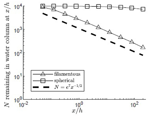
Figure 9. Number of filamentous (open triangles) and spherical (open squares) particles remaining in the water column with distance from the release point x_rel/h = 0 for 10,000 particles released at z_rel/h = 1 over a canopy (H/h = 5, u_* = 0.01 m/s, L_v = 1 cm, a = 2 m⁻¹, C_D = 1.95, h = 1 m) with a reflecting water surface boundary. Particles were evaluated at 10 points spaced equally in log space, (x/h = 0.05, 0.13, 0.32, 0.80, 2.0, 5.0, 13, 32, 80, 200). A line illustrating a power law with decay constant −1/2 is plotted for reference (black dashed line).

3.6. Influence of Pollen Release Height, z_rel/h

Vertical diffusivity was elevated by canopy-scale vortices within the canopy mixing layer, z₁ ≤ z ≤ z₂. The importance of this region of elevated diffusivity to pollen transport was explored by varying the pollen release height. The lowest release point (z_rel/h = 0.25, Figure 10) was below the mixing layer (z_rel/h<z₁/h = 0.49) in a region of reduced diffusivity dominated by blade-scale turbulence. The middle release point (z_rel/h = 0.75, Figure 10) was within the region affected by both blade-scale and canopy-scale turbulence, which significantly elevated the vertical diffusivity relative to the lower canopy region (Figure 3). The highest release point was z_rel/h = 1, reflecting the location of the highest inflorescences observed within coastal Massachusetts Z. marina canopies [Dorothy Cove, Nahant, MA; Niles Beach, Gloucester, MA; Woods Hole, MA (Ackerman, 1986)]. For the lowest release point (z_rel/h = 0.25), significant canopy capture (63%) occurred close to the release point (x/h < 0.05). Because the vertical diffusivity was low in this region and the release point was far from the top of the canopy, no pollen escaped the canopy from this release point. Specifically, none of the particles traveled more than x/h = 0.43, or roughly 0.43 m. Further, the maximum vertical position achieved by pollen released near the bed was only z/h = 0.29, indicating that pollen released below the mixing layer remained below the mixing layer. The fraction of particles remaining in the water column followed an exponential decay curve, reflecting first-order decay due to the distributed sink formed by the canopy elements. The capture of pollen over such small length-scales makes self-pollination likely. In contrast, at the highest release point (z_rel/h = 1), the pollen experienced both higher vertical diffusivity and proximity to the canopy top, both of which facilitated the particles being quickly carried above the canopy, allowing them to avoid canopy capture and experience higher current speeds. Together, this produced much greater travel distances. Specifically, 9% of the pollen released at $\frac{z_{rel}}{h}=1$traveled beyond x/h = 5 before canopy capture occurred, with 1.2% (120 particles) reaching the longitudinal extent of the model domain (L = 200h). The tendency to travel greater distances before capture reduces the probability of self-pollination and enhances the probability of genetically diverse, outcrossed seeds. The particles released within the upper canopy region initially followed an exponential decay curve due to the distributed canopy deposition sink, similar to the decay of the particles released at z_rel/h = 0.25 (Figure 10, open squares and diamonds). However, some particles were able to travel above z = h, after which particle deposition followed the pattern of diffusion to a boundary sink, similar to the release at z_rel/h = 1, with the number of particles decreasing with x^−1/2.

FIGURE 10

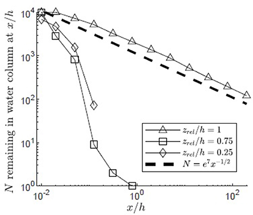
Figure 10. Number of particles remaining in the water column with distance from the release point x_rel/h = 0 for 10,000 filamentous particles released in a canopy (H/h = 5, u_* = 0.01 m/s, L_v = 1 cm, a = 2 m⁻¹, C_D = 1.95, h = 1 m) with varied release heights (z_rel/h = 1, 0.75, 0.25) and a reflecting surface boundary. Particles were evaluated at two locations (x/h = 0.01, 0.02) chosen to occur before the location of first deposition of particles from the lower release points and 10 points spaced equally in log space, (x/h = 0.05, 0.13, 0.32, 0.80, 2.0, 5.0, 13, 32, 80, 200). A line illustrating a power law with decay constant −1/2 is plotted for reference (black dashed line).

3.7. Genetic Diversity of Seeds Produced on Paired Upper and Lower Inflorescences

All eight loci used were polymorphic, displaying 3-7 alleles with a mean of 5.75 alleles locus⁻¹. We obtained complete multi-locus genotypes for 125 seeds from seven maternal half-sibling families. The majority of seeds showed Mendelian evidence of outcrossing (i.e., non-maternal alleles at one or more loci), with only 15 of 125 seeds (12%) possessing genotypes consistent with geitonogamous selfing; twice as many of these were found on lower inflorescences than on upper ones (10 vs. 5). Pooling data from both field sites and using a paired approach, we found that both measures of seed diversity tested were greater for inflorescences closer to the top of the canopy. Allelic richness (mean number of alleles per loci) was significantly greater for seeds produced in spadices close to the top of the canopy than those produced lower on the shoot (mean and standard deviation 2.87 ± 0.24 vs. 2.60 ± 0.41; one-tailed paired t-test, p = 0.013), and the difference in allelic richness between sibling seed cohorts tended to increase with increasing linear distance between spadices (Figure 11). Likewise, the minimum number of unique fathers was greater for seed families collected from upper spadices than from lower ones (3.52 vs. 2.93 fathers/10 seeds; one-tailed paired t-test, p = 0.052).

FIGURE 11

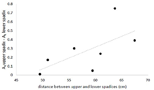
Figure 11. Difference in allelic richness between seeds collected from upper- and lower-most spadices (rarified to the smallest sample size) increased with increasing distance between inflorescences. n_seed = (6 to 10 seeds/spadix) x (2 spadices/maternal shoot) x (7 maternal shoots). Data is available from the authors upon request.

4. Discussion

Although vegetative growth historically has been assumed to be the primary mode of reproduction in seagrasses, multiple lines of evidence suggest that recruitment from seed is both more common and more important than previously believed (Kendrick et al., 2012). For example, significant variation in genetic and genotypic diversity has been documented within and among natural seagrass beds (Williams and Orth, 1998; Olsen et al., 2004; Hughes and Stachowicz, 2009), and disturbed seagrass meadows often recover at a rate faster than could occur with vegetative propagation alone (Orth et al., 2006). Further, there is increasing evidence that the genetic diversity and relatedness of seeds influences resulting seedling performance, which highlights the importance of a diverse pollen supply. The fitness costs of self-pollination in Z. marina vary among populations, but experimentally selfed inflorescences often show significantly lower seed set (Ruckelshaus, 1995; Reusch, 2001; Rhode and Duffy, 2004) and reduced seed germination compared to outcrossed inflorescences (Ruckelshaus, 1995; Billingham et al., 2007). The positive effect of seed diversity can be seen beyond the dichotomy of selfed vs. outcrossed: increased allelic richness in seeds has been shown to increase both primary and secondary production in the field (Reynolds et al., 2012), and genetically diverse, non-sibling seeds outperformed sibling seeds in a greenhouse mesocosm experiment (Randall Hughes et al., 2016). Thus, the physical processes that affect pollen delivery in the nearshore environment impact both seed quantity and quality, and this can have important ramifications for population dynamics and genetic structure in eelgrass meadows.

The transport distances achieved by the simulated pollen in our model reflected the vertical structure of turbulence within the canopy. Specifically, longitudinal transport over distances greater than x/h = 2 was only possible for pollen released within the region of the upper canopy influenced by canopy-scale vortices (z>z₁). The elevated vertical diffusivity within this region carried pollen above the canopy where it experienced higher current speeds and avoided canopy capture until additional longitudinal transport had occurred (Figure 10). Observations in real eelgrass canopies suggest that Z. marina inflorescences are located in the vertical zone influenced by canopy scale vortices, suggesting that reproductive stalk resources were directed toward release points that can benefit from higher vertical diffusivity. For example, at our field site, the lowest spadices ranged from z/h = 0.36 to 0.64 in meadows for which the corresponding z₁/h = 0.31 to 0.53 was estimated based on the non-dimensional meadow density, $\frac{z_1}{h}=0.63-\frac{0.29}{C_{D}ah}$. That is, the spadices were all located within the zone influenced by canopy-scale vortices, z > z₁. Similarly, the vertical extent of inflorescences in a Z. marina canopy reported by Ackerman (1986) extended from $\frac{z}{h}=0.3$ to 1, which corresponds with z/h > z₁/h = 0.31, estimated from the non-dimensional meadow density (ah). Over the range of reported dimensionless Z. marina meadow densities (ah = 0.1–3, based on data provided in Dennison and Alberte, 1982; Chandler et al., 1996; Moore, 2004; McKone, 2009; Lacy and Wyllie-Echeverria, 2011; Infantes et al., 2012; Hansen and Reidenbach, 2013; Reidenbach and Thomas, 2018), z₁/h = 0 to 0.6. This suggests that in some sparse canopies (ah ≾ 0.5), the canopy-scale vortices penetrate to the bed (z₁ = 0) and spadices over the entire meadow would experience elevated diffusivity. However, for dense canopies, inflorescences located below z₁would experience reduced diffusivity, resulting in much shorter distances for pollen transport.

The effect of vertical flow structure observed in the model can also be seen in our empirical data on seed diversity. Seeds collected from lower inflorescences had reduced allelic richness relative to seeds produced from higher inflorescences on the same flowering shoot (Figure 11), consistent with the significantly shorter travel distances for pollen released lower in the canopy in the simulation study. For particles released in the lower canopy, the maximum travel distance predicted was 0.43 m, vs. 5 m and higher for the upper canopy. This difference in travel distance implies that pollen released in the lower canopy is more quickly captured by the canopy and thus has a higher probability of self-pollination. Observed selfing rates in our genotyped seeds were low, as has been found in other eelgrass populations with polyclonal patches (Ruckelshaus, 1995; Reusch et al., 2000; Furman et al., 2015). However, more putatively selfed seeds were found on lower infloresences than upper ones, and upper inflorescences showed greater paternal diversity, suggesting greater access to diverse pollen sources higher in the canopy.

Overall, the simulated pollen travel distances exhibited a wide range, from essentially zero to distances that extended beyond the end of the model domain (x > 200h = 200 m) indicating that both short- and long-distance fatherhood is possible. Furman et al. (2015) similarly found genetic evidence of a range of father distances through genotyped single seeds from the tallest rhipidium on flowering shoots in a dynamic and patchy eelgrass meadow. Fathers were identified, with pollination found to occur from fathers located 0.57–74 m upstream. The lack of viable parents at distances shorter than 0.57 m was attributed to developmental synchrony of neighboring reproductive shoots. The measured pollen dispersal distance was limited by the study size, indicating the potential for pollen transport over further distances, similar to the fate of the modeled pollen grains that reached the longitudinal extent of the domain. Approximately 63% of modeled pollen particles would have been captured by the canopy within the first 0.57 m after release, suggesting that developmental synchrony would aid in the prevention of selfing over short distances. The model results showed a decrease in particles present in the water column with x^−1/2. Because the probability of pollination is directly related to particle density, the probability of pollination would also depend on x^−1/2, favoring long-distance fatherhood relative to a linear dependence. However, this dependence was also shown to depend on the proximity of the water surface (Figures 6, 7). Once particles begin to interact with the water surface, which occurred closer to the source when submergence was lower (smaller H/h), then the capture to the canopy was either accelerated (when the water surface reflected the pollen) or shut-off (when the water surface absorbed the pollen).

Global declines in seagrass distributions may be accompanied by shifting depth distributions (e.g., loss in shallow regions due to high temperature episodes, loss at depth due to eutrophication and resulting light reduction). Modeled variation in submergence depth and pollen release height explored how such changes may impact pollen delivery. Particles that reflected off the water surface boundary displayed reduced longitudinal transport relative to the most deeply submerged canopy (H/h = 5) which was not affected by the water surface within the model domain, L = 200h. For the two most shallow cases considered, H/h = 1.5, 2, all particles were captured within the model domain (x/h = 32, 80). In these cases, long-distance fatherhood would be reduced relative to more deeply submerged canopies due to the influence of the surface boundary, which could weaken observed outcrossing rates in shallow canopies relative to more deeply submerged canopies. However, because the surface only affected particle transport after the vertical extent of the plume reached z = H, pollen traveling shorter distances would not be influenced by the surface boundary.

Z. marina produces elongated pollen with length comparable to blade width (L_p = 3–5 mm, Ackerman, 2002; L_v = 5.5 mm, McKone, 2009), with a pollen:ovule ration of approximately 10,000:1 (Ackerman, 2002). The high ratio of pollen length to blade width increased the capture efficiency (Equation 5) of the filamentous pollen grains relative to spherical grains of the same settling velocity. Previous observations (Ackerman, 1997) indicate that the elongated pollen shape increases capture efficiency on flowers as the pollen threads tumble through flower-generated velocity gradients toward the center of the flower, increasing the incidence of capture on stigmas. High canopy capture rates were reflected in the significantly reduced transport distance for filamentous pollen grains, compared to spherical grains (Figure 9). In all scenarios simulated in this study, >91% of the filamentous pollen was captured by the canopy within the model domain (Figure 9). The high rate of canopy capture and resulting short travel distances are consistent with previous observations suggesting that the elongated pollen is not optimized for long distance transport (Ackerman, 1986; Zipperle et al., 2011; Kendrick et al., 2012). The elongated dimension of the filamentous pollen increased the canopy capture rate, promoting successful capture by reproductive stalks, while maintaining a small settling velocity relative to canopy shear stress, $\frac{w_s}{u_{*}}=0.0002-0.004$. Particles assigned the same settling velocity and an equivalent spherical diameter that conserved particle mass and density (section Influence of Pollen Shape) displayed reduced canopy deposition, with only 27% of spherical particles becoming captured by the canopy before the end of the modeling domain, L = 200h. Pollen with these characteristics would be expected to experience reduced pollination efficiency within a meadow (L < 200h), because over half the pollen released would exit the longitudinal extent of the meadow before becoming captured by the canopy. In contrast, larger particles with a higher settling velocity, as is seen in some terrestrial species such as ragweed ($\frac{w_s}{u_{*}}=0.04$, Boehm et al., 2008) Lycopodium (clubmoss) spores ($\frac{w_s}{u_{*}}=0.04$, Pan et al., 2014) could experience reduced longitudinal transport following periods of slack water as some particles could settle out of the water column. Recall that the canopy capture model used in this study was modified from a model based on observed capture of spherical particles on cylindrical collectors (Palmer et al., 2004). To improve the canopy capture model, future experiments should be done with filamentous pollen and flexible blade collectors. It is possible that canopy capture on vegetative blades may be reduced due to interaction of the pollen coating and vegetative blade surface, as some sources note that pollen grains may slide off of vegetative blades under some conditions (Ackerman, 2002). These additional aspects should be considered in future research in order to improve characterizations of pollen transport.

To conclude, in this study, field samples of seeds on paired inflorescences and numerical simulations of pollen transport together demonstrated the connection between reduced in-canopy transport of pollen particles and reduced seed diversity. Pollen released in the lower canopy had significantly reduced longitudinal transport compared to pollen released in the upper canopy, which traveled for extended periods above the canopy. Consistent with this, seeds from lower inflorescences had reduced allelic richness relative to seeds produced from higher inflorescences. The transport distance of modeled pollen grains increased with increasing submergence depth, owing to the greater availability of flow space above the meadow in which pollen could travel without the likelihood of becoming captured by the canopy. Finally, paired simulations of filamentous and spherical pollen grains showed that filamentous grains were more rapidly captured by the blades, resulting in significantly shorter travel distances for most particles, consistent with conclusions drawn from previous field studies that filamentous pollen favors shorter dispersal distances (Ackerman, 1986). The results in this study highlight the importance of the physical processes of advection, diffusion, and interception in determining the travel distance of pollen grains and canopy genetic diversity.

Author Contributions

EF and HN designed the model and analyzed the modeled data. EF implemented the model simulations. HN supervised model development. CH planned and carried out the genetic analyses. All authors discussed the results and contributed to the final manuscript.

Funding

This material is based on work supported by the National Science Foundation under Grant No. AGS-1005480 to HN; molecular analyses were conducted with support for STEM education from the USNH system to CH. Any opinions, findings, or recommendations expressed in this material are those of the authors and do not necessarily reflect the views of the National Science Foundation.

Conflict of Interest Statement

The authors declare that the research was conducted in the absence of any commercial or financial relationships that could be construed as a potential conflict of interest.

References

Ackerman, J. (1997). Submarine pollination in the marine angiosperm, Zostera marina. II. Pollen transport in flow fields and capture by stigmas. Am. J. Bot. 84, 1110–1119. doi: 10.2307/2446154

PubMed Abstract | CrossRef Full Text | Google Scholar

Ackerman, J. D. (1986). Mechanistic implications for pollination in the marine angiosperm Zostera marina. Aquat. Bot. 24, 343–353. doi: 10.1016/0304-3770(86)90101-4

CrossRef Full Text | Google Scholar

Ackerman, J. D. (1995). Convergence of filiform pollen morphologies in seagrasses: functional mechanisms. Evol. Ecol. 9, 139–153. doi: 10.1007/BF01237753

CrossRef Full Text | Google Scholar

Ackerman, J. D. (2000). Abiotic pollen and pollination: Ecological, functional, and evolutionary perspectives. Plant Syst. Evol. 222, 167–185. doi: 10.1007/BF00984101

CrossRef Full Text | Google Scholar

Ackerman, J. D. (2002). Diffusivity in a marine macrophyte canopy: implications for submarine pollination and dispersal. Am. J. Bot. 89, 1119–1127. doi: 10.3732/ajb.89.7.1119

PubMed Abstract | CrossRef Full Text | Google Scholar

Ackerman, J. D. (2006). “Sexual reproduction of seagrasses: pollination in the marine context,” in Seagrasses: Biology, Ecology, and Conservation, eds. A. W. D. Larkum, R. J. Orth, and C. M. Duarte (Dordrecht: Springer), 89–109.

Google Scholar

Ackerman, J. D., and Okubo, A. (1993). Reduced mixing in a marine macrophyte canopy. Funct. Ecol. 7, 305–309. doi: 10.2307/2390209

CrossRef Full Text | Google Scholar

Barbier, E. B., Hacker, S. D., Kennedy, C., Koch, E. W., Stier, A. C., and Silliman, B. R. (2011). The value of estuarine and coastal ecosystem services. Ecol. Monogr. 81, 169–193. doi: 10.1890/10-1510.1

CrossRef Full Text | Google Scholar

Billingham, M. R., Simoes, T., Reusch, T. B. H., and Serrao, E. A. (2007). Genetic substructure and intermediate outcrossing distance in the marine angiosperm Zostera marina. Mar. Biol. 152, 739–801. doi: 10.1007/s00227-007-0730-0

CrossRef Full Text | Google Scholar

Boehm, M. T., Aylor, D. E., and Shields, E. J. (2008). Maize pollen dispersal under convective conditions. J. Appl. Meteorol. Climatol. 47, 291–307.

Google Scholar

Bruno, J. F., and Bertness, M. D. (2001). Positive Interactions, Facilitations, and Foundation Species. Sunderland: Sinauer Associates.

Chandler, M., Colarusso, P., and Buchsbaum, R. (1996). A study of Eelgrass Beds in Boston Harbor and northern Massachusetts Bays. Narragansett, RI: Office of Research and Development, U.S. Environmental Protection Agency.

de Cock, A. W. A. M. (1980). Flowering, pollination, and fruiting in Zostera marina L. Aquat. Bot. 9, 201–220. doi: 10.1016/0304-3770(80)90023-6

CrossRef Full Text | Google Scholar

Dennison, W. C., and Alberte, R. S. (1982). Photosynthetic responses of Zostera marina L. (eelgrass) to in situ manipulations of light intensity. Oecologia 55, 137–144. doi: 10.1007/BF00384478

PubMed Abstract | CrossRef Full Text | Google Scholar

Duarte, C. M., Losada, I. J., Hendriks, I. E., Mazarrasa, I., and Marbà, M. (2013). The role of coastal plant communities for climate change mitigation and adaptation. Nat. Clim. Chang. 3, 961–968. doi: 10.1038/nclimate1970

CrossRef Full Text | Google Scholar

Ducker, S. C., Pettitt, J. M., and Knox, R. B. (1978). Biology of Australian seagrasses: pollen development and submarine pollination in Amphibolis antarctica and Thalassodendron ciliatum (Cymodoceaceae). Aust. J. Bot. 26, 265–285. doi: 10.1071/BT9780265

CrossRef Full Text | Google Scholar

Durbin, P. A. (1983). Stochastic Differential Equations and Turbulent Dispersion. NASA Reference Publication 1103.

Edwards, C., and Penney, D. (2002). Multivariable Calculus, 6th Edn. New Jersey, NJ: Prentice Hall.

Google Scholar

Follett, E., Chamecki, M., and Nepf, H. (2016). Evaluation of a random displacement model for predicting particle escape from canopies using a simple eddy diffusivity model. Agri. Forest Meteorol. 224, 40–48. doi: 10.1016/j.agrformet.2016.04.004

CrossRef Full Text | Google Scholar

Furman, B. T., Jackson, L. J., Bricker, E., and Peterson, B. J. (2015). Sexual recruitment in Zostera marina: a patch to landscape-scale investigation. Limnol. Oceanogr. 60, 584–599. doi: 10.1002/lno.10043

CrossRef Full Text | Google Scholar

Ghisalberti, M., and Nepf, H. (2002). Mixing layers and coherent structures in vegetated aquatic flows. J. Geophys. Res. 107, 1–11. doi: 10.1029/2001JC000871

CrossRef Full Text | Google Scholar

Ghisalberti, M., and Nepf, H. (2004). The limited growth of vegetated shear layers. Water Res. Res. 40:W07502, doi: 10.1029/2003WR002776.

CrossRef Full Text | Google Scholar

Ghisalberti, M., and Nepf, H. (2005). Mass transport in vegetated shear flows. Environ. Fluid Mech. 5, 527–551. doi: 10.1007/s10652-005-0419-1

CrossRef Full Text | Google Scholar

Ghisalberti, M., and Nepf, H. (2006). The structure of the shear layer in flows over rigid and flexible canopies. Environ. Fluid Mech. 6, 277–301. doi: 10.1007/s10652-006-0002-4

CrossRef Full Text | Google Scholar

Grech, A., Wolter, J., Coles, R., McKenzie, L., Rasheed, M., Thomas, C., et al. (2016). Spatial patterns of seagrass dispersal and settlement. Divers. Distrib. 22, 1150–1162. doi: 10.1111/ddi.12479

CrossRef Full Text | Google Scholar

Grizzle, R. E., Short, F. T., Newell, C. R., Hoven, H., and Kindblom, L. (1996). Hydrodynamically induced synchronous waving of seagrasses: ‘monami' and its possible effects on larval mussel settlement. J. Exp. Mar. Biol. Ecol. 206, 165–177.

Google Scholar

Hansen, J. C. R., and Reidenbach, M. A. (2013). Seasonal growth and senescence of a Zostera marina seagrass meadow alters wave-dominated flow and sediment suspension within a coastal bay. Est. Coasts 36, 1099–1114. doi: 10.1007/s12237-013-9620-5

CrossRef Full Text | Google Scholar

Hughes, A. R., Inouye, B. D., Johnson, M. T., Underwood, N., and Vellend, M. (2008). Ecological consequences of genetic diversity. Ecol. Lett. 11, 609–623. doi: 10.1111/j.1461-0248.2008.01179.x

PubMed Abstract | CrossRef Full Text | Google Scholar

Hughes, A. R., and Stachowicz, J. J. (2004). Genetic diversity enhances the resistance of a seagrass ecosystem to disturbance. Proc. Natl. Acad. Sci.U.S.A. 101, 8998–9002. doi: 10.1073/pnas.0402642101

PubMed Abstract | CrossRef Full Text | Google Scholar

Hughes, A. R., and Stachowicz, J. J. (2009). Ecological impacts of genotypic diversity in the colonal seagrass Zostera marina. Ecology 90, 1412–1419. doi: 10.1890/07-2030.1

PubMed Abstract | CrossRef Full Text | Google Scholar

Infantes, E., Orfila, A., Simarro, G., Terrados, J., Luhar, M., and Nepf, H. (2012). Effect of a seagrass (Posidonia oceanica) meadow on wave propagation. Mar. Ecol. Prog. Ser. 456, 63–72. doi: 10.3354/meps09754

CrossRef Full Text | Google Scholar

Israelsson, P. H., Kim, Y. D., and Adams, E. E. (2006). A comparison of three Lagrangian approaches for extending near field mixing calculations. Environ. Model Softw. 21, 1631–1649. doi: 10.1016/j.envsoft.2005.07.008

CrossRef Full Text | Google Scholar

Jones, A. G. (2005). GERUD2.0: a computer program for the reconstruction of parental genotypes from half-sib progeny arrays with known or unknown parents. Mol. Ecol. Notes 5, 708–711. doi: 10.1111/j.1471-8286.2005.01029.x

CrossRef Full Text | Google Scholar

Kalinowski, S. T. (2005). HP-Rare: a computer program for performing rarefaction on measures of allelic diversity. Mol. Ecol. Notes 5, 187–189. doi: 10.1111/j.1471-8286.2004.00845.x

CrossRef Full Text | Google Scholar

Kallstrom, B., Nyqvist, A., Aberg, P., Bodin, M., and Andre, C. (2008). Seed rafting as a dispersal strategy for eelgrass (Zostera marina). Aquat. Bot. 88, 148–153. doi: 10.1016/j.aquabot.2007.09.005

CrossRef Full Text | Google Scholar

Kendrick, G. A., Waycott, M., Carruthers, T. J. B., Cambridge, M. L., Hovey, R., Krauss, S. L., et al. (2012). The central role of dispersal in the maintenance and persistence of seagrass populations. Bioscience 62, 56–65. doi: 10.1525/bio.2012.62.1.10

CrossRef Full Text | Google Scholar

Lacy, J. R., and Wyllie-Echeverria, S. (2011). The influence of current speed and vegetation density on flow structure in two macrotidal eelgrass canopies. Limnol. Oceanogr. 1, 38–55. doi: 10.1215/21573698-1152489

CrossRef Full Text | Google Scholar

Lightbody, A., and Nepf, H. (2006). Prediction of velocity profiles and longitudinal dispersion in emergent salt marsh vegetation. Limnol. Oceanogr. 51, 218–228. doi: 10.4319/lo.2006.51.1.0218

CrossRef Full Text | Google Scholar

Luhar, M., and Nepf, H. (2011). Flow-induced reconfiguration of buoyant flexible aquatic vegetation. Limnol. Oceanogr. 56, 2003–2017. doi: 10.4319/lo.2011.56.6.2003

CrossRef Full Text | Google Scholar

Luhar, M., and Nepf, H. (2013). From the blade scale to the reach scale: a characterization of aquatic vegetative drag. Adv. Water Resour. 51, 305–316. doi: 10.1016/j.advwatres.2012.02.002

CrossRef Full Text | Google Scholar

Luhar, M., Rominger, J., and Nepf, H. (2008). Interaction between flow, transport, and vegetation spatial structure. Environ. Fluid Mech. 8, 423–439. doi: 10.1007/s10652-008-9080-9

CrossRef Full Text | Google Scholar

McKone, K. A. (2009). Light Available to the Seagrass Zostera Marina When Exposed to Currents and Waves. Ph.D. thesis, University of Maryland.

McMahon, K., Van Dijk, K. J., Ruiz-Montoya, L., Kendrick, G. A., Krauss, S. L., Waycott, M., et al. (2014). The movement ecology of seagrasses. Proc. R. Soc. B 281:20140878. doi: 10.1098/rspb.2014.0878

PubMed Abstract | CrossRef Full Text | Google Scholar

Moore, K. A. (2004). Influence of seagrasses on water quality in shallow regions of the lower Chesapeake Bay. J Coast Res 20, 162–178. doi: 10.2112/SI45-162.1

CrossRef Full Text | Google Scholar

Nepf, H. (2012). Flow and transport in regions with aquatic vegetation. Annu. Rev. Fluid Mech. 44, 123–142. doi: 10.1146/annurev-fluid-120710-101048

CrossRef Full Text | Google Scholar

Nepf, H., and Vivoni, E. (2000). Flow structure in depth-limited, vegetated flow. J. Geophys. Res. 105, 28547–28557. doi: 10.1029/2000JC900145

CrossRef Full Text | Google Scholar

Olsen, J. L., Stam, W. T., Coyer, J. A., Reusch, T. B., Billingham, M., Boström, C., et al. (2004). North Atlantic phylogeography and large-scale population differentiation of the seagrass Zostera marina L. Mol. Ecol. 13, 1923–1941. doi: 10.1111/j.1365-294X.2004.02205.x

PubMed Abstract | CrossRef Full Text | Google Scholar

Orth, R. J., Carruthers, T. J. B., Dennison, W. C., Duarte, C. M., Fourqurean, J. W., Heck, K. L., et al. (2006). A global crisis for seagrass ecosystems. Bioscience 56, 987–996. doi: 10.1641/0006-3568(2006)56[987:AGCFSE]2.0.CO;2

CrossRef Full Text | Google Scholar

Palmer, M. R., Nepf, H., and Pettersson, T. J. R. (2004). Observations of particle capture on a cylindrical collector: implications for particle accumulation and removal in aquatic systems. Limnol. Oceanogr. 49, 75–85. doi: 10.4319/lo.2004.49.1.0076

CrossRef Full Text | Google Scholar

Pan, Y., Chamecki, M., and Isard, S. A. (2014). Large-eddy simulation of turbulence and particle dispersion inside the canopy roughness sublayer. J. Fluid Mech. 753, 499–534. doi: 10.1017/jfm.2014.379

CrossRef Full Text | Google Scholar

Randall Hughes, A., Hanley, T. C., Schenck, F. R., and Hays, C. G. (2016). Genetic diversity of seagrass seeds influences seedling morphology and biomass. Ecology 97, 3538–3546. doi: 10.1002/ecy.1587

PubMed Abstract | CrossRef Full Text | Google Scholar

Reidenbach, M. A., and Thomas, E. L. (2018). Influence of the seagrass, Zostera marina, on wave attenuation and bed shear stress within a shallow coastal bay. Front. Mar. Sci. 5:397. doi: 10.3389/fmars.2018.00397

CrossRef Full Text | Google Scholar

Reusch, T. B., Stam, W. T., and Olsen, J. L. (2000). A microsatellite-based estimation of clonal diversity and population subdivision in Zostera marina, a marine flowering plant. Mol. Ecol. 9, 127–140. doi: 10.1046/j.1365-294x.2000.00839.x

PubMed Abstract | CrossRef Full Text | Google Scholar

Reusch, T. B. H. (2001). Fitness-consequences of geitonogamous selfing in a clonal marine angiosperm (Zostera marina). J. Evol. Biol. 14, 129–138. doi: 10.1046/j.1420-9101.2001.00257.x

PubMed Abstract | CrossRef Full Text | Google Scholar

Reynolds, L. K., McGlathery, K. J., and Waycott, M. (2012). Genetic diversity enhances restoration success by augmenting ecosystem services. PLoS ONE 7:e38397. doi: 10.1371/journal.pone.0038397

PubMed Abstract | CrossRef Full Text | Google Scholar

Rhode, J. M., and Duffy, J. E. (2004). Seed production from the mixed mating system of Chesapeake Bay (USA) eel- grass (Zostera marina; Zosteraceae). Am. J. Bot. 91, 192–197. doi: 10.3732/ajb.91.2.192

CrossRef Full Text | Google Scholar

Ruckelshaus, M. H. (1995). Estimates of outcrossing rates and inbreeding depression in a population of the marine angiosperm Zostera marina. Mar. Biol. 123, 583–593. doi: 10.1007/BF00349237

CrossRef Full Text | Google Scholar

Ruckelshaus, M. H. (1996). Estimation of genetic neighborhood parameters from pollen and seed dispersal in the marine angiosperm Zostera marina L. Evolution 50, 856–864. doi: 10.1111/j.1558-5646.1996.tb03894.x

PubMed Abstract | CrossRef Full Text | Google Scholar

Unsworth, R. K. F., Cullen, L. C., Pretty, J. N., Smith, D. J., and Bell, J. J. (2010). Economic and subsistence values of the standing stocks of seagrass fisheries: potential benefits of no-fishing marine protected area management. Ocean Coast. Manag. 53, 218–224. doi: 10.1016/j.ocecoaman.2010.04.002

CrossRef Full Text | Google Scholar

van Katwijk, M., Thorhaug, A., Núria, M., Orth, R., Duarte, C., Kendrick, G., et al. (2016). Global analysis of seagrass restoration: the importance of large-scale planting. J. Appl. Ecol. 53, 567–578. doi: 10.1111/1365-2664.12562

CrossRef Full Text | Google Scholar

Waycott, M., Duarte, C., Carruthers, T., Orth, R., Dennison, W., Olya, S., et al. (2009). Accelerating loss of seagrass across the globe threatens coastal ecosystems. Proc. Nat. Acad. Sci. U.S.A. 106, 12377–12381. doi: 10.1073/pnas.0905620106

CrossRef Full Text | Google Scholar

Williams, S. L., and Heck, K. L. J. (2001). “Seagrass community ecology,” in Marine Community Ecology, eds. M. D. Bertness, S. D. Gaines, and M. E. Hay (Sunderland, MA: Sinauer Associates).

Google Scholar

Williams, S. L., and Orth, R. J. (1998). Genetic diversity and structure of natural and transplanted eelgrass populations in the Chesapeake and Chincoteague Bays. Est. Coasts 21, 118–128. doi: 10.2307/1352551

CrossRef Full Text | Google Scholar

Wilson, J. D., and Sawford, B. L. (1996). Review of Lagrangian stochastic models for trajectories in the turbulent atmosphere. Boundary Layer Meteorol. 78, 191–210. doi: 10.1007/BF00122492

CrossRef Full Text | Google Scholar

Wilson, J. D., and Yee, E. (2007). A critical examination of the random displacement model of turbulent dispersion. Boundary Layer Meterorol. 125, 399–416. doi: 10.1007/s10546-007-9201-x

CrossRef Full Text | Google Scholar

Zipperle, A. M., Coyer, J. A., Reise, K., Stam, W. T., and Olsen, J. L. (2011). An evaluation of small-scale genetic diversity and the mating system in Zostera noltii on an intertidal sandflat in the Wadden Sea. Ann. Bot. 107, 127–133. doi: 10.1093/aob/mcq214

PubMed Abstract | CrossRef Full Text | Google Scholar