
94% of researchers rate our articles as excellent or good
Learn more about the work of our research integrity team to safeguard the quality of each article we publish.
Find out more
ORIGINAL RESEARCH article
Front. Mar. Sci. , 28 November 2018
Sec. Coastal Ocean Processes
Volume 5 - 2018 | https://doi.org/10.3389/fmars.2018.00440
This article is part of the Research Topic Living Along Gradients: Past, Present, Future View all 28 articles
 H. E. Markus Meier1,2*
 Moa K. Edman2
 Kari J. Eilola2
 Manja Placke1
 Thomas Neumann1
 Helén C. Andersson2
 Sandra-Esther Brunnabend1
 Christian Dieterich2
 Claudia Frauen1
 René Friedland1
 Matthias Gröger2
 Bo G. Gustafsson3,4
 Erik Gustafsson3
 Alexey Isaev5
 Madline Kniebusch1
 Ivan Kuznetsov6
 Bärbel Müller-Karulis3
 Anders Omstedt7
 Vladimir Ryabchenko5
 Sofia Saraiva8
 Oleg P. Savchuk3
To assess the impact of the implementation of the Baltic Sea Action Plan (BSAP) on the future environmental status of the Baltic Sea, available uncoordinated multi-model ensemble simulations for the Baltic Sea region for the twenty-first century were analyzed. The scenario simulations were driven by regionalized global general circulation model (GCM) data using several regional climate system models and forced by various future greenhouse gas emission and air- and river-borne nutrient load scenarios following either reference conditions or the BSAP. To estimate uncertainties in projections, the largest ever multi-model ensemble for the Baltic Sea comprising 58 transient simulations for the twenty-first century was assessed. Data from already existing simulations from different projects including regionalized GCM simulations of the third and fourth assessment reports of the Intergovernmental Panel on Climate Change based on the corresponding Coupled Model Intercomparison Projects, CMIP3 and CMIP5, were collected. Various strategies to weigh the ensemble members were tested and the results for ensemble mean changes between future and present climates are shown to be robust with respect to the chosen metric. Although (1) the model simulations during the historical period are of different quality and (2) the assumptions on nutrient load levels during present and future periods differ between models considerably, the ensemble mean changes in biogeochemical variables in the Baltic proper with respect to nutrient load reductions are similar between the entire ensemble and a subset consisting only of the most reliable simulations. Despite the large spread in projections, the implementation of the BSAP will lead to a significant improvement of the environmental status of the Baltic Sea according to both weighted and unweighted ensembles. The results emphasize the need for investigating ensembles with many members and rigorous assessments of models' performance.
The Baltic Sea is a semi-enclosed coastal sea located in northern Europe and extending from about 54°N to almost 66°N (Figure 1). The long meridional extension determines substantial gradients in seasonal patterns of the thermal regime both in the sea and at its watershed. Water exchange of the almost non-tidal Baltic Sea with the open ocean is limited by the shallow and narrow Danish straits to the west, while the rivers, situated mostly in the northeast, annually bring in fresh water in amount equivalent to about 1/40 of the sea volume. Such geographical settings generate an estuarine water circulation along a chain of depressions separated by the shallower sills and resulting in large horizontal and vertical gradients of salinity (e.g., Stigebrandt, 2001; Leppäranta and Myrberg, 2009; Omstedt et al., 2014a). The sub-basins of the Baltic Sea are the Arkona, Bornholm, and Gotland basins, Gulf of Riga, Gulf of Finland, Bothnian Sea and Bothnian Bay (Figure 1). While the southern sub-basins are characterized by a pronounced, perennial halocline separating a surface and deep layer, the northern sub-basins, Bothnian Sea and Bothnian Bay, have a weaker, seasonal halocline with a well-mixed water column during winter. In present climate, the northern sub-basins, Gulf of Finland, Bothnian Sea and Bothnian Bay, are seasonally ice-covered on average.
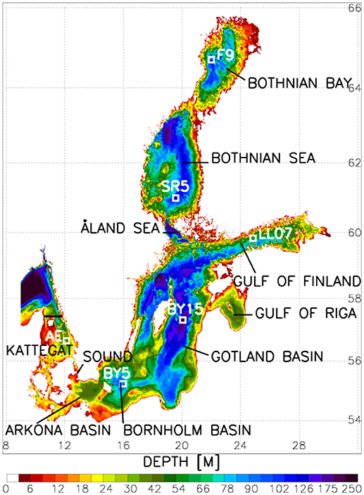
Figure 1. Bottom topography of the Baltic Sea and locations of the monitoring stations Anholt East in Kattegat (AE), Bornholm Deep (BY5), Gotland Deep (BY15), LL07 in the Gulf of Finland, SR5 in the Bothnian Sea and F9 in the Bothnian Bay. The Baltic proper comprises the Arkona Basin, Bornholm Basin and Gotland Basin.
In the Baltic Sea, patterns of species diversity are controlled by freshwater supply from the large catchment area and salt water inflows from the North Sea (Remane and Schlieper, 1971). Large landscape and land use gradients are found also over the Baltic Sea drainage basin, from densely populated southern areas with its intensive agriculture to almost deserted northern rocks, forests and wetlands. Such unique combination of natural and socio-economic features determines strong geophysical, biogeochemical, and ecosystem gradients (Schneider et al., 2017; Snoeijs-Leijonmalm and Andrén, 2017) that are very challenging to numerical modeling, especially to simulations involving scenarios of both climate (e.g., temperature and precipitation) and anthropogenic (e.g., nutrient inputs) changes (e.g., Vuorinen et al., 2015; Meier et al., 2018b).
To project future changes of the Baltic Sea scenario simulations have been developed during the past decade using coupled physical-biogeochemical models of varying complexity (BACC Author Team, 2008; BACC II Author Team, 2015). From recent transient scenario simulations for the period 1960–2100 it was found that water temperatures will increase and sea-ice cover will decrease in the future (BACC II Author Team, 2015). For instance, Meier (2006) calculated between the periods 1961–1990 and 2071–2100 an increase in volume averaged temperature between 1.9 and 3.2°C with an ensemble mean change of 2.5°C and a decline in sea-ice extent between 46 and 77% with an ensemble mean reduction of 62%. According to the BACC II Author Team (2015) salinity is projected to decrease due to the increased total annual river discharge. Future projections suggest that during winter runoff from the northern parts of the Baltic Sea catchment area will increase while during summer the runoff from the southern regions will decrease. From the overall increased total annual runoff, for instance Meier (2006) calculated a decrease in volume averaged salinity between 0.6 and 4.2 g kg−1 with an ensemble mean reduction of 2.3 g kg−1. Although in general wind changes over the Baltic Sea are small (Kjellström et al., 2011; Nikulin et al., 2011), higher wind speeds can be expected in regions where the sea-ice is projected to disappear on average affecting, e.g., currents, wind waves and resuspension (Eilola et al., 2013). However, sea level rise has a greater potential to increase surge levels than projected wind speed changes (Gräwe and Burchard, 2012).
The intensity and frequency of salt water inflows are projected to remain unchanged (Gräwe et al., 2013) or to slightly increase (Schimanke et al., 2014). However, in the latter study rising global mean sea level (GMSL) and changes in river runoff were not considered. Recent publications suggest that at least in sensitivity experiments exploring the impact of high-end projections following the Intergovernmental Panel on Climate Change (IPCC, 2007) GMSL rise will cause significant increases in (1) frequency and magnitude of salt water inflows (Hordoir et al., 2015; Arneborg, 2016), (2) salinity, and (3) phosphate concentrations in the Baltic Sea as a consequence of increased cross sections in the Danish straits, and will contribute to (4) increased hypoxia and anoxia (Meier et al., 2017). In these simulations, the increased phosphate concentrations in the water column originate from the fluxes between water column and sediment.
According to the BACC II Author Team (2015) climate change is likely to exacerbate eutrophication effects in the Baltic Sea because of (1) increased external nutrient loads due to increased runoff, (2) reduced oxygen flux from the atmosphere to the ocean, and (3) intensified internal nutrient cycling due to increased water temperatures (e.g., Meier et al., 2011, 2012a; Neumann et al., 2012; Omstedt et al., 2012). In the Baltic proper, higher water temperatures lead to faster phytoplankton growth and increased remineralization rates causing not only intensified nutrient cycling in the euphotic zone but also enhanced nutrient flows from the sediments due to a reduction in the nutrient retention capacity of the sediments (Meier et al., 2012b) caused by increased bacterial activity (e.g., Wulff et al., 2001). However, in the northern Baltic Sea phytoplankton production may actually be reduced in future climate due to increased allochthonous organic matter (Andersson et al., 2015).
Nutrient loads from land may vary differently than the volume flow due to changing soil moisture and soil temperature in future climate. Arheimer et al. (2012) found decreasing total nitrogen (N) and increasing total phosphorus (P) loads. According to their analysis, warmer temperatures may reinforce both denitrification causing N removal from the storage in water compartments and remineralization causing P accumulation in the water flow toward the sea.
Whether primary production and hypoxic area will increase in future climate will depend to a large extent on the nutrient load and greenhouse gas (GHG) emission or concentration scenarios (Meier et al., 2011; Saraiva et al., 2018). Future climate change will amplify oxygen depletion. Its impact on biogeochemical cycles is greater in the case of higher rather than lower nutrient loads. However, it has to be considered that the response of nutrient pools in the Baltic Sea to nutrient load changes will take several decades (Savchuk, 2018; and references therein).
In regions, such as the Bothnian Sea and the western Gulf of Finland, that may become on average ice-free in future climate, phytoplankton in spring will start growing earlier as a consequence of the shrinking sea-ice cover and improved light conditions and will decrease earlier due to earlier nutrient depletion (Eilola et al., 2013; their Figure 2F).
Neumann et al. (2012) suggested that also cyanobacteria blooms in the Baltic proper might occur earlier in summer. Such projected extension of the growth season and changes of the seasonal phytoplankton dynamics have already been detected in long-term satellite measurements (Kahru et al., 2016). Similar changes in seasonal dynamics of the surface water temperature are also reconstructed from field observations in all the major Baltic Sea basins but the corresponding changes in nutrient dynamics are not evident (Savchuk, 2018).
Concerning acidification the BACC II Author Team (2015) concluded that the rising atmospheric CO2 mainly controls future pH changes in Baltic Sea surface water and that eutrophication and enhanced biological production are not affecting the annual mean pH, but may amplify the seasonal cycle by increased production and remineralization (Omstedt et al., 2012). Depending on the CO2 emission scenario the pH of Baltic sea water will likely decrease further in the future.
The Baltic Sea is surrounded by nine riparian countries and therefore success of environmental management depends on concerted efforts of these countries. To facilitate this, all countries and the European Union (EU) have agreed to cooperate under the statutes of the Helsinki Convention and the implementation of the convention is coordinated by the Helsinki Commission (HELCOM). In addition, eight of the countries are EU member states and need to implement the Marine Strategy Framework and Water Framework directives (cf. Tedesco et al., 2016). A major step forward in the marine management was taken when the HELCOM Baltic Sea Action Plan (BSAP) was agreed by the HELCOM Contracting Parties in 2007 (HELCOM, 2007a,b) including concrete steps toward improved environmental status. One of the main components of the BSAP is a quantitative nutrient reduction scheme based on the ecosystem approach to management, providing reduction requirements per country and sub-basin, so called Country Allocated Nutrient Reduction Targets (CART) that should be achieved in order to mitigate eutrophication effects for the Baltic Sea. The reduction requirements were revised in 2013 based on new information (HELCOM, 2013a,b). The BSAP nutrient reduction scheme is based on the following steps (HELCOM, 2007a,b): (1) The politically agreed environmental objectives are translated into quantitative targets on observable variables in the sea (Secchi depth, Chl-a concentration, nutrient concentrations, oxygen deficit), (2) a biogeochemical model is used to estimate the maximum inputs per major sub-basin (so called Maximum Allowable Inputs, MAI) that will eventually lead to the achievement of target levels, and (3) the responsibility to perform the reduction necessary to achieve MAI for each sub-basin is shared between the countries (CART).
The assumptions how the MAI is implemented differ among the available scenario simulations. In some studies it was assumed that the nutrient loads after the year 2021 follow precisely the MAI (Friedland et al., 2012; Saraiva et al., 2018), whereas in other studies the impact of changing climate on the nutrient loads caused by the increased runoff and changes in other land surface processes is considered (Meier et al., 2011, 2012a; Neumann et al., 2012; BACC II Author Team, 2015).
In this pilot study, we assess the quality of available, state-of-the-art scenario simulations during the historical period 1980–2005 with the aim to reduce uncertainties and to raise confidence in projections of biogeochemical cycles. Henceforth, uncertainty is defined as the spread in future projections within an ensemble of scenario simulations expressed by the standard deviation of mean changes. Following climate modelers' terminology, we differentiate between scenario simulations (numerical model calculations based upon given assumptions) and scenarios (assumptions on nutrient load or radiative forcing that are not part of the applied model). We focus on the comparison between reference conditions from the recent past (1980–2005) and two nutrient load scenarios (REF and BSAP) for future climates (2072–2097). The REF scenario assumes unchanged reference conditions from the past also for future conditions.
From the analysis of the scenario simulations, we would like to answer the question whether current nutrient load abatement strategies, such as the BSAP (HELCOM, 2007a,b, 2013a,b) will meet their objectives of restored water quality status despite changing climate taking the uncertainties of the projections into account. For this aim, we analyzed results of scenario simulations performed in a number of international projects, such as ABNORMAL (Skogen et al., 2014), AMBER (Vuorinen et al., 2015), ECOSUPPORT (Meier et al., 2014), INFLOW (Kotilainen et al., 2014), Baltic-C (Omstedt et al., 2014b) and BONUS BalticAPP (Saraiva et al., 2018; Saraiva et al., submitted).
The nutrient load scenarios, REF and BSAP, correspond only to two out of five available Shared Socioeconomic Pathways (SSPs, O'Neill et al., 2014), i.e., SSP2 and SSP1, respectively (Zandersen et al., submitted manuscript) and do not represent the actual range of uncertainty. However, as we only focus on the question whether the BSAP will work in future climate taking plausible climate projections into account, nutrient load scenarios representing the other SSPs are not investigated. For comparison, only SSP2 (here defined as REF) is used as a business-as-usual scenario.
In an attempt to reduce uncertainties, we weighted the various scenario simulations with respect to the quality of simulated temperature, salinity and dissolved inorganic nitrogen, phosphorus and oxygen concentrations during the historical period (1980–2005) using available data of the national, long-term environmental monitoring programs in all Baltic Sea countries and using various metrics. Hence, we studied the future changes and its spreads of the whole ensemble and of a subset of scenario simulations with by definition “acceptable” quality to investigate whether the results of the projections depend on the quality of the models. In this approach, the definition and the assessment of the quality of the models are based on the evaluation of a cost function penalizing annual and seasonal mean biases normalized with the standard deviations of observations (e.g., Eilola et al., 2011; Skogen et al., 2014; Edman et al., 2018).
The paper is organized as follows. In section Methods, the involved global and regional climate models, the Baltic Sea models, the nutrient load and GHG emission scenarios, the list of investigated scenario simulations and the method of weighting the ensemble are introduced. In section Results, results of selected scenario simulations and of ensembles of weighted and unweighted scenario simulations are presented. In section Discussion, the advantages and disadvantages of weighting are discussed. In section Conclusions, some conclusions of the study are drawn.
We collected data from scenario simulations of six coupled physical-biogeochemical Baltic Sea Models (BSMs, see Table 1) driven by eight climate models (Table 2). Each climate model consists of a global General Circulation Model (GCM) or ESM (Earth System Model including also the carbon cycle), a regional climate atmosphere or atmosphere-ocean model (RCM), a land surface model (LSM) and one or two GHG emission scenarios. From all models, we defined eight subsets, each consisting of a combination of one BSM and one LSM. Henceforth, these subsets are called Baltic Region Models (BRMs) or Model A to H (Table 2). For each BRM the ensemble means of all scenario simulations were calculated for REF and BSAP nutrient load scenarios. The hierarchy of models used to carry out the scenario simulations is summarized in Figure 2.
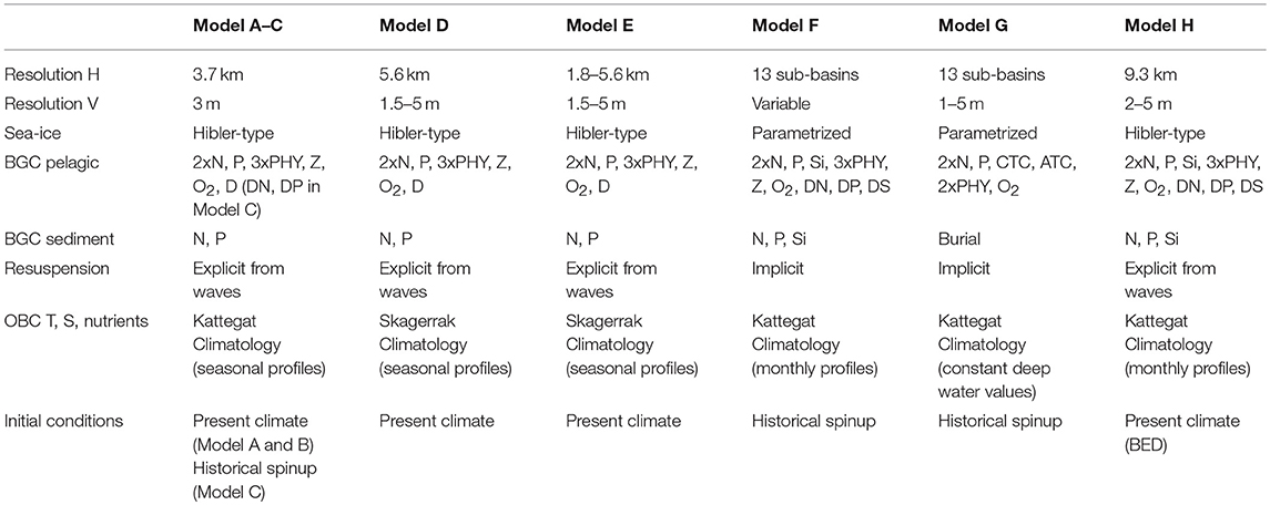
Table 1. Baltic Sea models (N, nitrogen; P, phosphorus; Si, silica; CTC, total inorganic carbon; ATC, total alkalinity; PHY, phytoplankton; O2, oxygen (or hydrogen sulfide); D, dead organic matter; Z, zooplankton; H, horizontal; V, vertical; BGC, biogeochemical cycling; OBC, open boundary conditions; T, temperature; S, salinity; BED, Baltic Environmental Database).
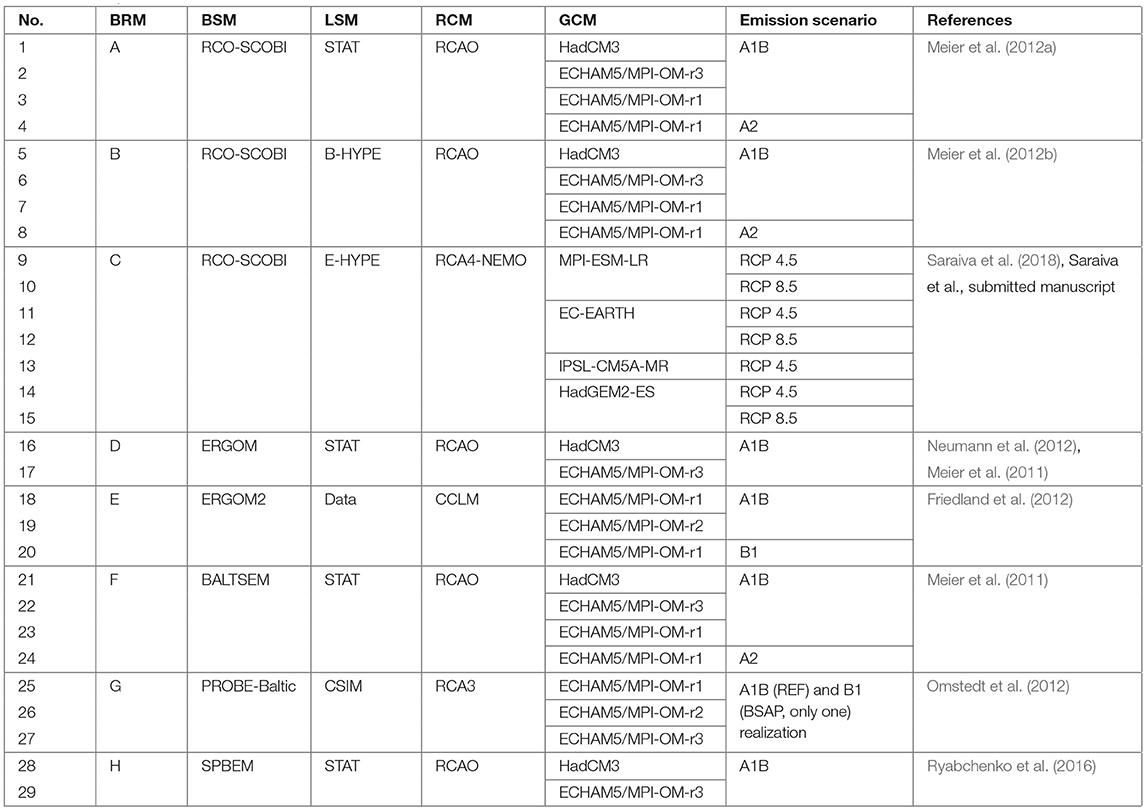
Table 2. List of scenario simulations (BRM, Baltic Region Model; BSM, Baltic Sea Model; LSM, land surface model; RCM, regional climate model; GCM, global general circulation model).
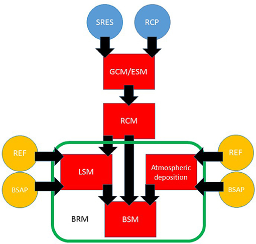
Figure 2. Model hierarchy consisting of a global General Circulation Model (GCM) or Earth System Model (ESM), a Regional Climate Model (RCM), a Land Surface Model (LSM), a Baltic Sea Model (BSM) and scenarios for radiative forcing according to Representative Concentration Pathways (RCPs) or the Special Report on Emission Scenarios (SRES) and nutrient loads (Reference–REF and Baltic Sea Action Plan–BSAP). A Baltic Region Model (BRM) comprises one BSM and one LSM. For details see text.
The projections are based on regionalized GCM results of the third and fourth assessment reports of the (IPCC, 2007, 2013) based on the Coupled Model Intercomparison Projects, CMIP3 and CMIP5, respectively. Regionalized model data from both CMIPs were analyzed together because otherwise the size of our ensemble would be too small. Knutti and Sedláček (2013) showed that the projected changes in the global patterns of air temperature and precipitation between CMIP3 and CMIP5 are remarkably similar and that the local model spread has not changed much motivating our approach to analyze both sets of scenario simulations together. Two GCMs from CMIP3, i.e., ECHAM5/MPI-OM (Jungclaus et al., 2006; Roeckner et al., 2006) and HadCM3 (Gordon et al., 2000), were used. For ECHAM5/MPI-OM three realizations (ECHAM5/MPI-OM-r1, -r2, -r3) based on the same model version but with differing initial conditions were available to study the impact of natural variability on the projections (e.g., Meier et al., 2012a). From CMIP5 four ESMs were used: MPI-ESM-LR (Block and Mauritsen, 2013; Stevens et al., 2013; https://www.mpimet.mpg.de), EC-EARTH (Hazeleger et al., 2012; https://www.knmi.nl), IPSL-CM5A-MR (Marti et al., 2010; Hourdin et al., 2013; http://icmc.ipsl.fr/) and HadGEM2-ES (Jones et al., 2011; http://www.metoffice.gov.uk). For the dynamical downscaling two uncoupled RCMs (CCLM, Rockel et al., 2008; RCA3, Samuelsson et al., 2011) and two coupled RCMs (RCAO, Döscher et al., 2002; RCA4-NEMO, Gröger et al., 2015; Wang et al., 2015) were applied.
For climate studies in the Baltic Sea region, BSMs and LSMs of varying complexity are applied (BACC II Author Team, 2015). BSMs are either (1) process-oriented, spatially integrated (e.g., Omstedt, 2015) or (2) three-dimensional, spatially resolved ocean circulation models (e.g., Griffies, 2004). From precipitation and air temperature LSMs calculate river runoff and river-borne nutrient loads from land to sea. LSMs are statistical models with simple assumptions on related nutrient loads (e.g., Meier et al., 2012a) or process-based models that consider biogeochemical cycles in vegetation and soils (e.g., Arheimer et al., 2012). In the following, the eight BRMs of this study are introduced (see also Tables 1, 2).
Model A to C: The Rossby Centre Ocean model (RCO) is a Bryan-Cox-Semtner primitive equation circulation model coupled to a Hibler-type sea-ice model with elastic-viscous-plastic rheology and open boundary conditions in the northern Kattegat (Meier et al., 2003). RCO is coupled to the Swedish Coastal and Ocean BIogeochemical model (SCOBI) describing nitrogen and phosphorus cycling in the water and sediment (Eilola et al., 2009). Boundary conditions at the sea floor are provided by a simple, vertically integrated sediment module. With the help of a simplified wave model, the combined effect of waves and current induced shear stress is considered to calculate resuspension of organic matter (Almroth-Rosell et al., 2011). The horizontal and vertical resolutions of RCO-SCOBI are about 3.7 km and 3 m, respectively. RCO-SCOBI was driven with (1) a statistical model for runoff and nutrient loads (STAT) and CMIP3 forcing (Model A, Meier et al., 2012a) and two versions of a process-based LSM, i.e., (2) B-HYPE (Arheimer et al., 2012) and CMIP3 forcing (Model B, Meier et al., 2012b), and (3) E-HYPE (Donnelly et al., 2013, 2014, 2017; Hundecha et al., 2016) and CMIP5 forcing (Model C, Saraiva et al., submitted).
Model D and E: The Ecological ReGional Ocean Model (ERGOM, see www.ergom.net) is a marine biogeochemical model coupled with an ocean general circulation model and a Hibler-type sea-ice model (MOM, Griffies, 2004). ERGOM describes the pelagic and benthic cycling of nitrogen and phosphorus with emphasis on changing redox conditions. Boundary conditions at the sea floor are provided by a simple, vertically integrated sediment module. With the help of a simplified wave model, resuspension of organic matter is calculated. The horizontal resolution of the model is about 5.6 km; the vertical resolution is 1.5 m in the upper 30 m and below that depth gradually increasing up to 5 m (Eilola et al., 2011; Neumann et al., 2012). A second model setup based on ERGOM was used (“ERGOM 2”), which has a finer horizontal resolution of 1.8 km in the southwestern Baltic Sea and 5.6 km elsewhere with a transition zone in between (Friedland et al., 2012; Schernewski et al., 2015). ERGOM and ERGOM2 were driven by the hydrological model STAT and by observed river runoff and nutrient loads from the end of the twentieth century, respectively. Both models are driven by CMIP3 regionalizations.
Model F: BALTSEM (BAltic sea Long-Term large-Scale Eutrophication Model; Savchuk, 2002; Gustafsson, 2003; Gustafsson et al., 2012; Savchuk et al., 2012) resolves the Baltic Sea spatially in 13 dynamically interconnected and horizontally averaged sub-basins with high vertical resolution, albeit morphometrically different from PROBE (see below). BALTSEM has a dynamical sea-ice model for leads (Nohr et al., 2009). Simulations were done using the NP version of the model, which describes nitrogen, phosphorus and silica cycles driven by water transports and biogeochemical fluxes. The sediment module is similar to the one used by Model C based on Savchuk (2002). Oxygen is a prognostic variable coupled to the production and remineralization of organic matter. BALTSEM scenario simulations were driven by STAT and CMIP3 forcing.
Model G: The PROBE-Baltic model is a fully coupled physical-biogeochemical model that resolves the Baltic Sea into 13 sub-basins with natural boundaries following the ecosystem-based regions and with high vertical and temporal resolutions for each sub-basin (Omstedt, 2015). The coupling of sub-basins is ensured through simplified strait flow models. The one-dimensional sea-ice model is based upon Omstedt and Nyberg (1996). The PROBE-Model system includes the carbon, nitrogen and phosphorus dynamics under both oxic and anoxic conditions (Edman and Omstedt, 2013). PROBE scenario simulations were driven by the Catchment Simulation Model, CSIM (Mörth et al., 2007; Omstedt et al., 2012), and CMIP3 forcing.
Model H: The St. Petersburg Baltic Eutrophication Model (SPBEM) is a coupled three-dimensional eco-hydrodynamic model with a modular structure. The hydrodynamic module of the model consists of models simulating the circulation patterns of the sea and sea-ice (Neelov et al., 2003; Myrberg et al., 2010). The biogeochemical module consists of pelagic and benthic models that are largely similar to BALTSEM (e.g., Savchuk, 2002). The horizontal resolution of the implemented version of SPBEM is 9.3 km; the vertical resolution is 2 m in the upper 100 m and 5 m in the lower layers (Ryabchenko et al., 2016). SPBEM scenario simulations were driven by STAT and CMIP3 forcing.
All BSMs except PROBE-Baltic are also described and compared by Tedesco et al. (2016).
The nutrient loads of the two scenarios, REF and BSAP, differ considerably among the models both during historical and future periods, in particular for phosphorus (Figure 3). These differences are explained by differing assumptions on bioavailable fractions of nutrient loadings from land (Eilola et al., 2011). However, even for the same BSM the nutrient loads vary because of differing LSMs with differing historical loads and climate sensitivities. For instance, in Model C phosphorus loads are 24% larger than in Model A during the historical period. Under the REF scenario both increasing and decreasing nutrient loads in future climate compared to the historical period are applied. In all models the BSAP scenario is characterized by lower nutrient loads compared to the historical period although the relative changes between future and historical periods differ. In some scenario simulations it is assumed that the BSAP is implemented as planned whereas in other LSMs the effects of increased runoff and changing soil processes in future climate are considered, counteracting the reduction in riverine nutrient concentrations (Meier et al., 2011). For instance, in Model A and C phosphorus loads are reduced in the BSAP scenario by 24 and 61% in the future compared to the historical period, respectively. The differences between the changes in nitrogen loads in Model A and C are smaller and the changes amount to 26 and 30%, respectively. Corresponding scenarios for the atmospheric nitrogen and phosphorus deposition are used (Figure 3).
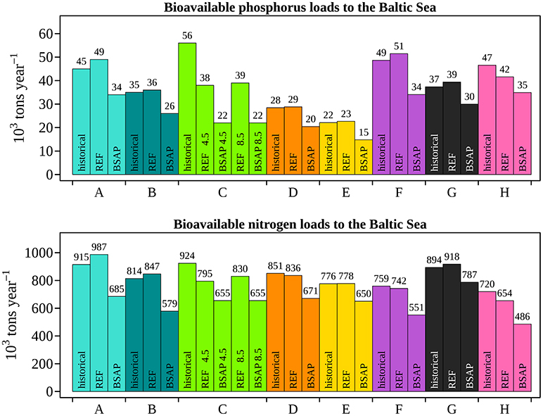
Figure 3. Projected ensemble means of total (land and atmosphere) bioavailable annual nutrient loads (phosphorus–upper panel, nitrogen–lower panel) to the Baltic Sea in historical (1980–2005) and future (2072–2097) climates for the scenarios REF and BSAP. At the x-axis the scenario simulations of Model A to H are listed (with a color code as in the other figures of this study). Note that for Model C projections driven by both RCP 4.5 and RCP 8.5 are shown. Model A (RCO-SCOBI coupled to STAT), B (RCO-SCOBI coupled to B-HYPE), C (RCO-SCOBI coupled to E-HYPE), D (ERGOM coupled to STAT), E (ERGOM2 using data), F (BALTSEM coupled to STAT), G (PROBE-Baltic coupled to CSIM), and H (SPBEM coupled to STAT).
The GHG emission scenarios differ among the scenario simulations. The concept of the GHG emission scenarios changed between CMIP3 and CMIP5. Whereas, in CMIP3 GHG emission scenarios by Nakicenovic et al. (2000), such as A1B, A2 and B1 were applied, the emissions in CMIP5 were based on Representative Concentration Pathways (RCPs) corresponding to a radiative forcing at the end of the century of 4.5 and 8.5 Wm−2, respectively (Moss et al., 2010). For instance, the difference in global temperature change between A1B and A2 are significantly smaller than between RCP 4.5 and RCP 8.5 (Rogelj et al., 2012; their Figure 3). As the results of ECHAM5/MPI-OM A1B and A2 are rather similar we used just one ensemble for Model A, B, and F following Meier et al. (2011). For Model E and C we combined scenario simulations under A1B and B1 and RCP 4.5 and RCP 8.5, respectively. The impact on nutrient loads in Model C under RCP 4.5 and RCP 8.5 is illustrated in Figure 3. Hence, the ensemble mean changes of these models follow a mean GHG emission scenario. In case of Model G, we followed the strategy of the original study by Omstedt et al. (2012). Thus, the REF and BSAP nutrient load scenarios were combined with A1B and B1 GHG emission scenarios, respectively.
The 58 scenario simulations from various projects collected for this study (Table 2) were not coordinated. Hence, the setups of the simulations, such as initial and lateral boundary conditions, nutrient loads and bioavailable fractions differ (Table 1; Figure 3) and a model intercomparison is impossible. For the latter, model simulations with the same external forcing, initial conditions and internally used datasets, such as the bathymetry would be required (cf. Placke et al., 2018; this research topic).
All scenario simulations are transient runs that start in the time interval 1958–1975 and terminate at the end of the twenty-first century. In case of the Model C and F a spinup was performed using reconstructed atmospheric, hydrological and nutrient load forcing since 1850 (Gustafsson et al., 2012; Meier et al., 2012c, 2018b; Schenk and Zorita, 2012). In case of Model G, even a long-term spinup since 1500 was performed (Hansson and Gustafsson, 2011). In all models at the lateral boundaries in Kattegat or Skagerrak climatological observations with differing resolution were prescribed or nudged throughout the entire simulation. In 1975 (Model C), 1961 (Model F) or 1958 (Model G) the atmospheric forcing switched from reconstructed to climate model data. Henceforth, the simulations during the historical period are called control simulations.
All projections were published in peer-reviewed literature and are a priori regarded as equally plausible. Nevertheless, in the assessment of this study the performance of the various control simulations was evaluated to investigate whether the quality of the control simulations and the spread of the projections are connected. The assessment was done both for each of the 29 control simulations and for the eight BRMs. The latter approach (clustering by BRMs) assumes that the largest uncertainty in biogeochemical cycling during the control period originates from process descriptions in the Baltic Sea and from the runoff and nutrient loads from land. The clustering of scenario simulations by BRMs was performed for clarity of the presentation but does not influence the main conclusions of this study. As most of the earlier studies considered at least the ensemble mean and a high-end climate scenario, the impact of climate change is considered in all BRM simulations approximately in the same way. However, we are aware that scenario simulations of the third and fourth assessment reports of the (IPCC, 2007, 2013) differ. For instance, the warming of the A1B emission scenario is in between the corresponding air temperature changes in RCP 4.5 and RCP 8.5 scenarios (Knutti and Sedláček, 2013). Nevertheless, authors of previous studies have used both A1B and RCP 4.5 as representatives of the ensemble mean (e.g., Meier et al., 2012a; Saraiva et al., 2018). Hence, we consider this choice as part of the uncertainty in Baltic Sea projections. Sources of uncertainties are not investigated here and will be studied separately.
For the model evaluation observed and simulated annual and seasonal mean profiles of temperature, salinity and oxygen, ammonium, nitrate and phosphate concentrations at the monitoring stations Anholt East (AE), Bornholm Deep (BY5), Gotland Deep (BY15), Gulf of Finland (LL07), Bothnian Sea (SR5), and Bothnian Bay (F9) were compared (Figure 1). The inter-annual variability of the simulated variables was not assessed. The mean profiles were calculated for the historical period. In this study, post-processed data from the Baltic Environmental Database (BED) were used (Gustafsson and Rodriguez Medina, 2011). Data are available every 5 m near the surface, every 10 m between 20 and 100 m depth, and for stations reaching even deeper data are predominantly available every 25 m. At these standard depths, observations are gathered from a depth range of one meter above and one meter below the standard depth.
In this study, the model-data comparison is restricted to abiotic natural prototypes that are rather unequivocally represented in the models. In contrast to some other formulations (e.g., Baird et al., 2013; Vichi et al., 2015; Butenschön et al., 2016), none of our models explicitly simulates the chlorophyll cell quota as a separate model variable. Meanwhile, the stoichiometric ratio between chlorophyll and other characteristics of phytoplankton biomass varies both between and within algae species in dependence on ambient environment and the recent history of populations, for instance, in the range from 20 to 100 (g C:g Chl-a) as a conservative estimate (e.g., Wasmund and Siegel, 2008; Spilling et al., 2014; Jakobsen and Markager, 2016). Within the large meridional and phenological Baltic Sea gradients, the usage of fixed conversion from biomass simulated in nitrogen or carbon units to chlorophyll concentration would introduce an unknown inherent uncertainty, thus unnecessarily compromising judgement of the model's plausibility. In addition, the models represent horizontally and vertically averaged values (of different degree depending on grid sizes) while observations are pointwise and may be affected by small-scale patchiness, which may be especially pronounced for the biological components.
Two skill metrics were combined to define a cost function for the control simulations. The vertical and seasonal mean bias, C > 0, is the average of all i = 1, …, n absolute differences between model, Pi, and observation, Oi, averages at each depth and time of the year divided by the standard deviation, σ, of the observations.
The Pearson correlation coefficient, R > 0, measures the similarity in the shape of the mean profiles, i.e., how well the simulated and observed vertical mean profiles and seasonal cycles agree.
We tested various differing normalized cost functions, CQ, such as
based on annual and seasonal means. If R = 1 (perfect agreement in the shape of the profiles or seasonal cycle), a mean bias of the model results smaller than two standard deviations of the observations, which is regarded as an acceptable quality according to Eilola et al. (2011), would result in a cost function CQ < 1. If C = 0 (no mean bias), a correlation coefficient of R > 1/3 would result in CQ < 1. For most variables and for all investigated monitoring stations the annual mean bias is a more restrictive skill metric than the correlation coefficient (not shown). As the outcomes for CQ do not differ much regardless of the choice of the metric, in this study the following cost function based on annual mean variables was used:
For C < 2 or CQ < 1, the quality was regarded as acceptable (Eilola et al., 2011). Thus, per definition model results are acceptable when the mean biases during the control period are less than two standard deviations of the observations on average. This criterion was defined as the threshold for a model simulation to be included in the weighted ensemble. Members of the ensemble with CQ > 1 were disregarded. From the cost functions weights, Wjkl, for each control simulation j per station k and variable l were calculated according to
Finally, for each run of Model A to H one cost function and one weight is calculated by averaging all cost functions of all stations and variables. The calculation of the combined cost functions and combined weights is done without the monitoring station Anholt East (AE) because for some of the BSMs this station is located near the model's lateral boundary.
In the following, we discuss results of the weighted and unweighted ensemble means at Gotland Deep compared to annual or winter mean observations (Figure 4). After 1990, annual mean sea surface temperature (SST) observations are usually within one standard deviation of the climate model results, which is regarded as good. Note that prior to 1990 the annual mean SST calculated from observations might be biased due to missing observations. This also applies to all other variables with a pronounced seasonal cycle. Sea surface salinity (SSS) is overestimated during the historical period by several models indicating problems with the representation of the pronounced vertical gradients in the Baltic Sea. Due to spurious numerical mixing the vertical salt flux might be too large (Rennau and Burchard, 2009). In two of the simulations, SSS amounts to 12–13 g kg−1 instead of 7 g kg−1 in observations whereas the other simulations are much closer to observations (not shown). The weighted ensemble means of simulated SSS are close to observations whereas unweighted ensemble means overestimate observations considerably. Also for deep water temperature and oxygen concentration slight differences between weighted and unweighted ensemble means are found. The weighted ensemble mean deep water is warmer and more oxygenated. For all other variables, the two ensemble figures are relatively close to each other. As the pronounced decadal variations in deep water temperature and salinity, deep water oxygen concentration and surface water phosphate concentration, such as the stagnation period during 1983–1993, cannot be reproduced by climate simulations, deviations between ensemble mean model results and observations are expected. Weighted and unweighted ensemble mean deep water salinities are close to observations. Finally, there is a tendency of under- and overestimated winter mean surface dissolved inorganic nitrogen (DIN, i.e., nitrate and ammonium) and phosphorus (DIP, i.e., phosphate) concentrations, respectively.
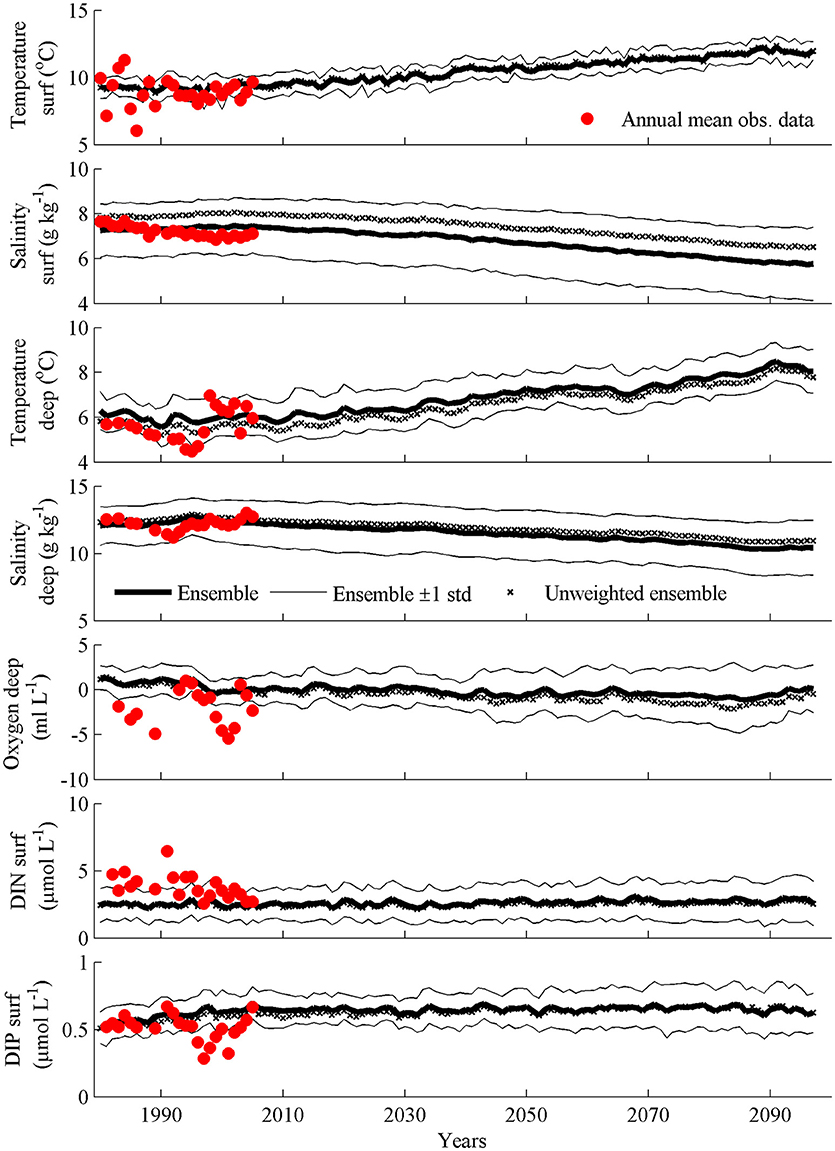
Figure 4. Simulated (black lines) and observed (red circles) annual mean water temperatures (in °C) and salinities (in g kg−1) at Gotland Deep in the surface (surf) and deep layer (deep), annual mean oxygen concentrations (in mL O2 L−1) in the deep layer, and winter (December-February) mean dissolved inorganic nitrogen (in mmol N m−3) and phosphorus (in mmol P m−3) concentrations in the surface layer. Data have been extracted from the models' top grid cell for the surface layer (surf) and for the grid cell closest to 200 m for the deep layer (deep). Shown are the weighted and unweighted ensemble means and plus/minus one standard deviations of all simulations performed with Model A to H for the period 1980–2097. In all scenario simulations, the REF nutrient load scenario is applied.
For most simulations and monitoring stations, the values of the normalized cost function (Equations 1, 4) are lower for temperature and higher for salinity and phosphate (Figure 5). Further, cost functions are smaller in the southwestern and higher in the northern Baltic Sea with some exceptions, such as salinity. These results indicate smaller mean biases of the historical model results for temperature relative to salinity and phosphate and a better model representation of the southern relative to the northern Baltic Sea in accordance to Eilola et al. (2011). The horizontal and vertical stratification in the Baltic Sea is dominated by salinity gradients, which are controlled by freshwater supply from rivers, salt water inflows from the Kattegat, intrusions into the Gotland Basin and mixing while temperature gradients are predominantly controlled by air-sea fluxes. The northern Baltic Sea (in particular the Bothnian Bay) is perhaps more difficult to simulate because of, inter alia, the seasonal sea-ice cover and seasonal vertical stratification, a P-limited environment, a more important microbial loop, and a larger CDOM contribution limiting light conditions (e.g., Andersson et al., 2015). Recently, Fransner et al. (2018) showed that non-Redfieldian dynamics explain the seasonal pCO2 cycle in the Bothnian Sea and Bothnian Bay. However, most biogeochemical models of the Baltic Sea are based on Redfield stoichiometry (e.g., Savchuk, 2002; Eilola et al., 2009; Neumann et al., 2012; Omstedt et al., 2012; Ryabchenko et al., 2016).
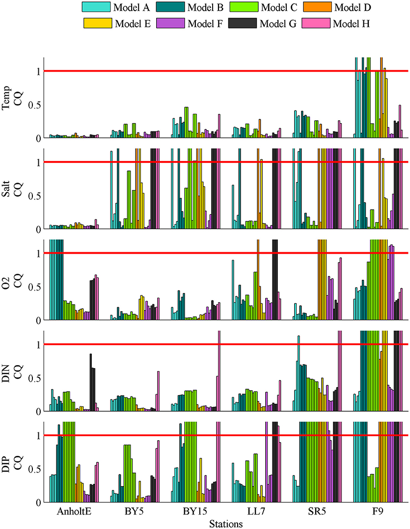
Figure 5. Normalized cost function (Equation 4) for temperature, salinity, oxygen, DIN and DIP concentrations at the monitoring stations Anholt East (AE), Bornholm Deep (BY5), Gotland Deep (BY15), Gulf of Finland (LL07), Bothnian Sea (SR5), and Bothnian Bay (F9) for all scenario simulations of Model A to H during the historical period 1980–2005. Only simulations with a cost function value, CQ, smaller than one (red line) for all stations and all variables are considered for the weighted ensemble.
If we neglect the station in Kattegat for the following discussion, oxygen concentrations are more accurately simulated in the Bornholm Basin and Gotland Basin than in the Gulf of Finland, Bothnian Sea and Bothnian Bay (Figure 5). In most sub-basins and most simulations, DIN concentrations are of acceptable quality except in the Bothnian Bay. In several simulations, phosphate concentrations in the Gotland Basin, Gulf of Finland, Bothnian Sea and Bothnian Bay are biased. However, the magnitude of the cost function varies considerably among the models.
An exception is the monitoring station Anholt East (AE) in Kattegat (Figure 5). The poor results of some control simulations at this station (Model A and B for oxygen and Model B and C for phosphate) might indicate problems of the corresponding setups at the lateral boundaries of the model domain.
No control simulation fulfills the criterion CQ < 1 (Equation 4, mean model bias smaller than two standard deviations of the observations on average) at all stations and for all variables and there is no unambiguously best or worst model. The cost functions (Figure 5) and related weights (Figure 6) vary substantially between the variables and stations. For all variables the number of simulations considered for the calculation of the weights are much smaller in the northern than in the southern Baltic Sea (Figure 6). For instance, in the Bornholm Basin all 29 control simulations perform acceptably for temperature, oxygen, DIN and DIP concentrations. A corresponding number of simulations for salinity is 20. However, for the same variables in the Bothnian Bay we found that only 18 (temperature), 19 (salinity), 16 (oxygen concentration), 10 (DIN concentration), and 7 (phosphate concentration) simulations are of acceptable quality. For phosphate in the Bothnian Bay the 7 acceptable simulations were performed with only one BRM (Model C).
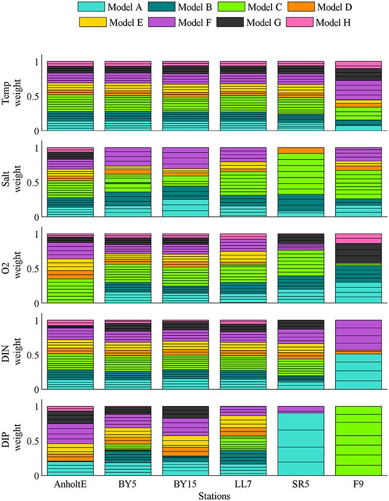
Figure 6. Weights (Equation 5) for each variable, station and scenario simulation of Model A to H.
When results of the simulations are weighted for each variable independently, ensemble mean results would be rather artificial because the weighted variables are not dynamically consistent anymore. In this case, the number of simulations contributing to the weights for each variable and station would be different (Figure 6). Hence, for each Model A to H we combined the weights for each simulation by calculating the averages over all stations, simulations and variables. Following this strategy the combined cost function with the criterion CQ < 1 suggests that 17 out of 29 scenario simulations are of acceptable quality (Figure 7). These simulations belong to four BRMs, i.e., Model A, B, C, and F, that are of acceptable quality. Indeed, the cost functions vary considerably between the simulations. Only two out of six BSMs dominate the sum of all weights and, consequently, the ensemble mean.
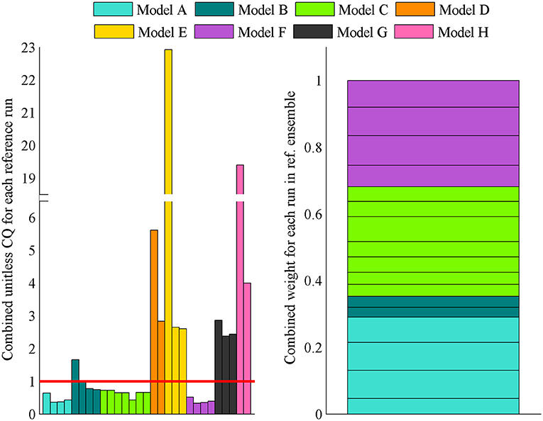
Figure 7. Combined cost function calculated from all variables and stations. Shown are the results for all 29 control simulation of Model A to H.
Figure 4 shows the ensemble mean and spread of all scenario simulations driven with various greenhouse gas emission and nutrient load scenarios at Gotland Deep to illustrate the wide range of the responses. In the unweighted and weighted ensembles projected changes at the end of the century are not necessarily larger than the biases during the historical period, i.e., the signal-to-noise ratio is relatively small (Figure 4). In particular, considerable differences between the means of weighted and unweighted model results for SSS are found. Nevertheless, both weighted and unweighted ensemble mean model results clearly show increased temperatures, decreased salinities, decreased deep water oxygen concentrations and increased surface water phosphate concentrations.
Figure 8 shows the weighted and unweighted ensemble mean changes between future and historical periods (including also various GHG emission scenarios) for the nutrient load scenarios REF and BSAP. Annual surface and bottom water temperatures increased by about 2–3 and 1–2°C in the weighted ensemble mean, respectively. Surface temperature changes are slightly larger in the northern than in the southern Baltic Sea because of the ice-albedo effect (Meier et al., 2012a). A contrary behavior was found for bottom temperatures with slightly smaller changes in the northern than in the southern Baltic Sea perhaps because of warm salt water inflows from Kattegat that only affect the Baltic proper and Gulf of Finland directly (Matthäus and Franck, 1992). Annual surface and bottom salinity changes amount to about −1 to −1.5 and −1 to −2 g kg−1, respectively. Salinity changes both at the surface and at the bottom are slightly smaller in the northern than in the southern Baltic Sea in accordance with results by Meier (2006) because salinity changes due to increased river runoff are smaller in case of smaller salinities (Meier and Kauker, 2003).
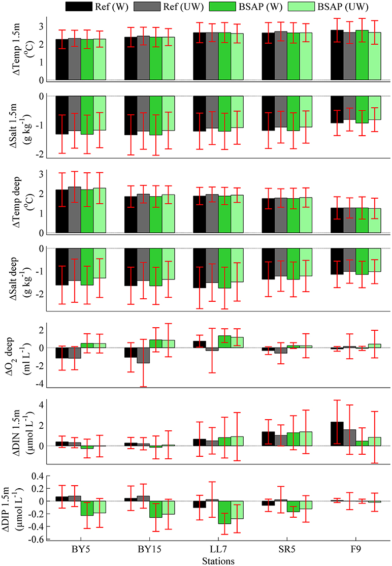
Figure 8. Weighted and unweighted ensemble mean changes and standard deviations (represented by error bars) in REF and BSAP scenario simulations for temperature, salinity, oxygen, dissolved inorganic nitrogen and phosphorus concentrations at the monitoring stations BY5, BY15, LL07, SR5 and F9 at 1.5 and 200 m depth. Data have been extracted from the models' top grid cell for the surface layer (1.5 m) and for the grid cell closest to 200 m or the deepest grid cell for the deep layer (deep). “W” and “UW” refer to weighted and unweighted ensemble mean results.
For annual mean deep water oxygen and winter mean surface nitrate and phosphate concentrations the weighted and unweighted ensemble mean changes depend on the nutrient load scenario (Figure 8). In both REF ensembles we found decreased deep water oxygen concentrations in the Baltic proper (at BY5 and BY15) perhaps reflecting (1) increased nutrient loads compared to the historical period in some of the projections (Figure 3), (2) increased temperature dependent stratification (Figures 9, 10), and (3) the impact of warming as explained by Meier et al. (2011). However, in the Gulf of Finland (at LL07) oxygen concentrations increase and decrease in the weighted and unweighted ensembles, respectively (for an explanation see below). In BSAP oxygen concentrations increase at all stations in both ensembles due to the decreased nutrient loads.
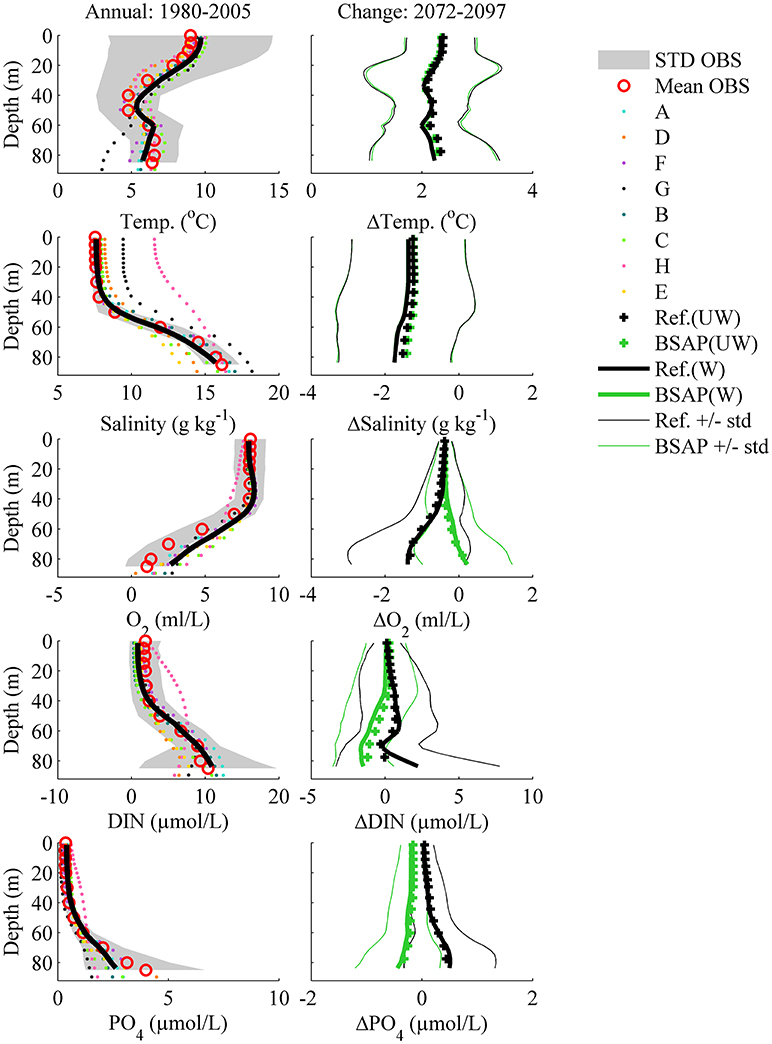
Figure 9. Mean observed and simulated profiles in the control runs for each variable and each Model A to H at Bornholm Deep (BY5) for the period 1980–2005 (left panels). The ensemble mean value (thick black line) is calculated from the weighted model results. In addition, the unweighted (plus signs) and weighted (thick solid lines) ensemble mean changes and standard deviations between the future (2072–2097) and present (1980–2005) climates in REF and BSAP scenario simulations are shown (right panels). Standard deviations are calculated from the two ensembles without weighting.
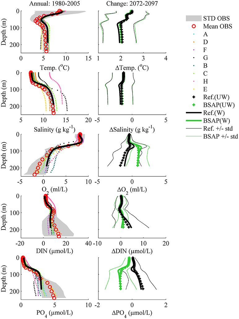
Figure 10. Mean observed and simulated profiles in the control runs for each variable and each Model A to H at Gotland Deep (BY15) for the period 1980–2005 (left panels). The ensemble mean value (thick black line) is calculated from the weighted model results. In addition, the unweighted (plus signs) and weighted (thick solid lines) ensemble mean changes and standard deviations between the future (2072–2097) and present (1980–2005) climates in REF and BSAP scenario simulations are shown (right panels). Standard deviations are calculated from the two ensembles without weighting.
There are slight increases in winter mean surface nitrate concentrations in both REF and BSAP except at BY5 and BY15 in case of BSAP in the weighted ensemble (Figure 8). In REF winter surface phosphate concentrations increase in the Baltic proper and decrease at LL07 and SR5 in the weighted ensemble. The latter decrease might be explained by smaller stratification and improved oxygen conditions in the deep water. Correspondingly, winter mean surface phosphate concentrations decrease at LL07 and SR5 in the unweighted ensemble following the changes in oxygen concentrations. In BSAP phosphate concentrations decrease at all stations in both ensembles. However, the changes at F9 are small. In summary, the changes in oxygen and phosphate concentrations qualitatively agree in the Baltic proper in the two ensembles but may differ in the northern Baltic Sea and Gulf of Finland with respect to their sign. However, the dominant impact of the BSAP on changes in biogeochemical variables compared to the changes in REF is clearly visible in both ensembles.
Further, the standard deviations of the changes of biogeochemical variables in simulations with an acceptable CQ are generally smaller than in the entire ensemble (Figure 8). Note, that the standard deviations of temperature and salinity changes in REF and BSAP are not identical because for Model G the REF ensemble consists of three simulations under the A1B scenario whereas the BSAP ensemble consists of only one simulation under the B1 scenario (Table 2).
The changes of profiles in the two ensembles of weighted and unweighted scenario simulations show some differences (Figures 9–13) but overall the responses to nutrient load changes in the Baltic proper (at BY5 and BY15, see Figure 1) are similar (Figures 9, 10). An exception is the northern Baltic Sea, in particular in the Gulf of Finland (station LL07, Figure 11) and Bothnian Bay (station F9, Figure 13), where we found larger differences between the two ensembles. The differences are relatively small for changes in temperature and salinity but larger for the biogeochemical variables (oxygen, DIN and DIP concentrations) in the deep water. Note that the spread of the changes in biogeochemical variables is larger in the deep water with larger oxygen variations than in the surface layer indicating an uncertainty in the fluxes between water column and sediment and between the surface and deep layer. For instance, in the unweighted ensemble the increase in mean oxygen concentration of the deep water at LL07 is by about 2 mL L−1 larger in BSAP than in REF whereas in the weighted ensemble the increase in oxygen concentration is much smaller. In the latter (weighted) ensemble, mean oxygen concentrations in both REF and BSAP are higher than in the unweighted ensemble with large impact on the simulated changes in biogeochemical cycles. In the Bothnian Sea (station SR5) the differences between weighted and unweighted ensembles are slightly larger than in the Baltic proper (Figure 12). Hence, weighting does not change the overall conclusion for the eutrophied Baltic proper (without the Gulf of Finland) whether the BSAP will work in future climates or not. However, in the northern Baltic Sea, such as the Bothnian Bay and the Gulf of Finland weighting matters.
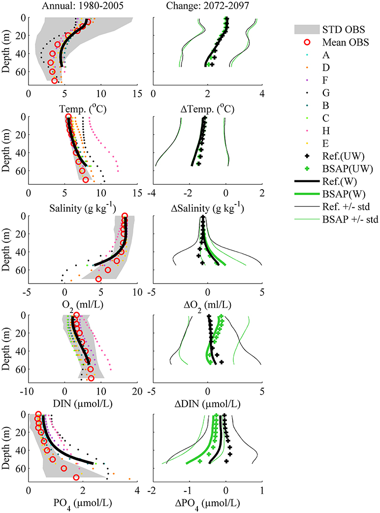
Figure 11. Mean observed and simulated profiles in the control runs for each variable and each Model A to H at LL07 in the Gulf of Finland for the period 1980–2005 (left panels). The ensemble mean value (thick black line) is calculated from the weighted model results. In addition, the unweighted (plus signs) and weighted (thick solid lines) ensemble mean changes and standard deviations between the future (2072–2097) and present (1980–2005) climates in REF and BSAP scenario simulations are shown (right panels). Standard deviations are calculated from the two ensembles without weighting.
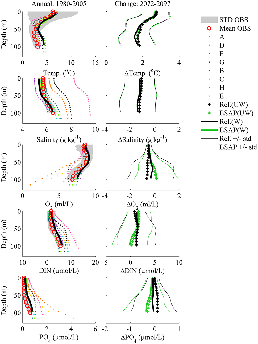
Figure 12. Mean observed and simulated profiles in the control runs for each variable and each Model A to H at SR5 in the Bothnian Sea for the period 1980–2005 (left panels). The ensemble mean value (thick black line) is calculated from the weighted model results. In addition, the unweighted (plus signs) and weighted (thick solid lines) ensemble mean changes and standard deviations between the future (2072–2097) and present (1980–2005) climates in REF and BSAP scenario simulations are shown (right panels). Standard deviations are calculated from the two ensembles without weighting.
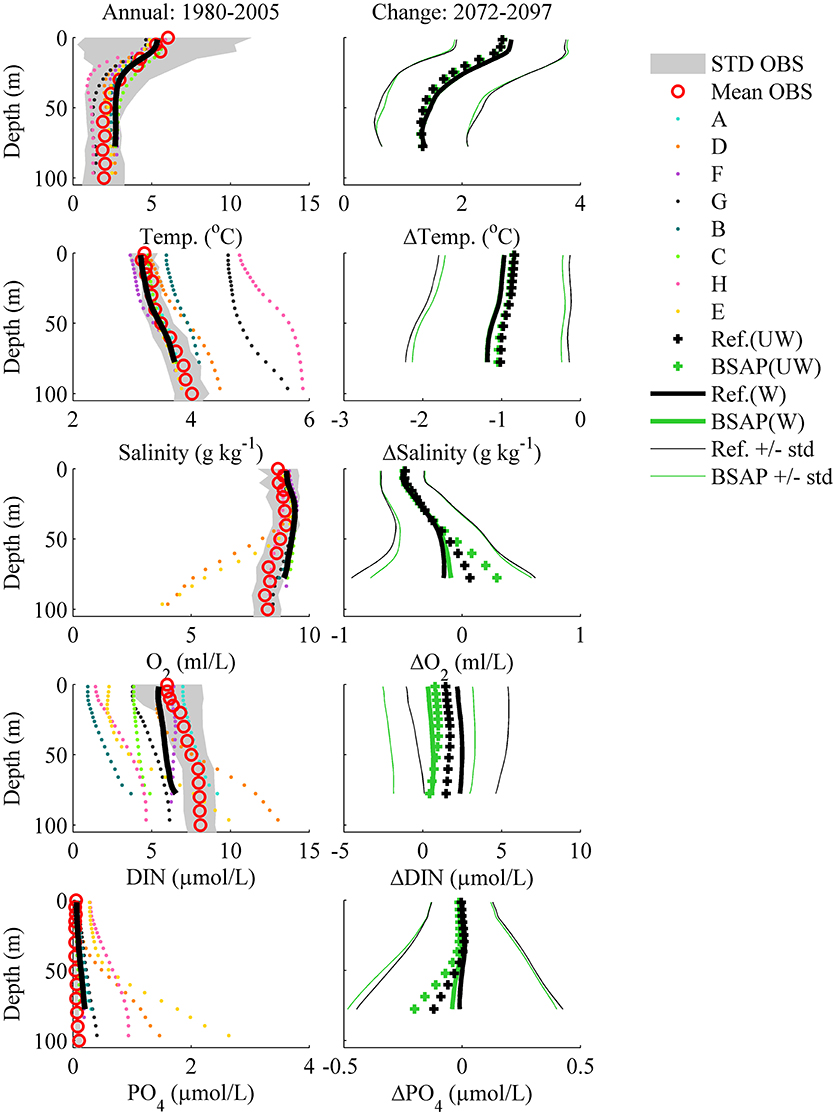
Figure 13. Mean observed and simulated profiles in the control runs for each variable and each Model A to H at F9 in the Bothnian Bay for the period 1980–2005 (left panels). The ensemble mean value (thick black line) is calculated from the weighted model results. In addition, the unweighted (plus signs) and weighted (thick solid lines) ensemble mean changes and standard deviations between the future (2072–2097) and present (1980–2005) climates in REF and BSAP scenario simulations are shown (right panels). Standard deviations are calculated from the two ensembles without weighting.
The weighting of model results from multi-model ensembles was investigated before (e.g., Christensen et al., 2010; Räisänen et al., 2010). The aim of weighting is to improve the estimates of climate change impacts and to reduce the ensemble spread by excluding (or giving lower weight to) ensemble members with insufficient performance in the control simulation of historical climate. Weighting assumes that there is a relationship between biases in historical climate and ensemble mean changes and their spread in future climate. Christensen et al. (2010) found that weighting adds another level of uncertainty to the generation of ensemble-based climate projections because the choice and combination of applied metrics is subjective. They concluded that there is no evidence of an improved description of mean climate states using weighted in comparison to unweighted ensembles. Räisänen et al. (2010) came to similar conclusions but found a not negligible decrease in cross-correlation error and that their method could potentially be improved.
In this study, we compared a large multi-model ensemble of scenario simulations with a subset of models with better performance than the entire ensemble. The simulated variables within the ensemble subset are dynamically consistent because we have not weighted the variables and stations independently but calculated a combined weight per simulation.
From this procedure, we may confirm the conclusions from the earlier studies. For the REF and BSAP scenarios the ensemble mean changes in future climate projections of these two ensembles are similar for the Baltic proper (Figures 9, 10) and Bothnian Sea (Figure 12). However, also in the sub-basins with larger discrepancies between weighted and unweighted ensembles the BSAP scenario will lead to an improved environmental status compared to REF despite the large spread in the ensembles. The results of the projections are robust with respect to the choice of the cost function or metric. However, we have only tested a limited number of metrics that measure the performance of the annual and seasonal mean states. For instance, an assessment of the frequency and intensity of extremes was not done.
The effect of weighting is to remove the impact from outlier models that do not perform well (either at stations or variables). As for many variables (except salinity and phosphate concentration), the model skills in the southern Baltic Sea are acceptable, differences between weighted and unweighted ensemble means are not expected (Figure 5). If the weighted and unweighted ensemble means in historical climate are close to each other, model errors will not be correlated and will compensate each other. On the other hand, stations and depths with large model biases indicate locations affected by physical or biogeochemical processes that are not well-understood or not well-resolved, such as steep slopes and large gradients in hydrography.
We also found that the ensemble mean changes in weighted and unweighted ensembles differ in the northern Baltic Sea, in particular in the Gulf of Finland (Figure 11). This might indicate that in the northern Baltic Sea the response of biogeochemical cycles to changing climate and changing nutrient loads depends more on the mean conditions during the historical period than in the southern Baltic Sea, i.e., the system response in the northern Baltic Sea is more non-linear than in the southern Baltic Sea. If the response to changing climate and changing nutrient loads is overwhelmingly non-linear, the differences between weighted and unweighted ensemble mean changes might be considerable.
The larger discrepancy between weighted and unweighted ensembles in the northern sub-basins might be caused by two reasons, i.e., (1) the ice-albedo feedback and (2) changes in river runoff. Ad (1): Due to the ice-albedo feedback small differences in the scenario simulations of the GCMs might cause large differences in the projected changes in sea-ice cover, warming of the water column, light conditions, resuspension, mixing, stratification, and primary production in the Baltic Sea (e.g., Eilola et al., 2013). Ad (2): In the Gulf of Finland, the sub-basin with the largest discrepancies between weighted and unweighted ensembles, increased freshwater supply will cause a weaker vertical stratification, improved oxygen conditions, changes in redox-dependent biogeochemical processes and water-sediment fluxes. The considerable spread in runoff projections (e.g., Meier et al., 2006, 2012b) may cause substantial differences in stratification and consequently in biogeochemical cycling due to changing redox conditions. For instance, the runoff changes between 2069–2098 and 1976–2005 calculated with the LSM E-HYPE driven by the regionalized ESMs MPI-ESM-LR, EC-EARTH, IPSL-CM5A-MR and HadGEM2-ES under the RCP 4.5 scenario amount to 1, 7, 21, and 14%, respectively (Saraiva et al., submitted). Corresponding figures for MPI-ESM-LR, EC-EARTH and HadGEM2-ES under RCP 8.5 are 15, 6, and 20%, respectively.
Further, the weighting method described here does not evaluate the climate sensitivity of the models. For such an evaluation much longer control simulations than those presented here for the period 1980–2005 including some trend analysis would be required driven by regionalized climate model data and evaluated with observations that do not exist. Our method may rank a model high, that may show an acceptable performance during the historical climate but may still have wrong climate sensitivity and, vice versa, a model with bad performance in present climate may work well in future climate. Our assumption that an acceptable performance during historical climate is a necessary condition for correct climate sensitivity cannot be verified.
It should be emphasized that this study is an assessment of existing scenario simulations and not an assessment of BSMs because the identified errors might originate from the dynamical downscaling approach including BSMs, LSMs, RCMs, and GCMs/ESMs. Recently, an assessment of hindcast simulations of ocean models was performed (Placke et al., 2018; this research topic). Assessments foster model development, inter alia, to improve scenario simulations. However, to reduce uncertainties in scenario simulations their sources (as discussed by Meier et al., submitted manuscript; this research topic) have to be identified and possibly removed.
For the estimation of uncertainties multi-model ensembles are needed. Due to limited computer resources, the number of climate projections is generally too small to access uncertainties adequately. Thus, an important question is how many members of an ensemble are really needed and whether an appropriately chosen sub-set of the ensemble may represent the uncertainty of the full ensemble (Wilcke and Bärring, 2016).
We have not addressed the differences in uncertainties between weighted and unweighted ensembles. However, a careful evaluation of all components of the model system may lead to a reduced number of ensemble members and to improved estimates of future projections. For the investigation of quality, we selected annual and seasonal mean variables. However, this choice does not guarantee more reliable climate sensitivity. To improve our approach we may evaluate also longer simulations including historical trends in eutrophication and changing climate constraining the long-term sensitivity of the models. So far, the climate sensitivity of the Baltic Sea has not been assessed thoroughly. However, recently historical reconstructions since 1850 became available that might be used, for instance together with light ship observations, for this purpose (Meier et al., 2012c, 2018a,b). However, such an evaluation of simulated past changes may not be sufficient for the evaluation of climate sensitivities that control the much larger changes in physical variables that are expected in future climate. Nevertheless, our assessment may contribute to improved credibility of scenario simulations.
In the present work eight differing BRMs applied in 58 transient scenario simulations representing modeling efforts in Sweden, Germany, Russia, Finland, Denmark, Poland and Estonia were assessed. This is the first time that such a large ensemble of different projections was investigated. From this study, we draw the following conclusions:
1. Differences between state-of-the-art scenario simulations for the Baltic Sea both during historical and future climates are considerable. Some models perform better than others in comparison to available monitoring data from 1980 to 2005.
2. In the eutrophied Baltic proper (excluding the Gulf of Finland) the ensemble mean changes in biogeochemical variables between REF and BSAP scenarios are similar between weighted and unweighted ensembles. Hence, weighting does not qualitatively affect ensemble mean changes. A relatively small number of models with acceptable quality compared to observations seems to be representative for the entire ensemble although more systematic research on this topic is needed. In the ensemble mean calculated from all unweighted simulations, model biases seem to compensate each other for most variables and locations. The results do not depend significantly on the choice of metric (for those that were tested).
3. Although uncertainties are large, we conclude that the rigorous implementation of the BSAP will result in improved environmental conditions despite the counteracting impact of changing climate. Hence, management questions can be answered despite considerable uncertainties.
4. Earth system modeling activities in the Baltic Sea region are intensive and of acceptable quality for some models. However, there is a strong need for regular assessments (like the pilot study presented here) that support (1) the modeling community with forcing and scenario data and with improved modeling tools and (2) marine management with improved best estimates of climate change impacts and their uncertainties.
Observations from the Baltic Environmental Database (BED) are publicly available from http://nest.su.se/bed. Model codes and data used for the analysis of this study are available from the authors upon request.
Conception and design of the assessment were discussed during two Baltic Earth workshops in Norrköping, Sweden (March 2014) and Warnemünde, Germany (November 2016) in which most of the authors participated. HM developed the idea of the study and coordinated the project. ME analyzed and visualized the ensemble simulations and compared model results to observations. MP and KE contributed with data analysis and visualization of nutrient loads. HM wrote the first draft of the manuscript and analyzed model sensitivities. KE, TN, S-EB, CD, CF, MG, BG, EG, IK, AO, BMK, VR, and OS wrote sections of the manuscript. HA, HM, ME, KE, RF, BG, AI, IK, AO, SS, and OS performed model experiments, and extracted and processed data from scenario simulations used for the analysis of this study. MK compiled relevant literature and prepared the reference list. The final version of the manuscript was edited by CF and HM. All authors contributed to manuscript revision, read and approved the submitted version.
The research presented in this study is part of the Baltic Earth program (Earth System Science for the Baltic Sea region, see http://www.baltic.earth) and was funded by the BONUS BalticAPP (Well-being from the Baltic Sea–applications combining natural science and economics) project which has received funding from BONUS, the joint Baltic Sea research and development programme (Art 185), funded jointly from the European Union's Seventh Programme for research, technological development and demonstration and from the Swedish Research Council for Environment, Agricultural Sciences and Spatial Planning (FORMAS, grant no. 942-2015-23). Additional support by FORMAS within the project Cyanobacteria life cycles and nitrogen fixation in historical reconstructions and future climate scenarios (1850–2100) of the Baltic Sea (grant no. 214-2013-1449) and by the Stockholm University's Strategic Marine Environmental Research Funds Baltic Ecosystem Adaptive Management (BEAM) is acknowledged. The Baltic Nest Institute is supported by the Swedish Agency for Marine and Water Management through their grant 1:11–Measures for marine and water environment. AI and VR were funded in the framework of the state assignment of FASO Russia (theme No. 0149-2018-0014). AI and VR were additionally supported by the grant 14-50-00095 of the Russian Science Foundation. The publication of this article was funded by the Open Access Fund of the Leibniz Association in Germany.
The authors declare that the research was conducted in the absence of any commercial or financial relationships that could be construed as a potential conflict of interest.
The observational data used for the weighting, analysis of nutrient content and lateral boundary conditions are open access and were extracted from the Baltic Environmental Database (BED, http://nest.su.se/bed) at Stockholm University and all data providing institutes (listed at http://nest.su.se/bed/ACKNOWLE.shtml) are kindly acknowledged. BED contains observations, inter alia, from the national, long-term environmental monitoring programs, such as the Swedish Ocean Archive (SHARK, http://sharkweb.smhi.se) operated by the Swedish Meteorological and Hydrological Institute (SMHI) or the German Baltic Sea monitoring data archive (http://iowmeta.io-warnemuende.de) operated by the Leibniz Institute for Baltic Sea Research Warnemünde (IOW). We thank the reviewers for constructive comments that helped to improve our manuscript.
Almroth-Rosell, E., Eilola, K., Hordoir, R., Meier, H. E. M., and Hall, P. O. J. (2011). Transport of fresh and resuspended particulate organic material in the Baltic Sea–a model study. J. Mar. Syst. 87, 1–12. doi: 10.1016/j.jmarsys.2011.02.005
Andersson, A., Meier, H. E. M., Ripszam, M., Rowe, O., Wikner, J., Haglund, P., et al. (2015). Future climate change scenarios for the Baltic Sea ecosystem and impacts for management. Ambio 44, 345–356. doi: 10.1007/s13280-015-0654-8
Arheimer, B., Dahné, J., and Donnelly, C. (2012). Climate change impact on riverine nutrient load and land-based remedial measures of the Baltic Sea Action Plan. Ambio 41, 600–612. doi: 10.1007/s13280-012-0323-0
Arneborg, L. (2016). Comment on “Influence of sea level rise on the dynamics of salt inflows in the Baltic Sea” by R. Hordoir, L. Axell, U. Löptien, H. Dietze, and I. Kuznetsov. J. Geophys. Res. 121, 2035–2040. doi: 10.1002/2015JC011451
BACC Author Team (2008). “Assessment of climate change for the Baltic Sea basin,” in Regional Climate Studies (Berlin Heidelberg: Springer), 474.
BACC II Author Team (2015). “Second assessment of climate change for the Baltic Sea Basin,” in Regional Climate Studies (Cham: Springer).
Baird, M. E., Ralph, P. J., Rizwi, F., Wild-Allen, K., and Steven, A. D. L. (2013). A dynamic model of the cellular carbon to chlorophyll ratio applied to a batch culture and a continental shelf ecosystem. Limnol. Oceanogr. 58, 1215–1226. doi: 10.4319/lo.2013.58.4.1215
Block, K., and Mauritsen, T. (2013). Forcing and feedback in the MPI-ESM-LR coupled model under abruptly quadrupled CO2. J. Adv. Model. Earth Syst. 5, 676–691. doi: 10.1002/jame.20041
Butenschön, M., Clark, J., Aldridge, J. N., Allen, J. I., Artioli, Y., Blackford, J., et al. (2016). ERSEM 15.06: a generic model for marine biogeochemistry and the ecosystem dynamics of the lower trophic levels. Geosci. Model Dev. 9, 1293–1339. doi: 10.5194/gmd-9-1293-2016
Christensen, J. H., Kjellström, E., Giorgi, F., Lenderink, G., and Rummukainen, M. (2010). Weight assignment in regional climate models. Clim. Res. 44, 179–194. doi: 10.3354/cr00916
Donnelly, C., Arheimer, B., Capell, R., Dahné, J., and Strömqvist, J. (2013). “Regional overview of nutrient load in Europe–challenges when using a large-scale model approach, E-HYPE,” in Proceedings of H04, IAHS-IAPSO-IASPEI Assembly, Gothenburg, Sweden (IAHS Publ. 361, 2013), 49–58.
Donnelly, C., Greuell, W., Andersson, J., Gerten, D., Pisacane, G., Roudier, P., et al. (2017). Impacts of climate change on European hydrology at 1.5, 2 and 3 degrees mean global warming above preindustrial level. Clim. Change 143, 13–26. doi: 10.1007/s10584-017-1971-7
Donnelly, C., Yang, W., and Dahné, J. (2014). River discharge to the Baltic Sea in a future climate. Clim. Change 122, 157–170. doi: 10.1007/s10584-013-0941-y
Döscher, R., Willén, U., Jones, C., Rutgersson, A., Meier, H. E. M., Hansson, U., et al. (2002). The development of the regional coupled ocean-atmosphere model RCAO. Boreal Environ. Res. 7, 183–192.
Edman, M., Eilola, K., Almroth-Rosell, E., Meier, H. E. M., Wåhlström, I., and Arneborg, L. (2018). Nutrient retention in the Swedish coastal zone. Front. Mar. Sci. 5:415. doi: 10.3389/fmars.2018.00415
Edman, M., and Omstedt, A. (2013). Modeling the dissolved CO2 system in the redox environment of the Baltic Sea. Limnol. Oceanogr. 58, 74–92. doi: 10.4319/lo.2013.58.1.0074
Eilola, K., Gustafsson, B. G., Kuznetsov, I., Meier, H. E. M., Neumann, T., and Savchuk, O. P. (2011). Evaluation of biogeochemical cycles in an ensemble of three state-of-the-art numerical models of the Baltic Sea. J. Mar. Syst. 88, 267–284. doi: 10.1016/j.jmarsys.2011.05.004
Eilola, K., Mårtensson, S., and Meier, H. E. M. (2013). Modeling the impact of reduced sea ice cover in future climate on the Baltic Sea biogeochemistry. Geophys. Res. Lett. 40, 149–154. doi: 10.1029/2012GL054375
Eilola, K., Meier, H. E. M., and Almroth, E. (2009). On the dynamics of oxygen, phosphorus and cyanobacteria in the Baltic Sea; A model study. J. Mar. Syst. 75, 163–184. doi: 10.1016/j.jmarsys.2008.08.009
Fransner, F., Gustafsson, E., Tedesco, L., Vichi, M., Hordoir, R., Roquet, F., et al. (2018). Non-Redfieldian dynamics explain seasonal pCO2 drawdown in the Gulf of Bothnia. J. Geophys. Res. 123, 166–188. doi: 10.1002/2017JC013019
Friedland, R., Neumann, T., and Schernewski, G. (2012). Climate change and the Baltic Sea action plan: Model simulations on the future of the western Baltic Sea. J. Mar. Syst. 105, 175–186. doi: 10.1016/j.jmarsys.2012.08.002
Gordon, C., Cooper, C., Senior, C. A., Banks, H., Gregory, J. M., Johns, T. C., et al. (2000). The simulation of SST, sea ice extents and ocean heat transports in a version of the Hadley Centre coupled model without flux adjustments. Clim. Dyn. 16, 147–168. doi: 10.1007/s003820050010
Gräwe, U., and Burchard, H. (2012). Storm surges in the Western Baltic Sea: the present and a possible future. Clim. Dyn. 39, 165–183. doi: 10.1007/s00382-011-1185-z
Gräwe, U., Friedland, R., and Burchard, H. (2013). The future of the western Baltic Sea: two possible scenarios. Ocean Dyn. 63, 901–921. doi: 10.1007/s10236-013-0634-0
Griffies, S. M. (2004). Fundamentals of Ocean Climate Models. Princeton, NJ: Princeton University Press.
Gröger, M., Dieterich, C., Meier, H. E. M., and Schimanke, S. (2015). Thermal air–sea coupling in hindcast simulations for the North Sea and Baltic Sea on the NW European shelf. Tellus A Dyn. Meteorol. Oceanogr. 67:26911. doi: 10.3402/tellusa.v67.26911
Gustafsson, B. G. (2003). A Time-Dependent Coupled-Basin Model for the Baltic Sea. Report C47, Earth Sciences Centre, Göteborg University, Göteborg.
Gustafsson, B. G., and Rodriguez Medina, M. (2011). Validation Data Set Compiled From Baltic Environmental Database Version 2. Baltic Nest Institute Technical Report No. 2, Stockholm University.
Gustafsson, B. G., Schenk, F., Blenckner, T., Eilola, K., Meier, H. E. M., Müller-Karulis, B., et al. (2012). Reconstructing the development of Baltic Sea eutrophication 1850–2006. Ambio 41, 534–548. doi: 10.1007/s13280-012-0318-x
Hansson, D., and Gustafsson, E. (2011). Salinity and hypoxia in the Baltic Sea since A.D. 1500. J. Geophys. Res. 116:C03027. doi: 10.1029/2010JC006676
Hazeleger, W., Wang, X., Severijns, C., Stefănescu, S., Bintanja, R., Sterl, A., et al. (2012). EC-Earth V2. 2: description and validation of a new seamless earth system prediction model. Clim. Dyn. 39, 2611–2629. doi: 10.1007/s00382-011-1228-5
HELCOM (2007b). “Towards a Baltic Sea unaffected by eutrophication,” in HELCOM Overview 2007, Background document for the HELCOM Ministerial Meeting (Krakow). (Accessed November 15, 2007), 35.
HELCOM (2013a). “Approaches and methods for eutrophication target setting in the Baltic Sea region,” in Baltic Sea Environment Proceedings (Helsinki), 133.
HELCOM (2013b). Copenhagen Ministerial Declaration, HELCOM Ministerial Meeting, Copenhagen, Denmark.
Hordoir, R., Axell, L., Löptien, U., Dietze, H., and Kuznetsov, I. (2015). Influence of sea level rise on the dynamics of salt inflows in the Baltic Sea. J. Geophys. Res. 120, 6653–6668. doi: 10.1002/2014JC010642
Hourdin, F., Foujols, M.-A., Codron, F., Guemas, V., Dufresne, J.-L., Bony, S., et al. (2013). Impact of the LMDZ atmospheric grid configuration on the climate and sensitivity of the IPSL-CM5A coupled model. Clim. Dyn. 40, 2167–2192. doi: 10.1007/s00382-012-1411-3
Hundecha, Y., Arheimer, B., Donnelly, C., and Pechlivanidis, I. (2016). A regional parameter estimation scheme for a pan-European multi-basin model. J. Hydrol. Regional Stud. 6, 90–111. doi: 10.1016/j.ejrh.2016.04.002
IPCC (2007). The Fourth Assessment Report of the Intergovernmental Panel on Climate Change. Geneva, Switzerland.
IPCC (2013). Climate Change 2013–The Physical Science Basis: Working Group I Contribution to the Fifth Assessment Report of the Intergovernmental Panel on Climate Change. Cambridge University Press.
Jakobsen, H. H., and Markager, S. (2016). Carbon-to-chlorophyll ratio for phytoplankton in temperate coastal waters: seasonal patterns and relationship to nutrients. Limnol. Oceanogr. 61, 1853–1868. doi: 10.1002/lno.10338
Jones, C. D., Hughes, J. K., Bellouin, N., Hardiman, S. C., Jones, G. S., Knight, J., et al. (2011). The HadGEM2-ES implementation of CMIP5 centennial simulations. Geosci. Model. Dev. 4, 543–570. doi: 10.5194/gmd-4-543-2011
Jungclaus, J. H., Keenlyside, N., Botzet, M., Haak, H., Luo, J.-J., Latif, M., et al. (2006). Ocean circulation and tropical variability in the coupled model ECHAM5/MPI-OM. J. Clim. 19, 3952–3972. doi: 10.1175/JCLI3827.1
Kahru, M., Elmgren, R., and Savchuk, O. P. (2016). Changing seasonality of the Baltic Sea. Biogeosciences 13, 1009–1018. doi: 10.5194/bg-13-1009-2016
Kjellström, E., Nikulin, G., Hansson, U., Strandberg, G., and Ullerstig, A. (2011). 21st century changes in the European climate: uncertainties derived from an ensemble of regional climate model simulations. Tellus 63, 24–40. doi: 10.1111/j.1600-0870.2010.00475.x
Knutti, R., and Sedláček, J. (2013). Robustness and uncertainties in the new CMIP5 climate model projections. Nat. Clim. Change 3:369. doi: 10.1038/nclimate1716
Kotilainen, A. T., Arppe, L., Dobosz, S., Jansen, E., Kabel, K., et al. (2014). Echoes from the past: a healthy Baltic Sea requires more effort. Ambio 43, 60–68. doi: 10.1007/s13280-013-0477-4
Leppäranta, M., and Myrberg, K. (2009). Physical Oceanography of the Baltic Sea. Geophysical Sciences. Berlin: Springer.
Marti, O., Braconnot, P., Dufresne, J.-L., Bellier, J., Benshila, R., Bony, S., Brockmann, P., Cadule, P., Caubel, A., Codron, F., et al. (2010). Key features of the IPSL ocean atmosphere model and its sensitivity to atmospheric resolution. Clim. Dyn. 34, 1–26. doi: 10.1007/s00382-009-0640-6
Matthäus, W., and Franck, H. (1992). Characteristics of major Baltic inflows–a statistical analysis. Cont. Shelf Res. 12, 1375–1400.
Meier, H. E. M. (2006). Baltic Sea climate in the late twenty-first century: a dynamical downscaling approach using two global models and two emission scenarios. Clim. Dyn. 27, 39–68. doi: 10.1007/s00382-006-0124-x
Meier, H. E. M., Andersson, H. C., Arheimer, B., Blenckner, T., Chubarenko, B., Donnelly, C., et al. (2012c). Comparing reconstructed past variations and future projections of the Baltic Sea ecosystem–first results from multi-model ensemble simulations. Environ. Res. Lett. 7:034005. doi: 10.1088/1748-9326/7/3/034005
Meier, H. E. M., Andersson, H. C., Arheimer, B., Donnelly, C., Eilola, K., Gustafsson, B. G., et al. (2014). Ensemble modeling of the Baltic Sea ecosystem to provide scenarios for management. Ambio 43, 37–48. doi: 10.1007/s13280-013-0475-6
Meier, H. E. M., Andersson, H. C., Eilola, K., Gustafsson, B. G., Kuznetsov, I., Müller-Karulis, B., et al. (2011). Hypoxia in future climates: a model ensemble study for the Baltic Sea. Geophys. Res. Lett. 38:L24608. doi: 10.1029/2011GL049929
Meier, H. E. M., Döscher, R., and Faxén, T. (2003). A multiprocessor coupled ice-ocean model for the Baltic Sea: application to salt inflow. J. Geophys. Res. 108:3273. doi: 10.1029/2000JC000521
Meier, H. E. M., Eilola, K., Almroth-Rosell, E., Schimanke, S., Kniebusch, M., Höglund, A., et al. (2018b). Disentangling the impact of nutrient load and climate changes on Baltic Sea hypoxia and eutrophication since 1850. Clim. Dyn. doi: 10.1007/s00382-018-4296-y
Meier, H. E. M., Höglund, A., Eilola, K., and Almroth-Rosell, E. (2017). Impact of accelerated future global mean sea level rise on hypoxia in the Baltic Sea. Clim. Dyn. 49, 163–172. doi: 10.1007/s00382-016-3333-y
Meier, H. E. M., Hordoir, R., Andersson, H., Dieterich, C., Eilola, K., Gustafsson, B. G., et al. (2012a). Modeling the combined impact of changing climate and changing nutrient loads on the Baltic Sea environment in an ensemble of transient simulations for 1961–2099. Clim. Dyn. 39, 2421–2441. doi: 10.1007/s00382-012-1339-7
Meier, H. E. M., and Kauker, F. (2003). Sensitivity of the Baltic Sea salinity to the freshwater supply. Clim. Res. 24, 231–242. doi: 10.3354/cr024231
Meier, H. E. M., Kjellström, E., and Graham, L. P. (2006). Estimating uncertainties of projected Baltic Sea salinity in the late 21st century. Geophys. Res. Lett. 33:L15705. doi: 10.1029/2006GL026488
Meier, H. E. M., Müller-Karulis, B., Andersson, H. C., Dieterich, C., Eilola, K., Gustafsson, B. G., et al. (2012b). Impact of climate change on ecological quality indicators and biogeochemical fluxes in the Baltic Sea: a multi-model ensemble study. Ambio 41, 558–573. doi: 10.1007/s13280-012-0320-3
Meier, H. E. M., Väli, G., Naumann, M., Eilola, K., and Frauen, C. (2018a). Recently accelerated oxygen consumption rates amplify deoxygenation in the Baltic Sea. J. Geophys. Res. 123, 3227–3240. doi: 10.1029/2017JC013686
Mörth, C.-M., Humborg, C., Eriksson, H., Danielsson, Å., Rodriguez Medina, M., et al. (2007). Modeling riverine nutrient transport to the Baltic Sea: a large-scale approach. Ambio 36, 124–133. doi: 10.1579/0044-7447(2007)36[124:MRNTTT]2.0.CO;2
Moss, R. H., Edmonds, J. A., Hibbard, K. A., Manning, M. R., Rose, S. K., Van Vuuren, D. P., et al. (2010). The next generation of scenarios for climate change research and assessment. Nature 463, 747–756. doi: 10.1038/nature08823
Myrberg, K., Ryabchenko, V., Isaev, A., Vankevich, R., Andrejev, O., Bendtsen, J., et al. (2010). Validation of three-dimensional hydrodynamic models of the Gulf of Finland. Boreal Environ. Res. 15, 453–479.
Nakicenovic, N., Alcamo, J., Grubler, A., Riahi, K., Roehrl, R., Rogner, H.-H., et al. (2000). Special Report on Emissions Scenarios (SRES), A Special Report of Working Group III of the Intergovernmental Panel on Climate Change. Cambridge University Press.
Neelov, I. A., Eremina, T. R., Isaev, A. V., Ryabchenko, V. A., Savchuk, O. P., and Vankevich, R. E. (2003). A simulation of the Gulf of Finland ecosystem with 3-D model. Proc. Estonian Acad. Sci. Biol. Ecol. 52, 346–359.
Neumann, T., Eilola, K., Gustafsson, B., Müller-Karulis, B., Kuznetsov, I., Meier, H. E. M., et al. (2012). Extremes of temperature, oxygen and blooms in the Baltic Sea in a changing climate. Ambio 41, 574–585. doi: 10.1007/s13280-012-0321-2
Nikulin, G., Kjellström, E., Hansson, U., Strandberg, G., and Ullerstig, A. (2011). Evaluation and future projections of temperature, precipitation and wind extremes over Europe in an ensemble of regional climate simulations. Tellus 63, 41–55. doi: 10.1111/j.1600-0870.2010.00466.x
Nohr, C., Björk, G., and Gustafsson, B. G. (2009). A dynamic sea ice model based on the formation direction of leads. Cold Regions Sci. Technol. 58, 36–46. doi: 10.1016/j.coldregions.2009.04.005
Omstedt, A. (2015). Guide to Process Based Modeling of Lakes and Coastal Seas. Geophysical Sciences. Berlin Heidelberg: Springer, 258.
Omstedt, A., Edman, M., Claremar, B., Frodin, P., Gustafsson, E., Humborg, C., et al. (2012). Future changes in the Baltic Sea acid–base (pH) and oxygen balances. Tellus B Chem. Phys. Meteorol. 64:19586. doi: 10.3402/tellusb.v64i0.19586
Omstedt, A., Elken, J., Lehmann, A., Leppäranta, M., Meier, H. E. M., Myrberg, K., et al. (2014a). Progress in physical oceanography of the Baltic Sea during the 2003–2014 period. Progr. Oceanogr. 128, 139–171. doi: 10.1016/j.pocean.2014.08.010
Omstedt, A., Humborg, C., Pempkowiak, J., Perttilä, M., Rutgersson, A., Schneider, B., et al. (2014b). Biogeochemical control of the coupled CO2–O2 system of the Baltic Sea: a review of the results of Baltic-C. Ambio 43, 49–59. doi: 10.1007/s13280-013-0485-4
Omstedt, A., and Nyberg, L. (1996). Response of Baltic Sea ice to seasonal, interannual forcing and climate change. Tellus A 48, 644–662.
O'Neill, B. C., Kriegler, E., Riahi, K., Ebi, K. L., Hallegatte, S., Carter, T. R., et al. (2014). A new scenario framework for climate change research: the concept of shared socioeconomic pathways. Clim. Change 122, 387–400. doi: 10.1007/s10584-013-0905-2
Placke, M., Meier, H. E. M., Gräwe, U., Neumann, T., Frauen, C., and Liu, Y. (2018). Long-term mean circulation of the Baltic Sea as represented by various ocean circulation models. Front. Mar. Sci. 5:287. doi: 10.3389/fmars.2018.00287
Räisänen, J., Ruokolainen, L., and Ylhäisi, J. (2010). Weighting of model results for improving best estimates of climate change. Clim. Dyn. 35, 407–422. doi: 10.1007/s00382-009-0659-8
Remane, A., and Schlieper, C. (1971). Biology of Brackish Water. 2nd revised Edn. Die Binnengewässer, Band XXV. 372 Schweizerbart'sche Verlagsbuchandlung. Stuttgart: Nägele u. Obermiller.
Rennau, H., and Burchard, H. (2009). Quantitative analysis of numerically induced mixing in a coastal model application. Ocean Dyn. 59, 671–687. doi: 10.1007/s10236-009-0201-x
Rockel, B., Will, A., and Hense, A. (2008). The regional climate model COSMO-CLM (CCLM). Meteorol. Zeitschr. 17, 347–348. doi: 10.1127/0941-2948/2008/0309
Roeckner, E., Brokopf, R., Esch, M., Giorgetta, M., Hagemann, S., Kornblueh, L., et al. (2006). Sensitivity of simulated climate to horizontal and vertical resolution in the ECHAM5 atmosphere model. J. Clim. 19, 3771–3791. doi: 10.1175/JCLI3824.1
Rogelj, J., Meinshausen, M., and Knutti, R. (2012). Global warming under old and new scenarios using IPCC climate sensitivity range estimates. Nat. Clim. Change 2, 248–253. doi: 10.1038/nclimate1385
Ryabchenko, V., Karlin, L., Isaev, A., Vankevich, R., Eremina, T., Molchanov, M., et al. (2016). Model estimates of the eutrophication of the Baltic Sea in the contemporary and future climate. Oceanology 56, 36–45. doi: 10.1134/S0001437016010161
Samuelsson, P., Jones, C. G., Willén, U., Ullerstig, A., Gollvik, S., Hansson, U., et al. (2011). The Rossby Centre Regional Climate model RCA3: model description and performance. Tellus A 63, 4–23. doi: 10.1111/j.1600-0870.2010.00478.x
Saraiva, S., Meier, H. E. M., Andersson, H., Höglund, A., Dieterich, C., Gröger, M., et al. (2018). Baltic Sea ecosystem response to various nutrient load scenarios in present and future climates. Clim. Dyn. doi: 10.1007/s00382-018-4330-0
Savchuk, O. P. (2002). Nutrient biogeochemical cycles in the Gulf of Riga: scaling up field studies with a mathematical model. J. Mar. Syst. 32, 253–280. doi: 10.1016/S0924-7963(02)00039-8
Savchuk, O. P. (2018). Large-scale nutrient dynamics in the Baltic Sea, 1970–2016. Front. Mar. Sci. 5:95. doi: 10.3389/fmars.2018.00095
Savchuk, O. P., Gustafsson, B. G., and Müller-Karulis, B. (2012). BALTSEM: A Marine Model for Decision Support Within the Baltic Sea Region. Baltic Nest Institute Technical Report No. 7, 55pp.
Schenk, F., and Zorita, E. (2012). Reconstruction of high resolution atmospheric fields for Northern Europe using analog-upscaling. Clim. Past 8:1681. doi: 10.5194/cp-8-1681-2012
Schernewski, G., Friedland, R., Carstens, M., Hirt, U., Leujak, W., Nausch, G., et al. (2015). Implementation of European marine policy: New water quality targets for German Baltic waters. Mar. Policy 51, 305–321. doi: 10.1016/j.marpol.2014.09.002
Schimanke, S., Dieterich, C., and Meier, H. E. M. (2014). An algorithm based on sea-level pressure fluctuations to identify major Baltic inflow events. Tellus A Dyn. Meteorol. Oceanogr. 66:23452. doi: 10.3402/tellusa.v66.23452
Schneider, B., Dellwig, O., Kulinski, K., Omstedt, A., Pollehne, F., Rehder, G., et al. (2017). “Biogeochemical cycles,” in Biological Oceanography of the Baltic Sea, eds P. Snoeijs-Leijonmalm, H. Schubert, and T. Radziejewska (Netherlands: Springer), 87–122.
Skogen, M. D., Eilola, K., Hansen, J. L., Meier, H. E. M., Molchanov, M. S., and Ryabchenko, V. A. (2014). Eutrophication status of the North Sea, Skagerrak, Kattegat and the Baltic Sea in present and future climates: a model study. J. Mar. Syst. 132, 174–184. doi: 10.1016/j.jmarsys.2014.02.004
Snoeijs-Leijonmalm, P., and Andrén, E. (2017). “Why is the Baltic Sea so special to live in?” in Biological Oceanography of the Baltic Sea, eds P. Snoeijs-Leijonmalm, H. Schubert, and T. Radziejewska (Netherlands: Springer), 23–84.
Spilling, K., Kremp, A., Klais, R., Olli, K., and Tamminen, T. (2014). Spring bloom community change modifies carbon pathways and C:N:P: Chl a stoichiometry of coastal material fluxes. Biogeosciences 11, 7275–7289. doi: 10.5194/bg-11-7275-2014
Stevens, B., Giorgetta, M., Esch, M., Mauritsen, T., Crueger, T., Rast, S., et al. (2013). Atmospheric component of the MPI-M Earth System Model: ECHAM6. J. Adv. Model. Earth Syst. 5, 146–172. doi: 10.1002/jame.20015
Stigebrandt, A. (2001). “Physical oceanography of the Baltic Sea,” in A Systems Analysis of the Baltic Sea, eds. F. V. Wulff, L. Rahm, and P. Larsson (Berlin Heidelberg: Ecological Studies, Springer), 353–372.
Tedesco, L., Piroddi, C., Kämäri, M., and Lynam, C. (2016). Capabilities of Baltic Sea models to assess environmental status for marine biodiversity. Mar. Policy 70, 1–12. doi: 10.1016/j.marpol.2016.04.021
Vichi, M., Lovato, T., Lazzari, P., Cossarini, G., Gutierrez Mlot, E., Mattia, G., et al. (2015). The Biogeochemical Flux Model (BFM): Equation Description and User Manual. BFM Version 5.1. BFM Report series N. 1. Available online at: http://bfm-community.eu, 104.
Vuorinen, I., Hänninen, J., Rajasilta, M., Laine, P., Eklund, J., Montesino-Pouzols, F., et al. (2015). Scenario simulations of future salinity and ecological consequences in the Baltic Sea and adjacent North Sea areas–implications for environmental monitoring. Ecol. Indic. 50, 196–205. doi: 10.1016/j.ecolind.2014.10.019
Wang, S., Dieterich, C., Döscher, R., Höglund, A., Hordoir, R., Meier, H. E. M., et al. (2015). Development and evaluation of a new regional coupled atmosphere–ocean model in the North Sea and Baltic Sea. Tellus A Dyn. Meteorol. Oceanogr. 67:24284. doi: 10.3402/tellusa.v67.24284
Wasmund, N., and Siegel, H. (2008). “Phytoplankton,” in State and Evolution of the Baltic Sea, 1952–2005, eds R. Feistel, G. Nausch, and N. Wasmund (Hoboken, NJ: Wiley), 441–481.
Keywords: Baltic Sea, nutrients, eutrophication, climate change, future projections, uncertainties, ensemble simulations
Citation: Meier HEM, Edman MK, Eilola KJ, Placke M, Neumann T, Andersson HC, Brunnabend S-E, Dieterich C, Frauen C, Friedland R, Gröger M, Gustafsson BG, Gustafsson E, Isaev A, Kniebusch M, Kuznetsov I, Müller-Karulis B, Omstedt A, Ryabchenko V, Saraiva S and Savchuk OP (2018) Assessment of Eutrophication Abatement Scenarios for the Baltic Sea by Multi-Model Ensemble Simulations. Front. Mar. Sci. 5:440. doi: 10.3389/fmars.2018.00440
Received: 17 April 2018; Accepted: 31 October 2018;
Published: 28 November 2018.
Edited by:
Karol Kulinski, Institute of Oceanology (PAN), PolandReviewed by:
Gennadi Lessin, Plymouth Marine Laboratory, United KingdomCopyright © 2018 Meier, Edman, Eilola, Placke, Neumann, Andersson, Brunnabend, Dieterich, Frauen, Friedland, Gröger, Gustafsson, Gustafsson, Isaev, Kniebusch, Kuznetsov, Müller-Karulis, Omstedt, Ryabchenko, Saraiva and Savchuk. This is an open-access article distributed under the terms of the Creative Commons Attribution License (CC BY). The use, distribution or reproduction in other forums is permitted, provided the original author(s) and the copyright owner(s) are credited and that the original publication in this journal is cited, in accordance with accepted academic practice. No use, distribution or reproduction is permitted which does not comply with these terms.
*Correspondence: H. E. Markus Meier, bWFya3VzLm1laWVyQGlvLXdhcm5lbXVlbmRlLmRl
Disclaimer: All claims expressed in this article are solely those of the authors and do not necessarily represent those of their affiliated organizations, or those of the publisher, the editors and the reviewers. Any product that may be evaluated in this article or claim that may be made by its manufacturer is not guaranteed or endorsed by the publisher.
Research integrity at Frontiers
Learn more about the work of our research integrity team to safeguard the quality of each article we publish.