 Peter Chesson
 Patricia J. Yang
- 1Department of Ecology and Evolutionary Biology, The University of Arizona, Tucson, AZ, United States
- 2Department of Life Sciences and Research Center for Global Change Biology, National Chung Hsing University, Taichung City, Taiwan
- 3Department of Mechanical Engineering, Georgia Institute of Technology, Atlanta, GA, United States
Long-term climate change has been an ever-present feature of the Earth, but in ecology, it has, until recently, been largely ignored outside of paleoecological and dendroecological studies. It is now difficult to ignore due to strong anthropogenic drivers of change. However, standard ecological models and theory have always assumed no long-term trends in the environment, limiting the ability to conceptualize a natural world inescapably influenced by long-term change. Recent theory of asymptotic environmentally determined trajectories (aedts) provides a way forward, but has not previously considered the critical interactions between space and time that are of much importance in understanding ecosystem responses to climate change. Here, this theory is extended to spatial models including long-term environmental change, and is illustrated with simple model examples. Regarding a population as fluid on a landscape allows consideration of how the environment that the population actually experiences changes with time. Here, it is shown that although the environment at any one locality may show strong temporal trends, the environment experienced by a population as it moves around a landscape need not have any strong trends. However, the experienced environment will generally differ by being less favorable on average than without long-term global change. These results suggest theoretical and empirical research programs on the characteristics of landscapes, dispersal, and temporal change affecting the properties of experienced environments. They imply moving away from local population and community thinking to conceptualization and study of populations and communities on multiple spatial and temporal scales. Many standard ecological methods and concepts may still apply to populations tracked as they move on a landscape, while at the same time, understanding is enriched by accounting for how dispersal processes and landscape complexity, interacting with temporal change, affect those moving populations.
Introduction
Ecological theory was originally developed using models in which the physical environment was supposed to be reflected in the parameters of the model, which were assumed fixed (Scudo, 1984). Thus, the environment was assumed fixed too. Such models still dominate theory. Although obviously missing a major feature of nature, namely the ever-changing nature of the environment, these models nevertheless served a purpose in the development of some important concepts and hypotheses, such as the role of density-dependent processes in population regulation (Murdoch, 1994), how species interactions affect species coexistence (MacArthur, 1970; Tilman, 1982), and how predator-prey interactions can be stabilized (May, 1974; Murdoch et al., 2003).
The greater realism of models with time-varying parameters, which represent fluctuations in the environment, was seen as potentially informative in several different ways. First, and for some researchers, the most urgent, was the belief that environmental fluctuations invalidate the predictions of constant-environment models focusing on equilibrium predictions (Andrewartha and Birch, 1954; Hutchinson, 1961). Second, was the belief that population fluctuations driven by environmental fluctuations are a key component of any serious description of population dynamics (Andrewartha and Birch, 1954, 1984; Strong, 1986). Third, was the expectation that environmental fluctuations would lead to new phenomena not realized under constant conditions, for example, new mechanisms of species coexistence (Hutchinson, 1961; Chesson, 1994). Fourth, was the desire to understand how ideas and concepts developed under constant environmental conditions extend or become modified when fluctuations in the physical environment are accounted for Levins (1979); Abrams (1984); and Chesson (1991, 2000b). These perspectives need not be independent. For instance, new phenomena might be discovered under fluctuating conditions that can be treated as extensions of ideas developed under constant conditions. Now, ecology is seeking to come to grips not just with fluctuating change, but long-term directional change. These various perspectives are to be cast once again on an expanded concept of environmental change including not just short-term fluctuations, but also long-term fluctuations and trends (Harsch et al., 2014; Chesson, 2017, 2018; Bowler et al., 2018).
Equilibrium, so prevalent in scientific analysis, has also pervaded ecology and was key to early developments of theory based on models in a constant environment (Scudo, 1984; Cuddington, 2001). When fluctuating environments were added to ecological analysis, the assumption typically made was that environmental fluctuations are stationary, i.e., long-term frequencies of events are stable (Ripa and Ives, 2003; Chesson, 2017). If this assumption were reasonable, predictions about how often some event would occur in the long run, such as the frequency of rainfall of a certain magnitude, could be made reliably and would not change with time. They would be fixed characteristics of the environment of a locality. The stationary environment assumption often also predicts that population fluctuations are stationary. Stationary fluctuations can be thought of as statistical equilibrium. Statistical equilibrium, however, does not describe environments in nature (Chesson, 2017). The whole Earth is currently undergoing anthropogenically driven climate change, but has it ever really been valid in ecology to ignore long-term change (Davis, 1989; Jackson and Overpeck, 2000; Jackson, 2012)? Ecology became a science in the twentieth century during a period of anthropogenically driven climate change, although this fact was rarely ever considered (Davis, 1986). The long-term change that all our field studies have been subject to, has in general been overlooked, with an equilibrium or stationary perspective on everything. However, long-term change is a consistent feature of environmental fluctuations on Earth (McDowell et al., 1995; Jones et al., 1998), as paleoecologists and dendroecologists have long recognized (Davis, 1994; Montoro Girona et al., 2018). The Holocene for instance, shows change on every time scale, and it is not particularly useful to model it as stationary: long-term change needs to be considered (Jackson and Blois, 2015; Marsicek et al., 2018; Navarro et al., 2018a). Moreover, even short-term studies imply the importance of changing environments on natural populations and communities through the direct effects of weather on population change (Huxman et al., 2013; Ignace et al., 2018; Navarro et al., 2018b), and flow on effects to species interactions (Navarro et al., 2018b).
Given long-term change, the point equilibrium, the limit cycle and stationary population fluctuations all fail as adequate summaries of a population (Chesson, 2017). But there is a replacement idea, the aedt (asymptotic environmentally determined trajectory): instead of a fixed value that a population approaches, or a stationary distribution of fluctuations, a population process instead approaches a limiting trajectory, designated , characteristic of the non-stationary environmental change and the biology of the system, and independent of the initial values (Chesson, 2017, 2018). It is reflective of limited history into the past. In this sense it is distinct from the moving equilibrium of a population viz, , the equilibrium that would occur at any given time had the environment remained constant at that particular value indefinitely into the past. We can use the aedt to ask traditional questions about population persistence, species coexistence, and population regulation, but in the more realistic context of long-term environmental change. However, so far studies of the aedt have omitted one critical feature, a population's spatial structure.
Failure to consider spatial structure is a serious problem with traditional population and community ecology (Andrewartha and Birch, 1954; Ricklefs, 2008; Hart et al., 2017), which has a strong focus on local populations and communities, i.e., systems on very small areas of the Earth that are convenient to study but are not necessarily natural population and community units, because they are open to migration (Andrewartha and Birch, 1954). Moreover, the vast majority of theory and concepts in ecology are based on closed populations for the very good reason that attempts to explain a system generally focus on what can be measured in that population (Chesson, 2000b). Dispersal into and out of systems is often difficult to measure, and in any case, if dispersal into a system turns out to have a major role, studies done within the confines of the system are limited in their ability to explain it, but that is clearly not an excuse for excluding immigration and emigration (Ricklefs, 2008; Hart et al., 2017).
Consideration of climate change reveals even greater difficulties with a focus on local populations and communities. Under the non-stationary environments required to consider long-term environmental change, a place no longer has an environment. It has instead past, present, and future environments. These are potentially all idiosyncratic, suggesting that the study of a local population on a limited time span tells us little. Although the aedt allows us to extend the idea of equilibrium, the existence of the aedt does not guarantee persistence of a local population. It might instead define the path to extinction (Chesson, 2017). To seriously study population persistence, it is critical to recognize a local population as a part of a connected network on a landscape, as was recognized long ago (Andrewartha and Birch, 1954). As a population disperses over a spatially varying landscape, natural questions arise. A population will experience an environment that is the joint outcome of the locations that it occupies, and the time in question. So we can ask, how does the experienced environment differ between stationary and non-stationary temporal variation? How do differences between different types of temporal environmental variation interact with population turnover, dispersal, and spatial environmental structure to give population outcomes on a landscape?
Contemporary discussions of climate change often ask, Will this population be able to persist at this locality under a changed environment? Can it adapt fast enough to new climates? Can it migrate fast enough to keep up with climate change? In this manuscript, a different perspective is taken. Here, aedt theory is extended to fluid populations, i.e., populations dispersing on a landscape, as the global environment undergoes non-stationary change interacting with landscape structure to produce complex patterns of environmental change across the landscape. Under this perspective, a population can persist on the landscape though no place within it maintains the properties to sustain the population over time. The questions become, When does long-term persistence result from interactions between the complexity of the landscape, the changing environment, dispersal, and adaptation? How do we characterize a fluid population, and the environment that the population experiences? Through dispersal, can a fluid population experience a stationary environment although the global environment is not stationary? How does the quality of the experienced environment vary with the nature of global environmental change, and what are consequences for total population abundance and spatial extent?
The first task of this paper is the definition of the aedt for fluid populations. Then the basic kinds of spatial models to which aedt can be applied are introduced. Simple landscapes with linear environmental gradients subject to linear global environmental change are then shown to lead generally to stationary experienced environments for a fluid population, although the quality of the experienced environment, global population abundance, and spatial distribution all suffer from rapid global change. How generally to measure the experienced environment on more complex landscapes is then considered and illustrated with a spatial Beverton-Holt model where the question of approximate stationarity of the experienced environment is investigated. Consideration of change in the spatial distribution of a population shows that a process analogous to natural selection leads to population built up in favorable locations pulling a population around the landscape as the relative favorabilities of the spatial locations change. These various considerations lead to a road map for investigating models of fluid populations to understand distributional change, the match between the spatial distribution of a population and its most favored locations, and the lag in distributional change as the global environment changes.
Populations Fluid on a Landscape: A Conceptual Framework
Study of a fluid population begins by conceptualizing it as defined on a landscape, with local population densities, Nx,t, varying with spatial location x and time t. The notation Nt means the vector of densities across all locations at time t. Graphically, it defines the profile or distribution of the population in space (Figure 1). A traditional equilibrium approach might seek an equilibrium spatial distribution, but the whole point here is to incorporate long-term change in the environment on the landscape. Under such circumstances, how can we characterize the change expected in the distribution on the landscape? We begin by extending the aedt concept to a fluid population.
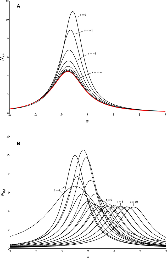
Figure 1. Convergence on the aedt for a one-dimensional landscape. Each curve represents a population distribution, Nx,t, as a function of spatial location, x, for a given value of t, and a given starting time (initial time), s. (A) Backward convergence. The curves from top to bottom represent Nx,t for successively earlier times s, for a fixed value of t, converging on the red curve, which is the aedt, , as s decreases toward –∞ (the distant past). (B) Population distributions, Nx,t, for two different initial distributions, Nx,s (defined by different line types) with fixed s, but changing t. Successive curves to the right represent successive values of t. For large times, the population distributions merge, showing convergence, and hence an aedt.
The Aedt for a Fluid Population
In models, Nt is often assumed to have an initial value at time t = 0, but in aedt theory (Chesson, 2017, 2018), we are interested in how much the current state Nt is affected by past states and past environments. So the initial time must be a variable, s, for which is defined the initial state Ns. The perspective of aedt theory is that initial times and states have no counterpart in nature because ecological systems come into existence by complex idiosyncratic routes, with no specific times and states defining a beginning. This means that serious statements made about them should be independent of initial times and states. An aedt, if it exists, allows such statements.
An aedt can exist in a backward sense, and a forward sense. In the backward sense, is an aedt of Nt if
for every initial fixed state Ns in some suitable set, and all t. The idea is that the present becomes independent of the past. As the initial time retreats into the past, the state at any given time loses any dependence on the initial state, and therefore is simply dependent on the rules for the dynamics of Nt, which reflect the biology of the organisms and the environment they inhabit. The “suitable set” of initial states in the definition might be simply all non-extinct states, or something more restrictive, such as states bounded away from 0 or ∞ as emerges in Box 1, and in non-autonomous dynamics theory (Kloeden and Rasmussen, 2011). Figure 1A illustrates convergence on an aedt in the backward sense. Successively lower curves show Nt for the same fixed value of t = 0, but with s becoming progressively earlier in time. The first curve (s = 0) is Ns, and the red curve on which they all converge as s recedes into the distant past is the aedt, .
In the forward sense, is an aedt of Nt if
for every initial fixed state Ns in some suitable set, and all fixed s. This case can be thought of as meaning that the future becomes independent of the present. Figure 1B shows convergence of two Nt trajectories on each other as time, t, progresses. The initial time, s, is now fixed. The different trajectories, reflecting different starting conditions, are given by different line styles, and successive curves in the positive x direction are successive times. As time progresses, the dashed and solid curve-sequences merge. They have become the aedt. The non-stationarity of the system is seen from the fact that the curves do not approach a limit as t increases. Instead, they simply converge on each other. Note that Figure 1A for backward convergence is from the identical model (to be explained in Box 1) and so also represents a non-stationary system, but as only one value of t is represented, behavior of the model as t changes cannot be inferred from Figure 1A. Figure 1B gives that information.
The importance of the aedt, , is that it defines the trajectory over time that the fluid population will follow if it has been in existence sufficiently long, just as an equilibrium might define the limiting state of the system in a constant environment model. When an aedt exists, it is a critical characteristic defining the long-term pattern of change as determined by the biology of the system and its changing environment. Without an aedt, there may be unlimited possibilities for the pattern of long-term change, and any statement about it would have to be qualified by the assumed initial conditions. It is important to appreciate also that the aedt, , is distinct from the moving equilibrium, , which depends only on the present environmental state, E(t), on the landscape, and has the property Nt+1 = Nt, if Nt = (Chesson, 2017). The moving equilibrium is just the ordinary equilibrium that may exist for the particular state of the environment at time t. Although the moving equilibrium, may, under some circumstances, define were the population is heading at any particular time, as will be discussed further below, only if the environment does not change over time could Nt be expected to converge on .
Population Models
To understand whether an aedt exists, and what its properties are, we need a population model. There can be many different formulations of spatially-dependent population dynamics, depending on the modeling framework and the type of organisms being studied. Terrestrial plants being sedentary, are likely to have spatial structure right down to the smallest scales (Pacala and Silander, 1985; Bolker and Pacala, 1999; Freckleton and Watkinson, 2000). Every point in a landscape is considered as unique. It is somewhat easier conceptually to divide a landscape into patches occupied by multiple individuals within which no spatial structure is recognized. In such models, interactions take place between organisms that occupy a patch at the same time, and patches are connected by movements between them. Such models provide the key example.
Following the framework of Chesson (2000a) and Chesson et al. (2005), a population on a patch x has per capita output λx,t at time t, which corresponds to average individual fitness on the patch. The population density on the patch is Nx,t. So, the total output from the patch is λx,tNx,t, but the population density on the patch is then subject to dispersal, with px,y being the fraction of the population at y that ends up at x. It follows that the population at location x at time t + 1 is
In general, λx,t is a function of the local environment, Ex,t, at location x at time t, and the local population density, Nx,t, at that location,
The environmentally-dependent parameters can be multidimensional. One example, the Beverton-Holt model (Bohner and Warth, 2007; Chesson, 2017), which is a discrete-time version of logistic growth, can be written in the form,
Here, Ex,t is a vector of the two variables, Rx,t and αx,t, where Rx,t is the maximum multiplication rate (traditionally the maximum “finite rate of increase,” which is achieved as the local population approaches 0 density) and αx,t is the intraspecific competition coefficient. In the non-spatial case, this model is known to have an aedt under very mild conditions that simply ensure population viability (Chesson, 2017, 2018). Figure 2 illustrates this model in the spatial case under long-term environmental change.
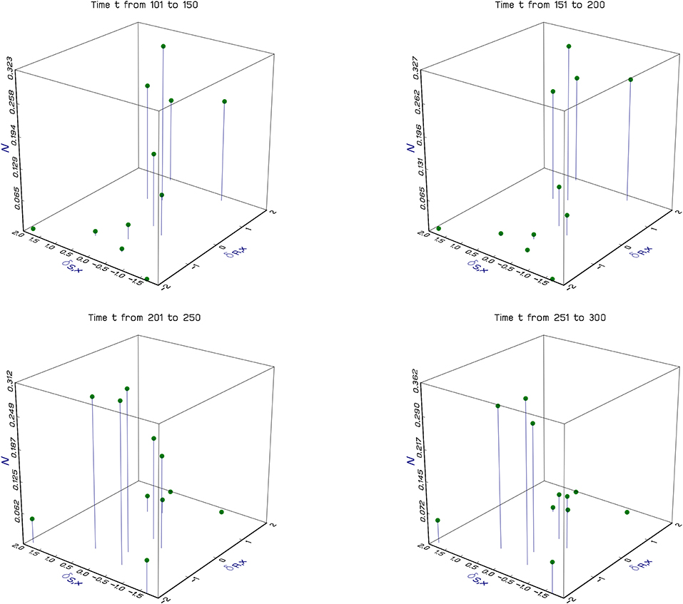
Figure 2. Dynamics of a fluid population on a complex landscape. The figure shows the results of a particular simulation of the Beverton-Holt spatial model (Equations 3–5). Each of the vertical lines in a panel shows the population density of a specific discrete local population. The horizontal plane shows the location in terms of spatial environmental coordinates, δR,x and δS,x (see The experienced environment of the Beverton-Holt). In contrast to Figure 1, where locations are continuous, here locations are discrete, and 100 of them are chosen at random at the beginning of the simulation. Each panel shows no more than 10 locations because only a fraction of the locations have favorable environments for the population in any period of time. Results are averaged over 50 year periods and show the population moving around the landscape as the climate changes. Simulation parameters, δR,x, θR,t, θS,t, and δS,x, are all independent normal with standard deviations respectively 16, 1, 1, and 1, and means 0 except for θR,t which has sine wave variation in the mean with amplitude 2, and period 200 to create non-stationarity; Rmax = Smax = 3; dispersal fraction δ = 0.1.
An alternative to the general discrete-space model (3) is a continuous space form. Then, the sum over y in Equation (3) is replaced by an integral over y, with px,y, replaced by a kernel kx,y, which is the probably density function for movement from location y to location x. In this case, Equation (3) is replaced by
There is no difference in concept between Equations (3) and (6). In both cases, individuals at each location y, measured as Ny,t multiply to λy,tNy,t some of which disperse according to px,y or kx,y to location x. Totaling over y leads to the new population Nx, t+1 at location x. Depending on the description of the environment, this integral over the variable y can be just one dimensional, two dimensional (as would be the case for most terrestrial organisms) or three dimensional (potentially suitable for some marine and atmospheric species). Figure 3, plots a potential dispersal kernel kx,y for a one-dimensional habitat.
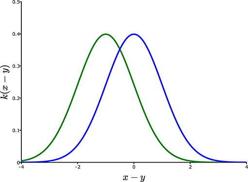
Figure 3. Dispersal shift under linear environmental gradients. The blue curve is a dispersal kernel kx,y for a model showing no directional bias, and no shape change as the location y is changed. Hence, kx,ycan be simply expressed as k(x – y), i.e., simply as a function of the spatial displacement of x from y. Under linear climate change according to the local temperature model θt – δx = θt – δx, global temperature change is equivalent to biased dispersal to the left (increasing temperatures on that landscape) equal to θ/δ, transforming the blue kernel into the green kernel.
Stationarity of the Experienced Environment Under Global Climate Change
Spatial environmental gradients, such as elevational and latitudinal gradients, commonly figure in discussions of climate change because as the climate warms, suitable habitat for an organism is expected to be found at higher elevations or latitudes (Walther et al., 2002). In this section, we show that if the spatial environmental gradient is linear and climate change is linear in time, there can be a general expectation that a population will move up the gradient simply through passive demographic processes, and thereby maintain a stationary experienced environment although the average experienced environment is likely to be suboptimal.
Linear Environmental Gradients
Elevational and latitudinal environmental gradients might be modeled in an additive form where
for some function f, not necessarily linear, global temperature θt is the global temperature at time t, and δx is the adjustment to the global temperature to give the actual temperature T = θt – δx at location x and time t. A simple linear model, which of course is at best an approximation, although commonly used (Berestycki et al., 2009), has θt – δx = θt – δx, where θ and δ are now positive constants. The importance of this case is not realism, but simplicity, which allows a complete solution, and suggests hypotheses for more complex cases that will be considered below (“The experienced environment in complex settings”). In this linear case, for a given time t, location x, and temperature T = θt – δx, we can determine the location that had that temperature at time 0. That location is
This means that organisms that migrate θ/δ spatial units per unit time in the positive x direction would see no change in climate. On the other hand, migrating in the other direction by θ/δ spatial units, per unit time, when the environment is not changing temporally, means the organism would see the temperature increasing by θ units per unit time. These observations show that the presence of climate change in a model can be equivalent to a model with no climate change, but dispersal biased across an environmental gradient. In terms of Figure 3, the blue curve, which gives unbiased dispersal, is replaced by the green curve which is biased to the left. There the kernel, kx,y, takes the form k(x – y), where k is a function of x – y, and thus has the same shape for every location y. The green curve is the kernel k(x – y + θ/δ), which represents a bias in dispersal up the temperature gradient in one unit of time by an amount equivalent to one unit of temporal change in the temperature. This equivalence of biased dispersal and climate change sets the stage for stationarity of the experienced environment.
To see how this equivalence of climate change and environmentally-biased dispersal works out in a model, we introduce the environmental variable ε = –T/δ, which is just temperature converted to equivalent spatial units, and therefore ε = x – (θ/δ)t. At t = 0, ε is simply the spatial location x. So this means that the environment is measured here in terms of environment at specific locations at time 0. Reciprocally, at time t, the location with environment ε is x = ε + (θ/δ)t. If we now define Mε,t to be the population density experiencing environment ε at time t, it follows that
Importantly, the environmentally indexed population density, Mε,t, changes over time in a time-independent way as if there were no climate change, but simply biased dispersal. To see how this works out in the model defined by Equation (6), with the kernel k(x – y), local fitness, λx,t, in the form G(Nx,t, Ex,t) with here Ex,t = f (θt – δx), then
To transform this equation to define the dynamics of Mε,t, we just make the substitutions ε + (θ/δ)(t+1) for x, and ε′ + (θ/δ)t for y because then x has environment ε at time t+1 and y has environment ε′ at time t. Then Equation (10) becomes
In contrast to Equation (10), in Equation (11) the dynamics of the population have no time dependence, because Ex,t = f (θt – δx) has been replaced by , which does not depend on time. However, the dispersal kernel, k(x – y), has been replaced by k(ε − ε′ + θ/δ). Thus, the M process is equivalent to the N process, but with dispersal biased in the direction of increasing temperatures in space, and no temporal change in the environment. The M process tracks the population in environmental coordinates, and relative to these environmental coordinates, the dynamics of population density are not time dependent. Although illustrated here for an integral projection model, the argument is a very general one showing how linear temporal change can be equivalent to biased dispersal on a linear spatial environmental gradient. Note, however, that this outcome does not mean that the experienced environment is stationary. For that the vector Mt of Mε,t values, for all ε, would have to converge on a stationary process with time. For example, Mt might converge on an equilibrium, which is equivalent to the original process Nt having an aedt. We next illustrate this outcome for a simple spatial logistic model.
A simple analytically tractable version of Equation (10) converts it the differential equation model
where g(Nx,t, Ex,t) is the usual continuous-time per capita growth rate rather than the discrete-time multiplication rate G(Nx,t, Ex,t). The dispersal kernel in Equation (12) is very simple: at any instant of time, an individual moves with probability p, or stays put. If it moves, the rate of movement is d spatial units per unit time in the negative x direction. Although greatly oversimplified, this model leads to an explicit solution. Box 1 presents the solution of this model in the case where g(Nx,t, Ex,t) is given by the logistic equation, defining the conditions for aedt to exist as a changing spatial population distribution on a landscape, as illustrated in Figure 1.
Box 1. Non-stationary logistic model with directional dispersal on landscape.
Equation (12) becomes a non-stationary logistic landscape model when g(Nx,t, Ex,t) takes the form
with r being any continuous function, α being a positive continuous function, and θ being the rate at which the physical environmental conditions change with time. The function r defines the maximum growth rate, as a function of the environment, and α defines the intraspecific competition coefficient also as a function of the environment. The environment here is simply measured in spatial units, as x – θt (δ = 1), and this formula means that after one unit of time, the conditions at location x match what they had been at location x – θ. With this formulation, standard solution methods (Miersemann, 2012) give
Note that here the initial distribution on the landscape, Nx,s, is fixed independently of s, i.e., does not vary with s even though the notation is suggestive of it. This system has both forward and backward asymptotic environmentally determined trajectories (aedts), which are identical when the first line in Equation (14) vanishes both as t → ∞, and as s → –∞. The limits are taken separately, i.e., with the other time (either s or t) fixed. These outcomes occur when Nx,sis bounded above zero and the integral of r converges to ∞ as either integration limit becomes infinite. Then, the aedt is given by the equation,
A simple example uses a quadratic form for environmental dependence, with r being a positive constant, and α(x – θt) = α1(x – θt)2, where here on the right α1 is just a constant multiplier of the square.
This special form of the differential equation solves as
which is the basis of the plots in Figure 1. Letting t – s → ∞, leads to the aedt,
The specific logistic model solved in Box 1 has competition coefficient that changes in space according to a quadratic equation
In terms of the usual way of writing logistic competition as g(N) = r(1 – N/K), with intrinsic rate of increase r and carrying capacity, K, we see have K = r/α1(x – θt)2. Thus, the most environmentally favorable place on the landscape at time t is x = θt, where intraspecific competition becomes zero, but this best location shifts with time. Box 1, gives the full solution, and the aedt. Converting the aedt to the ε spatial scale, which represents the population distribution relative to the environment, not relative to fixed spatial locations, the aedt, , is given by the formula
Note that this curve, as a function of ε, does not depend on time. Expressed in climate coordinates, in fact the distribution of the population on the landscape does not change with time when the aedt has been reached, which means that the experienced environment in this case is not merely stationary, but constant, in fact an equilibrium. This curve is plotted in Figure 4 along with the aedt for the case of no climate change. Under climate change, the population retains a unimodal distribution on the landscape. Although the distribution is fixed relative to temperature, the geographic positions corresponding to each temperature (each value of ε) are in fact moving to larger x values, i.e., higher elevations or latitudes. This movement relative to x is shown in Figure 1B.
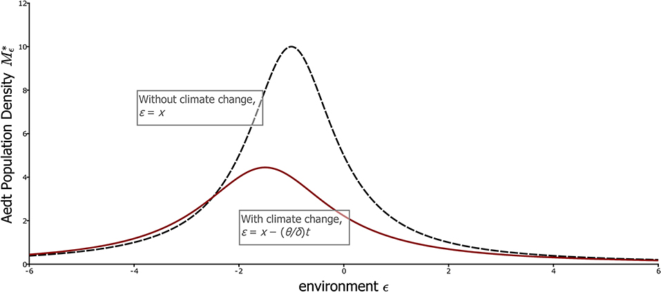
Figure 4. The climate-coordinate aedt for the simple partial differential equation model, with and without climate change. The curves shows the aedt population distribution, , with respect to the climate coordinates ε, with (red) and without (black dashed) climate change. These curves are equilibria when expressed in these coordinates, and thus indicate that the experienced environment is stationary even with climate change. Note that with climate change, population size is lower and peaks further to the left of the most favorable location, ε = 0. Parameters, θ = 0.5 with climate change, 0 without; dp = 1, r = 1, α = 0.1.
Although the climate is stationary in the aedt, climate change naturally still has an effect according to formula (19) as illustrated in Figure 4. The rate of change of global temperature with time is θ, and the mode of the distribution is – (dp + θ)/r in ε coordinates, or (dp + θ)/r directly in temperature units (ε = –T with δ = 1). Thus, we see that the mode is unsurprisingly at higher temperatures under climate change, but the additional temperature at the population mode, θ/r, decreases with the maximum per capita growth rate, r, of a local population. This fact reflects the importance of buildup of the population in favorable locations for it to track climate, an issue that we will return to in more complex settings. The spread of the population relative to climate is also (dp + θ)/r, meaning that faster climate change relative to population growth spreads the population out in climate space. Finally, the total population on the landscape, obtained by integrating Equation (19) from –∞ to ∞, is proportional to r/(dp + θ), and thus decreases with the rapidity of climate change.
This specific example also provides a good illustration of the difference between the aedt and the moving equilibrium. The dashed curve in Figure 4 giving the equilibrium of the population distribution indexed by the environment, Mε,t, when there is no temporal change in the environment, is the same for each fixed level of the global temperature. Thus, it gives the moving equilibrium population distribution too. Like the aedt, the moving equilibrium indexed by the environment is not time-dependent in this case of linear environmental gradients, but is quite different from the aedt, which is given by the red curve of Figure 4.
Although being more complex, and not leading to explicit solutions, Berestycki et al. (2009) show how these general ideas can be realized in models with dispersal represented by diffusion, which is more realistic than the simple flow in one direction specified by the overall rate dp given here. Berestycki et al. (2009) also address the critical question of viability of the population under climate change. In the case where the population might not be able to persist at all in some habitats without dispersal from other areas, climate change that is too rapid may outstrip dispersal, and lead to extinction. Moreover, questions of adaptations to changed conditions naturally become part of the development (Berestycki and Rossi, 2008, 2009; Alfaro et al., 2017).
These models all have the environment changing linearly both in space and time, and have the advantage of leading to clear outcomes. They show that the population can come to equilibrium relative to the environmental gradient, although the gradient itself moves relative to geographical coordinates. But this means that the environment experienced by the population is at equilibrium, which is a very special case of a stationary environment, i.e., one with no temporal change at all. Note that the environment still varies spatially over the range occupied by the population, but does not change with time. One generalization introduces periodic temporal variation, to accommodate seasonality (Berestycki and Rossi, 2009), and then leads to a seasonally varying, but otherwise constant environment experienced by the population. These experienced environments are not the same as the environments experienced without climate change, for as we have seen, they mean that a population may be located suboptimally relative to the environmental gradient, potentially having a smaller population size, and may go extinct. Nevertheless, the temporal stationarity of the experienced environment makes it easy to characterize. Moreover, it provides temporally consistent selection pressures, and means that reasoning about populations relative to stationary environmental conditions retains validity while at the same time adding the extra considerations of the need to follow a population around a landscape, and understand dispersal and population growth processes affecting its movements. The question now is whether such results extend in any suitable sense to more realistic more complex settings, i.e., those not reliant on linear gradients.
The Experienced Environment in Complex Settings
The first task for more complex settings is to define the environment experienced by the population. The physical complexity of landscapes in nature (Alderman and Hinsley, 2007) means that as the climate changes, patterns of physical environmental variation will not merely shift in space as they do in the linear environmental gradients consider above, but will, in general, change in complex ways as a complex topography interacts with regional climate to give local climates. Scale transition theory suggests an approach to understanding experienced environments (Chesson et al., 2005). The theory can be applied to any description of spatial locations, whether as discrete patches, points in an artificial discrete space, or as continuous space, but it is easiest to understand for the discrete-patch definition of a landscape, and thus the population dynamical formulation, Equation (3). The first concept to consider is relative density, νx (ν is Greek nu), which is the local density, Nx, on a patch divided by the regional density:
As suggested by the notation, the regional density, , is equivalent to the spatial average density, at least relative to the total area of the habitat patches (Chesson et al., 2005). In general that means
where px is the fraction of the total habitat area taken up by patch x. In most accounts of scale transition theory, the patches are assumed to be of equal size, meaning that px = 1/k, where k is the total number of habitat patches, but a more general approach is being taken here as more suitable for empirical studies. Indeed, as defined here, the experienced environment can be calculated empirically given the right data.
Having defined the relative density, we can now define the average environment experienced by the population, which needs to be distinguished from the spatial average on the landscape. We can define
which is in fact the average environment over individuals in the population. For example, if there are two sorts of patch of equal area and frequency, but 20% of the population lives in patches with Ex = 1, and 80% in patches with Ex = 2, then , whereas the ordinary spatial average, , equals 0.5 × 1+ 0.5 × 2 = 1.5. The average experienced environment naturally changes as the population moves around on the landscape, and of course as the climate on landscape changes. But these two effects could cancel each other out, as in fact they do in the situation above of linear spatial and temporal environmental change.
Naturally, the experienced variance can be defined, as
Other moments can be defined in the analogous ways, and of course Ex is in general multidimensional as it has been in the all the examples above. Most important, an experienced probably distribution of the environment can be defined by specifying the experienced probability Pν(A) as the probability that an individual randomly chosen from the population experiences environmental states in the set A. The formula for Pν(A) is then
where IA(Ex) is given the value 1 if Ex is in A, and is 0 otherwise. For example, if A is the set “the average annual soil temperature over the year is between 25C and 30C,” then Pν(A) gives the total fraction of the individuals on the landscape experiencing these conditions. All moments, probabilities and other quantities concerning the experienced environment can then be defined in terms of this experienced probability distribution. With a continuous environmental variable, a probability density function would normally define the distribution. Then a probability like (24) would be an area under this probability density function, i.e., the integral over A of this probability density. Figure 4, which gives population density, , as a function of environment, ε, can be used to illustrate experienced environmental distributions as probability densities. Integrating over ε gives the total population size, , and then the experienced environmental probability density function is simply . Integrating fν(ε) over any specific range of ε values gives the fraction of the population experiencing environmental conditions in that range. Thus, the curves in Figure 4 are proportional to the probability density functions for the experienced environment.
In Figure 4, the experienced environments have approached equilibrium, but differ greatly with and without long-term climate change. More generally and realistically, the experienced environmental distribution Pν will fluctuate over time, but we can ask whether these fluctuations are stationary, or approximately so, and how these fluctuations are affected by long-term climate change. The very simplest thing to do is to examine the experienced mean environment (22), which we do next with the Beverton-Holt model. More generally one could ask if the variance (23) of the experienced environment, other moments, and indeed the probabilities (24) show stationary fluctuations over time, and how they differ with and without long-term climate change.
The Experienced Environment of the Beverton-Holt Spatial Model
For the Beverton-Holt model on a landscape (Equations 3–5), we use two orthogonal environmental response variables, Rx,t and Sx,t, defined as functions of the environment at location x and time t. The variable Rx,t is the maximum multiplication rate of the local population at x as represented in the Beverton-Holt formula (5). The variable Sx,t is the local resource supply, with the assumption being that the intraspecific competition coefficient, αx,t, of formula (5) is the ratio Rx,t/Sx,t, in essence, per capita demand over supply.
These environmental response variables are defined as functions of global climate variables θR,t and θS,t, and spatial variables δR,x and δS,x, according to the same kind of additive model (7) as used before
and
Thus, the variables θR,t – δR,x and θS,t – δS,x give the actual value of an environmental variable, such as temperature at location x for time t, and these are then translated into population responses by Equations (25) and (26). Note that these curves are unimodal (proportional to Gaussian curves), and so are maximized for θR,t – δR,x = 0 and θS,t – δS,x = 0, respectively, defining optimal conditions for the local population. In simulations of this model, the underlying environmental variables θR,t, δR,x, θS,t, and δS,x were generated as independent Gaussian variables, with a sinusoidal trend in the mean added to θR,t to make it non-stationary. The idea was not to create and defend a realistic model for some species and landscape in nature, but instead to create a model illustration of the key ideas. Figure 2 illustrates how the population moves around a two-dimensional environmental landscape defined by the axes δR,x and δS,x, i.e., the environments that would occur in space if there were no temporal change.
Dispersal was treated very simply as local retention with widespread dispersal according to the formula,
Thus, in each unit of time, a fraction δ of the population leaves any given site y to settle at random across all sites, including the site y. Though hardly the most realistic form of dispersal, it serves the purpose of simplicity of illustration, both here and later. Figure 5 shows the results of simulating this model giving the experienced mean environments as measured by and which are then compared with spatial average environments and and the environments at the best locations under stationary conditions (Rbest and Sbest). The first 100 years are stationary as a baseline, and after that, sinusoidal temporal variation begins in θR,t showing how the population is pulled around in different directions. The behaviors of Rbest and Sbest reveal the non-stationary conditions that apply at fixed locations, in this case the ones that give the highest values on average, respectively for R and S, during the stationary phase. The non-stationarity of Rbest is clearly evident in the simulations, and naturally it does not remain the best location during the non-stationary phase. Natural Sbest does not show non-stationary as θS,t was simulated as stationary.
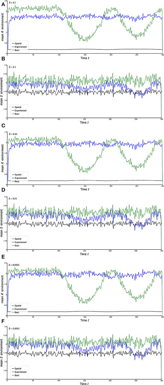
Figure 5. Experienced environments in the Beverton-Holt model. Each of the curves is a plot of a statistic calculated on the landscape for the Beverton-Holt spatial model under climate change. The first 100 years in each case is a stationary initial period after which there is sine wave variation in θR,t with a period of 200 years. In all panels, blue plots are mean experienced environments [and , formula (22) of the text]. The green dashed plots follow the environment of a particular locality. This locality is chosen as the one that gives the highest average value of the variable (R or S) during the stationary phase. Black plots are mean landscape environments unadjusted for the presence of the population ( and ). All parameters as for Figure 2, except for the migration fraction δ, which varies according to the panel. (A,B) δ = 0.1; (C,D) δ = 0.01; (E,F) δ = 0.0001. Each simulation uses the same environmental sequence.
Simplest is the graph of as a function of time for different levels of dispersal. The first message is that is always higher than , and often substantially so. On this landscape remains substantially <1 reflecting the fact that the population has specific habitats within the landscape: it cannot just live anywhere. Second, the clear non-stationarity of Rbest is only to a small extent reflected by . Thus, the experienced mean environment, as judged by , is very close to stationarity. The results for Sx,t give much less pronounced patterns, at least partly due to the lower underlying spatial variance and the absence of non-stationary change in this quantity. However, it is notable that actually shows some non-stationarity despite the fact that there is none in the underlying temporal environmental variable, θS,t. This outcome is likely due to dominance of Rx,t in driving the patterns in λx,t, and hence, as explained below, where the population is to be found. Because Rx,t and Sx,t are statistically independent, dips down to indicating little to no influence of Sx,t on where the population is distributed when Rx,t pulls the population strongly in a particular direction.
Comparing the graphs with different levels of dispersal, no major differences in stationarity of the experienced mean R () are evident, but with high dispersal this experienced mean is low relative to the best location on the landscape under stationarity. This result is understandable from the fact that high dispersal, which is completely passive here, sends a substantial fraction of the population to unfavorable locations. On the other hand, very low dispersal gives values that are quite high both in the stationary and non-stationary phases, but gives a greater degree of non-stationarity in . Intermediate dispersal gives experienced R environments very close to stationary in the non-stationary global change period, while also giving relatively high average values of , suggesting that non-stationarity globally has not greatly affected the population, at least as regards to its experienced R environment.
These results are just simple illustrations of questions and the sorts of answers that might emerge, and are in no way intended as a final analysis of a given situation either in reality or of a model. They raise the question, however, of why we might expect stationarity to emerge even though the environmental gradients are now highly non-linear. Scale transition theory, combined with aedt theory suggests an answer, which we consider next.
Understanding the Dynamics of Experienced Environments Generally
Experienced environments change because the available environments on a landscape, change, organisms disperse across the landscape, and reproduce and survive at rates dependent on their local environments. Here we attempt to disentangle this issue to arrive at an understanding of the general circumstances when experienced environments might show stationary fluctuations over time. We first consider how differences between local environments drive population shifts in the direction of the moving equilibrium (Demographic drivers of distributional change). We then show that under low dispersal, moving equilibria have relatively predictable properties making it possible to identify when the experienced environments predicted from these equilibria might have stationary or approximately stationary temporal dynamics (The moving equilibrium under low dispersal). Finally, we develop the relationship between the moving equilibrium and the aedt, which then provides an indication of the reliability of predictions from the moving equilibrium for the actual experienced environment of the population (Using the moving equilibrium to draw conclusions about the aedt).
Demographic Drivers of Distributional Change
For mean experienced environments, for example as measured by , to show stationary fluctuations over time despite global non-stationarity, population movements on the landscape must somehow cancel out the non-stationary fluctuations. Population movements can be understood in terms of the dynamics or relative density, νx, which, from Equation (3), can be written as
where
Note that ρx,t is relative fitness: the local fitness λx,t compared with population average fitness , which defines landscape-level population change according to scale transition theory (Chesson et al., 2005):
Although, formula (28) is not particularly revealing in this general form, specializing it to widespread dispersal with local retention (formulae (27), as used in the simulations), gives the interpretable form
Here, we see that local relative density increases in proportion to local relative fitness, and thus local density build-up increases with relative fitness, analogous to natural selection of phenotypes, except here it is selection of sites, x, by demography. In this analogy, the dispersing fraction, δ, functions like a mutation rate. If this dispersing faction is high, population build up at favorable sites will be slow and limited, but if the dispersing fraction is low, the fraction retained at a site, 1 – δ, will be high and will promote strong buildup of the population in favorable locations. Note that here dispersal is purely passive, and the gain in relative density is due to high reproduction and survival in favorable sites, not habitat selection or directed dispersal into them.
An indication of how much build-up would occur in favorable locations is given by the equilibrium that Equation (31) implies if in fact the environment did not change over time, but were always at the value applying at time t. This equilibrium is the following very sharply increasing function of relative fitness
where the variables are here indexed by E(x,t) signifying that it the moving equilibrium. At the equilibrium, , which means that = , the value of λx,t at the moving equilibrium, and thus a function of the current environmental conditions. With the Beverton-Holt spatial model, λx,t can be written as
which is an increasing function of both Rx,t and Sx,t, but a decreasing function of νx,t, a relationship that applies also at the equilibrium. It thus follows from Equation (32) that will be maximized at the location where either Rx,t or Sx,t is maximized if the other parameter does not vary in space. These locations x are, respectively, where δR,x most closely matches θR,t or δS,x most closely matches θS,t. In this way, the moving equilibrium is pulled around the landscape by temporal change. In the simulations discussed above, the strong non-stationarity and greater variation in Rx,t did not lead to a appreciably non-stationary . Instead, was notably non-stationary. The explanation seems to be that the population was pulled around the landscape by the maximum in Rx,t leading to approximately experienced stationarity in Rx,t. Strong effects of Rx,t periodically eliminated any sensitivity of the distribution of the population to Sx,t. This effect, along with the statistical independence of Rx,t and Sx,t, explains why would drop to , the ordinary spatial average, as seen in the simulations.
Despite the success of the reasoning above in accounting for the patterns in the simulation, it is important to keep in mind that (32) is the moving equilibrium, and would not ever actually be realized with temporal environmental change. Instead, it merely indicates where Equation (31) would drive the relative densities if in fact the environment remained constant over time at the values applying at time t. Despite this fact, Equation (32) is an important piece in the puzzle. It shows how, at least under widespread dispersal with local retention, the equilibrium relative density can be written directly as function of the environment, and how it changes with time. Equations (28) and (30) can be shown to have a unique globally stable joint equilibrium under the Beverton-Holt model provided all parts of the landscape are accessible over time by dispersal from any other part (Kirkland et al., 2006). Under slow temporal environmental change, this equilibrium will therefore determine how the population is pulled around the landscape. Making the assumption that dispersal is low allows equilibrium, along with stability of the equilibrium, and its implications, to be assessed in other models (Karlin and McGregor, 1972).
The Moving Equilibrium Under Low Dispersal
To solve the low dispersal case, we must step back to consideration of the equilibrium absolute densities, . These can be expressed in terms of equilibrium relative densities, and landscape equilibrium density, , as
Note that in all cases, these equilibria the moving equilibrium. Important questions are whether we would expect these equilibria to exist and be stable beyond the Beverton and Holt model solved by Kirkland et al. (2006). According to Karlin and McGregor (1972), if a stable equilibrium would exist in the absence of dispersal, then the joint connected system would have a stable equilibrium provided the magnitude of dispersal were not too high. In that case also, the equilibrium defined by Equation (34) would exist and would be approximately equal to the equilibrium at location x in the absence of dispersal. In general, however, locations where the population would be extinct in the absence of dispersal would nevertheless have a small positive value for .
Note that the equilibrium in the absence of dispersal is simply a function of the environmental conditions at time t in location x. This means that the corresponding moving equilibrium for the experienced environment is determined simply by the frequency distribution of environmental conditions on the landscape. Thus, if the same sorts of environment conditions continue to exist on the landscape and in the same frequencies, despite climate change, then the moving equilibrium experienced environment would in fact be constant. This is exactly what we see with linear environmental gradients. However, there is nothing to prevent such an outcome with complex non-linear gradients, although the relative positions of the various environment states on the landscape would not remain constant, and a more likely outcome is that the frequency distribution of environmental conditions would only be approximately constant. Moreover, the more general question is stationarity or approximate stationarity of the experienced environment for the moving equilibrium, which would require approximate stationarity of the frequency distribution of environmental states on the landscape.
Using the Moving Equilibrium to Draw Conclusions About the aedt
The results so far allow us to identify at least some general conditions under which the experienced environment of the moving equilibrium would be approximately stationary. These need to be extended to the aedt before they are conclusions about the experienced environment of the population in the long run. Box 2 develops the relationship between the aedt and the moving equilibrium. Although complex, these results show that the aedt can be similar to a moving time average of the moving equilibrium with most weight placed on the most recent times. A complication, however, is that the weights defining this moving average are not constant in general but change with time too. Regardless, these results show that the aedt, , has a fading memory of past environments, with the memory fading more quickly the stronger the stability of the moving equilibrium. In particular, strong stabilizing density dependence means a short memory. One particular consequence is that if the environment shows only slow change temporally, will be close to the moving equilibrium, . Then, if the moving equilibrium gives an approximately stationary experienced environment, so will the aedt. Moreover, the moving time average of stationary process is also a stationary process, which would at first suggest that would give an approximately stationary experienced environment whenever does. However, the weights defining similar to a moving average of change with time too, complicating the picture. On the other hand, there is a reasonable expectation that these weights will change with time in an approximately stationary manner whenever gives a stationary experienced environment. The upshot is that would give an approximately stationary experienced environment whenever does. Further work is needed to confirm this conjecture.
Box 2. The aedt in terms of the moving equilibrium.
According to aedt theory (Chesson, 2017), the aedt (in vector notation as explained above) can be written in terms of the moving equilibrium (in vector notation) according to the formula
where here Ju is the average of the Jacobian matrix (Caswell, 2001) for the landscape model (3) evaluated between and . As explained in Chesson (2017), this equation reduces just to a geometric series in simple cases, and is approximately that if Ju is approximately a constant positive matrix with eigenvalues <1. In general, the formula (35) can be regarded as a generalization of a geometric series, which defines as a generalized moving average of the moving equilibrium . It would thus represent a fading memory of past environmental conditions. However, for Equation (35) to make sense, i.e., for the infinite series to converge, the Jacobian product must converge to 0. In rare instances when this Jacobian is not time-dependent (Chesson, 2017), this sum would converge if the maximum absolute value of its eigenvalues is <1, which is of course the condition for linear stability of the moving equilibrium. In the more usual case of a time-dependent Jacobian, there is no simple necessary and sufficient condition. A simple conservative sufficient condition is that the product of an appropriate matrix norm of the Ju converge to 0 (Bhatia, 1997). One such suitable norm is the singular value norm, which equals the square root of the maximum eigenvalue of (Bhatia, 1997), where the prime means transpose. So rather than consider the maximum eigenvalue of Ju, it is something a little different, viz, the square root of the maximum eigenvalue of a square of the matrix Ju.
Discussion
The non-stationarity of the physical environment over time is a challenge to ecology so accustomed to thinking about nature in terms of equilibria (Cuddington, 2001; Rohde, 2006). A parallel challenge is the complexity of the environment spatially (Hart et al., 2017). Although, most empirical studies have been traditionally conducted on local scales, dissatisfaction with the understanding gained, and recognition that local scales can be dominated by migration and dispersal, have been forcing serious rethinking (Ricklefs, 2008; Hart et al., 2017). The key idea developed here is that the first problem can be resolved by combining it with the second. The key observation is that a population fluid on a landscape can experience approximately a stationary environment as it moves about the landscape even though the environment at any locality is far from stationary.
Here and elsewhere, (Berestycki and Rossi, 2009; Berestycki et al., 2009), exact stationarity of the experienced environment was only shown to occur in the case of a linearly changing spatial environment that combines additively with a linearly changing temporal environment to produce the local environment. Then the environment at a given time and location can be equivalent to the environment at a previous time but a different location, a certain distance away. Dispersal to that location without temporal environmental change thus produces an equivalent outcome. In parlance of dynamical systems theory (Kloeden and Rasmussen, 2011), a non-autonomous system, in which the parameters are time dependent, can be converted into an equivalent autonomous system with no such time dependence of the parameters by the addition of biased dispersal. More realistically, the temporal environmental change might be approximated as a stationary process with a linear trend added (Berestycki and Rossi, 2009). The linear trend could then be equivalent to biased dispersal creating an equivalent system in stationary environment.
The case of a linear trend (Berestycki and Rossi, 2009; Berestycki et al., 2009) is very special, but there is reason to believe that the stationary outcome observed then can be generalized, at least approximately, to more complex temporal change on spatially complex landscapes, as sketched here. There are several components to this. First, favorable locations need to remain present on the landscape, even though they move around, and further the frequencies of environment states at those moving favorable locations need to fluctuate in a stationary manner over time. This means that the equilibria that would occur locally in space, if environment remained fixed, and if there were no dispersal, would indeed define a stationary distribution of experienced environmental states. Second, having some, but not too much dispersal, defines an equilibrium for the landscape, , that inherits the stability properties of the local equilibria. Third, if the temporal trends in the environment are not too great, favorable locations can remain favorable long enough for a population to build up, a process that can work even with passive dispersal. This process was shown above to be analogous to natural selection of phenotypes, but here phenotypes are replaced by spatial locations. Thus, favorable locations are selected rather than favorable phenotypes. Finally, aedt theory shows that if the system has an aedt, the distribution on the landscape may be similar to a moving average over the past to the present of the moving equilibrium, , on the landscape. Under these circumstances it is possible for the aedt to give a stationary experienced environment if the moving equilibrium does. There is much work to be done, however, to confirm and define the limits on these ideas.
These ideas applied complex landscapes were merely illustrated here with limited simulations of a Beverton-Holt model, but they suggest research programs to understand the properties of landscapes, temporal change and biological processes influencing the outcome. Only very simple dispersal was considered in which a fraction of a local population is dispersed at random on the landscape. In this case, the actual spatial configuration of the landscape patches does not matter. Only their environmental states do. Under more localized dispersal, how rapidly the environment changes in space is sure to matter too. Moreover, of the two environmental components considered, only one, R, varied in a non-stationary way. Although the mean experienced environment for R was approximately stationary, that for S was not, even though S was in fact stationary on the landscape. This outcome suggests the capacity for different components of the environment to interact, with some dominating over others and altering their patterns in experienced environments.
Having an approximately stationary experienced environment means that much thinking about populations and communities on local scales for stationary environments is potentially transferable to fluid populations and communities with non-stationary environmental variation. However, it also means paying more attention to the role of dispersal processes, the complexity of landscapes, the nature of temporal environmental change, and their interactions. Not only do these issues affect whether experienced environments will be roughly stationary, but they also affect what those experienced environments are like, for example, simply their overall quality.
Missing from the development here was any significant consideration of the role of adaptation. The population parameters as a function of the environment were here assumed fixed, but most serious discussions of climate change naturally consider adaptation (Davis and Shaw, 2001; Davis et al., 2005; Norberg et al., 2012; Urban et al., 2016). Significantly, critical work on linear environmental change (Alfaro et al., 2017) already points the way forward. Natural selection might also select for dispersal ability under non-stationary change (Weiss-Lehman et al., 2017) further modifying experienced environmental distributions.
Although the focus here has been on single species, it is clear that some aspects extend just as well to communities. Transforming linear temporal change to biased dispersal without temporal change applies equally to communities as to single populations, provided there is just a single environmental variable. However, realistic variation on complex landscapes must inevitably magnify the effects of interactions between environmental variables evident here even in a single-species case. Differential responses to the environment (Spear et al., 1994; Tingley et al., 2012), dispersal abilities, and population turnover rates (Davis, 1986) may well-enhance the differences between species, greatly affecting the outcomes of their interactions when considered in the long-run (Bolker and Pacala, 1999). There is great potential for rich new understanding of communities focused on these various implications of long-term environmental change.
Science is at the beginning of enormous challenges of ecology under changing environments (Urban et al., 2016). Although the focus here has been simply on climate change, land use change has perhaps been the most pronounced effect so far of the Anthropocene (Tingley et al., 2013). Habitat destruction and habitat fragmentation alter the basic landscape structure and dispersal processes that are central to the effects of climate change as discussed here. For some organisms, landscape change might be regarded as simply another form of environmental change fitting within this framework. Although the ability to transform a new situation to old one, which has been explored here, might be applicable in some cases, at the present time there is no substitute for multiple and diverse approaches. Yet, as is shown here and elsewhere, answers to new problems may well-reside in old problems examined in a new light (Bolker and Pacala, 1999).
Author Contributions
PC conceived of the project, developed the theory, and wrote the manuscript. PY wrote the code for the simulations.
Funding
This work was supported by NSF grant DEB-1119784.
Conflict of Interest
The authors declare that the research was conducted in the absence of any commercial or financial relationships that could be construed as a potential conflict of interest.
Acknowledgments
We are grateful for discussions of this work during its development with Galen Holt, Brett Melbourne, and Yi-Jie Wu.
References
Abrams, P. (1984). Variability in resource consumption rates and the coexistence of competing species. Theor. Popul. Biol. 25, 106–124. doi: 10.1016/0040-5809(84)90008-X
Alderman, J., and Hinsley, S. A. (2007). Modelling the third dimension: incorporating topography into the movement rules of an individual-based spatially explicit population model. Ecol. Compl. 4, 169–181. doi: 10.1016/j.ecocom.2007.06.009
Alfaro, M., Berestycki, H., and Raoul, G. (2017). The effect of climate shift on a species submitted to dispersion, evolution, growth and nonlocal competition. SIAM J. Math. Anal. 49, 562–596. doi: 10.1137/16M1075934
Andrewartha, H. G., and Birch, L. C. (1954). The Distribution and Abundance of Animals. Chicago, IL: University of Chicago Press.
Andrewartha, H. G., and Birch, L. C. (1984). The Ecological Web: More on the Distribution and Abundance of Animals. Chicago, IL: Chicago University Press.
Berestycki, H., Diekmann, O., Nagelkerke, C. J., and Zegeling, P. A. (2009). Can a species keep pace with a shifting climate? Bull. Math. Biol. 71, 399–429. doi: 10.1007/s11538-008-9367-5
Berestycki, H., and Rossi, L. (2008). Reaction-diffusion equations for population dynamics with forced speed I - The case of the whole space. Discrete Cont. Dyn. Syst. 21, 41–67. doi: 10.3934/dcds.2008.21.41
Berestycki, H., and Rossi, L. (2009). Reaction-diffusion equations for population dynamics with forced speed II - cylindrical-type domains. Discrete Cont. Dyn. Syst. 25, 19–61. doi: 10.3934/dcds.2009.25.19
Bohner, M., and Warth, H. (2007). The Beverton–Holt dynamic equation. Appl. Anal. 86, 1007–1015. doi: 10.1080/00036810701474140
Bolker, B. M., and Pacala, S. W. (1999). Spatial moment equations for plant competition: understanding spatial strategies and the advantages of short dispersal. Am. Nat. 153, 575–602. doi: 10.1086/303199
Bowler, D. E., Heldbjerg, H., Fox, A. D., O'Hara, R. B., and Bohning-Gaese, K. (2018). Disentangling the effects of multiple environmental drivers on population changes within communities. J. Anim. Ecol. 87, 1034–1045. doi: 10.1111/1365-2656.12829
Caswell, H. (2001). Matrix Population Models: Construction: Analysis and Interpretation. Sunderland, MA: Sinauer Associates.
Chesson, P. (1991). A need for niches? Trends Ecol. Evol. 6, 26–28. doi: 10.1016/0169-5347(91)90144-M
Chesson, P. (1994). Multispecies competition in variable environments. Theor. Popul. Biol. 45, 227–276. doi: 10.1006/tpbi.1994.1013
Chesson, P. (2000a). General theory of competitive coexistence in spatially-varying environments. Theor. Popul. Biol. 58, 211–237. doi: 10.1006/tpbi.2000.1486
Chesson, P. (2000b). Mechanisms of maintenance of species diversity. Annu. Rev. Ecol. Syst. 31, 343–366. doi: 10.1146/annurev.ecolsys.31.1.343
Chesson, P. (2017). AEDT: a new concept for ecological dynamics in the ever-changing world. PLoS Biol. 15:e2002634. doi: 10.1371/journal.pbio.2002634
Chesson, P. (2018). Contributions to nonstationary community theory. J. Biol. Dyn. 13(suppl. 1):123–150. doi: 10.1080/17513758.2018.1526977
Chesson, P., Donahue, M. J., Melbourne, B. A., and Sears, A. L. W. (2005). “Scale transition theory for understanding mechanisms in metacommunities,” in Metacommunities: Spatial Dynamics and Eclogical Communities, eds M. Holyoak, M. A. Leibold, and R. D. Holt (Chicago, IL: The University of Chicago Press, 279–306.
Cuddington, K. (2001). The “Balance of Nature” metaphor and equilibrium in population ecology. Biol. Phil. 16, 463–479. doi: 10.1023/A:1011910014900
Davis, M. B. (1986). “Climatic instability, time-lags and community disequilibrium,” in Community Ecology, eds J. Diamond and T. Case (Cambridge: Harper and Row, 269–284.
Davis, M. B. (1994). Ecology and paleoecology begin to merge. Trends Ecol. Evol. 9, 357–358. doi: 10.1016/0169-5347(94)90049-3
Davis, M. B., and Shaw, R. G. (2001). Range shifts and adaptive responses to quaternary climate change. Science 292, 673–679. doi: 10.1126/science.292.5517.673
Davis, M. B., Shaw, R. G., and Etterson, J. R. (2005). Evolutionary responses to changing climate. Ecology 86, 1704–1714. doi: 10.1890/03-0788
Freckleton, R. P., and Watkinson, A. R. (2000). On detecting and measuring competition in spatially structured plant communities. Ecol. Lett. 4, 432–432. doi: 10.1046/j.1461-0248.2000.00167.x
Harsch, M. A., Zhou, Y., HilleRisLambers, J., and Kot, M. (2014). Keeping pace with climate change: stage-structured moving-habitat models. Am. Nat. 184, 25–37. doi: 10.1086/676590
Hart, S. P., Usinowicz, J., and Levine, J. M. (2017). The spatial scales of species coexistence. Nat. Ecol. Evol. 1, 1066–1073. doi: 10.1038/s41559-017-0230-7
Huxman, T. E., Kimball, S., Angert, A. L., Gremer, J. R., Barron-Gafford, G. A., and Venable, D. L. (2013). Understanding past, contemporary, and future dynamics of plants, populations, and communities using sonoran desert winter annuals. Am. J. Bot. 100, 1369–1380. doi: 10.3732/ajb.1200463
Ignace, D. D., Huntly, N., and Chesson, P. (2018). The role of climate in the dynamics of annual plants in a Chihuahuan Desert ecosystem. Evol. Ecol. Res. 19, 279–297. Available online at: http://www.evolutionary-ecology.com/issues/v19/n03/ffar3143.pdf
Jackson, S. T. (2012). “Conservation and resource management in a changing world: extending historical range of variation beyond the baseline,” in Historical Environmental Variation in Conservation and Natural Resource Management (Chichester: John Wiley and Sons, Ltd.), 92–109. doi: 10.1002/9781118329726.ch7
Jackson, S. T., and Blois, J. L. (2015). Community ecology in a changing environment: perspectives from the quaternary. Proc. Natl. Acad. Sci. U.S.A. 112, 4915–4921. doi: 10.1073/pnas.1403664111
Jackson, S. T., and Overpeck, J. T. (2000). Responses of plant populations and communities to environmental changes of the late Quaternary. Paleobiology 26, 194–220. doi: 10.1017/S0094837300026932
Jones, P. D., Briffa, K. R., Barnett, T. P., and Tett, S. F. B. (1998). High-resolution palaeoclimatic records for the last millennium: interpretation, integration and comparison with General Circulation Model control-run temperatures. Holocene 8, 455–471. doi: 10.1191/095968398667194956
Karlin, S., and McGregor, J. (1972). Polymorphisms for genetic and ecological systems with weak coupling. Theor. Popul. Biol. 3, 210–238. doi: 10.1016/0040-5809(72)90027-5
Kirkland, S., Li, C. K., and Schreiber, S. J. (2006). On the evolution of dispersal in patchy landscapes. SIAM J. Appl. Math. 66, 1366–1382. doi: 10.1137/050628933
Kloeden, P. E., and Rasmussen, M. (2011). Nonautonomous Dynamical Systems. Providence, RI: American Mathematical Society. doi: 10.1090/surv/176
Levins, R. (1979). Coexistence in a variable environment. Am. Nat. 114, 765–783. doi: 10.1086/283527
MacArthur, R. (1970). Species packing and competitive equilibrium for many species. Theor. Popul. Biol. 1, 1–11. doi: 10.1016/0040-5809(70)90039-0
Marsicek, J., Shuman, B. N., Bartlein, P. J., Shafer, S. L., and Brewer, S. (2018). Reconciling divergent trends and millennial variations in Holocene temperatures. Nature 554, 92–96. doi: 10.1038/nature25464
May, R. M. (1974). Stability and Complexity in Model Ecosystems, 2nd Edn. Princeton, NJ: Princeton University Press.
McDowell, P. F., Webb, T. III., and Bartlein, P. J. (1995). “Long-term environmental change,” in Ecological Time Series, eds T. M. Powell and J. H. Steele (New York, NY: Chapman and Hall), 327–370. doi: 10.1007/978-1-4615-1769-6_16
Miersemann, E. (2012). Partial Differential Equations: Lecture Notes. Leipzig: University of Leipzig.
Montoro Girona, M., Navarro, L., and Morin, H. (2018). A secret hidden in the sediments: lepidoptera scales. Front. Ecol. Evol. 6:2. doi: 10.3389/fevo.2018.00002
Murdoch, W. W. (1994). Population regulation in theory and practice. Ecology 75, 271–287. doi: 10.2307/1939533
Murdoch, W. W., Briggs, C. J., and Nisbet, R. M. (2003). Consumer-Resource Dynamics. Princeton, NJ: Princeton University Press.
Navarro, L., Harvey, A. -É., Ali, A., Bergeron, Y., and Morin, H. (2018a). A Holocene landscape dynamic multiproxy reconstruction: how do interactions between fire and insect outbreaks shape an ecosystem over long time scales? PLoS ONE 13:e0204316. doi: 10.1371/journal.pone.0204316
Navarro, L., Morin, H., Bergeron, Y., and Girona, M.M. (2018b). Changes in spatiotemporal patterns of 20th century spruce budworm outbreaks in eastern canadian boreal forests. Front. Plant Sci. 9:1905. doi: 10.3389/fpls.2018.01905
Norberg, J., Urban, M. C., Vellend, M., Klausmeier, C. A., and Loeuille, N. (2012). Eco-evolutionary responses of biodiversity to climate change. Nat. Clim. Change 2, 747–751. doi: 10.1038/nclimate1588
Pacala, S. W., and Silander, J. A. Jr. (1985). Neighborhood models of plant population dynamics. I. Single-species models of annuals. Am. Nat. 125, 385–411. doi: 10.1086/284349
Ricklefs, R. E. (2008). Disintegration of the ecological community. Am. Nat. 172, 741–750. doi: 10.1086/593002
Ripa, J., and Ives, A. R. (2003). Food web dynamics in correlated and autocorrelated environments. Theor. Popul. Biol. 64, 369–384. doi: 10.1016/S0040-5809(03)00089-3
Rohde, K. (2006). Nonequilibrium Ecology. New York, NY: Cambridge University Press. doi: 10.1017/CBO9780511542152
Scudo, F. M. (1984). The “Golden Age” of theoretical ecology; a conceptual appraisal. Rev. Eur. Sci. Soc. 22, 11–64.
Spear, R. W., Davis, M. B., and Shane, L. C. K. (1994). Late quaternary history of low-elevation and mid-elevation vegetation in the white mountains of New-Hampshire. Ecol. Monogr. 64, 85–109. doi: 10.2307/2937056
Strong, D. R. (1986). “Density vagueness: abiding the variance in the demography of real populations,” in Community Ecology, eds J. Diamond and T. E. Case (New York, NY: Harper and Row Publishing), 257–268.
Tilman, D. (1982). Resource Competition and Community Structure. Princeton, NJ: Princeton University Press.
Tingley, M., Estes, L., and Wilcove, D. (2013). Ecosystems: climate change must not blow conservation off course. Nature 500, 271–272. doi: 10.1038/500271a
Tingley, M. W., Koo, M. S., Moritz, C., Rush, A. C., and Beissinger, S. R. (2012). The push and pull of climate change causes heterogeneous shifts in avian elevational ranges. Global Change Biol. 18, 3279–3290. doi: 10.1111/j.1365-2486.2012.02784.x
Urban, M. C., Bocedi, G., Hendry, A. P., Mihoub, J.-B., Pe'er, G., Singer, A., et al. (2016). Improving the forecast for biodiversity under climate change. Science 353:aad8466. doi: 10.1126/science.aad8466
Walther, G.-R., Post, E., Convey, P., Menzel, A., Parmesan, C., Beebee, T. J., et al. (2002). Ecological responses to recent climate change. Nature 416:389. doi: 10.1038/416389a
Keywords: non-stationary environment, aedt, landscape, scale transition theory, experienced environment, climate change
Citation: Chesson P and Yang PJ (2019) Populations as Fluid on a Landscape Under Global Environmental Change. Front. Ecol. Evol. 7:363. doi: 10.3389/fevo.2019.00363
Received: 03 December 2018; Accepted: 12 September 2019;
Published: 27 September 2019.
Edited by:
Andrew J. Rominger, Santa Fe Institute, United StatesReviewed by:
Annette Ostling, University of Michigan, United StatesMiguel Montoro Girona, Swedish University of Agricultural Sciences, Sweden
Jacopo Grilli, Santa Fe Institute, United States
Copyright © 2019 Chesson and Yang. This is an open-access article distributed under the terms of the Creative Commons Attribution License (CC BY). The use, distribution or reproduction in other forums is permitted, provided the original author(s) and the copyright owner(s) are credited and that the original publication in this journal is cited, in accordance with accepted academic practice. No use, distribution or reproduction is permitted which does not comply with these terms.
*Correspondence: Peter Chesson, cGNoZXNzb25AZW1haWwuYXJpem9uYS5lZHU=