
94% of researchers rate our articles as excellent or good
Learn more about the work of our research integrity team to safeguard the quality of each article we publish.
Find out more
ORIGINAL RESEARCH article
Front. Environ. Sci. , 16 October 2020
Sec. Toxicology, Pollution and the Environment
Volume 8 - 2020 | https://doi.org/10.3389/fenvs.2020.525469
This article is part of the Research Topic The Urban Critical Zone View all 4 articles
The Milano Metropolitan Area [named FUA (functional urban area)] has a history of heavy industrialization causing a large portion of area being affected by significant diffuse contaminations of soil and groundwater. Among the various contaminants, chlorinated solvents (e.g., tetrachloroethylene and trichloroethylene) are the most used in industrial processes and represent the major cause of groundwater pollution within the FUA. The background diffuse contamination generated by these pollutants is so persistent and widely spread that makes it extremely challenging to identify the sources responsible for their release. Such background contamination originates from the overlapping of both known sources (point sources), associated to specific high release of contamination, and unknown small sources (multiple point sources), clustered within a large area, whose release is low but persistent. The aim of this article is to present the methodology, developed within the framework of the AMIIGA Project (Interreg Central Europe Grant N° CE32), which combines multivariate statistical analysis and groundwater numerical modeling in order to separate the point sources contribution from the background diffuse contamination, and supporting public authorities in the management of groundwater remediation. A methodological workflow is proposed guiding local and regional institutions to use the methodology (i.e., exploratory analysis of big dataset, simulation of groundwater flow and transport, multivariate and geostatistical analysis) to assess diffuse pollution background levels in large urbanized areas.
Groundwater contamination by chlorinated solvents is a critical issue (Alamdar et al., 2019) in functional urban areas (FUAs, OECD, 2012). According to Alberti et al. (2018) such contamination is typically associated to point sources (PSs) corresponding to hotspots releasing plumes of high concentrations. However, because of the intense industrial and urban development during the last postindustrial years, in FUA there are a number of unknown small sources releasing a low contaminant mass. These multiple PSs (MPSs) may originate from sewage system leakages, small garages, or single spill of paints by single citizens, and MPSs are often responsible in urban areas of a diffuse background contamination. In Italy, the Italian legislative decree (IT-Decree 3/04/2006.n. 152, 2006, which enforce the Water Framework Directive) defines the anthropogenic diffuse pollution as the “chemical, physical, and biological alteration of environmental matrixes and contaminations determined by diffuse sources and not linked to a PS,” and it designates regional authorities to recognize and to enact actions when diffuse contamination is identified. Because of this legislative demand, there is the need of scientific-based tools as support for recognizing areas affected by anthropogenic diffuse pollution and identifying proper diffuse pollution background levels (DPBLs) (i.e., background diffuse pollution level not attributable to specific PSs).
In urban areas, highly contaminated plumes coexist with diffuse background contamination. Within the Milano FUA, a background diffuse contamination is present with concentration levels that are higher than the environmental quality standard (EQS) for PCE defined by the IT-Decree 3/04/2006.n. 152, 2006). In the same area, highly polluted plumes pose challenges in terms of the assessment of contaminant migration pathways, identification of the source (Alderuccio et al., 2019; Colombo et al., 2019; Ostoich et al., 2019; Stefania et al., 2019), and remediation activities. In areas where a diffuse contamination background is present, site owners and stakeholders, not directly responsible for the contamination, often have to cope with unsustainable remediation and groundwater protection costs.
Although clearly stated that measures to recover diffuse pollution of groundwater contribute to the achievement of quality goals for both groundwater and surface water bodies defined under the WFD, no specific mention about the need to manage identify groundwater diffuse pollution background levels is given in these directives. In 2006, Italian Legislative Decree 152/06 enforcing the EU-WFD (EU-Directive 2006/118/CE, 2006; Balderacchi et al., 2014) defined water quality objectives to be achieved by 2015 (with the possibility to extend the time of achievement). The aim was to regulate procedures at the scale of groundwater bodies and to leave the responsibility to each member state for groundwater management (as reflected by the IT-Decree 3/04/2006.n. 152, 2006). However, it was early clear that member states had local critical situations hampering the respect of the objectives due to the occurrence of anthropogenic diffuse contaminated areas, particularly in urban settings (Busico et al., 2018; Alamdar et al., 2019; La Vigna et al., 2019; Pereira, 2019). Such “diffuse-like” contamination originated from former unknown PSs (i.e., MPSs) is totally neglected in existing European legislation, and only at regional scale some legislations exist addressing this issue (Regione Lombardia, 2017). Dealing with groundwater contamination at the urban scale is in fact in the loophole between EU regulation (e.g., large diffuse nitrate contamination) and national legislations (PSs). The anthropogenic diffuse contamination in urban aquifers cannot be managed with the usual remediation strategies used for PSs, for two main reasons: (1) the difficulty to identify specific sources and (2) the broad extension of the contaminated areas. Both aspects call for alternative approaches, because the application of standard characterization and remediation strategies are not economically sustainable.
Several well-established methodological approaches exist for the identification of natural background level (NBL) of groundwater contaminants (Rotiroti and Fumagalli, 2013; Rotiroti et al., 2015; Ducci et al., 2016; Parrone et al., 2019; Serianz et al., 2020). However, consolidated methods are still lacking for the identification of DPBLs. In this study, the multivariate statistical approach described by Azzellino et al. (2019) has been combined with numerical modeling and geostatistics to support definition of DPBLs.
The study concerns the northwestern (NW) sector of the Milano FUA, where a widespread groundwater contamination is present mainly due to tetrachloroethylene (PCE). In this area, single plumes with higher contaminant concentration deriving from a known source of contamination coexist with a broad background diffuse contamination, characterized by lower concentration levels (but still higher than legal threshold limits defined in the IT-Decree 3/04/2006.n. 152, 2006). In such complex settings, main challenges are either the capability to locate sources (Alberti et al., 2016a; Bortoni et al., 2019) and to track the plumes (Stefania et al., 2018; Colombo et al., 2019) or to define the DPBLs representative for the broad area to which the plumes overlap (Azzellino et al., 2019). Improving the capability of tracking plumes and the apportionment of contaminant sources will make remediation strategies more effective, allowing to identify the polluter, which should be charged with the liability costs for remediation (Alderuccio et al., 2019). Concerning PCE, a range of remediation technologies can be used, ranging from adsorption on granular activated carbon (Erto et al., 2009) or on clay minerals (Cloutier et al., 2008) to biodegradation (Wang et al., 2020) and degradation in catalyzed systems (Watts and Teel, 2019), with costs dramatically different whether the source of pollution is diffuse or localized. On the other hand, the definition of DBPLs would allow to quickly identify situations where the treatment costs would be extremely high and the remediation largely ineffective, preventing to charge expensive and ineffective remediation measures to site owners not responsible for the groundwater contamination. We believe that this study will be useful to propose a decisional framework of methods useful to estimate DPBLs for groundwater contaminated by chlorinated solvents and any other kind of pollutants.
The study area is located in the Lombardy Region, encompassed between the main rivers Ticino and Adda, located to the west and to the east of Milano, and it includes the NW sector of Milano city and 12 municipalities belonging to the FUA. The total area is 157 km2 and lies at the center of one of the most populated and industrialized areas in Europe (Figure 1). The area is historically affected by the presence of many chlorinated hydrocarbons plumes originating from the northern outer border of the Milano municipality where many suspected contaminated sites (as brownfields and active industrial sites) are present, which had been or are still active during most of 20th century.
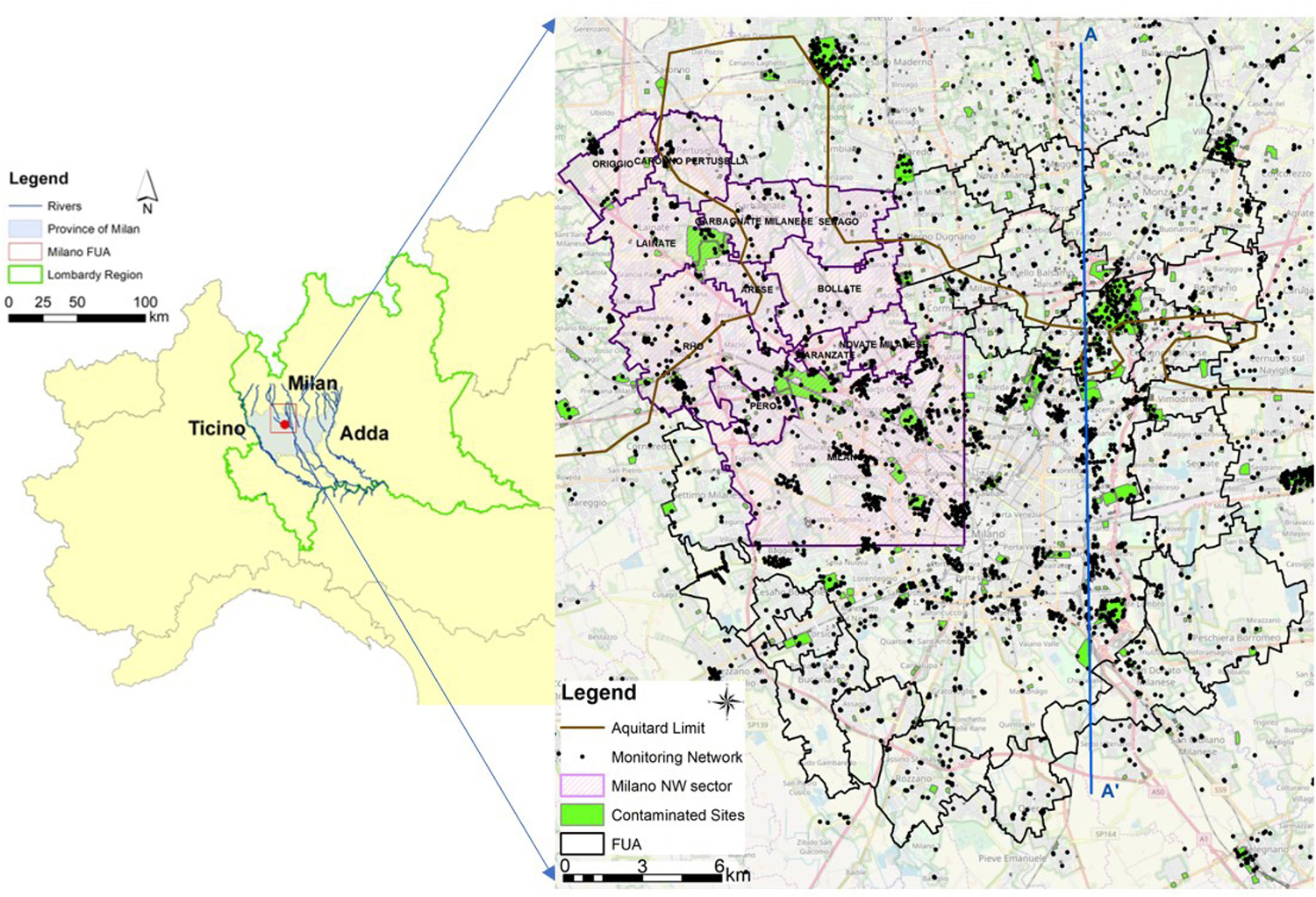
Figure 1. Study area and distribution of available monitoring network and contaminated sites. The pilot area in the right is colored by pink (12 municipalities: Milano, Pero, Rho, Baranzate, Novate M.se, Bollate, Arese, Senago, Garbagnate M.se, Lainate, Caronno Pertusella and Origgio). The Milano Province on the left is dashed with gray color.
Local hydrology is dominated by the Seveso and Olona rivers and the Villoresi irrigation channel (Figure 2). The mean annual temperature and precipitation are, respectively, 15°C and 1,200 mm. The main direction of the groundwater flow is from north–northwest to southeast with an average groundwater gradient of 0.2%. Four main aquifer Group (named from A to D) are recognized in the Lombardy Plain, but only three have been investigated through drillings in the Milano area. The aquifers are hosted by a sequence of plio-pleistocenic alluvial sediments that filled the Neogene Po plain foredeep reaching a maximum thickness of approximately 500 m (Bini, 1997; Carcano and Piccin, 2002).
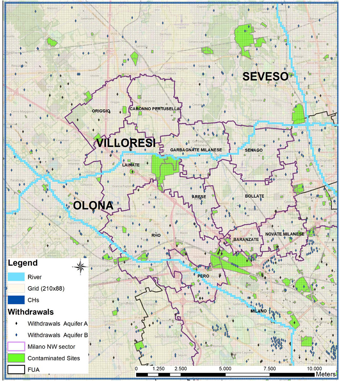
Figure 2. Model domain, internal conditions (rivers in light blue), and wells (divided in the two aquifers based on the screens position). For more details about the model implementation, see Supplementary Figure S1 (Colombo et al., 2019).
The main aquifers affected by the contamination (A and B) have an alluvial and glaciofluvial origin and have the highest transmissivity values. The shallow Aquifer A has an average thickness of 30 m and is composed of sandy-gravel with hydraulic conductivity ranging between 1 × 10⁻⁵ and 4 × 10⁻³ m/s. Underneath, the semiconfined Aquifer B, about 60 m thick, is characterized by a hydraulic conductivity varying between 1 × 10⁻⁵ and 1.4 × 10⁻³ m/s. This unit is mainly composed of sand interrupted by clay lenses that subdivide it in several small aquifers (i.e., multilayered aquifer). The two aquifers are hydraulically unseparated in the northern part of the study area (Figure 3); i.e., it exists only an unconfined, unseparated/undifferentiated aquifer constituted by both Aquifers A and B, shown in Figure 1 above the aquitard limit (brown line). The absence of hydraulic separation between the two aquifers is also shown in Figure 3, where the clay lenses in black disappear proceeding toward Monza. On the other hand, in the Milano area, Aquifers A and B are hydraulically separated at a depth of about 40 m from the ground level by a clay layer (black lenses in Figure 3, with thickness varying between 5 and 10 m) with a very low hydraulic conductivity (around 1 × 10⁻⁹ m/s). More details about the conceptual model can be found in previous works (Cavallin et al., 1983; Alberti and Francani, 2001; Perego et al., 2014; ARPA Lombardia, 2015; Alberti et al., 2016b). A proper definition of the aquifer geometry and hydrogeological properties is a key step to clearly define how monitoring well screens are distributed in the overlapping aquifers, to properly define the monitoring networks and to build a mathematical model useful to reconstruct the groundwater flow and contaminant transport.
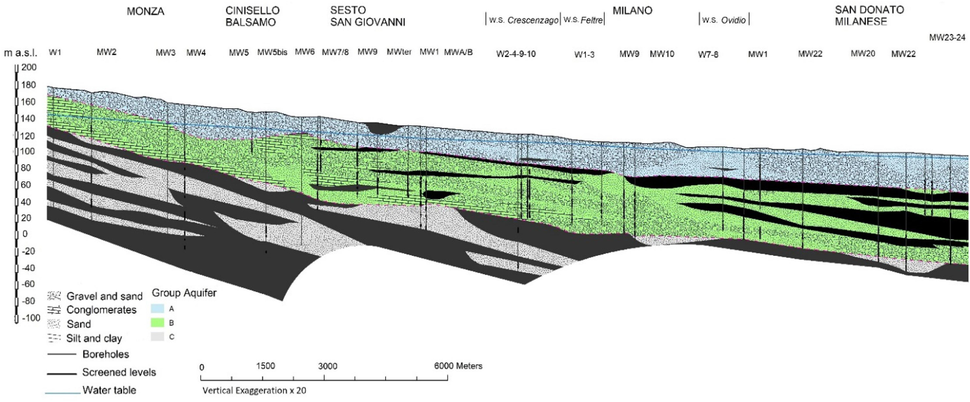
Figure 3. North-South cross section AA’ corresponding to the blue line in Figure 1. Aquifers A and B are in light blue and green.
The methodology developed during the Interreg Project (AMIIGA-CE32) is summarized in Figure 4. The proposed approach has a key role to assess DPBLs in urban areas, and it is shown as a step-by-step decisional framework where the main steps are summarized in the flowchart.
The methodology developed in this article, from the preliminary data exploration by means of multivariate statistical analysis through the coupling with a groundwater fate and transport model, consists of five main steps:
(1) Data collection and preparation: gathering of data available in Milano FUA (concentration values, monitoring network characteristics, documentary research on contaminates sites) and setup of the database structure (detection of outliers, errors, and missing values).
(2) Exploratory data analysis: cluster analysis (CA) applied to a univariate set of concentration data (PCE) in order to separate the PS hotspots from the background diffuse pollution due to MPSs. The identified hotspots (if associated to some documental information) are used as input contamination sources for the numerical model.
(3) Numerical modeling (MODFLOW2005+MT3DMS): simulation based on the identified hotspots of the main contamination plumes in the FUA. The model results are useful to separate the dataset in 2 main components: the first one linked to specific PSs and a second one, larger and clustered in overall area, not linked to any hotspot that can be associated to a diffuse contamination (Colombo et al., 2019).
(4) Multivariate analysis: principal component and factor analysis (PCA/FA) with CA to identify the different water quality profiles of diffuse contamination in the FUA (Azzellino et al., 2019).
(5) Spatial analysis: the diffuse contamination pattern is analyzed by means of spatial interpolation tools.
These steps will be further explained and described in the following paragraphs and will be applied to the NW Milano part of the FUA case study, in order to demonstrate how the DPBLs may be defined.
For the assessment of groundwater quality, 10 independent geochemical datasets, provided by private and regional agencies (e.g., Water Managers and the Environmental Protection Agency) were merged into a single database. It contains structural information about 3,500 wells/piezometers (name of monitoring point, address and municipality, site owner, geographical coordinates, depth of monitoring point, and screen information) and 12 hydrochemical groundwater data (as shown in Table 1, the variables are in the first column) covering the period 2003–2017. The descriptive statistics in Table 1 provided details regarding mean, median, standard deviation, maximum, minimum, and main quartiles. Once the data were collected, the final data needed to be checked, validated, and prepared prior to proceeding with the following data analysis. The steps involved data editing and coding (e.g., check for errors or omissions) and data cleaning (e.g., error detection and treatment of missing data). One of the most important steps was to detect errors and omissions and, in general, to check whether the data complied with the required quality standards (accurate, consistent with goal, uniformly entered, complete, and with a good codification and tabulation). The final dataset was validated in collaboration with the Environmental Protection Agency (i.e., comparing data entry with sampling certificates). At this stage, a univariate CA was applied to PCE concentrations (Afifi et al., 2003; Everitt et al., 2011; Yu et al., 2014) to identify data errors, outliers, and measurements strictly linked to hotspots (i.e., PSs).
As described by Azzellino et al. (2019) a k-means clustering algorithm was applied, which, starting from k seeds or initial centers, allowed to isolate k clusters of similar characteristics. The k-means procedure was applied to all available data of PCE groundwater measurements containing both background values and several outliers. Based on different trials, k was set to 15, and the analysis was run twice, using the final cluster centroids, obtained from the first analysis, as initial seeds for the second. Some of the identified clusters were clearly contamination hotspots and were considered later as PSs in the modeling phase. A multivariate k-means CA was also applied later to identify patterns (i.e., clusters) of background diffuse pollution in the Milano FUA.
A three-dimensional (3D) numerical flow and transport model was implemented using MODFLOW2005 (Harbaugh, 2005) and MT3DMS (Zheng, 2010) through the graphical interface Groundwater Vistas 6. A period of 63 years was used as total transport simulation time (starting from 1955 to 2017) in order to simulate historical plumes linked to the oldest sources. This allowed reaching a quasi–steady-state for PCE level simulation downstream of the main industrial plants selected as PSs. The advective term of the transport was solved using the total variation diminishing scheme because it is more accurate in solving advection-dominated problems and minimizing numerical dispersion (Zheng and Wang, 1999; Zheng, 2010). Plume simulation showed the extent of the PS contamination in the area. More details about flow (e.g., grid, boundary and internal conditions, hydraulic conductivity) and transport model (e.g., concentrations, dispersivity values, porosity, diffusion) are provided in Colombo et al. (2019). A synthetic overview of the main details is in Supplementary Figure S1. Figure 2 shows discretization grid, boundary, and internal conditions and the wells that were included into the model domain. The implementation of a flow and transport model enabled to distinguish the monitoring wells crossed by PCE plumes from those affected only by diffuse contamination. By simulating the plumes generated by the PSs, it was possible to identify and exclude from the following analysis the monitoring wells falling inside these plumes. This process allowed cleaning the dataset from those points, leaving only those measurements linked to a diffuse pollution.
Spatial interpolation maps were prepared based on the final dataset prepared based on the univariate CA and the numerical model analysis results. The interpolation was made, for each single aquifer, using ArcGis Software v.15 and applying the inverse distance method (IDW). The IDW estimates the data value at each point by calculating a distance weighted average of the points within the search radius as follows:
where j represents the point, whose value is being interpolated, dij is the distance from point j to sample point i, and r is an arbitrary value or mathematical power that can be selected by the investigator, z(xi) are the data values for the n points (x1… xn) within the search radius, and z(x0) is the estimated values. If r is equal to 1, the IDW becomes a simple linear interpolator. The r power controls the significance of known points on the interpolated values based on their distance from the output point. The default value is set to 2. Otherwise, assigning a higher value to r means emphasizing the contribution of the nearest points. Thus, nearby data will have the most influence, and the interpolated surface will have more detail (Watson and Philip, 1985). The choice to use IDW was focused on (1) minimizing the computational effort so that the large dataset can be mapped (i.e., the more data are available, the better will be the interpolation) and (2) the statistical simplicity as IDW does not require to include a statistical error component that can be used to estimate the error in the predictions at unsampled locations.
Temporal trend in concentrations was also investigated (Azzellino et al., 2019), revealing the presence of weak trends, but the concentrations were substantially stable during the last 8 years. The IDW interpolation algorithm was applied to the PCE median values calculated at each monitoring point considering the 7-year interval period 2010–2017; r was set as equal to 2, and neighbors points included in a circle of 12 km of diameter. Such a choice was made to deal with the heterogeneity of the measurement frequencies affecting the dataset (e.g., some piezometers had more than 50 measurements, whereas some others had much fewer, having been only occasionally sampled during the 7 years). Furthermore, the median was preferred over the mean being less affected by extreme values than the average. Consequently, medians enabled to reduce the influence of high concentration values due to data entry or laboratory errors, not detected during the exploratory data analysis.
PCA is aimed to maximize the variance of a linear combination of the variables (Yidana et al., 2008; Olsen et al., 2012; Sheikhy Narany et al., 2014). Essentially, PCA is a one-sample technique applied to data with no groupings or partitioning among the observations. More often, they are obtained to be used as input to other analyses (e.g., PCA is often used as a preliminary step for regression analysis). In hydrogeology, PCA is used to reduce the number of dimensions of data with a great number of correlated variables. Original data are converted into a new set of data, uncorrelated, called principal component (PCs), each aggregating the variables more correlated with the PC and among themselves. PCA was turned into an FA in order to reduce the contribution of the less significant parameters within each component, extracting a new set of varifactors through the rotation of axes defined by PCA rotation. In this analysis, the PCA was applied to the parameters shown in Table 1 through the statistical software IBM SPSS Statistics® (version 26.0), and the extracted PCs were rotated based on a varimax rotation criterion (Azzellino et al., 2019), maximizing the variance of the squared loadings of each rotated component. The varimax criterion tends in fact to make the loadings either large or small to facilitate the component interpretation. That allowed selecting few factors (Fs) able to describe the whole dataset with minimum loss of original information. A reduced set of factors representative of the initial correlated variables was thus obtained and used for a second k-means CA to analyze the similarities among the water quality profiles at the different monitoring wells.
The hydrochemical dataset, after data collection and preliminary validation, contained 48,316 PCE measurements. These values are shown in Figure 5 as a boxplot in a logarithmic scale. The boxplot uses the median and the lower and upper quartiles defined as the 25th (Q1) and 75th percentiles (Q3). The difference (Q3 - Q1) is called the interquartile range. The box is constructed by drawing a box between Q1 and Q3 with a solid line drawn across the box to locate the median (i.e., 3 μg/L). The following quantities (called fences) are needed for identifying extreme values in the tails of the distribution:
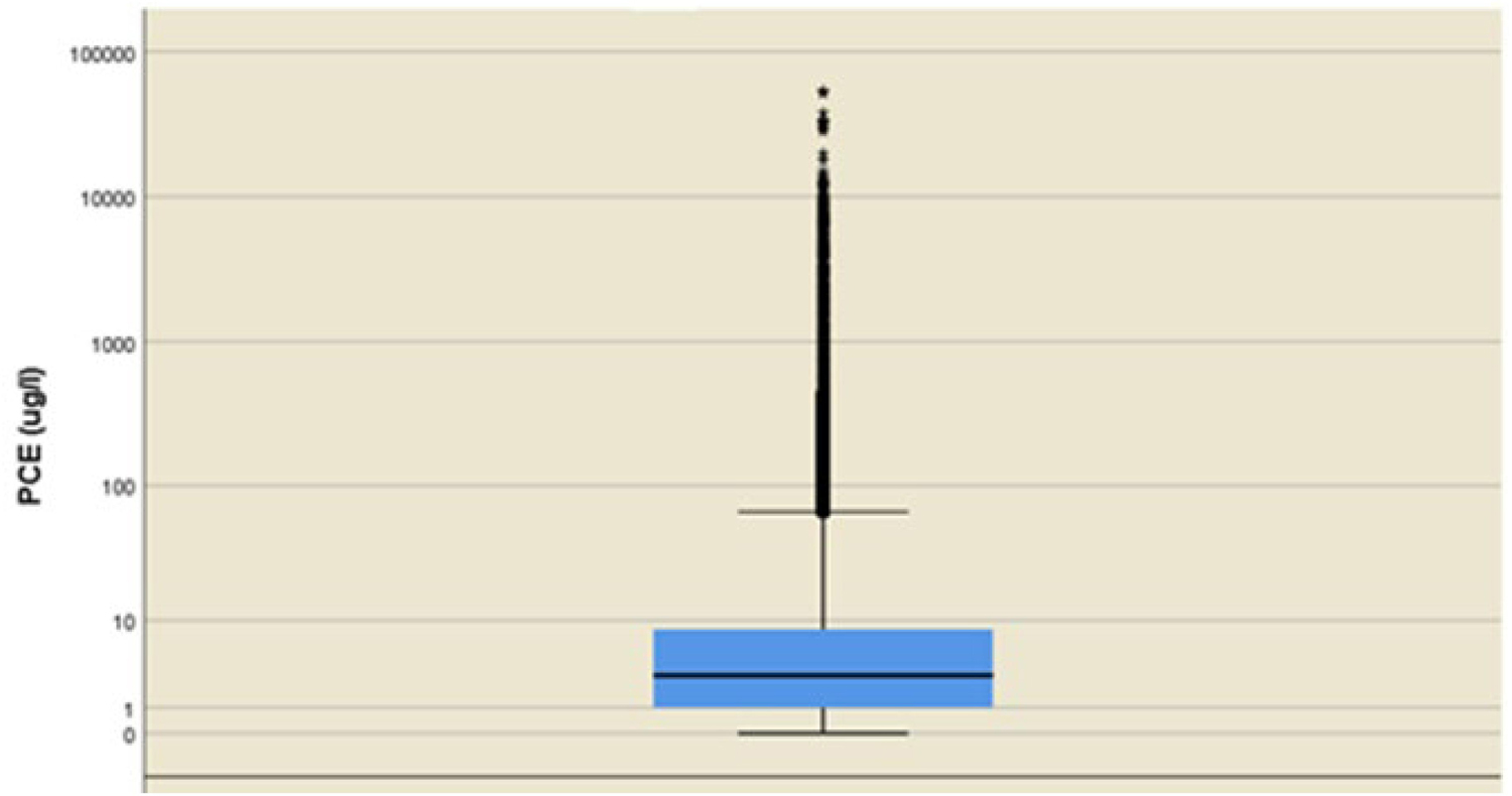
Figure 5. Boxplot in a logarithmic scale of the distribution of the 48,316 PCE measurements (μg/L). Mild outliers (i.e., points beyond the inner fences) are drawn as dots, whereas extreme outliers (i.e., points beyond the outer fences) are drawn as stars.
– lower inner fence: Q1 - 1.5∗IQ
– upper inner fence: Q3 + 1.5∗IQ
– lower outer fence: Q1 - 3∗IQ
– upper outer fence: Q3 + 3∗IQ
A point beyond an inner fence on either side is considered a mild outlier. A point beyond an outer fence is considered an extreme outlier.
Cluster analysis results are shown in Table 2, and Figure 6 displays the 15 clusters and their composition in terms of number of cases included. It can be observed that most of the clusters contain a very small amount of data, whereas a single cluster, number 1, contains 99% of the PCE values with concentrations considerably lower than the other clusters. The data belonging to this cluster 1 can be considered to define the DPBLs, whereas the other 14 clusters may be possibly attributed to hotspots (i.e., PSs).
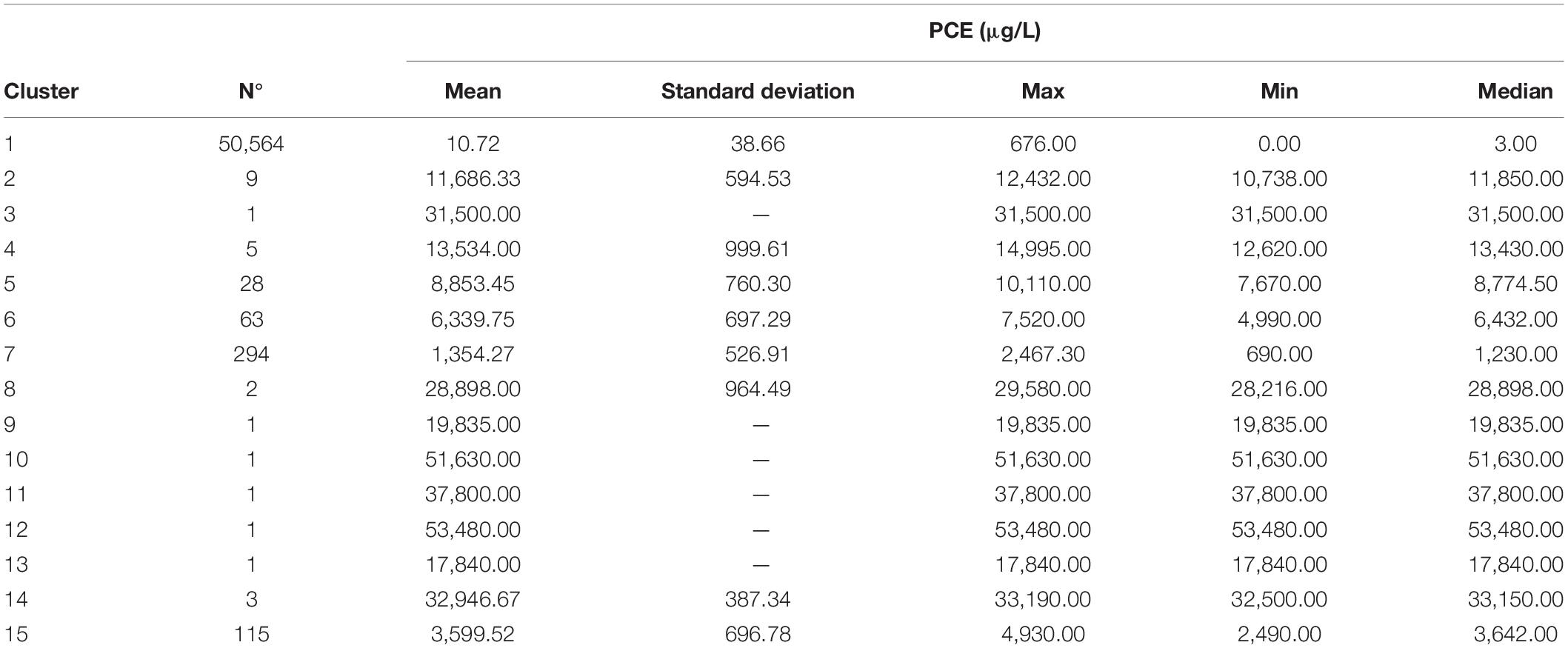
Table 2. The number of cases, frequencies, and summary statistics included in each of the 15 clusters.
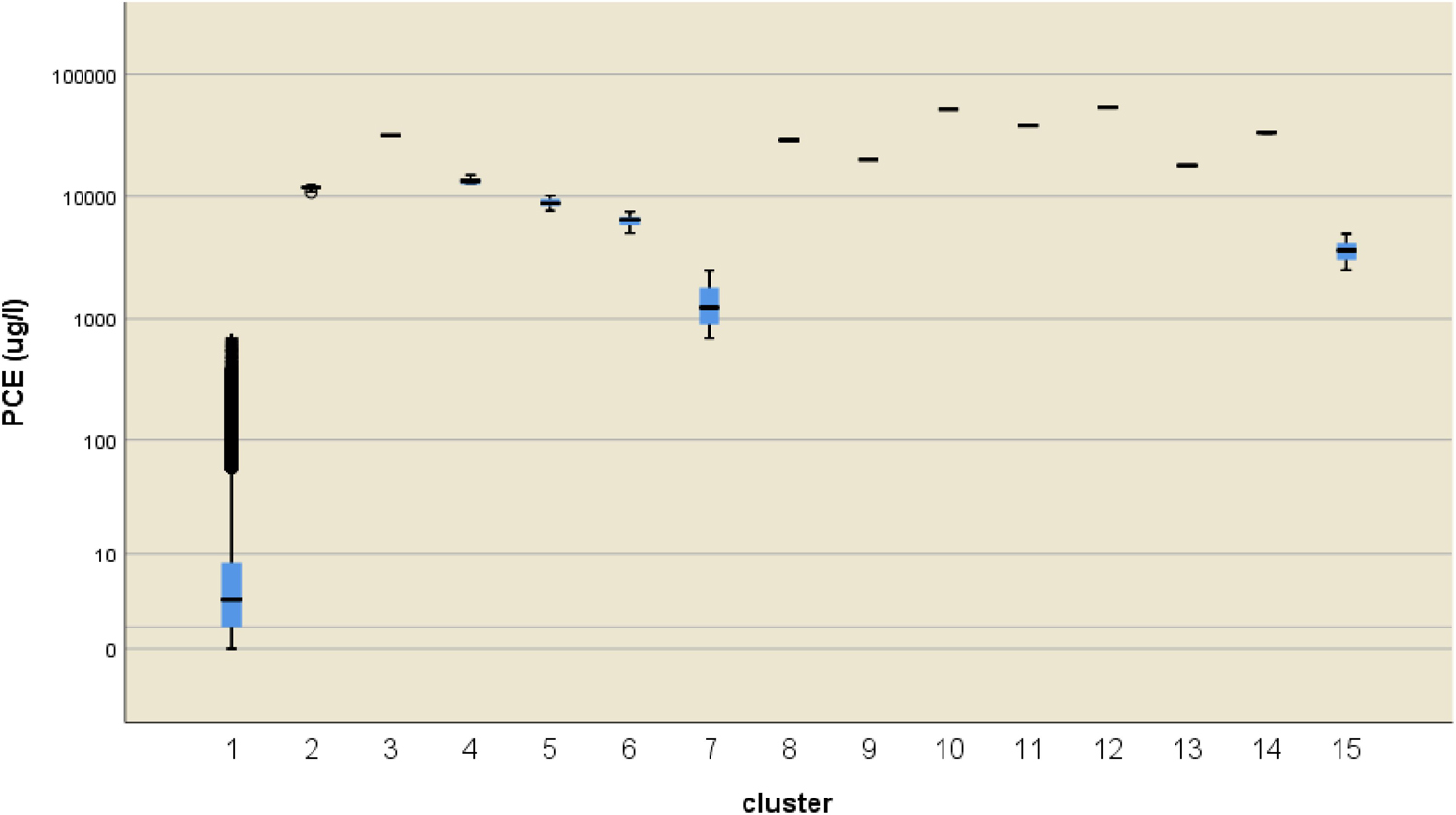
Figure 6. Representation of 15 clusters identified through CA using boxplots in a logarithmic scale for the PCE concentrations (μg/L).
By cross-checking the position of the monitoring points belonging to the smaller and extreme clusters with the information available from the AGISCO database (ARPA Lombardia, 2019), which contains the location of contaminated/potentially contaminated sites (remediated or in progress to be remediated, Figure 7), it was possible to identify which monitoring wells fell into a contaminated/potentially contaminated sites. Based on documental research (e.g., investigations, remediations, characterizations) for each of the interested site, it was possible to derive the history of the area and the temporal profile of the source, which was potentially linked to the sampled downgradient PCE contamination. Such a cross-check allowed to further subdivide the monitoring wells falling in the 14 smaller clusters as (1) point sources wells, when monitoring wells are inside the boundaries of the industrial site; (2) plumes wells in case of monitoring wells positioned downstream an industrial site and crossed by a contaminant plume; and (3) isolated wells, monitoring points without a clear association with a known potential industrial contaminant source, which might be affected by an “unknown source” (Figure 7). So, the CA was a fundamental tool that helped to identify (1) the cluster containing data with median values no higher than 4–5 μg/L and (2) the clusters made of outliers that were hotspots (i.e., PSs) and candidates as contaminated/potentially contaminated sites (PSs) to be simulated by the transport numerical model.
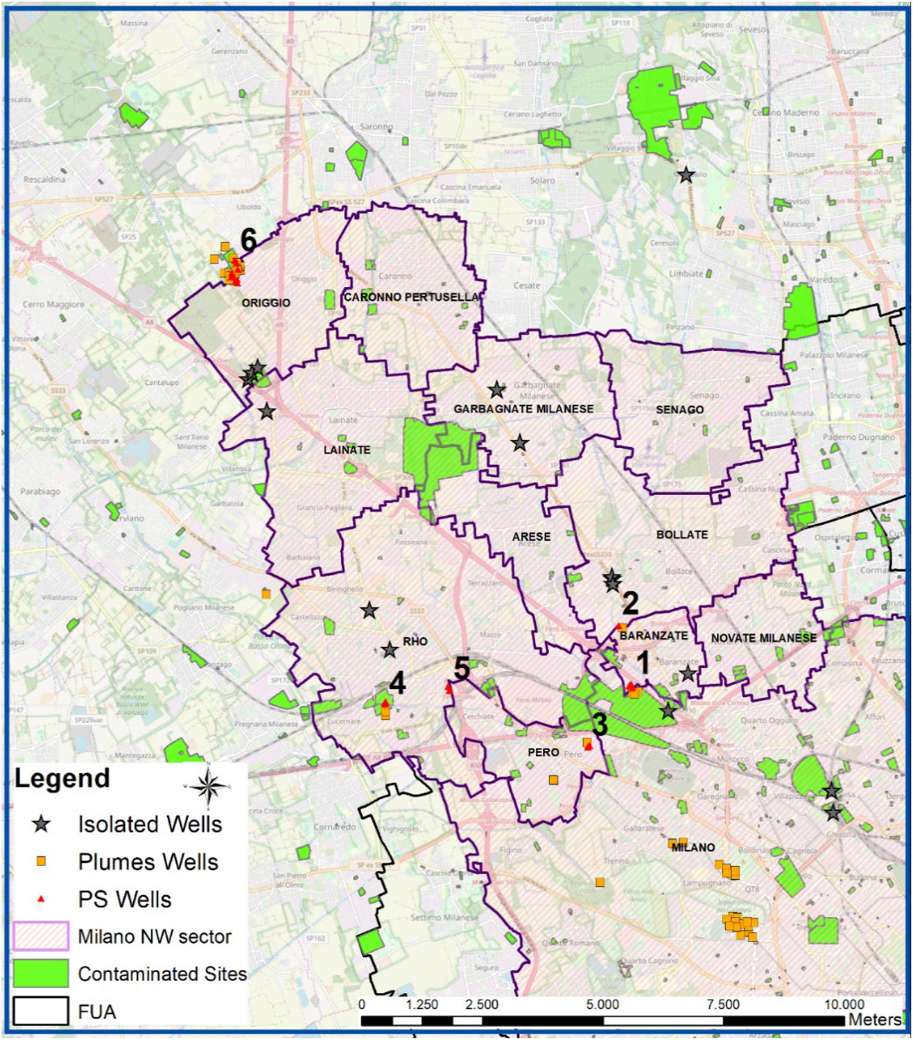
Figure 7. Monitoring wells belonging to clusters 2 to 15 overlapped with contaminated/potentially contaminated sites; numbered triangles correspond to PSs simulated in the transport model.
A 3D numerical transport model was implemented considering the previously identified PCE PSs as contaminant sources. In order to simulate the history of each source (numbered from 1 to 6 in the Figure 8), the modeled time interval started from 1955 until 2017. Thus, simulation stress periods were defined as 7:6 with a time interval of 10 years and one with a time interval of the 3 years (representing the period 2014–2017). In Figure 8, the 2017 contours of the PCE plumes originating from the main sources are shown (starting from 1955) concerning Aquifers A (Figure 8a) and B (Figure 8b). The transport model results were validated with the available data from 1955 to 2017 considering for each stress period the average concentration at each sampling point. The Italian Law threshold limit (IT-Decree 3/04/2006.n. 152, 2006) is 1.1 μg/L for PCE. Through a Geographical Information System (ArcGIS v.15), the plumes were overlapped to the monitoring network map, selecting all the points falling inside the isoconcentration line 1.1 μg/L. Then those points were excluded from the final dataset, which included only those monitoring points falling in white areas of Figure 8 that are not linked to any specific sources and can be considered affected only by a diffuse pollution. Furthermore, the numerical simulation confirmed that those monitoring points previously defined as Plume Wells are actually falling within the areas occupied by the plumes, validating the accuracy of the univariate CA results. Differently the points defined as Isolated Wells are not located in any of the simulated plumes. Because of the high concentrations of PCE and the fact that the univariate CA showed that they do not belong to cluster 1, it was assumed that such wells were affected by plumes due to unknown sources and consequently had to be deleted from the dataset used for the assessment of the PCE DPBL.
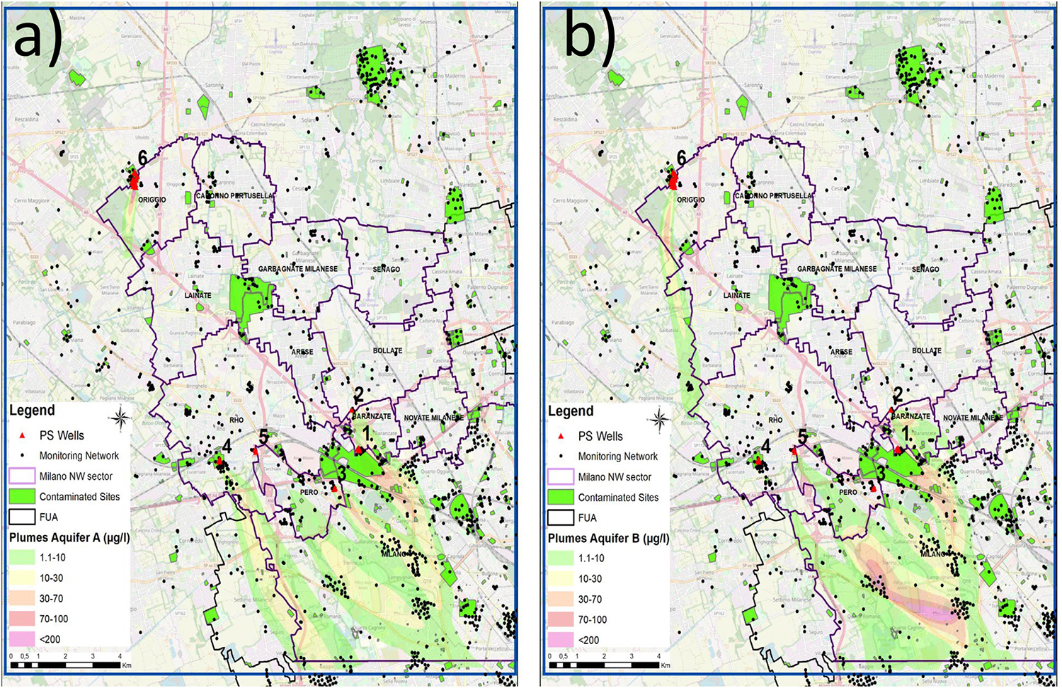
Figure 8. PS related plumes simulation selected by the CA in (a) the shallow aquifer and (b) the semiconfined aquifer.
Both the exploratory data analysis and the groundwater flow and transport model phases allowed to identify the monitoring points linked to some specific PSs and plumes. These monitoring points were later excluded from the following analysis. Thus, the spatial interpolation of the PCE 7-year median values allowed to identify different zones characterized by different levels of diffuse contamination in the NW sector of the Milano FUA. Figure 9a shows the shallow aquifer and the intersection between the monitoring points and plume areas delimited by the isoconcentration line of 1.1 μg/L (i.e., the EQS for PCE defined by the IT-Decree 3/04/2006.n. 152, 2006). Monitoring wells that had to be removed from the dataset are represented in black. In Figure 9b, only the median values of the diffuse pollution dataset that was used for the spatial interpolation is shown. For semiconfined Aquifer B, the corresponding maps are available in the Supplementary Figures S2, S3. The maps resulting from IDW interpolation of PCE median values are presented in Figures 9c,d, respectively, for the shallow and the semiconfined aquifer. In those maps, PCE concentration levels are subdivided into three different classes: (1) below the EQS, (2) between EQS and the drinking water threshold limit (i.e., 10 μg/L for the sum of PCE and TCE IT-Decree 3/03/2001.n. 31, 2001), and above the drinking water threshold limit. The maps clearly show that the distribution of diffuse contamination is not homogeneous within the study area. Areas in light blue are characterized by PCE concentrations below 1.1 μg/L, and thus, they are not affected by groundwater diffuse pollution. Areas in yellow show PCE concentrations exceeding the EQS but lower than the drinking water threshold limit and, finally, the red areas that reflect PCE concentrations higher than the drinking water threshold limit that are not attributable to a specific plume or source and are distributed over large areas. The use of IDW combined with multivariate analysis allowed also dealing with the high heterogeneity of the raw dataset (high density of sampled data is in the contaminated sites or in proximity to the Drinking Water Pumping Station).

Figure 9. (a) Intersection between the complete dataset and the 1.1 μg/L isoconcentration lines of the plumes for Aquifer A; (b) representation for the shallow aquifer of median values (period 2010–2017) of the adjusted dataset used to IDW interpolation process and (c) spatial map of the diffuse contamination in the shallow/unseparated aquifer and (d) in semiconfined Aquifer B.
Details about this analysis can be found in Azzellino et al. (2019). In short, PCA was applied to the groundwater parameters (Table 1) in order to select few factors (Fs) able to describe the whole dataset and the information useful for the definition of DPBLs in the different areas of the NW sector Milano FUA. Five rotated PCs were extracted and accounted for about 75% of cumulative variance from the original 12 variables. Table 3 shows the matrix of the factor loadings, which represent the correlation of each variable with each rotated PCs.
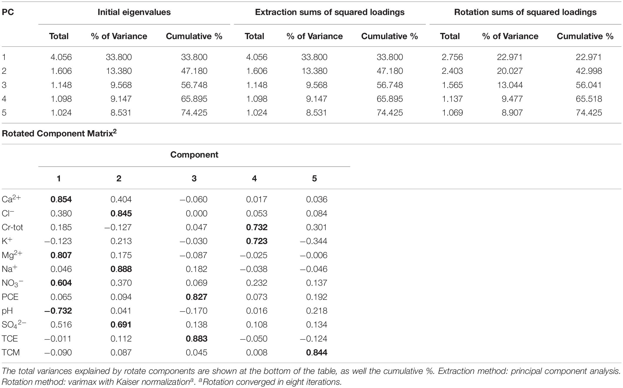
Table 3. Factor loading matrix: the loadings higher than | 0.6| are bolded and indicated as the significant loadings for the corresponding factor.
Based on factor loadings, the varifactors can be interpreted as follows:
• F1 accounts for 23% of the variance, and it is loaded by Ca2+, Mg2+, and NO3–. The correlation between Ca2+ and NO3– can be associated with the use of fertilizers, which is very common in cultivated regions, as in the studied area (Tisdale and Nelsson, 1975).
• F2 accounts for 20% of the variance and is loaded by Cl–, Na+, and SO42–, and it can be associated to the leakage of agricultural and municipal wastes (Sikora et al., 1976).
• F3 accounts for 13% of the variance and is loaded by PCE and TCE, which, in reason of their production, use, and chemical affinity, are often simultaneously found in groundwater.
• F4 accounts for 9.5% of the variance and is loaded by K+ and total chromium (Cr) that is another typical contaminant detected in Milano FUA groundwater. F5 accounts for 9% of the variance and is loaded by trichloromethane (TCM), which is also a chlorinated hydrocarbon largely used in industrial productions.
PCA/FA highlighted that chlorinated hydrocarbons (PCE-TCE) concentrations are correlated, being loaded on the same factor. Hydrochemical parameters are instead split into two different components (main ions in Table 3), whereas the other two dominant pollutants, Cr and TCM, are uncorrelated being, respectively, loaded on the fourth (i.e., 9.5% of the total variance) and on the fifth (i.e., 9% of the total variance) varifactor.
Based on these five factors, a new k-means CA was run in order to identify the different contamination profiles. In these clusters the varifactor F3 (e.g. loaded by PCE/TCE) is never higher than one standard deviation from the general sample mean. The parameter k was set to 15, and the analysis was run twice, using the final cluster centroids obtained from the first analysis as initial seeds for the second. This process, being based on multiple parameters, allowed to split further the cluster 1 previously obtained through the univariate CA and to better characterize the different patterns of diffuse contamination present in the study area. Five clusters, namely, 1, 6, 10, 11, and 15, contained more than 98% of the data (Supplementary Table S2). In these clusters, the varifactor F3 (e.g., loaded by PCE/TCE) is never higher than 1 standard deviation from the general sample mean (Figure 10). The main statistics of these five clusters are reported in Supplementary Table S1. The PCE concentration statistics of these clusters were used to estimate the DPBLs as reported in section “DPBL Definition.”
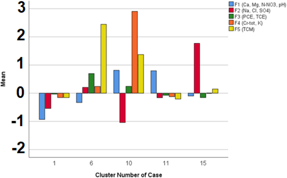
Figure 10. Varifactor characteristics of the main clusters: bars show the mean varifactor values of the main clusters. The reference scale on the y axis is the one of the standardized variables, so 0 is the total sample average, and 1 is the total sample standard deviation.
The results shown in previous paragraphs confirm that the Milano FUA cannot be managed as a homogeneous groundwater body. Five main diffuse pollution patterns were identified, with specific hydrogeological characteristics and pollutant background concentration levels. Therefore, considering both the lack of spatial homogeneity and the temporal variability observed in PCE levels, the estimation of the DPBLs was done based on the clusters and referred to the concentration classes (i.e., yellow zone and red zone showing PCE values higher than 1.1 μg/L). Since, because of the temporal variability, monitoring wells belonging to different clusters may fall in the same concentration class zone, DPBL was defined based on the clusters’ statistics weighted by the frequency of each of the five clusters in the two concentration class zones. For example, considering the yellow zones (i.e., PCE concentrations higher than 1.1 μg/L but lower than 10 μg/L) in the shallow aquifer, being the frequencies of the five main clusters, respectively, 0.0, 0.0, 20.0, 31.4, and 48.6%, based on the cluster statistics of PCE concentrations shown in Supplementary Table S1, the DPBL was computed as follows:
where Ci is the reference concentration, corresponding to 50° percentile of the specific cluster statistics (Supplementary Table S1) and fi (%) is the i-cluster frequency in the yellow concentration class zone. The same computation was carried out concerning the red zone (i.e., PCE concentration higher than 10 μg/L) as reported in Table 4.

Table 4. DPBLs ranges for PCE for the 2 separated Aquifers and the unseparated one in NW sector of Milano FUA.
In this study, a robust methodology was set up and tested considering the groundwater pollution problem in the Milano FUA. By using many different tools, through this methodology, it was possible to accurately identify specific background and threshold values that represent key information for the improvement groundwater management.
Previous studies have also used some of the tools we used in this work but never in such integrated way. Multivariate techniques have been applied in several studies for the assessment of groundwater quality, for the analysis of groundwater geochemistry and identification of sources (Reimann and Filzmoser, 2000; Yu et al., 2014; Acikel and Ekmekci, 2018; Adhikari and Mal, 2019; Stefania et al., 2019); numerical transport models have been applied for trace main plumes for management of groundwater, remediation, and mitigation strategies (El Bouqdaoui and Aachib, 2018; Colombo et al., 2019; Guo et al., 2019; Sathe and Mahanta, 2019; Janža et al., 2020); geostatistical analysis has been applied to map some environmental variables and contamination zoning (Guadagnini et al., 2020; Hossain and Patra, 2020). Moreover, previous works mainly focused on NBLs (Matschullat et al., 2000; Molinari et al., 2012; Ducci et al., 2016; Sellerino et al., 2019) of groundwater contaminants. In a previous study of this research (Azzellino et al., 2019), we posed the basis for a statistical approach to deal with diffuse contamination; in this work, the proposed methodology has been completed by adding the deterministic transport model to simulate the most relevant plumes deriving from a PS contamination in the FUA and to identify the subareas affected by these plumes that should be excluded from the geostatistical interpolation of the diffuse contamination.
This study has also shown that the PCE groundwater contamination within the NW sector of Milano FUA is present at different concentration levels with a heterogeneous spatial distribution. The methodology was able to separate the different contributes to this state of pollution: on one side due to PSs and their plumes and on the other due to MPSs responsible for a state of contamination that, despite being low, is diffused over a large part of FUA. This result has been reached combining univariate CA and transport numerical modeling. Such a modeling step may introduce some flaws in the methodology. It is known in fact that when transport modeling is applied in large areas with contaminated sites that have a long and complicated industrial history (e.g., brownfields, old landfills), uncertainties of the model results can be relevant. The suggestion in order to model the source as best as possible is to collect as much data as possible concerning the site characterization.
In this perspective, an overestimation of the plume dimension (length and width) would be preferable as it is possible to delete from the original dataset some monitoring wells that could be influenced by the PSs (i.e., some high concentration values that could overestimate the diffuse contamination estimation). Differently, leaving them in the analysis database, it would possibly lead to overestimating the concentrations obtained in the diffuse contamination interpolation maps. Furthermore, the choice to assume as diffuse contamination reference value, a weighted statistic based on the clusters’ frequency in the range between 50th and 75th percentiles, guarantees that the DPBLs are not be overestimated.
Defining appropriate DPBLs for the present contaminants is both a political and a scientific–technical issue. The case study presented in the article highlights that the Milano FUA is not a homogeneous groundwater body from the contamination perspective, and therefore, it is important to define different DPBLs within FUA subareas. Moreover, in order to take into account the spatial and temporal heterogeneity of the contamination, the clusters’ statistics, being robust and stable in time, were chosen to be the basis for defining DPBLs as the frequencies of each cluster rather than just the dominant were considered as representative of the concentration class zones.
Consequently, a unique value of DPBLs for the whole area was not defined, but different values for each concentrationclass zone and for each aquifer were provided (Table 4). Furthermore, a range for each DPBL was provided considering the 50th and 75th percentiles of the cluster concentration statistics. The definition of a range rather than a single reference value allows public authorities, responsible of the groundwater management plan, to take decisions and to undertake actions considering also political and administrative aspects. Indicatively, the use of 50th percentile is suggested for the yellow zones, while the use of the 75th percentile is suggested for the red zones.
In the future, in order to apply the proposed methodology in other urbanized areas, it would be useful to define minimum requirements about the density of monitoring wells and concentration data.
The definition of DPBLs is critical to select and optimize the remediation actions needed for the aquifer restoration, especially in areas where restoration goals might not be achieved because of a massive historical presence of unknown MPSs (characterized by small dimension and low mass release).
Recognizing the existence of a diffuse contamination and defining a specific threshold limit for each contaminant of interest (i.e., DPBLs) do not mean allowing polluters to contaminate or to avoid their responsibilities. Differently, it allows public and private decision-makers to understand whether a site is a source of pollution or is exposed to a diffuse contamination following the European Polluter Pay Principle. Consequently, it is possible to set appropriated and eventually new remediation objectives and to choose between different technical approaches for site clean-up, with efficiency and remediation times that vary substantially as a function of the associated costs and the environmental impact.
Many areas all around the world with a relevant industrialization history are affected by groundwater contamination. In the Milano FUA, where the groundwater was historically interested by PCE and TCE contaminations from both PSs (or hotspots, because of the presence of many factories and chemical plants) and MPSs from the surface (i.e., septic tanks or dry wells in industrial sites), a presence of many factories and chemical plants (i.e., automotive and galvanic) has also to be considered. In such large and complex urban area, characterized by the presence of shallow clustered MPSs (i.e., septic tanks, sewer leakages or dry wells) whose effects overlap with the plumes originated by specific PSs (or hotspots, e.g., leakages from petrochemical plants or factories), a multidisciplinary integrated approach is needed in order to quantify an anthropogenic DPBLs. In the EU legislative framework, there is no indication about how to define DPBLs, which in many situations are higher than the groundwater quality standards and make unfeasible any remediation strategy. The integrated methodological approach presented in this study has the objective to help managing FUAs, which are particularly large and affected by complex contamination patterns due to the high industrialization.
The use of statistical approach (PCA/FA) together with numerical model (MODFLOW/MT3DMS) allows distinguishing two components of pollution: the first linked to a specific source responsible for the main plumes that flew into Milano City and the second spread in the FUA as a diffused contamination. Because of the necessity to produce management plan of the area by the public authorities, the use of the main statistics of the clusters described in this study, applied to the zones outlined by the IDW interpolation, allowed to compute DPBLs for PCE in both the shallow Aquifer A and the semiconfined B. The methodology here presented would be applicable in every other FUA to quantify the non-homogeneous groundwater body quality in high industrialized and densely populated areas.
The data analyzed in this study is subject to the following licenses/restrictions: Data about contaminated sites are confidential due to ongoing legal procedures. Requests to access these datasets should be directed to Regione Lombardia through the online form: YW1iaWVudGVfY2xpbWFAcGVjLnJlZ2lvbmUubG9tYmFyZGlhLml0.
All authors: conceptualization and methodology, geostatistical analysis, and assessment of DPBLs. LC and AA: writing – original draft preparation. LA and MB: writing, review, editing, and supervision. LC and LA: modeling development. AA and LC: statistical analysis.
This study was performed within AMIIGA Project (Integrated Approach to Management of Groundwater Quality in Functional Urban Areas), financially supported by the program INTERREG Central Europe 2016–2019 – Grant CE N32.
The authors declare that the research was conducted in the absence of any commercial or financial relationships that could be construed as a potential conflict of interest.
We thank Regione Lombardia and Lombardy Environmental Protection Agency for providing the extensive available dataset of monitoring dataset and the full access to contaminated sites historical data. Moreover, we thank Water Managers for the data concerning the Pumping Wells Stations. Finally, we would like to acknowledge the reviewers who help us to improve the text and the quality of the manuscript.
The Supplementary Material for this article can be found online at: https://www.frontiersin.org/articles/10.3389/fenvs.2020.525469/full#supplementary-material
Acikel, S., and Ekmekci, M. (2018). Assessment of groundwater quality using multivariate statistical techniques in the Azmak Spring Zone, Mugla, Turkey. Environ. Earth Sci. 77:753. doi: 10.1007/s12665-018-7937-x
Adhikari, K., and Mal, U. (2019). Application of multivariate statistics in the analysis of groundwater geochemistry in and around the open cast coal mines of Barjora block, Bankura district, West Bengal, India. Environ. Earth Sci. 78:72. doi: 10.1007/s12665-019-8071-0
Afifi, A., May, S., and Clark, V. A. (2003). Cluster Analysis: Computer-Aided Multivariate Analysis. Boca Raton, FL: CRC Press.
Alamdar, R., Kumar, V., Moghtaderi, T., and Naghibi, S. J. (2019). Groundwater quality evaluation of Shiraz City, Iran using multivariate and geostatistical techniques Groundwater quality evaluation of Shiraz City, Iran using multivariate and geostatistical techniques. SN Appl. Sci. 1:1367. doi: 10.1007/s42452-019-1108-x
Alberti, L., and Francani, V. (2001). Studio idrogeologico sulle cause del sollevamento della falda nell’area milanese. Geoing. Ambient. Miner. 104, 257–264.
Alberti, L., Azzellino, A., Colombo, L., and Lombi, S. (2016a). “Use of cluster analysis to identify tetrachloroethylene pollution hotspots for the transport numerical model implementation in urban functional area of Milan, Italy,” in Proceedings of the International Multidisciplinary Scientific GeoConference Surveying Geology and Mining Ecology Management, SGEM, Albena.
Alberti, L., Cantone, M., Colombo, L., Lombi, S., and Piana, A. (2016b). Numerical modeling of regional groundwater flow in the Adda-Ticino Basin: advances and new results. Rend. Online Soc. Geol. Ital. 41:80. doi: 10.3301/ROL.2016.80
Alberti, L., Colombo, L., and Formentin, G. (2018). Null-space Monte Carlo particle tracking to assess groundwater PCE (Tetrachloroethene) diffuse pollution in north-eastern Milan functional urban area. Sci. Total Environ. 621, 326–339. doi: 10.1016/j.scitotenv.2017.11.253
Alderuccio, M., Cantarella, L., Ostoich, M., Ciuffi, P., Gattolin, M., Tomiato, L., et al. (2019). Identification of the operator responsible for the remediation of a contaminated site. Environ. Forens. 20, 339–358. doi: 10.1080/15275922.2019.1657521
ARPA Lombardia (2015). PROGETTO PLUMES: Final Report. Available online at: https://www.regione.lombardia.it/wps/portal/istituzionale/HP/DettaglioRedazionale/istituzione/direzioni-generali/direzione-generale-ambiente-e-clima/piano-per-inquinamento-diffuso
Azzellino, A., Colombo, L., Lombi, S., Marchesi, V., Piana, A., Merri, A., et al. (2019). Groundwater diffuse pollution in functional urban areas: the need to define anthropogenic diffuse pollution background levels. Sci. Total Environ. 656, 1207–1222. doi: 10.1016/j.scitotenv.2018.11.416
Balderacchi, M., Filippini, M., Gemitzi, A., KlÃve, B., Petitta, M., Trevisan, M., et al. (2014). Does groundwater protection in Europe require new EU-wide environmental quality standards? Front. Chem. 2:32. doi: 10.3389/fchem.2014.00032
Bini, A. (1997). Stratigraphy, chronology and palaeogeography of quaternary deposits of the area between the Ticino and Olona rivers (Italy-Switzerland). Geol. Insub. 2, 21–46.
Bortoni, S. F., Schlosser, R. T., and Barbosa, M. C. (2019). Numerical modeling of multiphase extraction (MPE) aiming at LNAPL recovery in tropical soils. Water 11:2248. doi: 10.3390/w11112248
Busico, G., Cuoco, E., Kazakis, N., Colombani, N., Mastrocicco, M., Tedesco, D., et al. (2018). Multivariate statistical analysis to characterize/discriminate between anthropogenic and geogenic trace elements occurrence in the Campania Plain, Southern Italy. Environ. Pollut. 234, 260–269. doi: 10.1016/j.envpol.2017.11.053
Carcano, C., and Piccin, A. (2002). Geologia degli acquiferi padani della Regione Lombardia. Soc. Elaborazioni Cartogr, Florence.
Cavallin, A., Francani, V., and Mazzarella, S. (1983). Studio Idrogeologico Della Pianura Compresa fra Adda e Ticino. Poland: La Fiaccola.
Cloutier, V., Lefebvre, R., Therrien, R., and Savard, M. M. (2008). Multivariate statistical analysis of geochemical data as indicative of the hydrogeochemical evolution of groundwater in a sedimentary rock aquifer system. J. Hydrol. 353, 294–313. doi: 10.1016/j.jhydrol.2008.02.015
Colombo, L., Alberti, L., Mazzon, P., and Formentin, G. (2019). Transient flow and transport modelling of an historical CHC source in North-West Milano. Water. 11:w11091745. doi: 10.3390/w11091745
Ducci, D., de Melo, M. T. C., Preziosi, E., Sellerino, M., Parrone, D., and Ribeiro, L. (2016). Combining natural background levels (NBLs) assessment with indicator kriging analysis to improve groundwater quality data interpretation and management. Sci. Total Environ. 569–570, 569–584. doi: 10.1016/j.scitotenv.2016.06.184
El Bouqdaoui, K., and Aachib, M. (2018). Delimitation of the perimeters of protection of groundwater catchments of the berrechid aquifer (Morocco) through hydrogeological modeling. J. Geosci. Environ. Protect. 6, 101–112. doi: 10.4236/gep.2018.67008
Erto, A., Andreozzi, R., Di Natale, F., Lancia, A., and Musmarra, D. (2009). “Experimental and isotherm-models analysis on TCE and PCE adsorption onto activated carbon,” in Proceedings of the 9th International Conference on Chemical and Process Engineering, New York, NY.
EU-Directive 2006/118/CE (2006). Groundwater directive 2006/118/CE: directive of the European parliament and of the Council on the protection of groundwater against pollution and deterioration. Off. J. Eur. Union 19, 19–31.
Guadagnini, L., Menafoglio, A., Sanchez-Vila, X., and Guadagnini, A. (2020). Probabilistic assessment of spatial heterogeneity of natural background concentrations in large-scale groundwater bodies through functional geostatistics. Sci. Total Environ. 740:140139. doi: 10.1016/j.scitotenv.2020.140139
Guo, Z., Fogg, G. E., Brusseau, M. L., LaBolle, E. M., and Lopez, J. (2019). Modeling groundwater contaminant transport in the presence of large heterogeneity: a case study comparing MT3D and RWhet. Hydrogeol. J. 27, 1363–1371. doi: 10.1007/s10040-019-01938-9
Harbaugh, A. W. (2005). MODFLOW-2005: The U S Geological Survey Modular Ground-Water Model — the Ground-Water Flow Process. Reston, VA: U.S. Geological Survey.
Hossain, M., and Patra, P. K. (2020). Contamination zoning and health risk assessment of trace elements in groundwater through geostatistical modelling. Ecotoxicol. Environ. Saf. 189:110038. doi: 10.1016/j.ecoenv.2019.110038
IT-Decree 3/03/2001.n. 31. (2001). Implementation of Directive 98/83/EC on the Quality of Water Intended for Human Consumption. G.U. della Repubblica Italiana n. 52, 3.03.2001, Italy.
IT-Decree 3/04/2006.n. 152 (2006). Norme in materia ambientale (Italian Environmental Codel -– IEC), O.J. n. 88 of 14/04/2006.
Janža, M., Prestor, J., Pestotnik, S., and Jamnik, B. (2020). Nitrogen mass balance and pressure impact model applied to an urban aquifer. Water 12:1171. doi: 10.3390/W12041171
La Vigna, F., Sbarbati, C., Bonfà, I., Martelli, S., Ticconi, L., Aleotti, L., et al. (2019). First survey on the occurrence of chlorinated solvents in groundwater of eastern sector of rome. Rend. Lincei. 30, 297–306. doi: 10.1007/s12210-019-00790-z
Matschullat, J., Ottenstein, R., and Reimann, C. (2000). Geochemical background - Can we calculate it? Environ. Geol. 39, 990–1000. doi: 10.1007/s002549900084
Molinari, A., Guadagnini, L., Marcaccio, M., and Guadagnini, A. (2012). Natural background levels and threshold values of chemical species in three large-scale groundwater bodies in Northern Italy. Sci. Total Environ. 425, 9–19. doi: 10.1016/j.scitotenv.2012.03.015
Olsen, R. L., Chappell, R. W., and Loftis, J. C. (2012). Water quality sample collection, data treatment and results presentation for principal components analysis e literature review and Illinois River watershed case study. Water Res. 46, 3110–3122. doi: 10.1016/j.watres.2012.03.028
Ostoich, M., Mason, L., Gattolin, M., Alderuccio, M., Cantarella, L., Cavinato, C., et al. (2019). Contamination of groundwater: obligations of non-responsible parties. Environ. Forens. 2019, 1–23. doi: 10.1080/15275922.2019.1657522
Parrone, D., Ghergo, S., and Preziosi, E. (2019). A multi-method approach for the assessment of natural background levels in groundwater. Sci. Total Environ. 659, 884–894. doi: 10.1016/j.scitotenv.2018.12.350
Perego, R., Bonomi, T., Fumagalli, M. L., Benastini, V., Aghib, F., Rotiroti, M., et al. (2014). 3D reconstruction of the multi-layer aquifer in a Po Plain area. Rend. Online Soc. Geol. Ital. 30, 41–44. doi: 10.3301/ROL.2014.09
Pereira, P. (2019). Soil Degradation, Restoration and Management in a Global Change Context, 1st Edn, Cambridge, MA: Academic Press.
Regione Lombardia (2017). Delimitazione Degli Areali Interessati da Inquinamento Diffuso da Tetracloroetilene, Tricloroetilene e Triclorometano Delle Acque Sotterranee dell ’area Vasta, Italy. Available online at: https://www.regione.lombardia.it/wps/portal/istituzionale/HP/DettaglioRedazionale/istituzione/direzioni-generali/direzione-generale-ambiente-e-clima/piano-per-inquinamento-diffuso
Reimann, C., and Filzmoser, P. (2000). Normal and lognormal data distribution in geochemistry: Death of a myth. Consequences for the statistical treatment of geochemical and environmental data. Environ. Geol. 39, 1001–1014. doi: 10.1007/s002549900081
Rotiroti, M., and Fumagalli, L. (2013). “Derivation of preliminary natural background levels for naturally Mn, Fe, As and NH4+ rich groundwater: the case study of Cremona area (Northern Italy),” in Proceedings of the Rendiconti Online Società Geologica Italiana, New York, NY.
Rotiroti, M., Di Mauro, B., Fumagalli, L., and Bonomi, T. (2015). COMPSEC, a new tool to derive natural background levels by the component separation approach: application in two different hydrogeological contexts in northern Italy. J. Geochemical Explor. 158, 44–54. doi: 10.1016/j.gexplo.2015.06.017
Sathe, S. S., and Mahanta, C. (2019). Groundwater flow and arsenic contamination transport modeling for a multi aquifer terrain: assessment and mitigation strategies. J. Environ. Manag. 231, 166–181. doi: 10.1016/j.jenvman.2018.08.057
Sellerino, M., Forte, G., and Ducci, D. (2019). Identification of the natural background levels in the Phlaegrean fields groundwater body (Southern Italy). J. Geochem. Explor. 200, 181–192. doi: 10.1016/j.gexplo.2019.02.007
Serianz, L., Cerar, S., and Šraj, M. (2020). Hydrogeochemical characterization and determination of natural background levels (NBL) in groundwater within the main lithological units in Slovenia. Environ. Earth Sci. 79:373. doi: 10.1007/s12665-020-09112-1
Sheikhy Narany, T., Ramli, M. F., Aris, A. Z., Sulaiman, W. N. A., and Fakharian, K. (2014). Spatiotemporal variation of groundwater quality using integrated multivariate statistical and geostatistical approaches in Amol-Babol Plain. Iran. Environ. Monit. Assess. 186, 5797–5815. doi: 10.1007/s10661-014-3820-8
Sikora, L., Bent, M., Corey, R., and Keeney, D. (1976). Septic nitrogen and phosphorus removal test system. Groundwater 14, 309–314. doi: 10.1111/j.1745-6584.1976.tb03120.x
Stefania, G. A., Rotiroti, M., Buerge, I. J., Zanotti, C., Nava, V., Leoni, B., et al. (2019). Identification of groundwater pollution sources in a landfill site using artificial sweeteners, multivariate analysis and transport modeling. Waste Manag. 95, 116–128. doi: 10.1016/j.wasman.2019.06.010
Stefania, G. A., Rotiroti, M., Fumagalli, L., Zanotti, C., and Bonomi, T. (2018). Numerical modeling of remediation scenarios of a groundwater Cr(VI) plume in an alpine valley aquifer. Geoscience 8:209. doi: 10.3390/geosciences8060209
Tisdale, S., and Nelsson, W. (1975). Soil Fertility and Fertilizers. New York, NY: Macmillan Publishing Co Inc.
Wang, Q., Song, X., Tang, S., and Yu, L. (2020). Enhanced removal of tetrachloroethylene from aqueous solutions by biodegradation coupled with nZVI modified by layered double hydroxide. Chemosphere 243:125260. doi: 10.1016/j.chemosphere.2019.125260
Watson, D. F., and Philip, G. M. (1985). A refinement of inverse ditance weighted interpolation. Geo Process. 2, 315–327.
Watts, R. J., and Teel, A. L. (2019). Hydroxyl radical and non-hydroxyl radical pathways for trichloroethylene and perchloroethylene degradation in catalyzed H2O2 propagation systems. Water Res. 38, 5465–5469. doi: 10.1016/j.watres.2019.05.001
Yidana, S. M., Ophori, D., and Banoeng-Yakubo, B. (2008). A multivariate statistical analysis of surface water chemistry data-The Ankobra Basin, Ghana. J. Environ. Manag. 86, 80–87. doi: 10.1016/j.jenvman.2006.11.023
Yu, Y., Song, X., Zhang, Y., Zheng, F., Liang, J., and Liu, L. (2014). Identifying spatio-temporal variation and controlling factors of chemistry in groundwater and river water recharged by reclaimed water at Huai River, North China. Stoch. Environ. Res. Risk Assess. 28, 1135–1145. doi: 10.1007/s00477-013-0803-1
Zheng, C. (2010). MT3DMS v5.3 Supplemental User’s Guide. Department of Geological Sciences, University of Alabama, Tuscaloosa, Alabama, 1–56.
Keywords: transport model, FUA, cluster analysis (CA), multivariate analysis, DPBLs, diffuse contamination, Milan
Citation: Colombo L, Alberti L, Azzellino A and Bellotti M (2020) Multi-Methodological Integrated Approach for the Assessment of Diffuse Pollution Background Levels (DPBLs) in Functional Urban Areas: The PCE Case in Milano NW Sector. Front. Environ. Sci. 8:525469. doi: 10.3389/fenvs.2020.525469
Received: 09 January 2020; Accepted: 07 September 2020;
Published: 16 October 2020.
Edited by:
Andrew Hursthouse, University of the West of Scotland, United KingdomReviewed by:
Mitja Janža, Geological Survey Ljubljana, SloveniaCopyright © 2020 Colombo, Alberti, Azzellino and Bellotti. This is an open-access article distributed under the terms of the Creative Commons Attribution License (CC BY). The use, distribution or reproduction in other forums is permitted, provided the original author(s) and the copyright owner(s) are credited and that the original publication in this journal is cited, in accordance with accepted academic practice. No use, distribution or reproduction is permitted which does not comply with these terms.
*Correspondence: Loris Colombo, bG9yaXMuY29sb21ib0Bwb2xpbWkuaXQ=
†These authors have contributed equally to this work
Disclaimer: All claims expressed in this article are solely those of the authors and do not necessarily represent those of their affiliated organizations, or those of the publisher, the editors and the reviewers. Any product that may be evaluated in this article or claim that may be made by its manufacturer is not guaranteed or endorsed by the publisher.
Research integrity at Frontiers

Learn more about the work of our research integrity team to safeguard the quality of each article we publish.