An Alternative Approach for Deriving Emission Inventories Solely From Satellite Data: Demonstration for NO2 Over China

We demonstrate an alternative method for deriving of emission estimates for pollutants using solely columnar satellite data. The method, which we term Lifetime-Modified Accumulation Method (LMAM), does not require any ancillary model run or other data to estimate emissions, but needs only the measured columnar amounts. It employs lifetime calculations from measured daily columnar amounts. The method is applied to nitrogen dioxide over China on a 0.25 × 0.25 and a 1× 1° grid, and emission estimates are derived and compared with a more traditional method. The emission estimates thus derived appear to be consistent with traditional methods, both in their spatial distribution and their magnitude, and correlate well with existing inventories. Ways for refining the method are discussed. The method can be improved, we only wanted to demonstrate here it is feasible to derive inventories solely from satellite data using lifetime calculations.

Introduction

Emission inventories of air pollutants are necessary for modeling and formulation of abatement policies. Usually, inventories are compiled bottom-up, using statistics on activities emitting and their typical emission factors. Many steps in this process are associated with uncertainties that can be large. Additionally, the compilation is time consuming thus making frequent updates tiresome. Inventories can be also compiled top-down, using satellite observations. This latter approach has several advantages over the former, as being spatially consistent, having better temporal resolution, and being more frequently updateable at a fraction of the cost.

Especially for emissions of south-east Asia, especially China, which exhibit rapidly evolving trends (e.g., van der A et al., 2006, 2008; Kourtidis et al., 2018; Sogacheva et al., 2018; Georgoulias et al., 2019), top-down emission inventories from satellite observations are very appealing. Since satellites measure concentrations and not emissions, alongside satellite observations a Chemistry-Transport-Model (CTM) or some other tool needs to be applied, to calculate an emission inventory from columnar amount fields. Information for adjusting the model emissions is contained in the difference between observed and modeled fields. Due to transport, this inversion problem becomes computationally complex.

In recent years, a variety of studies involving application of different techniques, addressed estimates of NOx emissions from satellite observations (see Mijling and van der A, 2012 and references therein). Some studies dealt also with emission calculations of NOx from megacities (Beirle et al., 2011), and, more recently, emissions from individual sources (Fioletov et al., 2011, 2013, 2015).

Spatial emission inventories using satellite data to date require alongside the satellite observations the application of a CTM. Very recently, a method was presented that can derive emissions for one pollutant from its relationship with another pollutant whose emissions are known (Kourtidis et al., 2018). Here, we present a method for the calculation of spatial inventories of pollutants that requires only satellite columnar data and does not require the additional involvement of a CTM or another pollutant with known emissions.

Materials and Methods

In this work, daily gridded tropospheric NO₂ data for 2007 at a spatial resolution of 0.25 × 0.25° were used from the Ozone Monitoring Instrument (OMI) aboard EOS Aura satellite. The NO₂ concentration data (10¹⁵ molecules/cm²) are part of the OMNO2d v3 dataset (Krotkov, 2013; Krotkov et al., 2017). The OMNO2d data are compiled using clear sky retrievals (cloud fraction <30%). In addition, daily gridded wind velocity data from the ECMWF Re-Analysis (ERA)-Interim (Dee et al., 2011) are used. The data were produced by the Integrated Forecast System (IFS) of the ECMWF (European Center for Medium-Range Weather Forecasts) at a native horizontal resolution of ~79 km assimilating satellite and in-situ observations. The ERA-Interim data were downscaled to the satellite data grid by applying bilinear interpolation.

The basics for the Lifetime-Modified Accumulation Method (LMAM) are described below.

The method requires three steps for implementation. The first step, is the calculation of the lifetime of the species under investigation, the second the exclusion of well-ventilated grid boxes for each day, and the last the emission calculation.

In the beginning, the timeseries of daily observations in each grid is calculated. The calculation of lifetime is based on the work of Junge (1974), who observed that the relative standard deviation (standard deviation divided by the mean mixing ratio) of the mixing ratio of long-lived species was inversely proportional to their atmospheric lifetime τ. According to this work, the lifetimes of atmospheric species are τ = 0.14 [X_mean]/σ([X]) with τ in years. Subsequent experimental and theoretical works (e.g., Jobson et al., 1998, 1999; Williams et al., 2000; Lenschow and Gurarie, 2002; Becker et al., 2009), have shown that other relationships might apply, depending on the lifetime range and other factors, as the airmass age and the location of sources. These relationships might be of the form σ(ln[X]) = A τ^−b. For very long-lived species, which exhibit small variability, σ(ln[X]) is equivalent to the relative standard deviation and Junge's relationship might be applied. A is a fitting parameter determined in the regression and being interpreted as a measure of the range of air mass ages in the sampled data, as determined by the time period between emission and measurement. A is having low values (down to 0.99) for small ranges of ages and higher values (up to 4.63) for datasets with wide range of ages (Jobson et al., 1999; Williams et al., 2000). The exponent b has a value between 0 and 1, being an indicator of the relative strength of sink terms and turbulent mixing upwind of the measurement location, where higher values signify the dominance of chemical loss processes. Values of b = 0.18 (Williams et al., 2000) signify relative fresh emissions whereas values near 0.5 correspond to well-aged emissions. A relationship σ(ln[X]) = 0.99 τ^−0.18 with τ in days appears to apply for a wide range of lifetimes, 1.5–500 days, which gives σ(lnX) = 0.85 for τ = 1.5 days (Jobson et al., 1999).

Estimating nitrogen dioxide emissions from satellite data has progressed quite during the last decade, hence we decided to apply the LMAM method for NO₂ so that we can compare it with a mature inventory as DECSO (Daily Emission estimates Constrained by Satellite Observations). NOx satellite-based emission estimates from KNMI's DECSO algorithm (Mijling and van der A, 2012; Mijling et al., 2013; Ding et al., 2017) were used. More specifically, DECSO v1, v3a, and v5.1 monthly data, which were constructed using OMI/Aura measurements, were used. The DECSO v1 and DECSO v3a relative error is ~35% for the monthly mean emissions used here (Kourtidis et al., 2018). The corresponding precision for the DECSO v5 emissions is ~20% (Ding et al., 2017).

Results and Discussion

For the application of the LMAM method we proceeded as follows: In the first step the lifetime of NO₂ was calculated. We made two calculations, one for the simple Junge (1974) relationship τ = 0.14 [NO_2mean]/σ([NO₂]) and one from the equation σ(ln[NO₂]) = τ^−0.18, which applies for a wide range of lifetimes (Jobson et al., 1999) and which solved for τ gives τ = (1/σ{ln[NO₂]})^(1/0.18). These results are presented in Figure 1. We note here that the very high lifetimes calculated over certain regions of China, especially the south, can have two origins: cloud cover is higher over Southern China and has a seasonal nature (e.g., Pan et al., 2016) due to monsoons, hence there is artificially less variability in the retrievals. Further, mean NO₂ concentrations are low in regions with increased lifetime calculations, hence more retrievals will be below detection, which will also induce artificially less variability in the retrieved concentrations.

FIGURE 1

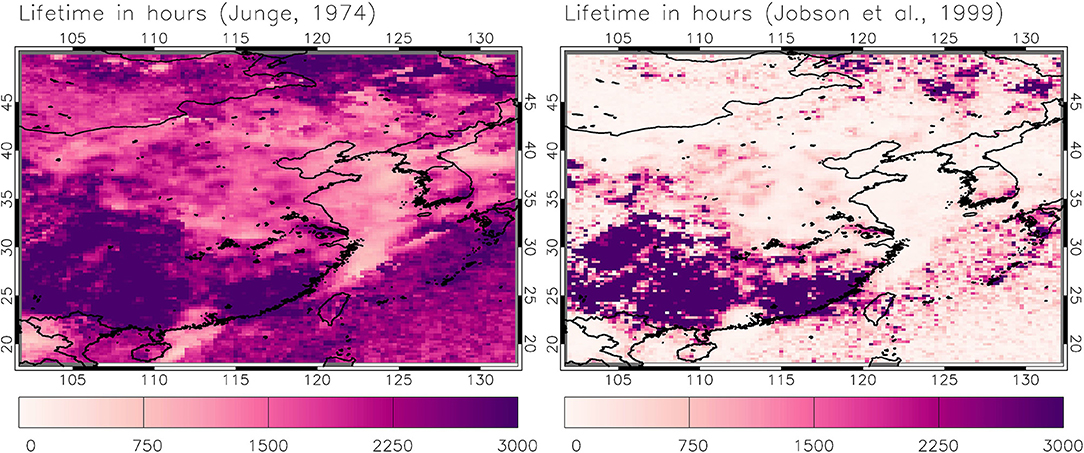
Figure 1. Left: NO₂ lifetime τ for 2007 calculated from τ = 0.14 [NO_2mean]/σ[NO₂], where [NO_2mean] is the average yearly OMI Tropospheric NO₂ column (in 10¹⁵ molec/cm²) and σ[NO₂] is the standard deviation of the daily values. Right: NO₂ lifetime τ for 2007 calculated from the σ(ln[NO₂]) = τ^−0.18 equation. The map axes are in degrees Eastern longitude/Northern latitude.

In the second step, we try to exclude well-ventilated boxes, to avoid, as far as possible, smearing of the calculations due to entrainment of emissions from nearby grid boxes. We made two calculations, one with a 0.25 × 0.25° and one with 1 × 1° grid, the latter corresponding to roughly 100 × 100 km at the southernmost of the study region and 70 × 70 km at the northernmost. Here, we made the following assumptions: The contents of the box are ventilated by the horizontal wind within time t_vent which might be approximated by t_vent = L/wv (in hours), where L is the length of the box in km and wv is the wind velocity in km/h. So our grid boxes will need more than 3 or 12 h, respectively, to be ventilated completely for wind speeds lower than 2 m/s. Given the fact that the atmospheric lifetime of NO₂ will range between an order of magnitude lower than the ventilation time (in summer) and the same order of magnitude as the ventilation time (in winter), that the majority of wind speeds were <2 m/s and also the fact that the NO₂ retrievals are many more in summer (due to less cloud cover) than the winter, we assumed for the demonstration here that the effect of ventilation in the lifetime calculation will not be very great if we exclude only wv ≥4 m/s.

For the last step in the calculation we assume that for the air pollutant under investigation (e.g., NO₂ in our case), its lifetime τ in respect to physicochemical removal within the particular grid box is equal to τ (in hours), and its emission rate is M (in kg/h). The lifetime is here the e-folding time or half-life, i.e., the time required for the removal of half of the pollutant. Assuming that at a given concentration point, the concentration of the pollutant, i.e., NO₂, within the box without horizontal ventilation, will reach equilibrium, i.e., its physicochemical removal rate will equal its emission rate, we will have:

$\begin{array}{ll}\text{d}\left[\text{N}{\text{O}}_2\right]/\text{dt }=\text{ M}-\text{λ}\left[\text{N}{\text{O}}_2\right]=0,& (1)\end{array}$

where λ is the NO₂ removal rate, which is related to its lifetime τ through λ = 1/[τ ln(2)] and M is the emission rate.

From (1) we have, after substituting λ = 1/[τ ln(2)] = 1/(0.693 τ) in M = λ[NO₂], we get M = [NO₂]/(0.693 τ) = 1.44[NO₂]/τ. Since [NO₂] is known from satellite observations, if τ can be calculated, we can infer the emission rate M as M = C^*1.44[NO2]/τ, where C is a correction factor (C = 10). The correction factor is applied to account for two effects, namely: (1) "Local source effects”, which will “significantly suppress variability of reactive species” and result in higher τ calculations (Jobson et al., 1998) and hence lower emission rates M. (2) Accounting for the seasonal lifetime changes, since τ was calculated from yearly data. Average ratios of summer to winter σ(lnx) values may be around 1.5 for species with lifetimes in the range 1–500 days (Jobson et al., 1999), which is consistent with the Goldstein et al. (1995) estimated factor of 10 seasonal change in lifetime given the observed τ^−0.18 dependence (Jobson et al., 1999).

The method shows very good agreement with DECSO in the spatial distribution, except for the areas over sea where emissions appear relatively high as compared with the land ones (Figure 2). This reflects the fact that lifetimes are calculated lower over sea, due to three facts: Firstly, variability is higher over the sea because of worse retrieval quality and daily fluctuations in ship traffic. Secondly, within the ship plumes, elevated levels of NOx lead to enhanced levels of OH during the day, enhanced levels of NO₃ and N₂O₅ at night, and hence reduced lifetimes (Davis et al., 2001). Thirdly, variability in ship traffic and tracks can artificially lead to increased variability in concentrations which in turn will impact lifetime calculations (Becker et al., 2009) and thus emission calculations. For the area of study, our method calculates average emissions (averaged over all cells, in 10¹⁵ molecules/cm²/h) of 0.0026 (with lifetimes calculated after Junge (1974), i.e., with τ = 0.14 [NO_2mean]/σ([NO₂], figure not shown) and 0.2548 (with lifetimes calculated after Jobson et al. (1999), i.e., with τ = (1/σ{ln[NO₂]})^(1/0.18), while DECSO calculates average emissions of 0.3746 (v1), 0.364 (v3a) and 0.2663 (v5.1). As expected, calculating lifetimes after Junge (1974), yields unrealistically high lifetimes and hence unrealistically low emissions. Calculating lifetimes after Jobson et al. (1999), yields average emissions, which compare very well with DECSO v5.1 (the difference being around +4%, much lower than the error of DECSO v5.1 which is ~20%). The spatial agreement with DECSO of the approach we presented here is also quite well (Figure 2). On the 0.25 ×0.25° grid cell level, on a % basis, our emissions are within the DECSO v5.1 ~20% error in 32% of the cells. On an absolute values basis, using a 0.25 × 0.25° grid, in 82% of the grid boxes differences with DECSO v5.1 are less than 0.5 (10¹⁵ molecules/cm²/h). For a larger 1 × 1° grid, this happens in 87% of the grid boxes, most probably as a result of longer grid box ventilation times. Given that the differences between the first DECSO v1 and the last one DECSO v5.1 are comparable, since for the 0.25 × 0.25° grid, in 91% of the grid boxes DECSO v1-DECSO v5.1 differences are <0.5 (10¹⁵ molecules/cm²/h), we believe we have presented here an approach that if refined further appears promising.

FIGURE 2

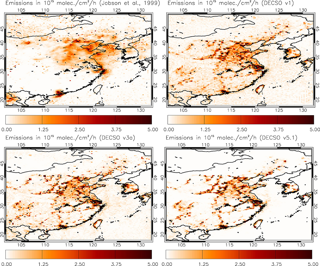
Figure 2. Emission estimates for 2007 from lifetime (τ) calculations from OMI daily data after Jobson et al. (1999) (see text), where τ = (1/σ{ln[NO₂]})^(1/0.18) (upper left) compared with DECSO v1 NOx emissions (upper right), DECSO v3a NOx emissions (lower left) and DECSO v5.1 NOx emissions (lower right). The map axes are in degrees Eastern longitude/Northern latitude.

We note here that NOx and NO₂ emission rates are not equal and may vary over time and space, however, one can reasonably assume that at polluted regions with high O₃ concentrations around noon (which is the OMI overpass time), which is the case over China, NOx/NO₂ rations will be around 1.28–1.30 (e.g., Seinfeld and Pandis, 2006; Jöckel et al., 2016), i.e., NOx will be actually about 28–30% more than NO₂. Such a ratio has been used in other NOx emission studies based on satellite NO₂ (Beirle et al., 2011; Liu et al., 2016). We have not dealt explicitly with this 30% correction here since it was out of the scope of the paper, which is simply a demonstration of feasibility.

Improvements can be achieved e.g., by:

After the first calculation of gridded emissions, use wind velocity and direction data and the gridded emission calculations to calculate transported amounts TR_IN and TR_OUT and then account for transport in Equation (1) d[NO₂]/dt = M–λ[NO₂] = 0 by modifying to

$\begin{array}{ll}\text{d}\left[\text{N}{\text{O}}_2\right]/\text{dt }=\text{ M}-\text{λ}\left[\text{N}{\text{O}}_2\right]+\text{ T}{\text{R}}_{\text{IN}}-\text{ T}{\text{R}}_{\text{OUT}}=0& (2)\end{array}$

Recalculate using M = TR_OUT−YR_IN+[NO₂]/(1.44 τ) and reiterate several times until no differences between calculation(n) and calculation (n−1) are observed.

Also, the use of another expression of the more general form σ(ln[X]) = A τ^−b (e.g., Jobson et al., 1998, 1999; Williams et al., 2000; Lenschow and Gurarie, 2002; Becker et al., 2009) instead of the simpler σ(ln[X]) = τ^−0.18 used here might be more appropriate. To determine the appropriate A and b coefficients, more theoretical work is needed. Also, has been shown that variability in long-term monitoring can be influenced by many factors which impacts the application of Junge type relations for lifetime calculations (Becker et al., 2009). Applying the Becker et al. (2009) arguments for NO₂, these can be large retrieval errors for columns near the detection limit, sources that release non-periodically as a result of a specific activity (as, e.g., ship traffic), seasonality, and random non-periodic events such as loss mechanisms variability and changes in wind. Theoretical work is also needed in addressing these factors and the suppression of their impact to lifetime calculations.

Conclusions

In view of the current interest in using satellite data for calculating emissions, as well as the future need to monitor greenhouse gas country emission allocations, we demonstrated here that it appears feasible to calculate gridded emissions from satellite data alone using lifetime calculations. In this first study of this nature, derived emissions appear to be consistent with traditional methods in their spatial distribution and magnitude. Over the whole domain of China, the difference in average emissions between our approach and DECSO v5.1 is around +4%. At its current formulation, the method has limited applicability in places where cloud cover is seasonally high, large number of retrievals is near the detection limit, or have sources that release non-periodically as a result of a specific activity, as, e.g., ship traffic. Ways of improving the method are outlined.

Data Availability Statement

The NO₂ satellite data analyzed in this work can be found on NASA's GES DISC Mirador website (http://mirador.gsfc.nasa.gov), the ERA-Interim reanalysis data can be found on ECMWF's website (www.ecmwf.int) and the KNMI DECSO emission data can be found on www.globemission.eu. The emission data that were generated for this study may be available upon request from the contact author.

Author Contributions

KK developed the theoretical basis for the LMAM method and wrote the largest part of the manuscript. AG performed the numerical calculations and wrote parts of the manuscript.

Funding

This research has been financed partly under the FP7 Programme MarcoPolo (Grant Number 606953, Theme SPA.2013.3.2-01) and partly under the Ministry of Economy and Development (Operational Programme Competitiveness, Enterpreneurship and Innovation - EPAnEK) ≪Panhellenic infrastructure for atmospheric composition and climate change (PANACEA)≫ Programme (MIS code 5021516).

Conflict of Interest

The authors declare that the research was conducted in the absence of any commercial or financial relationships that could be construed as a potential conflict of interest.

Acknowledgments

The authors acknowledge the use of satellite data from NASA's GES DISC Mirador website (http://mirador.gsfc.nasa.gov). The satellite data were acquired as part of the activities of NASA's Science Mission Directorate, and are archived and distributed by the Goddard Earth Sciences (GES) Data and Information Services Center (DISC). The authors acknowledge the use of KNMI DECSO emission data from www.globemission.eu and express their gratitude to ECMWF (www.ecmwf.int) for making available the ERA-Interim reanalysis data.

References

Becker, S., Halsall, C. J., Macleod, M., Scheringer, M., Jones, K. C., and Hungerbuehler, K. (2009). Empirical investigation of the junge variability-lifetime relationship using long-term monitoring data on polychlorinated biphenyl concentrations in air. Environ. Sci. Technol. 43, 2746–2752. doi: 10.1021/es900336y

PubMed Abstract | CrossRef Full Text | Google Scholar

Beirle, S. F., Boersma, K., Platt, U., Lawrence, M. G., and Wagner, T. (2011). Megacity emissions and lifetimes of nitrogen oxides probed from space. Science 333:1737. doi: 10.1126/science.1207824

PubMed Abstract | CrossRef Full Text | Google Scholar

Davis, D. D., Grodzinsky, G., Kasibhatla, P., Crawford, J., Chen, G., Liu, S., et al. (2001). Sandholm: impact of ship emissions on marine boundary layer NOx and SO₂ distributions over the Pacific Basin. Geophys. Res. Lett. 28, 235–238. doi: 10.1029/2000GL012013

CrossRef Full Text | Google Scholar

Dee, D. P., Uppala, S. M., Simmons, A. J., Berrisford, P., Poli, P., Kobayashi, S., et al. (2011). The ERA-Interim reanalysis: configuration and performance of the data assimilation system. Q. J. R. Meteorol. Soc. 137, 553–597. doi: 10.1002/qj.828

CrossRef Full Text | Google Scholar

Ding, J., van der A, R. J., Mijling, B., and Levelt, P. F. (2017). Space-based NOx emission estimates over remote regions improved in DECSO. Atmos. Meas. Tech. 10, 925–938. doi: 10.5194/amt-10-925-2017

CrossRef Full Text | Google Scholar

Fioletov, V. E., McLinden, C. A., Krotkov, N., and Li, C. (2015). Lifetimes and emissions of SO₂ from point sources estimated from OMI. Geophys. Res. Lett. 42, 1969–1976. doi: 10.1002/2015GL063148

CrossRef Full Text | Google Scholar

Fioletov, V. E., McLinden, C. A., Krotkov, N., Moran, M. D., and Yang, K. (2011). Estimation of SO₂ emissions using OMI retrievals. Geophys. Res. Lett. 38:L21811. doi: 10.1029/2011GL049402

CrossRef Full Text | Google Scholar

Fioletov, V. E., McLinden, C. A., Krotkov, N., Yang, K., Loyola, D. G., Valks, P., et al. (2013). Application of OMI, SCIAMACHY, and GOME-2 satellite SO₂ retrievals for detection of large emission sources. J. Geophys. Res. Atmos. 118, 11399–11418. doi: 10.1002/jgrd.50826

CrossRef Full Text | Google Scholar

Georgoulias, A. K., van der A, R. J., Stammes, P., Boersma, K. F., and Eskes, H. J. (2019). Trends and trend reversal detection in 2 decades of tropospheric NO2 satellite observations. Atmos. Chem. Phys. 19, 6269–6294. doi: 10.5194/acp-19-6269-2019

CrossRef Full Text | Google Scholar

Goldstein, H., Wofsy, S. C., and Spivakovsky, C. M. (1995). Seasonal variations of nonmethane hydrocarbons in rural New England: constraints on OH concentrations in northern mid latitudes. J. Geophys. Res. 100, 21023–21033. doi: 10.1029/95JD02034

CrossRef Full Text | Google Scholar

Jobson, B. T., McKeen, S. A., Parrish, D. D., Fehsenfeld, F. C., Blake, D. R., Goldstein, A. H., et al. (1999). Trace gas mixing ratio variability versus lifetime in the troposphere and stratosphere: observations. J. Geophys. Res. 104, 16090–16113. doi: 10.1029/1999JD900126

CrossRef Full Text | Google Scholar

Jobson, B. T., Parrish, D. D., Goldan, P., Kuster, W., Fehsenfeld, F. C., Blake, D. R., et al. (1998). Spatial and temporal variability of nonmethane hydrocarbon mixing ratios and their relation to photochemical lifetime. J. Geophys. Res. 103, 13557–13567. doi: 10.1029/97JD01715

CrossRef Full Text | Google Scholar

Jöckel, P., Tost, H., Pozzer, A., Kunze, M., Kirner, O., Brenninkmeijer, C. A. M., et al. (2016). Earth system chemistry integrated modelling (ESCiMo) with the modular earth submodel system (MESSy, version 2.51). Geosci. Model Dev. 9, 1153–1200. doi: 10.5194/gmd-9-1153-2016

CrossRef Full Text | Google Scholar

Junge, C. E. (1974). Residence time and variability of tropospheric trace gases. Tellus 26:477. doi: 10.3402/tellusa.v26i4.9853

CrossRef Full Text | Google Scholar

Kourtidis, K., Georgoulias, A. K., Mijling, B., van der A, R. J., Zhang, Q., and Ding, J. (2018). A new method for deriving trace gas emission inventories from satellite observations: the case of SO₂ over China. Sci. Total Environ. 612, 923–930. doi: 10.1016/j.scitotenv.2017.08.313

PubMed Abstract | CrossRef Full Text | Google Scholar

Krotkov, N. A. (2013). OMI/Aura NO₂ Cloud-screened Total and Tropospheric Column Daily L3 Global 0.25deg Lat/Lon Grid, Version 003. NASA Goddard Space Flight Center. Available online at: http://dx.doi.org/10.5067/Aura/OMI/DATA3007 (accessed February 25, 2019).

Google Scholar

Krotkov, N. A., Lamsal, L. N., Celarier, E. A., Swartz, W. H., Marchenko, S. V., Bucsela, E. J., et al. (2017). The version 3 OMI NO₂ standard product. Atmos. Meas. Tech. 10, 3133–3149. doi: 10.5194/amt-10-3133-2017

CrossRef Full Text | Google Scholar

Lenschow, D. H., and Gurarie, D. (2002). A simple model for relating concentrations and fluctuations of trace reactive species to their lifetimes in the atmosphere. J. Geophys. Res. 107:D24,4805. doi: 10.1029/2002JD002526

CrossRef Full Text | Google Scholar

Liu, F., Beirle, S., Zhang, Q., Dörner, S., He, K., and Wagner, T. (2016). NOx lifetimes and emissions of cities and power plants in polluted background estimated by satellite observations. Atmos. Chem. Phys. 16, 5283–5298. doi: 10.5194/acp-16-5283-2016

CrossRef Full Text | Google Scholar

Mijling, B., and van der A, R. J. (2012). Using daily satellite observations to estimate emissions of short-lived air pollutants on a mesoscopic scale. J. Geophys. Res. 117:D17302. doi: 10.1029/2012JD017817

CrossRef Full Text | Google Scholar

Mijling, B., van der A, R. J., and Zhang, Q. (2013). Regional nitrogen oxides emission trends in East Asia observed from space. Atmos. Chem. Phys. 13, 12003–12012. doi: 10.5194/acp-13-12003-2013

CrossRef Full Text | Google Scholar

Pan, Z., Mao, F., Gong, W., Wang, W., and Yang, J. (2016). Observation of clouds macrophysical characteristics in China by CALIPSO. J. Appl. Rem. Sens. 10:036028. doi: 10.1117/1.JRS.10.036028

CrossRef Full Text | Google Scholar

Seinfeld, J. H., and Pandis, S. N. (2006). Atmospheric Chemistry and Physics: From Air Pollution to Climate Change. New York, NY: John Wiley and Sons.

Google Scholar

Sogacheva, L., Rodriguez, E., Kolmonen, P., Virtanen, T. H., Saponaro, G., de Leeuw, et al. (2018). Spatial and seasonal variations of aerosols over China from two decades of multi-satellite observations—Part 2: AOD time series for 1995–2017 combined from ATSR ADV and MODIS C6.1 and AOD tendency estimations. Atmos. Chem. Phys. 18, 16631–16652. doi: 10.5194/acp-18-16631-2018

CrossRef Full Text | Google Scholar

van der A, R. J., Eskes, H. J., Boersma, K. F., van Noije, T. P. C., Van Roozendael, M., Smedt, ID., et al. (2008). Identification of NO₂ sources and their trends from space using seasonal variability analyses. J. Geophys. Res. 113:D04302. doi: 10.1029/2007JD009021

CrossRef Full Text | Google Scholar

van der A, R. J., Peters, D. H., Eskes, H., Boersma, K. F., Van Roozendael, M., Smedt, ID., et al. (2006). Detection of the trend and seasonal variation in tropospheric NO₂ over China. J. Geophys. Res. 111:D12317. doi: 10.1029/2005JD006594

CrossRef Full Text | Google Scholar

Williams, J., Fischer, H., Harris, G. W., Crutzen, P. J., Hoer, P., Hansel, A., et al. (2000). Variability-lifetime relationship for organic trace gases: a novel aid to compound identification and estimation of HO concentrations. J. Geophys. Res. 105, 20473–20486. doi: 10.1029/2000JD900203

CrossRef Full Text | Google Scholar