How Land Cover Spatial Resolution Affects Mapping of Urban Ecosystem Service Flows

Rioux, Jean-François; Cimon-Morin, Jérôme; Pellerin, Stéphanie; Alard, Didier; Poulin, Monique

doi:10.3389/fenvs.2019.00093

ORIGINAL RESEARCH article

Front. Environ. Sci., 25 June 2019

Sec. Land Use Dynamics

Volume 7 - 2019 | https://doi.org/10.3389/fenvs.2019.00093

This article is part of the Research Topic Assessment and Modeling of Soil Functions or Soil-Based Ecosystem Services: Theory and Applications to Practical Problems View all 12 articles

How Land Cover Spatial Resolution Affects Mapping of Urban Ecosystem Service Flows

$\nJean-Franois Rioux,$ Jean-François Rioux^1,2

Jérôme Cimon-Morin^1,2

Stéphanie Pellerin^2,3

Didier Alard^1,4

Monique Poulin^1,2^*

¹Département de Phytologie, Université Laval, Québec, QC, Canada
²Quebec Centre for Biodiversity Science, McGill University, Montréal, QC, Canada
³Institut de Recherche en Biologie Végétale, Université de Montréal and Jardin Botanique de Montréal, Montréal, QC, Canada
⁴UMR BIOGECO, Université de Bordeaux, INRA, Pessac, France

In urban areas, estimating the effect of land cover (LC) data spatial resolution on ecosystem services (ES) mapping remains a challenge. In particular, mapping spatial flows of ES, from greenspaces to beneficiaries, may be more sensitive to LC data resolution than mapping potential supply or demand separately. Our objectives were to compare the sensitivity of global- and local-flow ES maps to LC data resolution, and to assess the effect of LC data resolution within different types of urban land uses. A case study was conducted in the city of Laval, Canada. Carbon storage (a global-flow ES), urban cooling and pollination (two local-flow ES) were mapped using LC data aggregated from 1 to 15 m. Results were analyzed for districts (comprising various types of urban land uses), and for 480 × 480m residential and commercial zones. Greenspace cover was generally underestimated at coarser spatial resolutions; as a result, so were ES potential supply and flow. For urban cooling and pollination, the effect of LC data spatial resolution on ES flow also depended on changes in the spatial configuration of ES potential supply relative to ES demand. The magnitude of the effect differed among land use types. However, the effect was also highly variable between similar landscapes, suggesting that it is very sensitive to LC structure. To adequately map the ES provided by the small greenspaces scattered throughout the urban matrix, using land cover data with a spatial resolution of 5m or finer is recommended, especially for local-flow ES.

Introduction

Urban greenspaces provide several ecosystem services (ES), such as recreation, runoff mitigation and air cooling or purification, that contribute to citizens' security, health and quality of life (Bolund and Hunhammar, 1999; Tratalos et al., 2007; Bowler et al., 2010; Gomez-Baggethun and Barton, 2013; Irvine et al., 2013; Mexia et al., 2018). In this regard, a recent review on the economic value of urban greenspaces concluded that the flow of benefits largely surpass the management costs of these infrastructures (Tempesta, 2015). For example, the value of air pollution removal by urban trees in the United States has been estimated at $3.8 billion annually (Nowak et al., 2006), with $9.2 million for the city of Chicago alone (McPherson et al., 1997). In California, urban trees reduce peak energy load by 10%, resulting in annual savings of $779 million (McPherson and Simpson, 2003). Considering that two-thirds of the world's population is expected to live in cities by 2050 (United Nations, 2015), the role of urban greenspaces is unequivocal, especially since economic studies have demonstrated their efficiency.

There is a growing interest worldwide in integrating ES to guide urban planning with the aim of increasing the well-being (quality of life) of city dwellers (Gomez-Baggethun et al., 2013). To this end, ES mapping represents a useful tool (Pulighe et al., 2016). Yet, ES mapping is still an evolving field and the diversity of methods and data in use can produce divergent estimates of the amount and location of a given ES in the landscape (Crossman et al., 2013; Schulp et al., 2014; Bagstad et al., 2018). Accordingly, there is often a high level of uncertainty about the accuracy of the maps produced, which is seldom assessed (Hou et al., 2013; Boerema et al., 2017; Ochoa and Urbina-Cardona, 2017). One of the challenges is to develop a better understanding of these sources of uncertainty (Hamel and Bryant, 2017), in order to adapt the choice of methods and data to the objective of mapping (Schroter et al., 2015).

Land cover (LC) maps describing the biophysical characteristics of the land surface are one of the most common data sources used in ES mapping (Martínez-Harms and Balvanera, 2012). The spatial resolution of the data is an important feature of LC maps that has been shown to influence ES mapping, but the magnitude of the effect was found to vary depending on the ES and the landscape under study (Konarska et al., 2002; Schulp and Alkemade, 2011; Grêt-Regamey et al., 2014; Grafius et al., 2016; Bagstad et al., 2018; Zhao and Sander, 2018). For example, when mapping urban ES using 5 and 25 m resolution LC data, Grafius et al. (2016) estimated 1.3 times more carbon storage but 2.8 times less potential sediment erosion at the finer resolution. In another study, ES value for the conterminous United States was three times higher when calculated using 30 m LC data compared to 1 km data, but the magnitude of the difference varied between states (Konarska et al., 2002). Estimating the effect of LC data resolution on a given ES in a given landscape thus remains a challenge.

Part of the difficulty lies in estimating the effect of spatial resolution on the LC map itself. While the general effect of decreasing the spatial resolution of a LC map is an increase in the area of dominant classes at the expanse of rarer classes and a loss of information on fine-scale spatial heterogeneity (Turner et al., 1989; Wu, 2004), the precise changes depend on the actual structure of the landscape represented. For example, the effect of decreasing spatial resolution on the proportion of a LC class on a map depends on the proportion of this class in the landscape, the size of its patches and its level of clumpiness (Moody and Woodcock, 1995). Another part of the challenge is to relate changes in the LC map to the spatial processes involved in mapping the ES. In particular, spatially explicit ES models were found to be highly sensitive to LC data resolution in spatially heterogeneous environments (Schulp and Alkemade, 2011; Grafius et al., 2016; Bagstad et al., 2018).

For urban areas that are characterized by fine-scale spatial heterogeneity (Small, 2003; Cadenasso et al., 2007), the differences between very fine and coarser resolution urban LC maps may have a significant effect on urban ES mapping. This effect will also likely vary within the urban area as a function of land use (LU), which refers to the function to which a land parcel is dedicated. For example, the effect may be more pronounced in fine-grained, highly heterogeneous residential areas than in coarse-grained, more homogeneous commercial ones (Herold et al., 2002; Zhao and Sander, 2018). Advanced technology allows the production of urban LC maps with a very fine (i.e., ≤1 m) resolution (e.g., Zhou and Troy, 2008). Yet, such fine resolution LC maps are not readily available for all locations (Gong et al., 2019), and the resources needed to produce them may not be affordable for every ES mapping project, especially in low-income countries and outside academic institutions. When available, detailed maps often need to be aggregated to coarser resolution, due, amongst several reasons, to computational limitations or constraints on integrating them with other datasets (Raj et al., 2013). A better understanding of the effect of LC data spatial resolution on fine-scale urban ES mapping is thus needed to weigh the cost of investing in fine resolution LC maps against their benefits.

The high demand for ES in urban areas (Gomez-Baggethun and Barton, 2013) makes it important to understand the effect of LC data resolution on mapping not only ES supply, but also spatial flows of ES, i.e., the actual delivery of ES from greenspaces to beneficiaries (Villamagna et al., 2013; Haase et al., 2014). Spatial flows of ES result from the spatial relationship between the supply of ES and the demand for this ES, and can take different forms (Serna-Chavez et al., 2014). While some ES like wild fruit picking must be performed (used) in situ (spatial congruence of ES supply and demand), most ES are used at some distance from greenspaces. There is thus a spatial discrepancy between ES supply and beneficiaries. In particular, global-flow ES, like carbon storage, are totally independent of beneficiaries' location relative to the area of service production, while local-flow ES, like urban cooling, depend on the proximity between beneficiaries and greenspaces (Cimon-Morin et al., 2014; Cimon-Morin and Poulin, 2018). The effect of LC data spatial resolution on those two scales of spatial flows of ES may thus be different. Land use planning based solely on ES supply may not be adequate for ensuring that ES benefits are provided where beneficiaries need them and where these benefits can sustain their well-being (Cimon-Morin and Poulin, 2018). Yet, as most cities worldwide will continue to grow (Seto et al., 2011), mapping ES flow will be increasingly important for urban planners and decision makers in the years to come. This will require a comprehensive understanding of the relation between ES supply and demand (i.e., ES fluxes) and how spatial resolution of LC maps can modulate this relationship.

The aim of this study is therefore to provide empirical results that shed light on the effect of LC data spatial resolution on the three components of fine-scale urban ES mapping, which are supply, demand and flow. To this end, we documented the magnitude of the differences in LC structure and ES quantity between maps produced using LC data aggregated from 1 to 15 m, for a typical North American city. Three ES representing different scales of spatial flows were compared: carbon storage, a global-flow ES, as well as urban cooling and pollination, two local-flow ES. Results were analyzed for two levels of landscapes: large urban districts, and 480 ×480 m residential and commercial zones. Analysis at the district level aimed to assess the global effect of spatial resolution in the urban area, as districts were assumed to capture the overall heterogeneity of the urban landscape. Analysis at the level of residential and commercial zones aimed to assess the local effect of spatial resolution, as each LU type was assumed to exhibit a specific LC structure (Herold et al., 2002; Van de Voorde et al., 2011) and thus a specific scaling behavior. These two levels of analysis were used to better assess the variability of the effect of LC data resolution within the urban area.

Data and methods

Study Area

We conducted our study in Laval, a city located in southern Québec, Canada (Figure 1) with a land area of 247 km² and a population of 422,993 inhabitants in 2016 (Statistics Canada, 2016). Laval is part of Greater Montreal, Canada's second most populous metropolitan area. Originally an agricultural territory, the city has experienced accelerated urban sprawl since the 1950s (Nazarnia et al., 2016). Its form of development, typical of North American suburbs, is characterized by spatial segregation of uses, with extensive low-density residential and commercial areas intersected by a road network designed for automobile travel (Dupras et al., 2016; Nazarnia et al., 2016; Ville de Laval, 2017b). Yet, agricultural lands still occupy about a third of Laval's territory, mainly in the east.

FIGURE 1

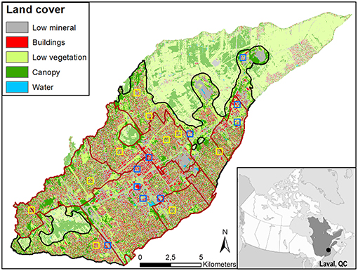
Figure 1. Location and land cover map of the study area. The land cover map also shows the delineation of the urban area in black, urban districts in dark red, residential zones in yellow, and commercial zones in blue. Land cover data source: Communauté Métropolitaine de Montréal (2017).

Land Cover Data

We used an existing 1 m spatial resolution raster land cover (LC) map of Laval's entire territory (Communauté Métropolitaine de Montréal, 2017). This map was created using color-infrared orthophotos taken in August 2015. Four LC classes were distinguished based on the normalized difference vegetation index (NDVI) and height: low mineral (NDVI < 0.3; height < 3 m), buildings (NDVI < 0.3; height > 3 m), low vegetation (NDVI > 0.3; height < 3 m) and tree canopy (hereafter referred to as “canopy”) (NDVI > 0.3; height > 3 m). A fifth class corresponding to water was added from ancillary data; however, as it covered only a small proportion of the study area (<1%), we treated it as a background class for the remainder of the study. Visual analysis of the original LC map revealed some systematic classification errors related to agricultural fields, water bodies and buildings that were corrected in a data preparation step (see Supplementary Material for more information on these corrections, as well as other methodological details).

The corrected 1 m LC map (Figure 1) was then aggregated to spatial resolutions of 3, 5, 10, and 15 m following a majority rule. To do so, the raster map was first converted to vector format, keeping the edges of the polygons the same as the raster's cell edge. This vector map was then converted back to rasters of coarser resolution using the “maximum combined area” cell assignment type in ArcMap (ESRI, 2015), so that the dominant LC class (the class covering the most extensive area) within a cell was assigned to this cell. In case of a tie between two LC classes, the cell was randomly assigned to one of the two.

Selection of Landscapes

Urban Districts

Since the focus of this study was on the urban landscape, urban areas of the territory had to be distinguished from the rural portions, which represented one third. Yet, there is no standard or universal definition of what constitutes an urban area (McIntyre et al., 2000; Raciti et al., 2012; Short Gianotti et al., 2016), as urbanization represents a multidimensional phenomenon (Hahs and McDonnell, 2006). A pragmatic solution to this issue is to develop and use a clearly-described working definition, adapted to the objective of the study (McIntyre et al., 2000).

Considering that surface imperviousness is a characteristic feature of urban areas (Hahs and McDonnell, 2006), the following LC based method was used to delineate and select urban districts in a quantitative and reproducible way, adapted from Raciti et al. (2012). It involved reclassifying the LC map into “impervious surfaces” (low mineral and buildings) and “greenspaces” (low vegetation and canopy). This reclassified map was used to calculate the impervious surface area in a 500 m radius moving window around each cell. A 15% imperviousness threshold was used to distinguish between urban (≥15%) and non-urban (<15%) cells. After testing many combinations of radius sizes and imperviousness percentages, the combination 500 m radius/15% imperviousness was chosen because it represented the best balance between cohesion in the urban area and distinction between urban and agricultural land uses. In addition, a radius of 500 m or less is often used in urban ecology to study the effects of the surrounding matrix on urban ecosystems (e.g., Coutts et al., 2007; Petralli et al., 2014; Schütz and Schulze, 2015; Melliger et al., 2018).

The 14 districts of Laval (Ville de Laval, 2017a) were then clipped to the urban area. The result of this operation corresponded to the “urban districts” as defined in this study. Urban districts too small or irregular in shape as a result of the clipping operation were excluded from the analysis. In the end, eight urban districts were selected for the analysis (Figure 1). These urban districts varied in size from about 3 to 40 km², and were all composed of a heterogeneous mix of different LU types.

Residential and Commercial Zones

In addition to these large heterogeneous urban districts, zones homogeneous in terms of land use (LU) were selected using an existing LU map (Communauté Métropolitaine de Montréal, 2016) that was reclassified into three broad LU types: residential, commercial (including commercial, industrial and office workplaces) and “other” (including every other LU, for example, parks, agricultural lands, the highway network and vacant lots). From a grid composed of 480 × 480 m polygons positioned over the urban area, two sets comprising the 25 polygons with the highest proportion of residential or commercial area were selected. For both residential and commercial sets of 25 polygons, 10 non-contiguous polygons were randomly chosen, which represent the 10 zones of analysis for each LU type (Figure 1).

Ecosystem Services Mapping

Conceptual Framework

Based on the conceptual framework proposed by Villamagna et al. (2013), our ecosystem services (ES) mapping method identified three components: potential supply, demand, and flow. ES potential supply refers to the “ecosystem's capacity to deliver services based on biophysical properties”; ES demand refers to “the amount of a service required or desired by society”; and ES flow refers to “the actual use of the service.” From a spatial perspective, an ES flow can be viewed as the spatial connection between the area of service production (provisioning area) and the area of service use by beneficiaries (benefiting area). For each provisioning area, the area within which the ES can potentially be used is defined as the flow area (Serna-Chavez et al., 2014). The presence of beneficiaries (expressing a demand) in the flow area gives rise to the actual ES flow.

Figure 2 illustrates how we applied these concepts in our mapping method. A distinctive feature of the method is that provisioning and benefiting areas were allocated to individual raster cells, while the flow area corresponded to a circular radius in and around each provisioning cell. A potential supply value was first attributed to every provisioning cell. This potential supply was then redistributed to every cell in the flow area around the provisioning cell. Doing so for every provisioning cell on the map determined the total potential supply received by each cell. A binary demand value of 1 (for model simplicity) was then attributed to each benefiting cell on the map, and a null value was assigned to other cells. Finally, the demand map was multiplied by the potential supply map to produce the flow map (Watson et al., 2019). In other words, the ES flows were quantified as the amount of supply received by each benefiting cell.

FIGURE 2

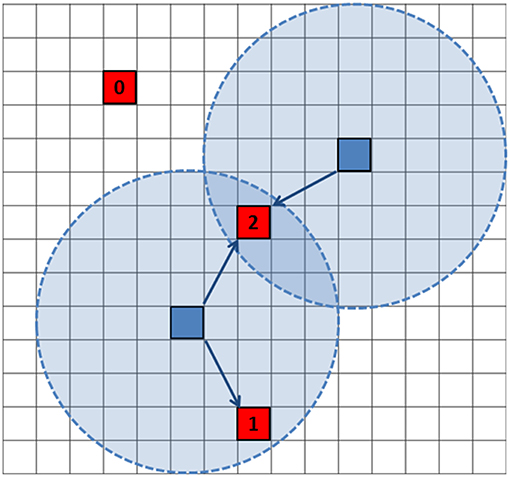
Figure 2. Illustration of the ecosystem services mapping method used. The figure depicts provisioning area as blue cells, benefiting area as red cells, flow area as transparent blue circles and ecosystem service flow as blue arrows. Ecosystem service flow is mapped as supplied to benefiting cells, and is quantified as the amount of supply received by a benefiting cell (numbers shown).

ES Selection and Mapping

The effect of LC data resolution was compared for two scales of spatial flows of ES: global-flow ES, which is independent of beneficiaries' location relative to provisioning areas, and local-flow ES, which depends on the proximity between provisioning and benefiting areas. Three ES were selected: (1) carbon storage, a global-flow ES; (2) urban cooling and (3) pollination, which are two local-flow ES. These three ES were mapped using simple models, and the five LC maps at different resolutions were used as input data. More complex models were not necessary to map ES for the purpose of our study, but would be needed to make concrete management decisions (Eigenbrod et al., 2010).

Carbon storage

The carbon storage model corresponded to global climate regulation by carbon storage in live biomass (Weissert et al., 2014). Based on data from the literature, a carbon storage value of 7.69 kgC/m² was attributed to canopy (Nowak et al., 2013), 0.22 kgC/m² to low vegetation (Jo and Mcpherson, 1995) and zero to impervious surfaces. As a global-flow ES, the flow area of carbon storage is the entire planet: carbon storage at any location contributes to global climate regulation. Therefore, all the carbon stored in the study area benefits people, and potential supply equals flow.

Urban cooling

The cooling model corresponded to the cooling effect of vegetation on the surrounding air temperature (Bowler et al., 2010). A relative cooling effect value of 10 units/m² was attributed to canopy, 5 units/m² to low vegetation and zero to impervious surfaces. These relative values reflect the fact that trees have a higher cooling effect on air temperature than grass (e.g., Huang et al., 2008). The cooling effect of vegetation can be perceived as far as several hundred meters from large greenspaces (e.g., Sugawara et al., 2016). As we attributed a value to small individual raster cells, we choose a conservative cooling distance of 60 m to determine the flow area around each provisioning cell. Cooling potential supply received by each cell on the map was thus computed as the mean cooling effect value of the cells in a circle 60 m in radius around that focal cell. Regarding cooling demand, a binary value of 1 unit/m² was attributed to buildings, and zero to all the other classes. The cooling demand map was then multiplied by the cooling potential supply map to produce the cooling flow map, representing the quantity of cooling received by each building cell.

Pollination

The pollination model corresponded to urban garden pollination by wild bees (Lowenstein et al., 2015). Pollination potential supply was mapped using the InVEST pollination model (Sharp et al., 2016). This model first calculates an index of the relative abundance of bees nesting in each cell on the map, based on the nesting suitability of the cell and the floral resources in the flight range around this cell, giving more weight to nearby cells. From this output, an index of the relative abundance of bees foraging in each cell on the map (potential supply received by each cell) is computed, again based on the flight range of the species. We modeled a single type of bee species, representative of small ground-nesting bees with a short flight range, which was set to 60 m. Regarding the other model parameters, a relative nesting suitability value of 1 was attributed to canopy and 0.5 to low vegetation, and a relative floral resources value of 0.25 was assigned to canopy and 1 to low vegetation. Impervious surfaces received null values. These values were estimated based on previous use of the InVEST model in urban areas (Grafius et al., 2016; Davis et al., 2017). Pollination demand was attributed to residential vegetable gardens. Since no map of gardens was available for the study area, we randomly attributed a 5 ×5 m garden to 5% of low-density residential lots in the city [based on results from Taylor and Lovell (2012)], for a total of ~4,600 gardens. During the process of random attribution, all gardens were constrained to be allocated in the greenspace LC of residential lots only, in order to avoid gardens being allocated to unlikely places like buildings or roads. A binary demand value of 1 unit/m² was attributed to gardens and zero to the rest of the study area. The pollination demand map was then multiplied by the pollination potential supply map to produce the pollination flow map, representing the relative abundance of bees pollinating each garden cell. It is important to note that the spatial resolution of the pollination demand map was kept constant at 1 m for each model run, as all gardens would have disappeared from the map over 5 m resolution.

Data Analysis

Analyses of landcover (LC) and ecosystem services (ES) maps were performed for each landscape (urban districts as well as residential and commercial zones) at each resolution. LC structure was quantified with three class-level landscape metrics, using FRAGSTATS 4.2 (McGarigal et al., 2012): proportion of landscape, mean patch size and clumpiness index. Patches were delineated using the 8 cells neighbor rule. As it is based on cell adjacency, calculating the clumpiness index is sensitive to cell size: for identical LC maps (in term of structure), the clumpiness index value decreases as cell size increases, because the ratio of interior to border cells decreases (McGarigal, 2015). To isolate the real changes in LC structure from this calculation bias, each of the coarser resolution LC maps was resampled (cell-center method) to a spatial resolution of 1 m before computing the clumpiness index. This resampling clipped larger cells into several smaller cells, but had no effect on LC structure per se. For the ES maps, the mean ES component quantity/m² of the landscape (ES quantity) was computed for carbon storage, and for cooling and pollination potential supply, demand and flow. Results obtained at 1 m resolution were considered to be the reference against which results from the coarser resolution maps were compared. The effect of data resolution on LC and ES metrics was calculated as the percentage of variation in the value of the metric at a coarser resolution compared to 1 m resolution, following Equation (1):

\begin{array}{l} Metric variation = (V_{ir} - V_{i o}) / V_{i o} * 100 & (1) \end{array}

where V_ir = value of metric i at resolution r, and V_io = value of metric i at the original resolution of 1 m. In addition to the three landscape metrics described above, the total percentage of cells that changed LC class with aggregation (cell-by-cell analysis) was calculated in ArcMap. For residential and commercial zones, the spatial location of these LC changes from one class to another was also analyzed visually.

Results

Representation of Land Cover Structure at 1 m Spatial Resolution

Land cover (LC) structure at 1 m spatial resolution was different for residential zones, commercial zones and urban districts (Figure 3). Residential zones were more similar to one another than commercial zones, as shown by the lower variability in LC structure. On average, the low mineral class was dominant for both land use (LU) types, but this was particularly true in commercial zones, which exhibited a higher proportion of low mineral and building cover and a lower proportion of low vegetation and canopy cover than residential zones. Overall, the grain of the landscape was coarser in commercial than in residential zones, as low mineral and buildings classes were larger and more clumped. Regarding urban districts, even if they were composed of a mix of different LU types, variability in overall LC structure between individual districts was low. Class proportion was similar to residential zones, while configuration attributes were intermediate to residential and commercial zones.

FIGURE 3

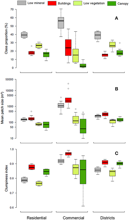
Figure 3. Land cover structure at 1 m spatial resolution. Each boxplot shows the distribution of a landscape metric value (y-axis) for residential (n = 10) and commercial zones (n = 10) as well as urban districts (n = 8) (x-axis). Each subfigure corresponds to a landscape metric: (A) class proportion; (B) mean patch size; (C) clumpiness index. Note that for mean patch size, the y-axis is on a logarithmic scale.

Effect of Map Aggregation on Representation of Land Cover Structure

On maps of residential and commercial zones as well as urban districts, the proportion of impervious surfaces (low mineral and buildings) generally increased, while the proportion of greenspaces (low vegetation and canopy) generally decreased with spatial aggregation (Figure 4). These effects were generally accentuated with increasingly coarse spatial resolution, but the magnitude varied between the three types of landscapes. On average, the proportion of impervious surfaces in residential zones increased by about 10%, while the proportion of greenspaces decreased by about −15% throughout the entire gradient of spatial resolution. In comparison, in commercial zones, the increase in proportion of impervious surfaces was less pronounced (+6% for low mineral and about zero for buildings), while the decrease in proportion of greenspaces was more pronounced (−27% for low vegetation and −46% for canopy). At the district level, the increase in proportion of impervious surfaces was intermediate to that of residential and commercial zones (+8% for low mineral and +4% for buildings), while the decrease in proportion of greenspaces was less pronounced than that of residential and commercial zones (−13% for low vegetation and −4% for canopy). In addition to these average values, the magnitude of the effect varied substantially within each type of landscape. For example, the variation in canopy proportion in commercial zones ranged from a +9% increase to a −100% decrease at 15 m, depending on which commercial zone was analyzed.

FIGURE 4

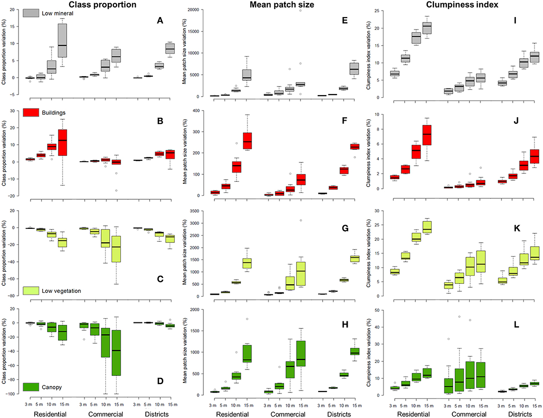
Figure 4. Variation of land cover structure at spatial resolutions of 3, 5, 10, and 15 m compared to land cover structure at a spatial resolution of 1 m. Each boxplot shows the distribution of a landscape metric variation (y-axis), each boxplot quartet shows variation at 3, 5, 10, and 15 m, and the three boxplot quartets in each subfigure correspond to residential zones (n = 10), commercial zones (n = 10) and urban districts (n = 8) (x-axis). Each column of subfigures corresponds to a landscape metric, while each row corresponds to a land cover class: (A) class proportion variation for low mineral; (B) class proportion variation for buildings; (C) class proportion variation for low vegetation; (D) class proportion variation for canopy; (E) mean patch size variation for low mineral; (F) mean patch size variation for buildings; (G) mean patch size variation for low vegetation; (H) mean patch size variation for canopy; (I) clumpiness index variation for low mineral; (J) clumpiness index variation for buildings; (K) clumpiness index variation for low vegetation; (L) clumpiness index variation for canopy. Note that the scale of y-axes differs between subfigures.

Regarding LC configuration, mean patch size and clumpiness index increased for each LC class and each landscape with map aggregation (Figure 4). Increase in mean patch size was generally more pronounced for low mineral, followed by low vegetation, canopy and then buildings (Y axes vary in scale). Regarding clumpiness, all LC classes tended to converge up to a high level of clumpiness at 15 m. Total percentage of changes was higher in residential (41% on average at 15 m) than commercial zones (14%), and intermediate in urban districts (29%) (Table 1). Visual analysis showed that changes occurred along the edge of large patches (stair-step effect), while small patches disappeared to the benefit of the dominant class surrounding them (Supplementary Figures A2.3, A2.6). The very large increase in mean patch size at 15 m in many landscapes could be related to the loss of almost all the very small LC patches with aggregation. In residential zones, low mineral gains occurred mainly at the expense of low vegetation, and mostly around roads. Small buildings and canopy patches disappeared from the map, while larger buildings and canopy patches coalesced into more clumped patches. In commercial zones, changes at the interface between low mineral and building patches resulted in gains and losses that mostly offset each other, while small low vegetation and canopy patches disappeared massively, mainly to the benefit of low mineral patches.

TABLE 1

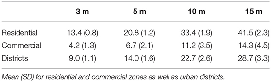
Table 1. Total percentage of cells that have changed LC class at spatial resolutions of 3, 5, 10, and 15 m compared to LC class at a spatial resolution of 1 m.

Quantity of Ecosystem Services Estimated at 1 m Spatial Resolution

Carbon storage (0.25 kgC/m²), cooling (1.19 units/m²) and pollination (0.05 units/m²) potential supply at 1 m resolution were on average lower in commercial than in residential zones and urban districts (Figure 5). Cooling flow (0.11 units/m²) was also lower in commercial zones, while null pollination flow was associated with the absence of gardens in these areas, and thus of demand. Comparing residential zones and urban districts, carbon storage (1.28 vs. 1.50 kgC/m²), cooling (2.91 vs. 3.24 units/m²) and pollination (0.09 vs. 0.11 units/m²) potential supply were on average similar, but pollination (1.52^*10⁻³ vs. 0.72^*10⁻³ units/m²) demand as well as cooling (0.5 vs. 0.35 units/m²) and pollination (0.15^*10–3 vs. 0.08^*10⁻³ units/m²) flow were on average higher in residential zones.

FIGURE 5

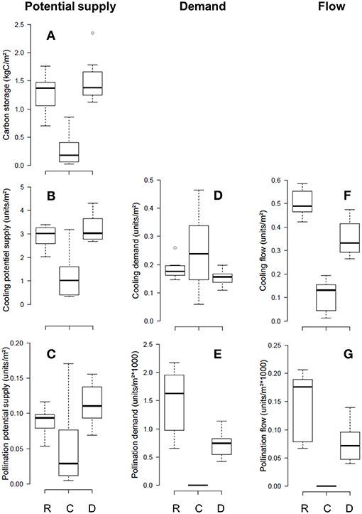
Figure 5. Ecosystem services quantity at 1 m spatial resolution. Each boxplot shows the distribution of ecosystem services quantity (y-axis) for residential (R; n = 10) and commercial zones (W; n = 10) as well as urban districts (D; n = 8) (x-axis). Each subfigure corresponds to an ecosystem service component: (A) carbon storage potential supply; (B) cooling potential supply; (C) pollination potential supply; (D) cooling demand; (E) pollination demand; (F) cooling flow; (G) pollination flow. Note that the scale of y-axes differs between subfigures.

Effect of Land Cover Resolution on Quantity of Ecosystem Services Estimated

For the three ecosystem services (ES) and each group of landscapes, ES potential supply and flow generally decreased with increasingly coarse LC data resolution (Figure 6). Carbon storage decreased in most landscapes (except the few where canopy cover increased with spatial aggregation; not shown). The effect of LC resolution on carbon storage was more variable and on average more pronounced in commercial (−38% at 15 m) than in residential zones (−13%) and urban districts (−4%).

FIGURE 6

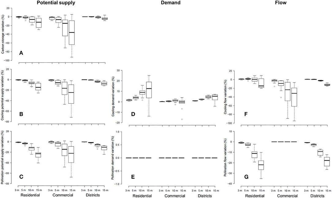
Figure 6. Variation of ecosystem services quantity at spatial resolutions of 3, 5, 10, and 15 m compared to ecosystem services quantity at a spatial resolution of 1 m. Each boxplot shows the distribution of ecosystem services quantity variation (y-axis), each boxplot quartet shows variation at 3, 5, 10, and 15 m, and the three boxplot quartets in each subfigure correspond to residential zones (n = 10), commercial zones (n = 10), and urban districts (n = 8) (x-axis). Each subfigure corresponds to an ecosystem service component: (A) carbon storage potential supply variation; (B) cooling potential supply variation; (C) pollination potential supply variation; (D) cooling demand variation; (E) pollination demand variation; (F) cooling flow variation; (G) pollination flow variation. Pollination demand variation is null because the spatial resolution of the pollination demand map was kept constant at 1 m for each model run. Pollination flow variation in commercial zones is null because there was no pollination demand and thus no pollination flow in these zones. Note that the scale of y-axes differs between subfigures.

Following a pattern similar to that of carbon storage, the quantity of cooling flow decreased in most landscapes, with the effect of LC resolution again being more variable and on average more pronounced in commercial zones (−41% at 15 m) than in urban districts (−12%) and residential zones (−9%) (Figure 6). Variability in the effect of LC resolution on cooling flow was very low for districts, but intermediate for residential zones, where cooling flow increased in some zones. This increase likely resulted from an increase in cooling demand that largely compensated for the decrease in potential supply in these zones. However, variation in the quantity of cooling flow was not simply the sum of variation in the quantity of potential supply and demand, but also depended on changes in their spatial configuration. Indeed, cooling flow generally decreased more than would be expected based on the variation in potential supply and demand, indicating that the decrease in potential supply was more pronounced near buildings than, on average, in the entire landscape (Figure 7). In other words, this indicates that the decrease in greenspace cover was more pronounced in a 60 m radius around buildings than in the landscape as a whole.

FIGURE 7

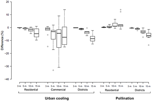
Figure 7. Difference between (1) variation of ecosystem services flow at spatial resolutions of 3, 5, 10, and 15 m compared to ecosystem services flow at a spatial resolution of 1 m, and (2) the sum of variation of ecosystem service potential supply and demand at spatial resolutions of 3, 5, 10, and 15 m compared to ecosystem service potential supply and demand at a spatial resolution of 1 m. Each boxplot shows the distribution of the difference (y-axis), each boxplot quartet shows variation at 3, 5, 10, and 15 m, and the five boxplot quartets correspond to residential zones (n = 10), commercial zones (n = 10), and urban districts (n = 8) for cooling and pollination (x-axis). Note that two outlier data points are excluded from the figure to optimize presentation.

Pollination flow decreased in every residential zone and urban district (Figure 6). This decrease was slightly more variable and more pronounced in residential zones than in urban districts (−22 vs. −19% at 15 m). While demand did not vary in either of these types of landscapes, the decrease in pollination flow was not equal to that in pollination potential supply, again indicating that the variation in potential supply was not uniform across the landscape. In residential zones, decrease in flow was generally less pronounced than that in potential supply, indicating that the latter was less pronounced around gardens than elsewhere (Figure 7). Conversely, in districts, decrease in flow was generally more pronounced than that in potential supply, indicating that the latter was more pronounced around gardens than elsewhere.

Discussion

Effect of Spatial Resolution on Maps of Urban Land Cover and Ecosystem Services

Our results suggest that using land cover (LC) data with a spatial resolution coarser than 1 m can be expected to lead to underestimating greenspace cover and ecosystem services (ES) potential supply in urban areas. However, a decrease in ES potential supply with LC aggregation did not necessarily result in a proportional reduction in ES flow. For example, in some residential zones, a higher demand for urban cooling counterbalanced a lower potential supply at a coarser resolution, leading to a higher cooling flow. In addition, variation in ES flow also depended on changes in the spatial configuration of ES potential supply relative to demand. Decrease in cooling and pollination flow depended on changes in greenspace cover specifically around buildings and gardens, which were usually different from changes calculated for entire landscapes. These differences between potential supply, demand, and flow variation demonstrate the importance of considering the specific location of LC changes when assessing the effect of LC resolution on mapping spatial flows of ES from provisioning to benefiting areas.

All other factors being equal, the effect of LC resolution should thus be easier to estimate for global-flow ES that depend only on changes in potential supply, than for local-flow ES that also depend on the specific location of changes in potential supply relative to demand. These two scales of spatial flow represent extremes on a continuum from local to global scale, and the sensitivity of regional-flow ES (i.e., flood control or water provisioning) will probably be intermediate. For example, the specific location (e.g., meter-accurate) of changes in LC may not be significant for modeling water provision in a watershed, but it could be necessary to distinguish between changes that occur upstream and downstream from water intake. Changes in LC configuration would also need to be assessed to estimate the effect of LC resolution on mapping of potential supply using a spatially explicit model. For instance, potential supply often depends on the location of a provisioning area in the landscape (e.g., riparian vs. non-riparian) or on its position relative to other LC classes (e.g., connecting areas) (Andersson et al., 2015;Verhagen et al., 2016).

The trend toward a decrease in low vegetation and canopy cover to the benefit of low mineral and building cover observed with aggregation in this study is coherent with findings in the literature (e.g., Qian et al., 2015a,b; Zhou et al., 2018). As cell size increases, classes with a higher initial proportion and clumpiness tend to increase in proportion, at the expanse of rarer and more dispersed classes (Turner et al., 1989). Likewise, the increase in clumpiness and mean patch size observed with aggregation for every class and landscape was expected, as it is the consequence of small patches coalescing into larger ones (Moody and Woodcock, 1995). These changes in LC configuration probably increased the average distance between buildings and greenspace cells, the former falling outside of the flow area, which could explains the accentuated decrease in cooling flow. Such loss of information on fine-scale spatial heterogeneity may thus be particularly crucial for local-flow ES that depend on the proximity between provisioning and benefiting areas.

The underestimation of greenspace cover with increasingly coarse spatial resolution must, however, be viewed as a tendency rather than a definitive pattern, as the effect of LC aggregation varied between types of landscapes. In particular, the decrease in greenspace cover and ES potential supply was less pronounced in urban districts than in residential and commercial zones. This indicates that variation in greenspace cover was positive (or less negative) in the “other” land use (LU) types composing the districts, which can be related to the presence of large greenspaces like parks. More generally, the differences between districts and residential and commercial zones underscore the importance of considering intra-urban variability in LC structure when estimating the effect of LC resolution on mapping of urban ES. Analysis at the level of local zones homogeneous in terms of LU allowed us to control some of this variability and highlight meaningful differences between residential and commercial LU types. For example, decrease in greenspace cover was on average more pronounced in commercial than in residential zones, because the initial proportion of greenspaces was lower and there were fewer gains possible for low vegetation and canopy patches against the large impervious surfaces patches surrounding them. A better understanding of these local characteristics can support a more accurate estimate of the effect of LC aggregation within the urban area. For example, knowing that low vegetation losses with aggregation in residential areas mostly occur in front yards can be useful when mapping an ES for which location relative to the road network is important, like surface runoff attenuation (Alberti et al., 2007).

The variable effect of LC aggregation found for urban districts and residential and commercial zones was also evident within each type of landscape. For residential and commercial zones, one factor that partially explains this variability is that LU is only an imperfect approximation of LC structure (Vanderhaegen and Canters, 2017). This was particularly apparent for commercial zones, where the initial LC structure at 1 m was highly variable. However, even for residential zones where the initial LC structure was similar between zones, large differences in LC response were observed, indicating that even a small change in initial LC structure could influence the effect of aggregation. This sensitivity can be expected to be particularly high when cell size is near the grain of the landscape (Woodcock and Strahler, 1987), as was the case in fine-grained residential zones, where a high number of changes was observed on a cell-by-cell basis. A way to reduce the variability found for residential and commercial zones would be to refine the definition of LU types by, for example, distinguishing several residential densities (e.g., low, medium, and high density). However, some levels of variability will always persist because any LU classification system remains an abstraction of an urban continuum (Vanderhaegen and Canters, 2017). Consequently, rather than using LU as a proxy, it may be possible to characterize the LC structure of a landscape unit directly with a set of landscape metrics, and then assess the relationship between this structure and the effect of spatial resolution using statistical analysis. This approach has proved effective for correcting errors in class area estimates at coarser resolution in forested landscapes (Moody and Woodcock, 1995). However, the statistical model developed for a given landscape may not apply in another landscape, as many LC attributes are interactive (Moody and Woodcock, 1996; Francis and Klopatek, 2000). A combination of the empirical LU based approach tested in this study, establishing the general landscape structure, with the statistical approach mentioned above, specifying landscape attributes with a subset of significant metrics, would merit further investigation.

The generally lower variability observed for urban districts compared to residential and commercial zones was surprising, since the former were composed of a heterogeneous mix of different LU types and were not selected for their similarity. The larger expanse of urban districts, compared to the smaller sized residential and commercial zones, probably buffered the results by moderating the influence of “extreme” local effects. As well, our focus only on the urban part of each district, rather than its entirety, may have fostered LC similarity between districts and contributed to convergence of results. Using a quantitative method based on surface imperviousness to delineate the urban area may thus provide a way to control the variability in LC structure and help estimate the effect of spatial resolution on LC representation and ES mapping. However, the low variability observed for urban districts may also be specific to our study area. It would be interesting to compare these results with those of other cities, using the same definition of urban area, to assess their robustness. In particular, the effect of LC resolution in cities exhibiting alternative forms of development (e.g., level of density), history (e.g., former LU), and natural setting (e.g., climate) should be assessed. Our results should be representative of low-density suburban areas, as the city of Laval is a typical example of such suburbs (Dupras et al., 2016; Nazarnia et al., 2016), but caution should be taken when applying our quantitative results to more compact cities, such as those in Europe or Asia (Welch, 1982). For instance, European cities have been shown to develop differently than North American ones, mainly due to stronger planning legislation and availability of public transportation (Nazarnia et al., 2016).

Before considering whether the empirical results presented in this study are applicable elsewhere, it is also essential to be aware of the methodological factors that influence the effect of LC aggregation. First, the LC classification system used defines the initial LC map structure and therefore its response to aggregation (Ju et al., 2005). For example, disaggregating the “low mineral” class into asphalt, concrete and other types of material would result in less dominant classes that would probably not increase with aggregation as much as “low mineral” did. Second, our results cannot be readily extrapolated beyond the range of spatial resolution considered (1–15 m), as landscape structure is scale dependent (Wu, 2004). Third, we documented the effect of LC aggregation following a majority rule, which is only one method among many others (e.g., Raj et al., 2013). We chose the majority method because it is commonly used in ecology and remote sensing (Wu, 2004) and for its similarity to producing LC maps directly from aerial or satellite images of variable resolutions (Benson and MacKenzie, 1995). However, the outcomes of aggregating an existing LC map and producing several LC maps from images of different resolutions are not identical (Turner et al., 2000; Schulp and Alkemade, 2011). In addition, between two distinct LC products representing a given landscape, there will always be differences other than those caused by spatial resolution, stemming, for example, from temporal differences or classification errors. These additional differences should also be considered when assessing the effect of LC data input on ES mapping.

Implications for Mapping Urban Ecosystem Services

The continuous growth of urban areas and human populations poses a great challenge for ensuring human well-being in cities (Haase et al., 2014). Urbanization processes, either sprawl or densification, generally result in the reduction of land areas covered by vegetation within the urban matrix. Planning for urban greenspaces may be a solution that would contribute to the development of sustainable cities, since these spaces promote physical activity, psychological well-being, and the general public health of urban dwellers through the delivery of essential ES benefits (Bolund and Hunhammar, 1999; Tzoulas et al., 2007; Niemalä et al., 2010; Irvine et al., 2013). However, to make informed management choices, planners and decision makers need to rely on data that are consistent with the level of accuracy required. Our results showed that aggregating LC data from 1 to 15 m can result in substantially underestimating greenspace cover and, as a direct consequence, ES quantity. Considering the difficulty of making accurate estimates, and subsequently correcting for this effect, our study reaffirms the importance of choosing data of appropriate resolution for mapping urban ES (see also Grafius et al., 2016). Although the aim of this study was not to identify a single optimal spatial resolution for mapping urban ES, our results suggest the use of LC data with a spatial resolution of 5 m or higher. Such high resolution LC data is needed to detect the small greenspaces scattered throughout the urban matrix, which can represent a significant proportion of total urban vegetation cover (Qian et al., 2015a,b; Zhou et al., 2018) and thus of ES potential supply.

Using high resolution LC data is recommended to accurately map the ES produced by greenspaces, particularly for local-flow ES like urban cooling, which must be supplied near the beneficiaries, inside the urban matrix. Indeed, those small greenspaces scattered throughout the urban matrix will often be located closer to ES demand and thus provide the actual ES flows. An accurate representation of the spatial configuration of ES potential supply relative to ES demand is also essential to adequately map these local flows of ES. Failing to capture the fine-scale spatial relation between ES provisioning and benefiting areas could lead to erroneous greenspace management decisions, such as displacing management interventions (e.g., conservation, restoration, creation, etc.) toward locations that are suboptimal in terms of ES benefits delivery. For instance, when the ES being evaluated is supplied only by large greenspaces (e.g., recreation in urban parks), the consequences of using coarser LC maps may not be significant but finer resolution maps may be necessary for making decisions on specific management options, such as where trees should be planted along city streets in order to obtain maximal benefits (e.g., McPherson et al., 2011). Benefits for a tree planting program in the city of Los Angeles have been estimated $1.33 billion on average over the next 35 years (McPherson et al., 2011), indicating that management decisions on where to locate trees may indeed have significant economic consequences. Estimating where the most important ES flows would be following plantation, and avoiding location errors, could increase the effectiveness of such management decisions.

Our results also provide a number of meaningful insights into the quantification of ES that should be considered in most analyses and applications. First of all, in addition to the total quantity of ES in an area, it could be important to consider the effect of LC resolution on other aspects of ES maps, like the location of ES hotspots, bundles or mismatches (Bennett et al., 2009; Geijzendorffer et al., 2015; Schroter and Remme, 2016). For example, Cimon-Morin and Poulin (2018) used ES supply, demand and flows to assemble a conservation network for protecting ES delivered by urban wetlands. It would therefore be interesting to assess whether changing LC resolution modifies site priority status and network costs (efficiency), or if site ranking remains similar despite the overall change in ES supply, demand and flow. Our results could also help reconcile urban management challenges with environmental justice issues. Indeed, many studies on urban greenspace have revealed that the distribution of such infrastructures often predominantly benefits specific groups, such as more affluent, predominantly white communities in American cities (Wolch et al., 2014). A better quantification of ES flows, and thus, of accessibility to ES benefits for a diversity of groups and communities, may foster effective strategies to lower such inequalities by directly targeting areas that reap few greenspace benefits. It should also be helpful for determining the greenspace surface area required to avoid counteractive effects of greening strategies, such as increased housing costs and property values, gentrification and displacement of the residents who were the intended beneficiaries (Dooling, 2009; Wolch et al., 2014).

Data Availability

The datasets generated for this study are available on request to the corresponding author.

Author Contributions

J-FR organized the database, performed the analyses, and wrote the first draft of the manuscript. All authors contributed to the conception and design of the study, manuscript revision, read, and approved the submitted version.

Funding

J-FR was supported by study grants from the Natural Sciences and Engineering Research Council of Canada (NSERC), the Fonds de recherche du Québec—Nature et technologies (FRQNT), the Quebec Center for Biodiversity Science (QCBS) and the Institut Hydro-Québec en Environnement, Développement et Société (Institut EDS). MP and SP received funding form the NSERC (discovery grants RGPIN-2014-05663 and RGPIN-2014-05367, respectively). DA benefited from a research period at Université Laval as invited Professor for the 2017-18 academic year.

Conflict of Interest Statement

The authors declare that the research was conducted in the absence of any commercial or financial relationships that could be construed as a potential conflict of interest.

Acknowledgments

The authors would like to thank S. Uhde for sharing ideas and suggestions during a preliminary phase of the study, and M. Darveau and R. Fournier for their constructive comments on an early draft of this article. Special thanks to K. Grislis for stylistic revision of the manuscript. This research was conducted as part of a master project. The results presented in this article are also included in the master thesis of J-FR. This thesis will be accessible online by December 17, 2019. Until then, only the abstract is available online: http://hdl.handle.net/20.500.11794/33306.

Supplementary Material

The Supplementary Material for this article can be found online at: https://www.frontiersin.org/articles/10.3389/fenvs.2019.00093/full#supplementary-material

References

Alberti, M., Booth, D., Hill, K., Coburn, B., Avolio, C., Coe, S., et al. (2007). The impact of urban patterns on aquatic ecosystems: an empirical analysis in puget lowland sub-basins. Landsc. Urban Plan. 80, 345–361. doi: 10.1016/j.landurbplan.2006.08.001