 Andreas F. Prein
 Melissa S. Bukovsky
 James M. Done
94% of researchers rate our articles as excellent or good
Learn more about the work of our research integrity team to safeguard the quality of each article we publish.
Find out more
ORIGINAL RESEARCH article
Front. Environ. Sci. , 10 April 2019
Sec. Atmospheric Science
Volume 7 - 2019 | https://doi.org/10.3389/fenvs.2019.00036
This article is part of the Research Topic Modelling, Simulating and Forecasting Regional Climate and Weather View all 12 articles
Regional climate models (RCMs) are able to simulate small-scale processes that are missing in their coarser resolution driving data and thereby provide valuable climate information for climate impact assessments. Less attention has been paid to the ability of RCMs to capture large-scale weather types (WTs). An inaccurate representation of WTs can result in biases and uncertainties in current and future climate simulations that cannot be easily detected by standard model evaluation metrics. Here we define 12 hydrologically important WTs in the contiguous United States (CONUS). We test if RCMs from the North American CORDEX (NA-CORDEX) and the Weather Research and Forecasting (WRF) model large physics ensembles (WRF36) can capture those WTs in the current climate and how they simulate changes in the future. Our results show that the NA-CORDEX RCMs are able to simulate WTs more accurately than members of the WRF36 ensemble. The much larger WRF36 domain in combination with not constraining large-scale conditions by spectral nudging results in lower WT skill. The selection of the driving global climate model (GCM) has a large effect on the skill of NA-CORDEX simulations but a smaller impact on the WRF36 runs. The formulation of the RCM is of minor importance except for capturing the variability within WTs. Changing the model physics or increasing the RCM horizontal grid spacing has little effect. These results highlight the importance of selecting GCMs with accurate synoptic-scale variability for downscaling and to find a balance between large domains that can result in biased WT representations and small domains that inhibit the realistic development of mesoscale processes. At the end of the century, monsoonal flow conditions increase systematically by up to 30% and a WT that is a significant source of moisture for the Northern Plains during the growing seasons decreases systematically up to –30%.
Regional climate models (RCMs) are designed to dynamically downscale larger-scale climate data over a region of interest to capture regional-scale processes that are not present in the driving model (Giorgi, 1990; Denis et al., 2002; Rummukainen, 2010). Many studies address the added value of RCM downscaling, which are mainly found on local to regional-scales (Feser et al., 2011; Di Luca et al., 2012; Prein et al., 2016a) in regions with complex orography, areas with strong land-surface heterogeneities, and in atmospheric situations with strong spatial gradients that are often related to extreme events (Rummukainen, 2016). It is more unclear if RCMs can also add value to the large-scale patterns of their driving model by upscale growth of mesoscale processes. However, there are a few examples in the published literature such as improvements of rain shadow effects due to the better representation of orography (Leung et al., 2003), or downstream effects of mesoscale convective vortices in the US (Clark et al., 2010).
The evaluation of RCMs is typically performed on a seasonal basis using standard atmospheric variables such as near-surface temperature and precipitation (Christensen et al., 2007a; Mearns et al., 2012; Kotlarski et al., 2014; Prein et al., 2016a). While this can provide a broad assessment of model skill it typically does not allow in-depth insights to understand errors in specific modeled processes. This is partly due to combining local- and large-scale errors in the analysis. Addor et al. (2016); for example, showing that a general wet bias of RCM simulated wintertime precipitation in the European Alps can be related to an overestimation of westerly flow regimes.
Weather typing (WTing) was initially developed for weather forecasting (e.g., van Bebber, 1891). In more recent decades, studies used WTing to downscale large scale circulation patterns to local scales (Goodess and Palutikof, 1998; Wood et al., 2016), evaluate global climate model performance (Radić and Clarke, 2011; Gibson et al., 2016), to understand changes in observed climate trends (Paredes et al., 2006; Prein et al., 2016b), and to assess future climate projections in terms of changing large-scale dynamics (Santos et al., 2016).
Here we use hydrologically important WTs to investigate the ability of two ensembles of RCM simulations to capture large-scale atmospheric patterns over the contiguous United States (CONUS). The two ensembles are the North American contributions to the Coordinated Regional Climate Downscaling Experiment (NA-CORDEX; Mearns et al., 2017) and the National Center for Atmospheric Research's (NCAR's) 36 km grid spacing Weather Research and Forecasting (WRF) model physics ensemble (WRF36; Bruyère et al., 2017).
Using WT for model evaluation has two main advantages: (1) We focus solely on the RCM's ability to represent synoptic-scale patterns, which allows separating model biases in large-scale dynamics and thermodynamics and mesoscale components, and (2) RCM errors are typically process-dependent and, therefore, RCMs have different bias characteristics in different seasons (e.g., Mearns et al., 2012; Kotlarski et al., 2014). However, seasons consist of a mix of various weather regimes and atmospheric processes. Seasonally based analyses can be viewed as a zero order approximation of a weather regime-dependent analysis. Performing model evaluation based on WTs helps to separate atmospheric processes more accurately and allows insights into regime-specific model performance.
The goal of this study is 2-fold. (1) We aim to understand which components of an RCM setup affects its capability to simulate WTs over the CONUS. The analyzed components are the driving GCM, the formulation of the RCM, sensitivities to RCM model physics, RCM horizontal grid spacing, and RCM domain size. The goal is to provide guidance for future RCM downscaling studies. (2) We want to understand if there are systematic changes in future climate WT frequencies. Enhancing our understanding of climate impacts on large-scale dynamics is important since almost all confidence that we have regarding future climate projections is based on thermodynamic processes (Shepherd, 2014).
The paper is structured as follows. Section 2 summarizes the used RCM simulations and the WT method. Section 3 describes the main characteristics of the derived WTs, presents the results from the RCM evaluation, an assessment of the sources of performance variability, and WT changes in climate projections. Section 4, 5 summarize the findings and conclude the study.
We use RCM simulations from the NA-CORDEX and the WRF36 ensemble datasets. RCMs participating in the NA-CORDEX ensemble downscale ERA-Interim (Dee et al., 2011) and global climate models (GCMs) from the CMIP5 archive (Taylor et al., 2012) over a common region that covers most of North America (see blue domains in Figure 1). The domain sizes vary slightly between the participating RCMs. The ERA-Interim driven simulations cover a common period from 1989 to 2010, while the GCM driven runs at least cover 1951–2099. Most RCMs have a horizontal grid spacing of 0.44°/50 km and the WRF simulations are also available at 0.22°/25 km grid spacing. We only use a subset of the full NA-CORDEX simulations for which the necessary WTing variables are available. We use simulations performed with WRF (Skamarock and Klemp, 2008), the Danish Meteorological Institute's HIRHAM5 model (Christensen et al., 2007b), the UK Met Office's HadRM3P model (Jones et al., 1995; Buonomo et al., 2007), and the Canadian Regional Climate Model version 5 (Caya and Laprise, 1999; Zadra et al., 2008; Martynov et al., 2013; Šeparović et al., 2013, CRCM5; ). These RCMs downscale five different GCMs with historical and RCP4.5 and RCP8.5 concentration scenarios (Van Vuuren et al., 2011). The WRF simulations used spectral nudging to constrain synoptic scales according to those of the driving model in the domain interior. This is important since with this setting WTs should not be able to deviate significantly from those in the driving model. No spectral nudging was used in the other RCM simulations. A list of all NA-CORDEX simulations is shown in Table 1 and more details on the model setup can be found in Table 2 and online under https://na-cordex.org/rcm-characteristics.
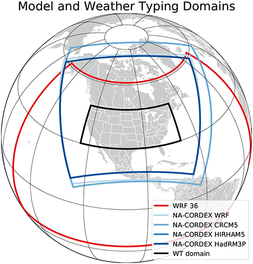
Figure 1. Model (colors) and weather typing domains (black rectangle). The WRF36 domain is shown in red and the NA-CORDEX domains are shown in blue.
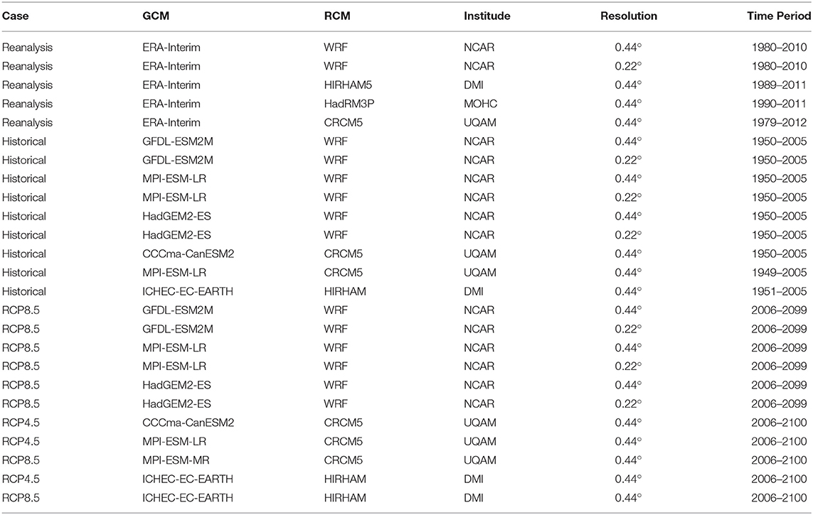
Table 1. NA-CORDEX simulations used in this manuscript.
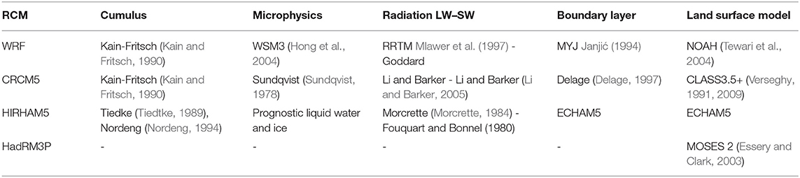
Table 2. Major characteristics of the NA-CORDEX RCMs.
NCAR's WRF36 RCM ensemble (Bruyère et al., 2017) is targeted toward understanding uncertainties from model physics and consists of 24 members of WRF simulations that downscale ERA-Interim within the period from 1990 to 2000 with 36 km horizontal grid spacing. The model domain is substantially larger than the domains used in the NA-CORDEX simulations and covers most of the North and Central Atlantic, the east Pacific, most of North America, central America, and northern South America (Figure 1). The motivation for this large domain was to decouple the RCM simulations from their lateral boundary conditions to improve the representation of mesoscale processes. In theory, such improvements should be possible due to the better representation of mesoscale forcing such as orography in addition to atmospheric processes, e.g., tropical cyclones, and teleconnections in the higher resolution RCM (e.g., Erfanian and Wang, 2018).
Table 3 shows the 24 ensemble members that downscale ERA-Interim by systematically varying four physics parameterizations: (1) cumulus [KF: (Kain and Fritsch, 1990); NSAS: (Han and Pan, 2011); and Tiedtke: (Tiedtke, 1989)], (2) radiation [CAM: (Collins et al., 2006) and RRTMG: (Mlawer et al., 1997)], (3) microphysics [WSM6: (Han and Lim, 2006) and Thompson: (Thompson et al., 2004)], and (4) planetary boundary layer [MYJ: (Janjić, 1994) and YSU: (Hong et al., 2006)]. In this study, we abbreviate members of this ensemble by four characters. The first character denotes the radiation scheme, the second the cumulus scheme, the third the microphysics, and the fourth the planetary boundary layer parameterization. For example, the RNTY member uses the RRTMG radiation, NSAS cumulus, Thompson microphysics, and YSU boundary layer scheme. The selected physics are well tested and widely used.
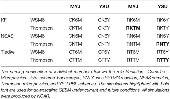
Table 3. The physics combination of the WRF36 ensemble that used ERA-Interim between 1990–2000 as driving data.
After evaluating the 24-member ensemble, three members were selected to perform additional current and future climate downscaling experiments. These three members are the RKTM, RNTY, and RTTY simulations. They downscale a free running GCM simulation performed by the Community Earth System Model (CESM; Hurrell et al., 2013), which is part of the CMIP5 experiments (Taylor et al., 2012). CESM is one of the best performing models in the CMIP5 ensemble based on its ability to simulate global temperature and precipitation patterns (Knutti et al., 2013). This simulation uses the business as usual RCP8.5 emission scenario for future climate projections (Van Vuuren et al., 2011). To reduce biases in CESM's lateral boundary conditions, a bias correction method described in Bruyère et al. (2014, 2015) was applied prior to the downscaling. This method only bias corrected the mean base state, leaving the synoptic variability, interannual variability, and any climate trend unchanged. The CESM driven WRF36 simulations cover the periods 1990 to 2000, 2020 to 2030, 2030 to 2040, 2050 to 2060, and 2080 to 2090. Additional information about the WRF36 simulations can be found in Bruyère et al. (2017).
The most notable differences between the WRF36 simulations and WRF experiments from the NA-CORDEX are the computational domain size and the use of spectral nudging in the latter (von Storch et al., 2000). The physics in the RK6M simulation are very similar to those used in NA-CORDEX except for the microphysics, which are more simplistic in the latter. The NOAH land surface model (Tewari et al., 2004) is used in both ensembles.
The variables used for the WTing are derived from daily ERA-Interim data at 12 UTC (Dee et al., 2011). ERA-Interim is a third generation reanalysis, which has very high skill in representing atmospheric processes compared to other reanalysis products (e.g., Decker et al., 2012; Lin et al., 2014).
For precipitation analyses we use the Parameter-elevation Relationships on Independent Slopes Model (PRISM) daily gridded precipitation data within the period from 1980 to 2014 (Daly et al., 1994). PRISM is based on ~13 000 surface stations for precipitation including USDA NRCS Snow Telemetry (SNOTEL) and snowcourses data (http://www.wcc.nrcs.usda.gov/snow/) to capture mountain snow pack.
The performed WTing is similar to the algorithm used in Prein et al. (2016b) and (Prein, under review). It is a combination of two clustering methods: a hierarchical cluster analysis and a k-means cluster analysis that uses the outcome of the hierarchical clustering as the starting partition (Romesburg, 2004). This approach showed very high skill in classifying WTs in a WT method comparison study over the European Alps (Schiemann and Frei, 2010) and was successfully applied in many weather typing analyses (e.g., García-Valero et al., 2012; Lorente-Plazas et al., 2015). Daily ERA-Interim data from 1979–2014 is used over the CONUS (see black rectangle in Figure 1) to define representative WTs capturing the main variability of precipitation in this region. We use a moving average Gaussian high-pass filter of 31-day length to remove variability longer than those of typical synoptic-scale patterns, e.g., the seasonal cycle. This does not affect the spatial patterns of the daily input variables. Afterward, we normalize each input variable to generate fields with equal weights as input for the WT analysis.
We used two metrics to test the skill of the derived WTs. (1) We aim to minimize the intracluster to intercluster variance (Straus and Molteni, 2004) of the daily CONUS wide precipitation patterns in each WT. The goal is to cluster days with similar precipitation patterns within one WT and to obtain WTs having different precipitation patterns when compared to each other. (2) In addition, we want to maximize the average absolute precipitation anomalies of each WT centroid. The WT centroid is the average over each cluster element, e.g., average precipitation anomaly of each day within a WT. This metric ensures that WTs are as different as possible from the climatological average precipitation in the CONUS.
Figure 2 summarizes the results for the WT skill analysis, which is dependent on the number of used WTs and the input variables. We tested a variety of input variable combinations. Horizontal wind speed at 500 hPa (UV500), sea level pressure (SLP), and precipitable water (PW) are available on a daily basis for most RCM simulations. These are important variables for many dynamic and thermodynamic processes related to precipitation (Doswell III et al., 1996; Lin et al., 2001). Using 12 WTs with these variables lead to a skillful representation of hydrologically important weather patterns in the CONUS. Twelve WTs seem to be sufficient since adding more WTs only leads to marginal improvements in clustering skill (Figure 2). These results are similar to work by Prein et al. (2016b) except that we used 500 hPa instead of 700 hPa wind speed since the latter was not available for many NA-CORDEX simulations.
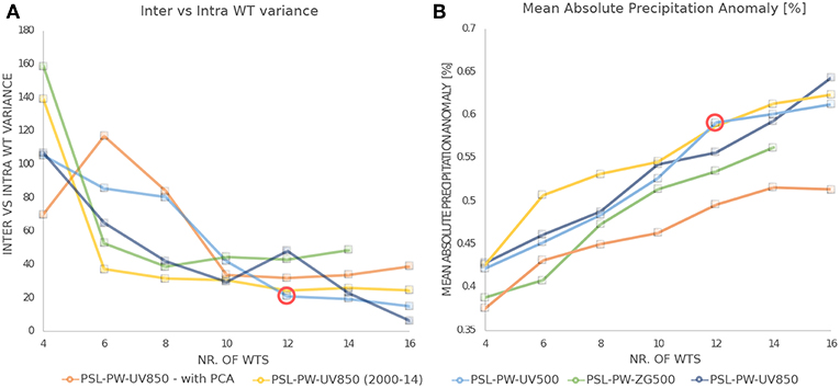
Figure 2. Assessment of the clustering strength of WTs. (A) Inter- vs. intra-cluster variance and (B) absolute precipitation anomalies averaged over all WTs. Different colors show different WT settings. The tested input variables are sea level pressure (SLP), precipitable water (PW), wind speed at 850 hPa/500 hPa (UV850/UV500), and 500 hPa geopotential height (ZG500). We also test the impacts of using a principal component analysis (PCA) before the WT clustering and the length of the clustering period, which is 1979–2014 unless otherwise denoted. The red circle shows the final WT setup using 12 WTs and SLP, PW, and UV500 as input variables.
The WTing on ERA-Interim data results in a WT time series that assigns a WT to each day within the period of 1979–2014. This time series allows us to calculate WT centroids (Figure 3), which are used to assign WTs to each day in the RCM output.
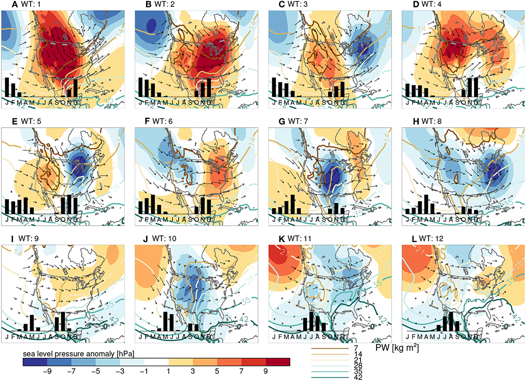
Figure 3. Centroids of the 12 ERA-Interim based WTs (A–L) for the period 1979–2014. Filled contours show sea level pressure anomalies, green contour lines show precipitable water (PW), and arrows show 500 hPa wind direction and speed. A histogram of the relative frequency of each WT is shown in the bottom left and the domain used for the WTing is shown in the gray dashed box.
To assign WTs to the RCM output we first conservatively remap daily simulated SLP, UV500, and PW fields to the ERA-Interim grid. Then we apply a 31-day moving average Gaussian high-pass filter to the remapped data and normalize the variables similarly to what we have done to the ERA-Interim data. Thereafter, we calculate the average Euclidean distances of each input variable for each day in the RCM simulations to the 12 ERA-Interim WT centroids that are described above. Each day is assigned to the centroid with the minimum average Euclidean distance.
The resulting WTs show distinct differences in SLP anomalies, 500 hPa wind speed and direction, and PW values within the CONUS (Figure 3). We sorted the WTs from predominantly winter patterns (WT1–4) to shoulder season WTs (WT5–10) and summer WTs (WT11 and WT12). The different flow regimes result in distinct precipitation anomaly patterns (Figure 4). WT1 is most frequent in December and January and it is characterized by a strong high-pressure anomaly with dry air advection from the northwest into the central US (Figure 3A). This results in anomalous dry conditions in most of the US (Figure 4A). In WT2 the high-pressure anomaly is shifted toward the Midwest favoring moisture transport to the west coast (Figure 3B), resulting in wetter than average conditions in this region (Figure 4B). WT3 has a January maximum and high/low-pressure anomalies in the western/eastern half of the CONUS (Figure 3C), which lead to predominantly dry conditions (Figure 4C). Very wet conditions in the eastern CONUS occur in WT4 (Figure 4D), which has an early winter peak. This is due to strong moist air advection from the Pacific and Gulf of Mexico into the continent (Figure 3D). Similar precipitation anomalies are caused by WT5 (Figure 4E) as a result of a strong low-pressure anomaly over the Great Lakes region. WT6, WT7, and WT8 occur predominantly in spring and are the main sources of precipitation in the US Southwest (Figures 4F–H). They are associated with low-pressure anomalies over the western half of the CONUS and moist air advection from the Pacific (Figures 3F–H). WT7 results in anomalously wet conditions in the upper Plains, the Midwest, and the Deep South due to its strong low-pressure anomaly in the central US. Weak flows and predominantly dry conditions are present during the spring WT9 except for parts of Texas and New Mexico (Figures 3I, 4I). Very wet conditions are present in the upper Plains during WT10 conditions due to a low-pressure anomaly and moisture advection into this region (Figures 3J, 4J). WT11 is a typical summer WT with high PW values in the eastern CONUS and wetter than average conditions in this area (Figures 3K, 4K). Monsoonal flow conditions are present in the late summer WT12 with high precipitation anomalies in Arizona and New Mexico (Figures 3L, 4L).
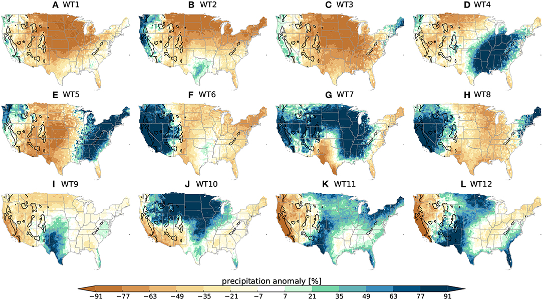
Figure 4. Precipitation anomalies for each WT (A–L) based on the PRISM daily gridded observational data between 1981 and 2014 (Daly et al., 1994).
The following analysis is based on data that cover the common evaluation period of 1990–2000. Due to this rather short period, the results might be affected by internal climate variability. Therefore, we focus our analysis on systematic differences between the two ensembles and their members rather than the performance of individual simulations.
There is a large spread in how well RCMs capture observed WT frequencies (Figure 5). The frequencies of WT5 and WT9 are well captured by most simulations whereas other WTs, such as WT4, show systematic low biases. It is important to mention that a high-frequency bias in one WT has to be counteracted in low biases in other WTs. Simulated WT frequency biases will result in precipitation biases since the WTs are associated with pronounced precipitation anomalies. For example, most simulations have a low-frequency bias for WT4 patterns, which results in cold season conditions that are too dry in the Deep South and Appalachian region, since WT4 is one of the main contributors of precipitation in those regions (see Figure 4D). Such a bias is frequently found in recent RCM simulations (Mearns et al., 2012).
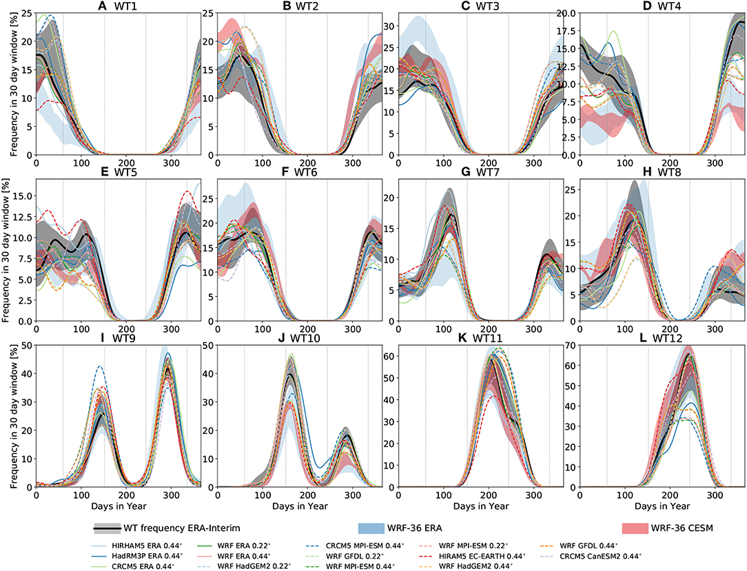
Figure 5. Annual cycle of WT frequencies smoothed by a Gaussian low-pass filter with 10-day standard deviation for each of the 12 WTs (A–L). The thick black line shows ERA-Interim WT frequencies for the period 1990–2000 and the gray contour shows the spread in all possible 11-year contiguous ERA-Interim periods within 1979–2014 as an estimate of climate variability. The blue contour shows the spread in the 24-member WRF36 ensemble that uses ERA-Interim as driving data. The red contour shows the spread within the 3-member CESM driven WRF36 hindcast simulations. Colored solid/dashed lines show WT frequencies in NA-CORDEX hindcast/historical simulations. The RCM results are based on the period 1990–2000. Vertical dashed lines show the end of February, May, August, and November respectively from left to right.
A more systematic analysis of WT frequency biases is shown in Figure 6. The most striking feature is that NA-CORDEX simulations better capture WT frequencies than WRF36 simulations. This is likely related to the much larger domain size and not applying spectral nudging in the WRF36 simulations which allows them to deviate from the large-scale conditions provided by the driving data.
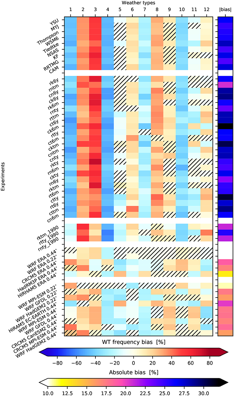
Figure 6. Heatmap showing average WT frequency biases (smaller is better) for simulations (rows) and WTs (columns), and the absolute bias averaged over all WT biases in the rightmost column (lower color bar). The top block shows biases for WRF36 ERA-Interim simulations that use the same physics parameterization, e.g., the biases of all simulations that use the YSU PBL scheme are averaged. The second block from the top shows biases in the WRF36 simulations, and the central block shows biases in the CESM driven WRF36 hindcast runs. The second lowest block shows biases in ERA-Interim driven NA-CORDEX simulation while the lowest block shows NA-CORDEX hindcast driven biases for the period 1990–2000. Hatched rectangles show biases that are within the interannual variability of ERA-Interim WT frequencies.
From the WRF36 simulations, we can see that model physics settings only have a small impact on WT frequencies. Simulations that use the NSAS convection scheme and RRTMG radiation scheme have a slightly better performance than the simulations using Tiedtke and CAM. The best ERA-Interim driven WRF36 simulation is the RNTM run, which has an average absolute WT frequency bias of ~21%. Changing the driving data to CESM results in a slight skill improvement, which is surprising since using CESM should introduce biases that are not present in ERA-Interim. The WRF36 simulations have the largest WT frequency biases during the cold season. WT1 and WT4 frequencies are too rare, which is counteracted by a too frequent simulation of WT2 and WT3 conditions.
In contrast to the WRF36 simulations, ERA-Interim driven NA-CORDEX runs have generally higher skill than GCM driven NA-CORDEX simulations. The NA-CORDEX ERA-Interim WRF runs have the highest skill of all simulations with average absolute biases lower than 10%. This has to be expected since spectral nudging was only used for the WRF simulations but not for the others. Spectral nudging has been shown to have a positive effect on simulating precipitation in previous North American scale RCM simulations (Mearns et al., 2012). Most NA-CORDEX simulations overestimate the frequency of WT2 and WT3 and underestimate the frequency of WT4 and WT5.
Another way to measure RCMs' quality is to assess their ability in capturing observed intra-WT variability, expressed as the average standard deviation (STDDEV) of normalized SLP, PW, and UV500 patterns from all days within a WT. Figure 7 shows normalized (modeled divided by ERA-Interim) STDDEVs. A perfect model would have a score of zero, i.e., the same STDDEV as ERA-Interim. Negative values mean that differences between days within a WT are too small whereas positive values mean that they are too large. Very large values could indicate that the RCM simulates WTs that are not observed in ERA-Interim. Such unobserved WTs are assigned the most similar observed WT, resulting in large intra-WT STDDEV.
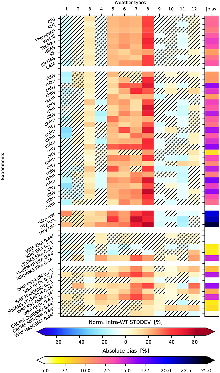
Figure 7. Similar to Figure 6 but showing the simulated divided by ERA-Interim intra-WT pattern standard deviations. A perfect score is zero and denotes that the model has the same variability than ERA-Interim.
The WRF36 simulations have less skill in simulating intra-WT STDDEV than the NA-CORDEX runs (Figure 7). However, in contrast to the WT frequency analysis above, ERA-Interim driven WRF36 simulations have clearly higher skill than CESM driven simulations. The sensitivity to the used physics options is small. The transition season WT5–8 shows significant and systematically too high STDDEVs whereas too low STDDEVs seldom occur. The largest biases are found for WT8 with some simulations overestimating the observed STDDEV by more than 60%. The same WTs also show too high STDDEVs in the NA-CORDEX simulations, especially for the GCM driven runs, but the biases are smaller and less systematic than in WRF36. The best performance is again found for NA-CORDEX ERA-Interim driven WRF simulations with absolute average biases of <5%.
The third and last skill score that we consider is the WT centroid correlation coefficient, which allows one to assess how well the spatial pattern of each WT variable is reproduced by the RCMs. Values close to one indicate a skillful simulation of observed WT centroid patterns. Also here, the NA-CORDEX simulations outperform the WRF36 runs and the selected physics only have a minor impact on the performance of WRF36 simulations (Figure 8). In the WRF36 simulations, the lowest skills are found for simulating PW patterns, which becomes emphasized by changing from ERA-Interim to CESM boundary conditions. Particularly low PW pattern correlations are seen for WT3 and WT8. WT10 has very low correlation coefficients for UV500 when ERA-Interim is downscaled. SLP patterns generally show the highest correlation coefficients.
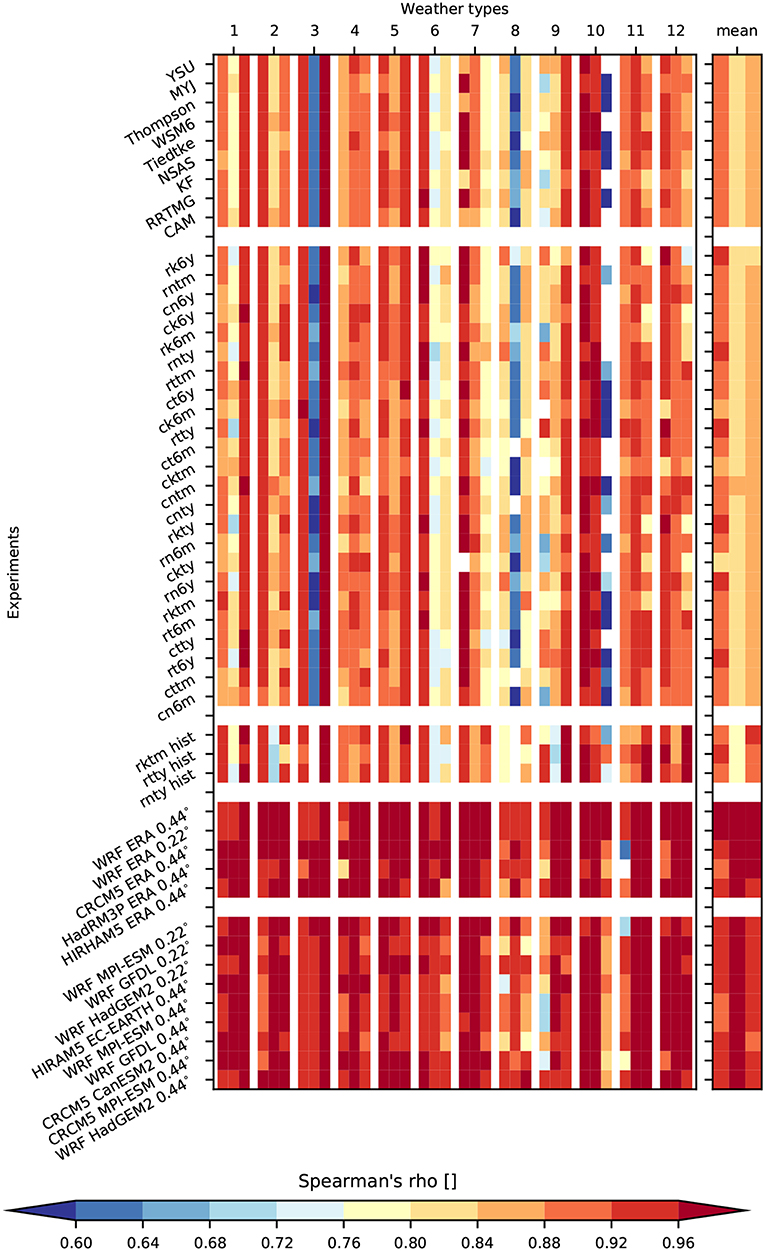
Figure 8. Similar to Figure 6 but showing correlation coefficients between ERA-Interim and simulated centroids (higher is better). Each column consists of three sub-columns showing correlation coefficients for SLP, PW, and 500 UV from left to right.
This is different in the NA-CORDEX simulations where PW patterns are simulated best. Again, ERA-Interim downscaled WRF simulations show the highest skills with average absolute values larger than 0.96. Simulated WT8 patterns have overall the lowest skill but most correlation coefficients are still larger than 0.88.
Here we summarize the origin of different performances in simulating WT characteristics with RCMs. The presented numbers are first-order estimates since a full variance analysis would demand many more simulations than are available, especially for the NA-CORDEX ensemble. Figure 9 shows the spread in the three assessed skill scores averaged over specific dimensions of the RCM ensembles.
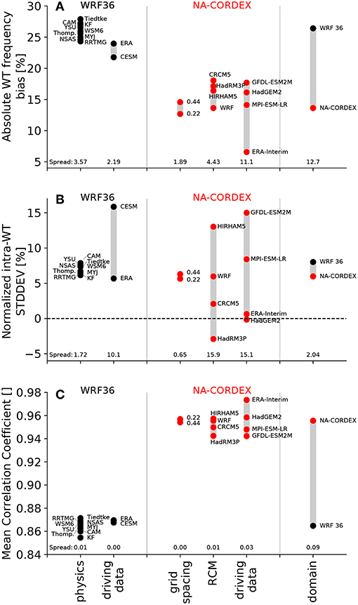
Figure 9. Estimates of WT skill variability for different drivers using three metrics: (A) absolute WT frequency biases, (B) normalized intra-WT standard deviations, and (C) mean centroid pattern correlation coefficients. The impact of model physics and driving data is investigated in the WRF36 simulations (black symbols). The effect of horizontal grid spacing, RCM, and driving data is assessed for the NA-CORDEX simulations (red symbols). The impact of the domain size is estimated comparing WRF simulations in the NA-CORDEX ensemble with WRF36 runs. The maximum minus minimum spread is shown on the bottom of each panel.
WT frequencies in WRF36 simulations are fairly similar for all ensemble members and only weakly depend on the model physics and driving data (only the RKTM, RNTY, and RTTY are compared for the latter; Figure 9A). The NA-CORDEX simulations show higher skill in simulating WT frequencies. The 0.22 horizontal grid spacing WRF NA-CORDEX simulations show 1.9% lower absolute average WT frequency biases compared to their 0.44 counterparts. There is moderate variability (4.4%) concerning the RCM formulation, with CRCM5 showing the highest biases and WRF the lowest. A large variability of 11.1% occurs due to the selected driving data with ERA-Interim clearly resulting in the lowest biases. WRF36 and WRF-NA-CORDEX simulations show substantial variability of 12.7%, which is likely caused by differences in domain size and the application of spectral nudging in the WRF NA-CORDEX, resulting in a more realistic representation of WTs in the latter.
The WRF36 intra-WT STDDEV shows small sensitivity to the model physics but large sensitivity (10.1%) to the driving data with ERA-Interim driven simulations showing clearly higher skill (Figure 9B). In the NA-CORDEX ensemble, the WRF model resolution has only minor effects on the skill but the RCM formulation plays a major role (15.9%). The HIRHAM simulations overestimate the STDDEV substantially while HadGEM3P and CRCM5 show high skill. Additionally, the driving GCM has a major impact (15.1%) with ERA-Interim and HadGEM2, resulting in very small biases and GFDL-ESM2M driven simulations resulting in large overestimations of intra-WT STDDEVs. Comparing the WRF simulations from the two ensembles results in similar skills. However, this is mainly due to the larger fraction of ERA-Interim driven members in the WRF36 ensemble (24 out of 27 runs) compared to the NA-CORDEX ensemble (two out of ten).
The average centroid correlation coefficients show very small sensitivities to the WRF36 model physics and driving data (Figure 9C). The different sources of variability in the NA-CORDEX simulations lead to only minor sensitivities, with the WRF grid spacing having the smallest impact and the driving GCM having the largest. The major mode of variability in this metric is the RCM domain size and the application of spectral nudging as shown by the difference in correlation coefficients between the WRF36 and WRF-NA-CORDEX simulations.
All GCM driven NA-CORDEX and WRF36 runs also provide future climate data that we use to assess if WT frequencies are projected to change due to climate change. The GCM driven NA-CORDEX simulations are transient climate runs that cover a common period from 1950 to 2099 (see Table 1) whereas the GCM driven WRF36 runs are time slice experiments that cover the periods 1990–2000, 2020–2030, 2030–2040, 2050–2060, and 2080–2090.
Most NA-CORDEX simulations show systematic increases in WT7 and WT8 frequencies by mid-century, which, however, are not statistically significant (Figure 10). WT2 and WT11 predominantly decrease in their frequency. Six out of the eleven simulations show significant decreases in WT11 frequencies. Most of the NA-CORDEX models still show increases in WT7 frequencies by the end of the century but more systematic and significant are the frequency increases in WT12, which were not obvious at mid-century. WT12 resembles monsoonal flow patterns and it is projected to increase in frequency in ten of eleven models. All NA-CORDEX models agree on a decrease of WT10 patterns by the end of the century, eight of them show systematic decreases, which would indicate a drying of the northern Great Plains during summer (Figure 4K). Furthermore, all models show decreases for WT4 frequencies, which are smaller in magnitude and only significant in three models. These systematic changes are likely a result of anthropogenic forcings such as increasing greenhouse gas emissions and changes in aerosol loads. Climate natural variability should have a minor impact because the NA-CORDEX ensemble is forced by various GCMs that each simulate differing phases of, e.g., ENSO or Pacific Decadal Oscillation.
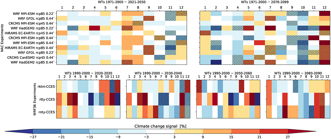
Figure 10. Heatmap showing WT frequency changes in future climate projections. The top panels show results from the NA-CORDEX ensemble using 1979–2000 as the baseline period and 2021–2050 (Left panel) and 2071–2100 (Right panel). The lower panels show results from the WRF36 CESM driven simulations with the baseline period 1990–2000 and the future periods 2020–2030, 2030–2040, 2050–2060, and 2080–2090 from left to right. Hatched boxes show changes that exceed the interannual variability in ERA-Interim.
WT frequency changes in the WRF36 ensemble are often not systematic and strongly vary from period to period. This is likely a result of the 11-year long time-slice experiments that are too short to differentiate between climate internal variability and forces climate change (Deser et al., 2012). Differences in the response of the CESM GCM, which is downscaled in the WRF36 ensemble, to the NA-CORDEX GCMs are unlikely but cannot be excluded.
In this study, we use two sets of RCM ensembles, the North American CORDEX (NA-CORDEX) ensemble and a perturbed WRF physics ensemble with 36 km horizontal grid spacing (WRF36). We use a weather typing (WTing) algorithm to investigate if RCM simulations are able to capture hydrologically important weather pattern characteristics over the CONUS. We investigate three metrics: (1) the frequency biases of WT occurrences; (2) the variability of flow patterns within WTs; and (3) the accurate representation of WT spatial patterns.
The NA-CORDEX ensemble clearly outperforms the WRF36 simulations in all three metrics but particularly in the first and third ones. The main source for WRF model skill differences is the size of the RCM domain and the application of spectral nudging. The WRF36 simulations have a much larger domain and do not use spectral nudging, which allows them to significantly deviate from their lateral boundary conditions on synoptic scales. The much smaller NA-CORDEX domains constrain synoptic patterns from the GCM in the RCM domain and result in a more skillful representation of WT characteristics, particularly when they are driven by reanalysis data. Previous research showed that the interior large-scale dynamics can start to depart from the driving data as domain size increases (Alexandru et al., 2007). The second metric shows a larger sensitivity to the driving model and the formulation of the RCM. Also in this metric, however, ERA-Interim driven NA-CORDEX simulations have clearly higher skill than the ERA-Interim driven WRF36 runs. WT characteristics have very little sensitivity to the model physics, which is a robust result from the WRF36 ensemble evaluation. Model physics are, however, very important when it comes to the simulation of mesoscale processes in the RCMs as shown by Mooney et al. (2017) and Bruyère et al. (2017).
Biases that are present in the simulation of WTs directly translate into biases in the representation of the hydrology in RCMs (e.g., Addor et al., 2016). For example, in this study most RCMs underestimate the frequency of WT4 patterns. Days within this pattern result in high precipitation rates in the Deep South and Appalachian region during winter. Too infrequent WT4 conditions result in cold-season conditions that are too dry in these regions. Besides the biases in WT characteristics, RCMs also have biases in the representation of smaller-scale processes such as microphysics or mesoscale dynamics that affect model quality. The presented WT analysis can help to distinguish these two sources of biases, which is not possible when RCMs are evaluated on, for example, a seasonal basis.
WTing applied to climate change projections allows for understanding changes in the synoptic-scale conditions that occur in parallel to thermodynamic changes. A better understanding of changes in the large-scale dynamics is important since almost all climate change signals that we have confidence in originate from thermodynamic changes (Shepherd, 2014). The 11-year-long time slice experiments from the WRF36 ensemble do not allow a robust assessment of climate change in WT frequencies since they are dominated by climate internal variability. However, eight of eleven transient NA-CORDEX simulations show statistically significant increases in North American Monsoonal circulation (WT12) and a statistically significant decrease in patterns that transport moisture into the Northern Plains and Rockies (WT10) during the early warm season. The increase in monsoonal flow is consistent with other studies (Bukovsky et al., 2015, 2017; Prein, under review), which used different types of climate model data and show that the monsoon high strengthens and sets in earlier in the season. The decrease in WT10 seems to be physically linked to the increase in monsoonal flow since southwest monsoon precipitation is anticorrelated with precipitation in the plains. This is due to the modulation of the low pressure influence in the plains (WT10) by the stronger and more persistent monsoon circulation in the future (WT12).
This study shows that the RCM domain size and the application of spectral nudging can have a significant impact on the model's ability to capture realistic large-scale dynamics in mid-latitudes. Previous work showed that at the very least, RCM lateral boundaries should be sufficiently far removed from the region of interest to minimize spatial spin-up issues (Leduc and Laprise, 2009; Brisson et al., 2015; Matte et al., 2017). In addition, the domain should capture any key contributing regional physical processes missing from the lateral boundary conditions (Giorgi and Mearns, 1999). For example, a regional study of North Atlantic tropical cyclones by Done et al. (2015) required a large domain to capture the development of African easterly waves within the RCM domain. Erfanian and Wang (2018) came to a similar conclusion and showed that including teleconnected oceanic regions in the RCM domain improves its performance. However, too large domains and/or a lack of spectral nudging can lead to biased synoptic-scale patterns as shown here. Therefore, modelers have to find a balance between spinning up mesoscale processes that are not affected by the lateral boundary conditions and simulating large-scale dynamics realistically.
The accurate simulation of synoptic-scale variability in the driving GCM is essential since correcting for such biases in the RCM is challenging (Diaconescu et al., 2007). In contrast, correcting thermodynamic biases in the lateral boundary conditions of the RCM is somewhat easier (Bruyère et al., 2014; Xu and Yang, 2015), although challenges remain (Rocheta et al., 2014). Selecting GCMs with well-simulated large-scale dynamics should be a high priority for RCM downscaling experiments. WTing algorithms, such as the one used here, can support such a model selection.
If the large-scale dynamics are accurately captured in the GCM, spectral nudging can help to constrain synoptic-scale processes in large-domain RCM simulation (von Storch et al., 2000). Care has to be taken that the nudging does not disturb the development of mesoscale structures that are simulated by the RCM.
Another solution would be to use variable resolution GCMs such as the ICOsahedral Non-hydrostatic model (ICON; Zängl et al., 2015) or the Model for Prediction Across Scales (MPAS; Skamarock et al., 2012) instead of limited area modeling for downscaling experiments. These models, in theory, should resolve the domain size dependence of simulating WTs although they are more expensive since they simulate the entire globe instead of a limited area.
Generally, RCMs from both ensembles have larger WT frequency biases for cold season WTs than warm season WTs. The overestimation of variability within shoulder season WTs is also systematic. Future studies should focus on understanding the reason for these systematic biases. Our analyses suggest that these biases are related to the RCM formulation (e.g., model numerics) more so than the model physics.
Future work should also investigate the drivers behind the forced decrease in WT10 and increase in WT12. The consistency of these changes among model projections is surprising since climate change impacts on large-scale dynamics are often uncertain (Shepherd, 2014). Understanding the underlying processes of these changes is important due to their potential impacts on the summertime climate of the U.S. Targeted GCM experiments such as constant soil moisture or constant ice-cover experiments could help to gain insights on the large-scale drivers while additional RCM downscaling could help to understand the regional and local scale impacts.
This study is limited due to the use of existing RCM ensemble datasets, which were not specifically designed to address the impacts of domain size or spectral nudging on large scale circulation patterns. A more systematic analysis that includes the evaluation of WTs in the driving GCMs, the impact of spectral nudging on large domains, and a more systematic perturbation of the RCM domain size would be necessary to fully understand the sources of differences between the NA-CORDEX and WRF36 ensemble. Such an analysis could also help to understand if RCMs are able to add value to the driving GCM's large-scale dynamics by simulating upscale effects of mesoscale processes, or if their added value is constrained to regional scales.
AP designed the study, performed the data analysis, and produced the figures. MB performed data processing of the NA-CORDEX simulations. CB led the development of the WRF36 ensemble. All authors contributed to discussions and helped writing the manuscript.
NCAR is primarily funded by the National Science Foundation. This work was supported by the NCAR Weather and Climate Impacts Assessment Science Program and Regional Climate Uncertainty Program funded by NSF under the NCAR cooperative agreement managed by LM. We are grateful to NCAR's Computational and Information Systems Laboratory (CISL) who granted computational resources on its Yellowstone: IBM iDataPlex System (Climate Simulation Laboratory) http://n2t.net/ark:/85065/d7wd3xhc to perform the WRF36 and parts of the NA-CORDEX simulations. Additionally, CISL provides storage for archiving both RCM ensembles on its GLADE file system.
The authors declare that the research was conducted in the absence of any commercial or financial relationships that could be construed as a potential conflict of interest.
We acknowledge ECMWF for providing access to its ERA-Interim reanalysis data. We also thank the PRISM Climate Group at Oregon State University for granting access to its daily gridded precipitation product. We acknowledge the World Climate Research Programme's Working Group on Regional Climate, and the Working Group on Coupled Modelling, former coordinating body of CORDEX and responsible panel for CMIP5. We also thank the climate modeling groups (listed in Table 1 of this paper) for producing and making available their model output. We also acknowledge the U.S Department of Defense ESTCP for its support of the NA-CORDEX data archive.
Addor, N., Rohrer, M., Furrer, R., and Seibert, J. (2016). Propagation of biases in climate models from the synoptic to the regional scale: implications for bias adjustment. J. Geophys. Res. Atmos. 121, 2075–2089. doi: 10.1002/2015JD024040
Alexandru, A., de Elia, R., and Laprise, R. (2007). Internal variability in regional climate downscaling at the seasonal scale. Mon. Weather Rev. 135, 3221–3238. doi: 10.1175/MWR3456.1
Brisson, E., Demuzere, M., and Van Lipzig, N. (2015). Modelling strategies for performing convection-permitting climate simulations. Meteorol. Z. 25, 149–163. doi: 10.1127/metz/2015/0598
Bruyère, C., Rasmussen, R., Gutmann, E., Done, J., Tye, M., Jaye, A., et al. (2017). Impact of Climate Change on Gulf of Mexico Hurricanes. Technical report, Technical Note NCAR/TN-535+ STR. NCAR.
Bruyère, C. L., Done, J. M., Holland, G. J., and Fredrick, S. (2014). Bias corrections of global models for regional climate simulations of high-impact weather. Clim. Dyn. 43, 1847–1856. doi: 10.1007/s00382-013-2011-6
Bruyère, C. L., Monaghan, A. J., Steinhoff, D. F., and Yates, D. (2015). Bias-Corrected CMIP5 CESM Data in WRF/MPAS Intermediate File Format (Boulder, CO: NCAR Technical Note NCAR/TN-515+STR), 27. doi: 10.5065/D6445JJ7
Bukovsky, M. S., Carrillo, C. M., Gochis, D. J., Hammerling, D. M., McCrary, R. R., and Mearns, L. O. (2015). Toward assessing NARCCAP regional climate model credibility for the North American monsoon: future climate simulations. J. Clim. 28, 6707–6728. doi: 10.1175/JCLI-D-14-00695.1
Bukovsky, M. S., McCrary, R. R., Seth, A., and Mearns, L. O. (2017). A mechanistically credible, poleward shift in warm-season precipitation projected for the US southern great plains? J. Clim. 30, 8275–8298. doi: 10.1175/JCLI-D-16-0316.1
Buonomo, E., Jones, R., Huntingford, C., and Hannaford, J. (2007). On the robustness of changes in extreme precipitation over Europe from two high resolution climate change simulations. Q. J. Royal Meteorol. Soc. 133, 65–81. doi: 10.1002/qj.13
Caya, D., and Laprise, R. (1999). A semi-implicit semi-Lagrangian regional climate model: the Canadian RCM. Mon. Weather Rev. 127, 341–362. doi: 10.1175/1520-0493(1999)127<0341:ASISLR>2.0.CO;2
Christensen, J. H., Carter, T. R., Rummukainen, M., and Amanatidis, G. (2007a). Evaluating the performance and utility of regional climate models: the PRUDENCE project. Clim. Change. 81, 1–6. doi: 10.1007/s10584-006-9211-6
Christensen, O. B., Drews, M., Christensen, J. H., Dethloff, K., Ketelsen, K., Hebestadt, I., et al. (2007b). The HIRHAM Regional Climate Model Version 5 (β). Techical Report, 6–17.
Clark, A. J., Gallus Jr., W. A., Xue, M., and Kong, F. (2010). Convection-allowing and convection-parameterizing ensemble forecasts of a mesoscale convective vortex and associated severe weather environment. Weather Forecast. 25, 1052–1081. doi: 10.1175/2010WAF2222390.1
Collins, W. D., Bitz, C. M., Blackmon, M. L., Bonan, G. B., Bretherton, C. S., Carton, J. A., et al. (2006). The community climate system model version 3 (CCSM3). J. Clim. 19, 2122–2143. doi: 10.1175/JCLI3761.1
Daly, C., Neilson, R. P., and Phillips, D. L. (1994). A statistical-topographic model for mapping climatological precipitation over mountainous terrain. J. Appl. Meteorol. 33, 140–158. doi: 10.1175/1520-0450(1994)033<0140:ASTMFM>2.0.CO;2
Decker, M., Brunke, M. A., Wang, Z., Sakaguchi, K., Zeng, X., and Bosilovich, M. G. (2012). Evaluation of the reanalysis products from GSFC, NCEP, and ECMWF using flux tower observations. J. Clim. 25, 1916–1944. doi: 10.1175/JCLI-D-11-00004.1
Dee, D. P., Uppala, S. M., Simmons, A., Berrisford, P., Poli, P., Kobayashi, S., et al. (2011). The ERA-interim reanalysis: configuration and performance of the data assimilation system. Q. J. Royal Meteorol. Soc. 137, 553–597. doi: 10.1002/qj.828
Delage, Y. (1997). Parameterising sub-grid scale vertical transport in atmospheric models under statically stable conditions. Bound. Layer Meteorol. 82, 23–48. doi: 10.1023/A:1000132524077
Denis, B., Laprise, R., Caya, D., and Côté, J. (2002). Downscaling ability of one-way nested regional climate models: the Big-Brother experiment. Clim. Dyn. 18, 627–646. doi: 10.1007/s00382-001-0201-0
Deser, C., Phillips, A., Bourdette, V., and Teng, H. (2012). Uncertainty in climate change projections: the role of internal variability. Clim. Dyn. 38, 527–546. doi: 10.1007/s00382-010-0977-x
Di Luca, A., de Elía, R., and Laprise, R. (2012). Potential for added value in precipitation simulated by high-resolution nested regional climate models and observations. Clim. Dyn. 38, 1229–1247. doi: 10.1007/s00382-011-1068-3
Diaconescu, E. P., Laprise, R., and Sushama, L. (2007). The impact of lateral boundary data errors on the simulated climate of a nested regional climate model. Clim. Dyn. 28, 333–350. doi: 10.1007/s00382-006-0189-6
Done, J. M., Holland, G. J., Bruyère, C. L., Leung, L. R., and Suzuki-Parker, A. (2015). Modeling high-impact weather and climate: lessons from a tropical cyclone perspective. Clim. Change. 129, 381–395. doi: 10.1007/s10584-013-0954-6
Doswell III, C. A., Brooks, H. E., and Maddox, R. A. (1996). Flash flood forecasting: an ingredients-based methodology. Weather Forecast. 11, 560–581. doi: 10.1175/1520-0434(1996)011<0560:FFFAIB>2.0.CO;2
Erfanian, A., and Wang, G. (2018). Explicitly accounting for the role of remote oceans in regional climate modeling of South America. J. Adv. Model. Earth Syst. 10, 2408–2426. doi: 10.1029/2018MS001444
Essery, R., and Clark, D. B. (2003). Developments in the MOSES 2 land-surface model for PILPS 2e. Glob. Planet. Change. 38, 161–164. doi: 10.1016/S0921-8181(03)00026-2
Feser, F., Rockel, B., von Storch, H., Winterfeldt, J., and Zahn, M. (2011). Regional climate models add value to global model data: a review and selected examples. Bull. Am. Meteorol. Soc. 92, 1181–1192. doi: 10.1175/2011BAMS3061.1
García-Valero, J. A., Montavez, J. P., Jerez, S., Gómez-Navarro, J. J., Lorente-Plazas, R., and Jiménez-Guerrero, P. (2012). A seasonal study of the atmospheric dynamics over the Iberian Peninsula based on circulation types. Theor. Appl. Climatol. 110, 291–310. doi: 10.1007/s00704-012-0623-0
Gibson, P. B., Uotila, P., Perkins-Kirkpatrick, S. E., Alexander, L. V., and Pitman, A. J. (2016). Evaluating synoptic systems in the CMIP5 climate models over the Australian region. Clim. Dyn. 47, 2235–2251. doi: 10.1007/s00382-015-2961-y
Giorgi, F. (1990). Simulation of regional climate using a limited area model nested in a general circulation model. J. Clim. 3, 941–963. doi: 10.1175/1520-0442(1990)003<0941:SORCUA>2.0.CO;2
Giorgi, F., and Mearns, L. O. (1999). Introduction to special section: regional climate modeling revisited. J. Geophys. Res. Atmos. 104, 6335–6352. doi: 10.1029/98JD02072
Goodess, C. M., and Palutikof, J. P. (1998). Development of daily rainfall scenarios for southeast Spain using a circulation-type approach to downscaling. Int. J. Climatol. 18, 1051–1083. doi: 10.1002/(SICI)1097-0088(199808)18:10<1051::AID-JOC304>3.0.CO;2-1
Han, J., and Pan, H.-L. (2011). Revision of convection and vertical diffusion schemes in the NCEP global forecast system. Weather Forecast. 26, 520–533. doi: 10.1175/WAF-D-10-05038.1
Hong, S.-Y., Dudhia, J., and Chen, S.-H. (2004). A revised approach to ice microphysical processes for the bulk parameterization of clouds and precipitation. Mon. Weather Rev. 132, 103–120. doi: 10.1175/1520-0493(2004)132<0103:ARATIM>2.0.CO;2
Hong, S.-Y., and Lim, J.-O. J. (2006). The WRF single-moment 6-class microphysics scheme (WSM6). J. Korean Meteor. Soc. 42, 129–151.
Hong, S.-Y., Noh, Y., and Dudhia, J. (2006). A new vertical diffusion package with an explicit treatment of entrainment processes. Mon. Weather Rev. 134, 2318–2341. doi: 10.1175/MWR3199.1
Hurrell, J. W., Holland, M. M., Gent, P. R., Ghan, S., Kay, J. E., Kushner, P. J., et al. (2013). The community earth system model: a framework for collaborative research. Bull. Am. Meteorol. Soc. 94, 1339–1360. doi: 10.1175/BAMS-D-12-00121.1
Janjić, Z. I. (1994). The step-mountain eta coordinate model: further developments of the convection, viscous sublayer, and turbulence closure schemes. Mon. Weather Rev. 122, 927–945. doi: 10.1175/1520-0493(1994)122<0927:TSMECM>2.0.CO;2
Jones, R., Murphy, J., and Noguer, M. (1995). Simulation of climate change over Europe using a nested regional-climate model. I: assessment of control climate, including sensitivity to location of lateral boundaries. Q. J. Royal Meteorol. Soc. 121, 1413–1449.
Kain, J. S., and Fritsch, J. M. (1990). A one-dimensional entraining/detraining plume model and its application in convective parameterization. J. Atmos. Sci. 47, 2784–2802. doi: 10.1175/1520-0469(1990)047<2784:AODEPM>2.0.CO;2
Knutti, R., Masson, D., and Gettelman, A. (2013). Climate model genealogy: generation CMIP5 and how we got there. Geophys. Res. Lett. 40, 1194–1199. doi: 10.1002/grl.50256
Kotlarski, S., Keuler, K., Christensen, O. B., Colette, A., Déqué, M., Gobiet, A., et al. (2014). Regional climate modeling on European scales: a joint standard evaluation of the EURO-CORDEX RCM ensemble. Geosci. Model Dev. 7, 1297–1333. doi: 10.5194/gmd-7-1297-2014
Leduc, M., and Laprise, R. (2009). Regional climate model sensitivity to domain size. Clim. Dyn. 32, 833–854. doi: 10.1007/s00382-008-0400-z
Leung, L. R., Qian, Y., and Bian, X. (2003). Hydroclimate of the western United States based on observations and regional climate simulation of 1981–2000. Part I: seasonal statistics. J. Clim. 16, 1892–1911. doi: 10.1175/1520-0442(2003)016<1892:HOTWUS>2.0.CO;2
Li, J., and Barker, H. (2005). A radiation algorithm with correlated-k distribution. Part I: local thermal equilibrium. J. Atmos. Sci. 62, 286–309. doi: 10.1175/JAS-3396.1
Lin, R., Zhou, T., and Qian, Y. (2014). Evaluation of global monsoon precipitation changes based on five reanalysis datasets. J. Clim. 27, 1271–1289. doi: 10.1175/JCLI-D-13-00215.1
Lin, Y.-L., Chiao, S., Wang, T.-A., Kaplan, M. L., and Weglarz, R. P. (2001). Some common ingredients for heavy orographic rainfall. Weather Forecast. 16, 633–660. doi: 10.1175/1520-0434(2001)016<0633:SCIFHO>2.0.CO;2
Lorente-Plazas, R., Montávez, J., Jimenez, P., Jerez, S., Gómez-Navarro, J., García-Valero, J., et al. (2015). Characterization of surface winds over the Iberian Peninsula. Int. J. Climatol. 35, 1007–1026. doi: 10.1002/joc.4034
Martynov, A., Laprise, R., Sushama, L., Winger, K., Šeparović, L., and Dugas, B. (2013). Reanalysis-driven climate simulation over CORDEX North America domain using the Canadian Regional Climate Model, version 5: model performance evaluation. Clim. Dyn. 41, 2973–3005. doi: 10.1007/s00382-013-1778-9
Matte, D., Laprise, R., Thériault, J. M., and Lucas-Picher, P. (2017). Spatial spin-up of fine scales in a regional climate model simulation driven by low-resolution boundary conditions. Clim. Dyn. 49, 563–574. doi: 10.1007/s00382-016-3358-2
Mearns, L. O., Arritt, R., Biner, S., Bukovsky, M. S., McGinnis, S., Sain, S., et al. (2012). The North American regional climate change assessment program: overview of phase I results. Bull. Am. Meteorol. Soc. 93, 1337–1362. doi: 10.1175/BAMS-D-11-00223.1
Mearns, L. O., McGinnis, S., Korytina, D., Arritt, R., Biner, S., Bukovsky, M., et al. (2017). The NA-CORDEX Dataset, Version 1.0. NCAR Climate Data Gateway, Boulder CO. doi: 10.5065/D6SJ1JCH
Mlawer, E. J., Taubman, S. J., Brown, P. D., Iacono, M. J., and Clough, S. A. (1997). Radiative transfer for inhomogeneous atmospheres: RRTM, a validated correlated-k model for the longwave. J. Geophys. Res. Atmos. 102, 16663–16682. doi: 10.1029/97JD00237
Mooney, P., Broderick, C., Bruyère, C., Mulligan, F., and Prein, A. (2017). Clustering of observed diurnal cycles of precipitation over the United States for evaluation of a WRF multiphysics regional climate ensemble. J. Clim. 30, 9267–9286. doi: 10.1175/JCLI-D-16-0851.1
Morcrette, J. J (1984), Parameterization of radiation in general atmospheric circulation models, Ph.D. thesis, Univ. des Sci. et Technol (Lille), 373.
Nordeng, T. E. (1994). Extended versions of the convective parametrization scheme at ECMWF and their impact on the mean and transient activity of the model in the tropics. Res. Depart. Tech. Memo. 206, 1–41.
Paredes, D., Trigo, R. M., Garcia-Herrera, R., and Trigo, I. F. (2006). Understanding precipitation changes in Iberia in early spring: weather typing and storm-tracking approaches. J. Hydrometeorol. 7, 101–113. doi: 10.1175/JHM472.1
Prein, A., Gobiet, A., Truhetz, H., Keuler, K., Goergen, K., Teichmann, C., et al. (2016a). Precipitation in the EURO-CORDEX 0.11° and 0.44° simulations: high resolution, high benefits? Clim. Dyn. 46, 383–412. doi: 10.1007/s00382-015-2589-y
Prein, A. F., Holland, G. J., Rasmussen, R. M., Clark, M. P., and Tye, M. R. (2016b). Running dry: the US Southwest's drift into a drier climate state. Geophys. Res. Lett. 43, 1272–1279. doi: 10.1002/2015GL066727
Radić, V., and Clarke, G. K. (2011). Evaluation of IPCC models' performance in simulating late-twentieth-century climatologies and weather patterns over North America. J. Clim. 24, 5257–5274. doi: 10.1175/JCLI-D-11-00011.1
Rocheta, E., Evans, J. P., and Sharma, A. (2014). Assessing atmospheric bias correction for dynamical consistency using potential vorticity. Environ. Res. Lett. 9:124010. doi: 10.1088/1748-9326/9/12/124010
Rummukainen, M. (2010). State-of-the-art with regional climate models. Wiley Interdiscip. Rev. Clim. Change. 1, 82–96. doi: 10.1002/wcc.8
Rummukainen, M. (2016). Added value in regional climate modeling. Wiley Interdiscip. Rev. Clim. Change. 7, 145–159. doi: 10.1002/wcc.378
Santos, J. A., Belo-Pereira, M., Fraga, H., and Pinto, J. G. (2016). Understanding climate change projections for precipitation over western Europe with a weather typing approach. J. Geophys. Res. Atmos. 121, 1170–1189. doi: 10.1002/2015JD024399
Schiemann, R., and Frei, C. (2010). How to quantify the resolution of surface climate by circulation types: an example for Alpine precipitation. Phys. Chem. Earth. 35, 403–410. doi: 10.1016/j.pce.2009.09.005
Šeparović, L., Alexandru, A., Laprise, R., Martynov, A., Sushama, L., Winger, K., et al. (2013). Present climate and climate change over North America as simulated by the fifth-generation Canadian regional climate model. Clim. Dyn. 41, 3167–3201. doi: 10.1007/s00382-013-1737-5
Shepherd, T. G. (2014). Atmospheric circulation as a source of uncertainty in climate change projections. Nat. Geosci. 7:703. doi: 10.1038/ngeo2253
Skamarock, W. C., and Klemp, J. B. (2008). A time-split nonhydrostatic atmospheric model for weather research and forecasting applications. J. Comput. Phys. 227, 3465–3485. doi: 10.1016/j.jcp.2007.01.037
Skamarock, W. C., Klemp, J. B., Duda, M. G., Fowler, L. D., Park, S.-H., and Ringler, T. D. (2012). A multiscale nonhydrostatic atmospheric model using centroidal Voronoi tesselations and C-grid staggering. Mon. Weather Rev. 140, 3090–3105. doi: 10.1175/MWR-D-11-00215.1
Straus, D. M., and Molteni, F. (2004). Circulation regimes and SST forcing: results from large GCM ensembles. J. Clim. 17, 1641–1656. doi: 10.1175/1520-0442(2004)017<1641:CRASFR>2.0.CO;2
Sundqvist, H. (1978). A parameterization scheme for non-convective condensation including prediction of cloud water content. Q. J. Royal Meteorol. Soc. 104, 677–690. doi: 10.1002/qj.49710444110
Taylor, K. E., Stouffer, R. J., and Meehl, G. A. (2012). An overview of CMIP5 and the experiment design. Bull. Am. Meteorol. Soc. 93, 485–498. doi: 10.1175/BAMS-D-11-00094.1
Tewari, M., Chen, F., Wang, W., Dudhia, J., LeMone, M., Mitchell, K., et al. (2004). “Implementation and verification of the unified NOAH land surface model in the WRF model.” in 20th Conference on Weather Analysis and Forecasting/16th Conference on Numerical Weather Prediction (Seattle, WA). Vol. 1115.
Thompson, G., Rasmussen, R. M., and Manning, K. (2004). Explicit forecasts of winter precipitation using an improved bulk microphysics scheme. Part I: description and sensitivity analysis. Mon. Weather Rev. 132, 519–542. doi: 10.1175/1520-0493(2004)132<0519:EFOWPU>2.0.CO;2
Tiedtke, M. (1989). A comprehensive mass flux scheme for cumulus parameterization in large-scale models. Mon. Weather Rev. 117, 1779–1800. doi: 10.1175/1520-0493(1989)117<1779:ACMFSF>2.0.CO;2
van Bebber, W. J. (1891). Die Wettervorhersage: Eine praktische Anleitung zur Wettervorhersage auf Grundlage der Zeitungswetterkarten und Zeitungswetterberichte, für alle Berufsarten. Enke.
Van Vuuren, D. P., Edmonds, J., Kainuma, M., Riahi, K., Thomson, A., Hibbard, K., et al. (2011). The representative concentration pathways: an overview. Clim. Change. 109:5. doi: 10.1007/s10584-011-0148-z
Verseghy, D. (2009). CLASS–The Canadian Land Surface Scheme (Version 3.4) Technical Documentation (Version 1.1), Environment Canada. Downsview, ON: Climate Research Division, Science and Technology Branch.
Verseghy, D. L. (1991). CLASS–a Canadian land surface scheme for GCMs. I. Soil model. Int. J. Climatol. 11, 111–133. doi: 10.1002/joc.3370110202
von Storch, H., Langenberg, H., and Feser, F. (2000). A spectral nudging technique for dynamical downscaling purposes. Mon. Weather Rev. 128, 3664–3673. doi: 10.1175/1520-0493(2000)128<3664:ASNTFD>2.0.CO;2
Wood, J., Harrison, S., Turkington, T., and Reinhardt, L. (2016). Landslides and synoptic weather trends in the European Alps. Clim. Change. 136, 297–308. doi: 10.1007/s10584-016-1623-3
Xu, Z., and Yang, Z.-L. (2015). A new dynamical downscaling approach with GCM bias corrections and spectral nudging. J. Geophys. Res. Atmos. 120, 3063–3084. doi: 10.1002/2014JD022958
Zadra, A., Caya, D., Côté, J., Dugas, B., Jones, C., Laprise, R., et al. (2008). The next Canadian regional climate model. Phys. Can. 64, 75–83.
Keywords: regional climate models, uncertainties, weather types, North America, CORDEX, domain size, driving data, model quality
Citation: Prein AF, Bukovsky MS, Mearns LO, Bruyère CL and Done JM (2019) Simulating North American Weather Types With Regional Climate Models. Front. Environ. Sci. 7:36. doi: 10.3389/fenvs.2019.00036
Received: 23 November 2018; Accepted: 28 February 2019;
Published: 10 April 2019.
Edited by:
Hans Von Storch, Helmholtz Centre for Materials and Coastal Research (HZG), GermanyReviewed by:
Juan Pedro Montávez, University of Murcia, SpainCopyright © 2019 Prein, Bukovsky, Mearns, Bruyère and Done. This is an open-access article distributed under the terms of the Creative Commons Attribution License (CC BY). The use, distribution or reproduction in other forums is permitted, provided the original author(s) and the copyright owner(s) are credited and that the original publication in this journal is cited, in accordance with accepted academic practice. No use, distribution or reproduction is permitted which does not comply with these terms.
*Correspondence: Andreas F. Prein, cHJlaW5AdWNhci5lZHU=
Disclaimer: All claims expressed in this article are solely those of the authors and do not necessarily represent those of their affiliated organizations, or those of the publisher, the editors and the reviewers. Any product that may be evaluated in this article or claim that may be made by its manufacturer is not guaranteed or endorsed by the publisher.
Research integrity at Frontiers
Learn more about the work of our research integrity team to safeguard the quality of each article we publish.