Sensitivity Analysis of Some Key Factors on Turbulence Models for Hydrogen Diffusion Using HYDRAGON Code

In this paper, we have investigated the influence of air-fountain injection to study the hydrogen diffusion behavior with the help of 3-Dimensional code, HYDRAGON. Three different turbulence models i. e., Standard k −, model, Re-Normalized Group k − m model and Realizable k − e model have been studied carefully and the comparison of simulated data with experimental data were performed. The effect of air-injection was examined using three different velocities i.e., 0.411, 2.803, and 5.143 m/s to evaluate the phenomena of stratification break-up. When we kept the velocity of the air-injection as low as 0.411 m/s, the simulated results obtained through these three turbulence models were very close to experimental data. As the velocity was set to 5.143 m/s, the simulated data captured the experimental data well. But, when the velocity of air-injection was kept 2.803 m/s, the two turbulence models i.e., SKE and RNG turbulence models gave satisfactory results. However, when we added the turbulent diffusivity coefficient to RNG and RLZ turbulence models in the HYDRAGON code, a minor influence was investigated in these simulation results.

Introduction

Due to oxidation and core degradation, a large amount of hydrogen is generated and released into the reactor containment during a severe accidental scenario in the nuclear power plant (NPP). The density of air is 14 times higher than hydrogen, and the flammability range of hydrogen is much higher. These distinct properties show that hydrogen may disperse tremendously faster during accidental conditions, and detonation or deflagration may be initiated inevitably by the potential ignition source. This may threaten the integrity and safety system of the reactor containment. The possible risk related to hydrogen was initially observed during the accident which occurred in Three Mile Island (TMI) in 1979. This was the first well-known example where combustion of hydrogen took place, and where an enormous quantity of hydrogen was generated as a consequence of steam-zirconium interaction in the fuel cladding (Abdalla et al., 2014; Saeed et al., 2016, 2017a,b; Huanga et al., 2017). The hydrogen detonation in the Fukushima Dai-ichi Nuclear Power Plant (NPP) accident (2011) was another example which compelled scientists to explore the risk of hydrogen detonation during a severe accident. Both of these accidents indicate that modeling the gas behavior is an important subject of interest. To evaluate the combustion that would be detrimental to the reactor, hydrogen distribution must be modeled precisely to measure the initial conditions following combustion (Visser et al., 2012; Abdalla et al., 2015; Yang et al., 2017).

It is quite necessary to keep an eye on the hydrogen concentration during an accident scenario in the containment of an NPP to investigate the probable hydrogen risk and efficiency of the mitigation systems which are fixed in the containment of the NPP (Saeed et al., 2017a). In previous decades, scientists have developed two thermal-hydraulics approaches i.e., Lumped parameters (LP) and computational fluid dynamics (CFD) codes to simulate the related problems in the reactor core (Prabhudharwadkar et al., 2011; Xiao and Travis, 2013). In the beginning, LP codes such as MAAP and CONTAIN were used to predict the hydrogen safety behavior in the NPP (Kanzleiter and Fischer, 1994). For predicting the average hydrogen concentration in the containment, the LP method is more effective for predicting a longer duration of simulation because of its fast estimation for the hydrogen distribution. This method was more effective to investigate the average hydrogen concentration and it could not provide any estimation about the local distribution inside a compartment. Therefore, high-resolution CFD codes were presented for predicting the distribution of hydrogen at low spatial scales. The CFD largely has enhanced the precision, accuracy and analysis of the release of the hydrogen (Kanzleiter and Fischer, 1994; Heck et al., 1995; Bart et al., 2002; Visser et al., 2012).

Recently, 3D CFD codes such as ADREA-HF, CFD-ACE GOTHIC, REACFLOW, TONUS, CFX-5.7, GASFLOW, ROMs, and FLCAS etc. have been used for containment and industrial analyses. GOTHIC either deals with the LP computations or other systematic multidimensional assessment. Royl et al. (2000) used GASFLOW to predict the influence of combustion and hydrogen-steam distribution analysis in the konvoi-type NPP (Royl et al., 2000; Analytis, 2003; Grunloh and Manera, 2016). Houkema et al. (2008) performed a detail comparison between simulation results obtained from the LP code and commercial CFD code CFX and it was observed that a comprehensive three-dimensional analysis was necessary to get a local hydrogen distribution concentration (Houkema et al., 2008). A Russian type Water-Water-Energy-Reactor, VVER 440-213, was designed to perform simulations. Although these codes provided a certain degree of hydrogen mitigation, precise comparison of local hydrogen concentration was still unavailable (Kim et al., 2007).

The development of computational tools that precisely measure the hydrogen mixed gases inside the containment is still an unsolved issue. The precise measurement of the behavior of these gas species was a major concern for nuclear safety experts (Studer et al., 2012). Turbulence modeling is one of the important components to simulate gas mixing and transport equations. Different turbulence models (i.e., standard k − ε (hereafter SKE) turbulence model, re-normalization group k − ε (hereafter RNG) turbulence model, realizable k − ε (hereafter RLZ) turbulence model etc.) were used (Xiao and Travis, 2013; Zhang et al., 2015).

We studied the experimental work from Deri et al. (2010), and compared their experimental data with our simulation results obtained from HYDRAGON code (Abdalla, 2015; Saeed et al., 2016, 2017a,b; Zhang et al., 2017). For the current paper, the published data of the air-fountain case (air-fountain in the erosion of gaseous stratification) performed by Deri et al. was selected as a benchmark. To prevent the hydrogen risk combustion, helium was used during the experiment.

This work assesses the capability of the HYDRAGOON code to simulate the hydrogen distribution which is released during an accidental scenario in the containment of the NPP. In addition, this work is an important framework for assessment of hydrogen risk and risk reduction in the scenario of a severe accident at NPP. The major application of the HYDRAGON code is predicting the hydrogen behavior and multiple gas species inside the containment of NPP during a severe accident.

Numerical Methodology

The 3D HYDRAGON code was used for numerical simulation in this manuscript. The next sections of our report introduce the governing equations, various k − ε turbulence models i.e., SKE, RNG, and RLZ turbulence models, facility description and the initial and boundary conditions, in sequence.

Governing Equations

The governing equations used in this article are the viva unsteady average Navier-Stokes equations having mass and momentum conservation equations with turbulence transport equations. It is important to mention that the Navier-Stokes equations embody the physics of all types of fluid flows, including turbulent flow. The computations were initiated with three-dimensional transient simulations. The fluid properties such as velocity, pressure, temperature, etc. for the multicomponent fluid have been resolved by using the transport equations (Abdalla et al., 2015; Zhang et al., 2015, 2017; Saeed et al., 2016).

The transport equation is given as under:

$\begin{array}{ll}\frac{\partial (\rho Y_i)}{\partial t}+\nabla ·({\rho }_{\alpha }U{Y}_i)=-\nabla ·{\overrightarrow{J}}_i+S_i& (1)\end{array}$

where ρ represents the fluid density, ${\overrightarrow{J}}_i$ represent the diffusion flux, Y denotes mass fraction of gas species, U is used for the fluid velocity vector and S_i represents the conserved mass. Summation of mass fraction for each mixture component i is obtained as following.

$\begin{array}{ll}{{\displaystyle \sum }}_i^{NC}{Y}_i=1& (2)\end{array}$

where NC represents the number of components i.

Diffusion flux:

$\begin{array}{ll}{\overrightarrow{J}}_i=-\rho D_i\overrightarrow{\nabla }{Y}_i-\frac{{\mu }_t}{s{c}_t}\overrightarrow{\nabla }{Y}_i& (3)\end{array}$

where ${\overrightarrow{J}}_i$ represents the diffusion flux, ρ and D_i denote the fluid density of mixture of gas and mass diffusion, respectively. The term Y_i is the mass fraction for gas species i.

Continuity mass equation:

$\begin{array}{ll}\frac{\partial \rho }{\partial t}+\nabla .(\rho U)=0& (4)\end{array}$

Conservation of momentum:

$\begin{array}{ll}\frac{\partial (\rho U)}{\partial t}+\nabla .(\rho UU)=-\nabla P+\nabla .\tau +\rho g& (5)\end{array}$

where U and ρg represent the velocity vector and gravitational body force, respectively.

Stress tensor:

$\begin{array}{ll}\tau ={\mu }_{eff}\left(\nabla U-\frac{2}{3}\rho kI\right)& (6)\end{array}$

Effective turbulence viscosity:

$\begin{array}{ll}{\mu }_{eff}=\mu +{\mu }_T& (7)\end{array}$

where μ_eff is the effective turbulence viscosity, μ is the molecular viscosity and μ_T represents the turbulent viscosity.

Thermodynamic equation:

$\begin{array}{ll}p=z(\rho ,T)\rho \frac{R}{M}T& (8)\end{array}$

where R and M represent the universal gas constant and fluid molecular weight, respectively. The term z represents the compressibility; T represents the fluid absolute temperature and p represents pressure.

Density of the gas mixture:

$\begin{array}{ll}\frac{1}{\rho }=\frac{Y_{air}}{{\rho }_{air}}+\frac{Y_{helium}}{{\rho }_{helium}}& (9)\end{array}$

Molecular viscosity:

$\begin{array}{ll}\mu \left(T\right)=c_1{\left(\frac{T}{c_2}\right)}^{1.5}\times \frac{c_2+110.4}{T+110.4}& (10)\end{array}$

Turbulence Models

The two characteristic equations of N-S models i.e., mass, momentum, and energy equations are not closed. The process of closing the system of mean flow equations during computational system is known as turbulence modeling. Turbulence models are used to close the Reynolds stress term in the system of non-linear equations (Xie et al., 2008; Latif et al., 2013).

Turbulent kinetic energy:

$\begin{array}{ll}k=\frac{1}{2}\left(\overline{U^{\prime }.U^{\prime }}\right)& (11)\end{array}$

Dissipation rate:

$\begin{array}{ll}\epsilon =\nabla .(\upsilon U^{\prime }{U}^{\prime })& (12)\end{array}$

Turbulent Production:

$\begin{array}{ll}{p}_k={\mu }_t\left[\frac{\partial u_i}{\partial x_j}\left(\frac{\partial u_i}{\partial x_j}+\frac{\partial u_j}{\partial x_i}\right)\right]& (13)\end{array}$

Turbulent production of due to buoyancy effect:

$\begin{array}{ll}{G}_k=-g_i\frac{{\mu }_t}{\rho {Pr}_t}\frac{\partial \rho }{\partial x_i}& (14)\end{array}$

In the above equations, μ_t represents eddy viscosity, ρ is the density and p_rt is the turbulent Prandtl number. The vaule of turbulent Prandtl number was kept as 0.9.

The Standard k − ε turbulence model (Abdalla et al., 2014; Saeed et al., 2016)

Eddy viscosity:

$\begin{array}{ll}{\mu }_t=C_{\mu }\rho \frac{k^2}{\epsilon }& (15)\end{array}$

Transport equations of the SKE turbulence model:

$\begin{array}{l}\frac{\partial \left(\rho k\right)}{\partial t}+\frac{\partial }{\partial x_i}\left(\rho k{u}_i\right)=\\ \frac{\partial }{\partial x_j}\left[\left(\mu +\frac{{\mu }_t}{{\sigma }_k}\right)\frac{\partial k}{\partial x_j}\right]+P_k+G_k-\rho \epsilon & (16)\end{array}$

$\begin{array}{l}\frac{\partial \left(\rho \epsilon \right)}{\partial t}+\frac{\partial }{\partial x_i}\left(\rho \epsilon u_i\right)=\\ \frac{\partial }{\partial x_j}\left[\left(\mu +\frac{{\mu }_t}{{\sigma }_{\epsilon }}\right)\frac{\partial \epsilon }{\partial x_j}\right]+C_1\frac{\epsilon }{k}\left(P_k+G_k\right)-C_2\rho \frac{{\epsilon }^2}{k}& (17)\end{array}$

The model constants determined from simple benchmark are

C_u = 0.0, σ_k = 1.0, Pr = 0.85, C_ε1 = 1.44, C_ε2 = 1.92, σ_ε = 1.3

The RNG k − ε model equations are given as (Abdalla et al., 2014; Saeed et al., 2016).

Eddy viscosity:

$\begin{array}{ll}{\mu }_t=C_{\mu }\rho \frac{k^2}{\epsilon }& (18)\end{array}$

Transport equations of the RNG turbulence model:

$\begin{array}{l}\frac{\partial (\rho k)}{\partial t}+\frac{\partial }{\partial x_i}(\rho k{u}_i)=\\ \frac{\partial }{\partial x_j}\left[{\sigma }_k(\mu +{\mu }_t)\frac{\partial k}{\partial x_j}\right]+P_k+G_k-\rho \epsilon & (19)\end{array}$

$\begin{array}{l}\frac{\partial (\rho \epsilon )}{\partial t}+\frac{\partial (\rho \epsilon u_i)}{\partial x_i}=\\ \frac{\partial }{\partial x_j}\left[(\mu +{\mu }_t){\sigma }_{\epsilon }\frac{\partial \epsilon }{\partial x_j}\right]+C_{1RNG}\frac{\epsilon }{k}(P_k+G_k)-C_2\rho \frac{{\epsilon }^2}{k}& (20)\end{array}$

The model constants determined from simple benchmark are

C_u = 0.0, σ_k = 1.0, Pr = 0.85, C_ε1 = 1.44, C_ε2 = 1.92, σ_ε = 1.3

The Realizable k − ε model equations are (Abdalla et al., 2014; Saeed et al., 2016).

Transport equations of the RLZ turbulence model:

$\begin{array}{l}\frac{\partial \left(\rho k\right)}{\partial t}+\frac{\partial }{\partial x_i}\left(\rho k{u}_i\right)=\\ \frac{\partial }{\partial x_j}\left[\left(\mu +\frac{{\mu }_t}{{\sigma }_k}\right)\frac{\partial k}{\partial x_j}\right]+P_k+G_k-\rho \epsilon & (21)\end{array}$

$\begin{array}{l}\frac{\partial \left(\rho \epsilon \right)}{\partial t}+\frac{\partial \left(\rho \epsilon u_i\right)}{\partial x_i}=\\ \frac{\partial }{\partial x_j}\left[\left(\mu +\frac{{\mu }_t}{{\sigma }_{\epsilon }}\right)\frac{\partial \epsilon }{\partial x_j}\right]+C_1\rho S\epsilon +C_{1\epsilon }\frac{\epsilon }{k}{P}_k\\ -C_2\rho \frac{{\epsilon }^2}{k+\sqrt{\upsilon \epsilon }}& (22)\end{array}$

The model constants are

σ_ε = 1.2, C_1ε = 1.44, C₂ = 1.9.

Facility Description

The facility consisted of a parallelepiped, whose dimensions are 1.92 × 0.92 × 0.92 m (Height, length, and width) as shown in Figure 1. The inlet is located exactly in the middle of the bottom of the facility, and the outlet measuring 0.06 m is positioned at the bottom of the facility as shown in Figure 1. Initially, the facility was filled with air, and 9.1 g of helium was injected in via two upper inlets that were facing horizontally into the facility, during the initial 300 s of the simulation beginning. The air-injection was also started 1 min after the helium injection via the vertical nozzles that were positioned at 0.3 m from the roof on the lateral edges. The injection of air was continued for 300 s. To keep the pressure constant, the surpassing gas flowed out of the facility during the air-fountain. The sensor probes P1, P2, P3, P4, P5, and P6 were located 1.29, 1.09, 0.96, 0.83, 0.69, and 0.49 m, respectively from bottom of the enclosure as shown in Figure 1.

FIGURE 1

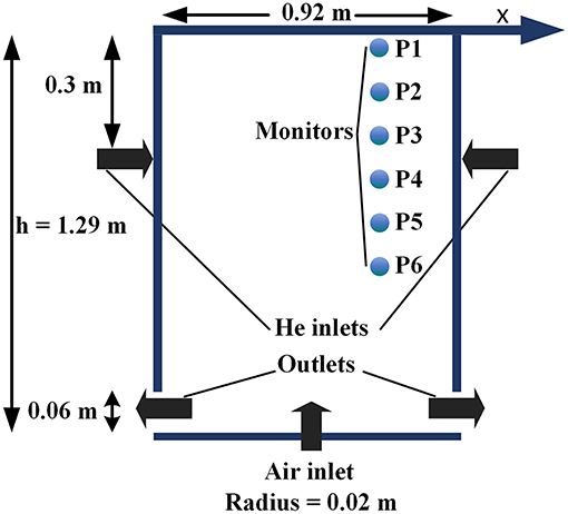
Figure 1. Sketch of the experimental layout.

Various Froude numbers (Fr) i.e., 0.16, 1.09, and 2.0 were applied to the experiment work to check the behavior of the penetrating jet deal during the experiment. The corresponding air-injections were 0.411, 2.803, and 5.143 m/s (Deri et al., 2010). Local Froude numbers were derived as a function of air-fountain reference velocity U_reff = 0.126 U_em/s, length scale of air-fountain L = 0.162 m, Brunt-Vaisala frequency N and stratification thickness H = 0.4 m. Design parameters of the layout is shown in Table 1.

$\begin{array}{llll}Fr& =& \frac{U_{reff}}{NL}& (23)\end{array}$

$\begin{array}{llll}N& =& {\left[\frac{2g}{{\rho }_1+{\rho }_2}\frac{{\rho }_1-{\rho }_2}{H}\right]}^{0.5}=2\left[s^{-1}\right]& (24)\end{array}$

where, N is known as Brunt-Vaisala frequency, used to define the initial condition for the stratification, ρ₁ is the density of the bottom zone, ρ₂ is the density of the upper zone, U_e is the air-fountain velocity and g is the gravity force.

TABLE 1

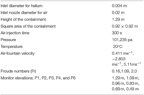
Table 1. Design parameters of the layout.

Initial and Boundary Conditions

To decrease the simulation duration and simplify the computation, we have simplified the geometry as a 3D quarter size. We have imposed a symmetry condition for the entire area and we have performed similar simulations in the other area. During the simulation, an adiabatic heat transfer with an isotropic system was applied. The air was injected through a square inlet whose dimension was 0.0088226917 × 0.0088226917 m. The whole simulations were divided into two different time steps. The duration of air-injection was 150–450 s following the start of the simulations. During the air-injection phase of simulation, when the velocity was high and constant, small time steps were adopted for solving the transient equation because of the higher turbulence intensity closer to the air-fountain source. In the latter phase, variable time steps were used as variation occurred in the velocity and became uncertain. Moreover, “time step maximal variation” was set at low levels. The simulations were performed with a structure of Cartesian coarse mesh, and three different grids conducted for the sensitive analysis were as 6,750, 40,500, and 54,000. An average mesh size of 1.8 × 1.8 × 3.1, 1.8 × 1.8 × 2.3 and 4.5 × 4.5 × 5 cm were tested and it was observed that the coarse mesh (4.5 × 4.5 × 5 cm having a total number of 6,750 grids) was sufficient to capture the gas mixture flow phenomena.

To reduce the simulation time, all the simulation results presented in the paper were computed by using 4.5 × 4.5 × 5 cm average mesh size. The computational domain cells were 15 cells along both the x- and y-axis, and 30 cells along the z-axis. For capturing the rapid variation in the density gradient, the highest mesh density was employed near the air-fountain region during the air-injection. Figure 2 illustrates the grid system for the computational domain obtained by using HYDRAGON code to solve Navier-Stocks equations. In this article, three different velocities for air-injection were used i.e., 0.411, 2.83, and 5.11 m/s. The helium mass diffusion coefficient for the mixture was 7.35 × 10⁻⁵. The fully inlet flow was assumed having values calculated with flow physical properties as under (Prabhudharwadkar et al., 2011).

$\begin{array}{ll}{k}_{in}=0.001{U_{in}}^2& (25)\end{array}$

$\begin{array}{ll}{\epsilon }_{in}=\frac{c_{\mu }{k}_{in}^{\raisebox{1ex}{$3$}\!\left/ \!\raisebox{-1ex}{$2$}\right.}}{l_{in}}& (26)\end{array}$

$\begin{array}{ll}{l}_{in}=0.42y_p& (27)\end{array}$

FIGURE 2

Figure 2. Cartesian mesh used for the computation of air-fountain experimental benchmark.

Results and Discussion

As the density of helium is lower, so the helium molecules were constantly diffused inside the facility. These helium molecules are consistently deposited on the upper part of the enclosure inside the containment. The air-injection was started after 150 s following the initiation of the simulation. After 450 s, the helium-injection was cut off following the initiation of the simulation. The air injection mixed the atmospheric components of the enclosure and the excess gases were able to exit through the outlet which maintained the thermodynamic pressure on the enclosure. According to the flow type, whole simulations were performed in two different steps. During the air-fountain and helium injection, we have used closely timed steps to solve the transient equations because of the turbulence intensity closer to the air fountain source. So, during the release phase, a longer simulation time was needed for the air fountain. After the release phase, variable time steps were used. The maximal variation for the time steps was kept at lower levels. The simulated data presented in this paper are dimensionless density ρ_ref − ρ/ρ_ref vs. time for the six monitors i.e., P1, P2, P3, P4 P5, and P6.

Effect of Velocity Injection Parameters

The simulations were performed by using three different air-injection velocities 0.411, 2.83, and 5.11 m/s to analyze stratification break-up phenomena. To study the interaction between the three different air-fountain velocities and the stratification helium layer, the simulated data was compared with the experimental results calculated at various air-injection velocities mentioned earlier for the three turbulence models.

When the air-injection velocities were set to 0.411 m/s, the results achieved by using the HYDRAGON code for the three turbulence models were in better agreement as shown in Figures 3, 4. The simulation results of the monitors P1 and P2 were close to the experimental data for all the turbulence models during the initial stage of the simulation and a small over prediction was observed after 600 s following the initiation of the simulation. Similarly, for all the remaining three monitors, the simulation results obtained by using HYDRAGON code captured the experimental trend during the initial stage of simulations and a small over prediction was observed at the latter phase of the simulation due to lower density of the helium as shown in Figures 3, 4. The simulation results illustrate that the injected momentum had an influence on the mixing regimes. Mixing process was dominated by molecular diffusion when air-injection velocity was set to 0.411 m/s.

FIGURE 3

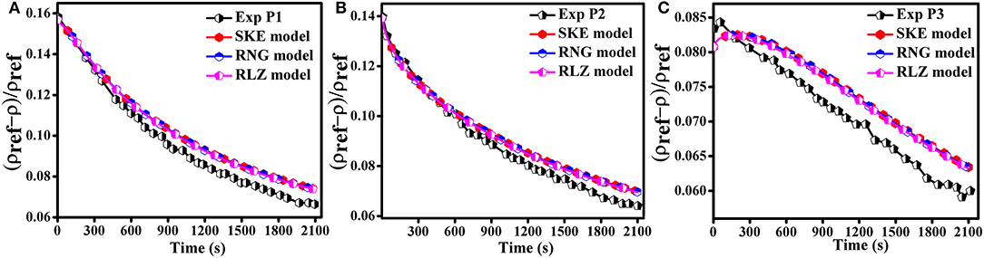
Figure 3. Effect of air-injection velocity 0.411 m/s on the simulation results for monitors (A) P1, (B) P2, and (C) P3.

FIGURE 4

Figure 4. Effect of air-injection velocity 0.411 m/s on the simulation results for monitors (A) P4, (B) P5, and (C) P6.

When the air-injection velocities were set to 2.83 m/s, the turbulence models choice had an influence on the simulation results.

The results obtained for the SKE and RNG turbulence models were closed to the experimental data, while discrepancies for the RLZ turbulence model were observed as shown in Figures 5, 6. The computational results of the RLZ turbulence model varied locally. The results of the RLZ turbulence model were underestimated for P1 and P2 and were improved for P3, P4, and P5, respectively.

FIGURE 5

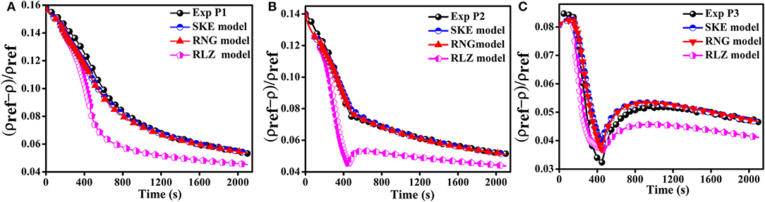
Figure 5. Effect of air-injection velocity 2.83 m/s on the simulation results for monitors (A) P1, (B) P2 and (C) P3.

FIGURE 6

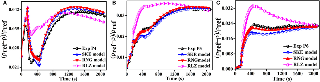
Figure 6. Effect of air-injection velocity 2.83 m/s on the simulation results for monitors (A) P4, (B) P5, and (C) P6.

The computational data achieved using SKE and RNG models were close to the experimental trend as compared to RLZ turbulence model at any area in the enclosure. Figures 5, 6 illustrate that the influence of the upward air fountain flow distance varied for all the three turbulence models. It was observed that the flow simulated by using the RLZ turbulence model reached a better trend than the other two turbulence models, and the horizontal spreading rate was also underestimated for the RLZ turbulence model. The SKE and RNG turbulence models generally better presented the predictions for the density stratification breakup phenomena.

The numerical results calculated when the air-injection was increased to 5.143 m/s for the three turbulence models are shown in Figures 7, 8. The momentum force derived the mixing when the air-injection was set to 5.143 m/s. When the air-injection velocity was set to 5.143 m/s, the simulation results obtained by the SKE turbulence model were similar to the simulation results obtained by RNG and RLZ turbulence models. In general, when air-injection velocity was set to 5.143 m/s, the three different turbulence models were in better agreement with experimental data as shown in Figures 7, 8.

FIGURE 7

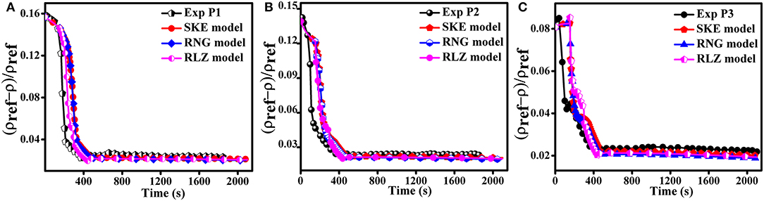
Figure 7. Effect of air-injection velocity 5.143 m/s on the simulation results for monitors (A) P1, (B) P2, and (C) P3.

FIGURE 8

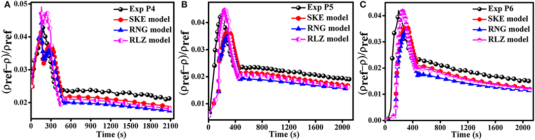
Figure 8. Effect of air-injection velocity 5.143 m/s on the simulation results for monitors (A) P4, (B) P5, and (C) P6.

Figure 9 compares the instantaneous mixture density distribution inside the containment for the SKE, RNG, and RLZ turbulence models computed by three various air-injection velocities, and the instantaneous results presented at 200 s. When air-injection velocity was very small, i.e., 0.411 m/s, the stratification layers were formed in-between the region where the helium concentration varied, as the helium concentrated at the upper part of the containment. When the air-injection velocity was increased to 2.803 m/s, stratification breakup was observed which was mainly caused by gravity driven force during the air-injection. If air-injection velocity was increased more up to 5.143 m/s, it suddenly penetrated the stratification layers and reached a higher distance but still was unable to penetrate helium stratification layer completely.

FIGURE 9

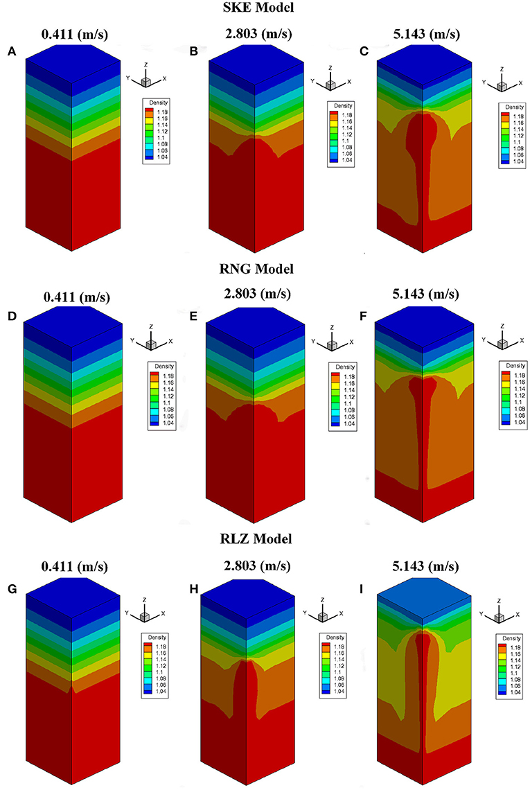
Figure 9. Comparison of instantaneous mixture density (kg/m³) calculated by three various air-injection velocities at 200 (s) for SKE (A) 0.411 m/s (B) 2.803 m/s (C) 5.143 m/s, RNG (D) 0.411 m/s (E) 2.803 m/s (F) 5.143 m/s, and RLZ (G) 0.411 m/s (H) 2.803 m/s (I) 5.143 m/s.

The comparison between the gravity-dominated and momentum-dominated regimes were observed by means of the interaction Froude number (Fr), which was set to 1 as a discriminating value. When Fr < 1, the momentum was overcome by the buoyancy and the air-injection was thus unable to penetrate the stratification. Actually, the air flow impinged over density surface and deflected downward with a fountain behavior.

Figures 10, 11 compared the instantaneous turbulence kinetic energy and dissipation rate, respectively for the SKE, RNG, and RLZ turbulence models calculated by three various air-injection velocities and the instantaneous results presented at 200 s. The simulation results illustrated that the air-injection momentum had large influence on the turbulence kinetic energy and dissipation rate. Largest turbulence kinetic energy and dissipation rate were observed when the air-injection velocity was increased to 5.143 m/s.

FIGURE 10

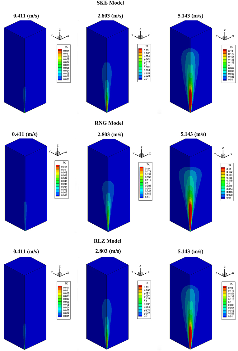
Figure 10. Comparison of instantaneous turbulence kinetic energy (m²/s²) calculated by three various air-injection velocities for SKE, RNG, and RLZ at 200 (s).

FIGURE 11

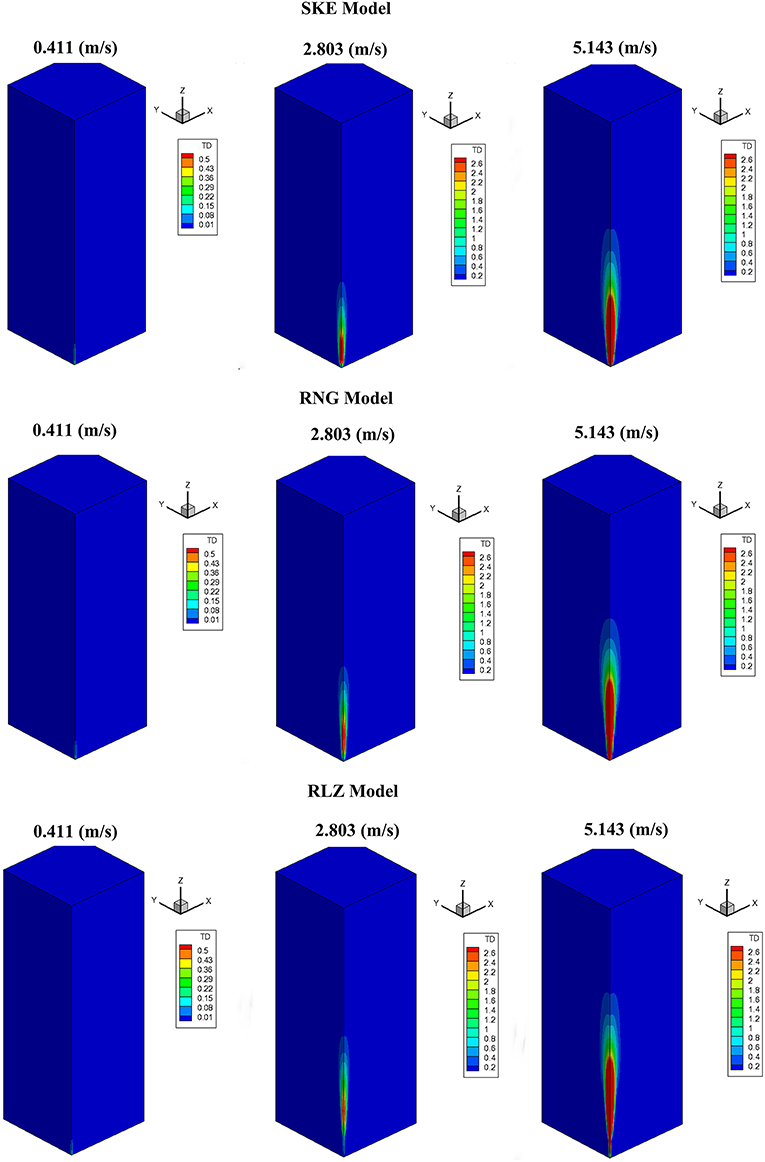
Figure 11. Comparison of instantaneous turbulence dissipation rate (m²/s³) calculated by three various air-injection velocities for SKE, RNG, and RLZ at 200 (s).

When, the injection was small, the molecular diffusion dominated the mixing. A buoyancy dominated mixing was observed, as the fountain flow rate was increased. When the value of Fr was set more than 1, the flow regime was momentum dominated and a rapid stratification break-up was observed.

Effect of Turbulent Diffusivity Term

The effect of the turbulent diffusivity was analyzed. The value of the turbulent Schmidt number Sc_t was set to 0.7 (Sanders et al., 1997) and the air-injection velocity was set to 2.83 m/s. Xiao and Travis (2013) suggested that value for the turbulent Schmidt number Sc_t can be selected in the range of 0.5–1.0 value. Figure 12 illustrates the comparison of simulation results calculated when turbulent diffusivity coefficient was included with the three turbulence models at P5 and P6 regions. Only the region near the air-fountain source was investigated, because it was the region where the turbulent diffusivity affected the most.

FIGURE 12

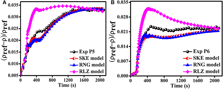
Figure 12. Effect of turbulent diffusivity on numerical results calculated for SKE, RNG, and RLZ for monitors (A) P5 and (B) P6, at inlet velocity 2.803 (m/s).

The simulation results illustrated that the turbulent diffusivity had a small effect on the simulation results at the region near air-fountain source i.e., P5 and P6, for the RNG and RLZ models and it did not have any noticeable effect on the SKE turbulence model as Figure 12. By including turbulent diffusivity term to the RNG model, it was observed that the simulation results agreed well with the simulation results obtained by RNG and RLZ model at the region near air-fountain source P6. The curves for the RNG and RLZ turbulence models were closer to the experimental trend when turbulent diffusivity was included to the HYDRAGON code. Moreover, turbulent diffusivity had no noticeable effect on the computed results obtained by SKE model as shown in Figure 12.

Conclusion

We have used three different velocities to investigate the stratification break-up phenomena. The molecular diffusion force caused the mixing process when the value of the velocity was 0.411 m/s. The gravity force was responsible for the mixing when the value of the air-injection was 2.803 m/s. The momentum forces derived from the mixing process as the air-injection was set to 5.143 m/s. The simulation results obtained by using various turbulence models showed that maximum penetration distance of the injected air-fountain varied for different turbulence models. It was observed that an air-injection did not have enough momentum to penetrate the helium stratification layer completely, where the injected air density was much heavier than the containment mixture. When the values of the air-injection velocities were 0.411 and 5.143 m/s, respectively, then the results achieved by these three turbulence models were closer to the experimental data. However, when 2.803 m/s velocity used, the results of SKE and RNG turbulence models were very close to the experimental trends at different points as compared to RLZ model. Furthermore, RNG model captured experimental trend better than SKE and RLZ models near the air-fountain source.

Furthermore, the effect of the turbulent diffusivity coefficient term was included to the k and ε equations. When we added the turbulent diffusivity coefficient term in the HYDRAGON code for RNG and RLZ turbulence models, a minor influence was observed in the results.

Data Availability Statement

All datasets generated for this study are included in the article/supplementary material.

Author Contributions

MS run simulations. XZho and JY have added turbulence models to the HYDRAGON code while XZha and AA helped in writing the paper.

Conflict of Interest

The authors declare that the research was conducted in the absence of any commercial or financial relationships that could be construed as a potential conflict of interest.

References

Abdalla, A. (2015). Validation of Turbulance Models for Gas Distribution Analysis Code (dissertation). Tsinghua University Beijing, Beijing, BJ, USA.

Abdalla, A., Yu, J., and Alrwashdeh, M. (2014). “Application of some turbulence models to simulate buoyancy-driven flow,” in Proceedings of the 2014 22nd International Conference on Nuclear Engineering (Prague: ASME Press).

Google Scholar

Abdalla, A., Yu, J., Chunhai, Z., Hou, B., and Saeed, M. (2015). “Investigation of the influence of turbulencemodels on the simulation of the gas distribution,” in Proceedings of the 23rd International Conference on Nuclear Engineering (Chiba: ASME Press).

Google Scholar

Analytis G. Th. (2003). Implementation of the renormalization group (RNG) k-ε turbulence model in GOTHIC/6.lb: solution methods and assessment. Ann. Nucl. Energy 30, 349–387. doi: 10.1016/S0306-4549(02)00061-0

CrossRef Full Text | Google Scholar

Bart, M., Dick, E., and Langhe, C. D. (2002). Application of an improved ε equation to a pilot jet diffusion flame. Combust Flame 131, 465–468. doi: 10.1016/S0010-2180(02)00420-0

CrossRef Full Text | Google Scholar

Deri, E., Cariteau, B., and Abdo, D. (2010). Air fountain in the erosion of gaseous stratification. Int. J. Heat Fluid Fl. 31:935. doi: 10.1016/j.ijheatfluidflow.2010.05.003

CrossRef Full Text | Google Scholar

Grunloh, T. P., and Manera, A. (2016). A novel domain overlapping strategy for the multiscale coupling of CFD with 1D system codes with applications to transient flows. Ann. Nucl. Energy 90, 442–432. doi: 10.1016/j.anucene.2015.12.027

CrossRef Full Text | Google Scholar

Heck, R., Kelber, G., Schmidt, K., and Zimmer, H. J. (1995). Hydrogen reduction following severe accidents using the dual recombiner-igniter concept. Nucl. Eng. Des. 157, 311–319. doi: 10.1016/0029-5493(95)01009-7

CrossRef Full Text | Google Scholar

Houkema, M., Siccama, N. B., Nijeholt, J. A., and Komen, E. M. J. (2008). Validation of the CFX4 CFD code for containment thermalhydraulics. Nucl. Eng. Des. 238, 590–599. doi: 10.1016/j.nucengdes.2007.02.033

CrossRef Full Text | Google Scholar

Huanga, T., Zhanga, Y., Tiana, W. X., Sua, G., and Qiua, S. Z. (2017). A 3-D simulation tool for hydrogen detonation during severe accident and its application. Ann. Nucl. Energy 104, 113–123. doi: 10.1016/j.anucene.2017.02.011

CrossRef Full Text | Google Scholar

Kanzleiter, T. F., and Fischer, K. O. (1994). Multi-compartment hydrogen deflagration experiments and model development. Nucl. Eng. Des. 146, 417–426. doi: 10.1016/0029-5493(94)90347-6

CrossRef Full Text | Google Scholar

Kim, J., Hong, S. W., Kim, S. B., and Kim, H. D. (2007). Three-dimensional behaviors of the hydrogen and steam in the APR1400 containment during a hypothetical loss of feed water accident. Ann. Nucl. Energy 34, 992–1001. doi: 10.1016/j.anucene.2007.05.003

CrossRef Full Text | Google Scholar

Latif, M., Masson, C., and Stathopoulos, T. (2013). Comparison of various types of k-ε models for pollutant emissions around a two-building configuration. J. Wind Eng. IndAerodyn. 115, 9–21. doi: 10.1016/j.jweia.2013.01.001

CrossRef Full Text | Google Scholar

Prabhudharwadkar, D. M., Iyer, K. N., and Mohan, N. (2011). Simulation of hydrogen distribution in an Indian nuclear reactor containment. Nucl. Eng. Des. 241, 832–842. doi: 10.1016/j.nucengdes.2010.11.012

CrossRef Full Text | Google Scholar

Ravva, R. S., lyer, K. N., Gupta, S. K., and Gaikwad, A. J. (2014). CFD code benchmark against the air/helium tests performed in the MISTRA facility. Ann. Nucl. Energy 69, 37–43. doi: 10.1016/j.anucene.2014.01.034

CrossRef Full Text | Google Scholar

Royl, P., Rochholz, H., Breitung, W., Travis, J. R., and Necker, G. (2000). Analysis of steam and hydrogen distribution with PARmitigation in NPP containments. Nucl. Eng. Des. 202, 231–248. doi: 10.1016/S0029-5493(00)00332-0

CrossRef Full Text | Google Scholar

Saeed, M., Yu, J., Abdalla, A., Hou, B., Hussain, G., and Zhong, X. (2017b). The effect of turbulence modeling on hydrogen jet dispersion inside a compartment space using the HYDRAGON code. J. Nucl. Sci. Technol. 54, 725–732. doi: 10.1080/00223131.2017.1299645

CrossRef Full Text | Google Scholar

Saeed, M., Yu, J., Abdalla, A., Zhong, X., and Ghazanfar, M. (2017a). An assessment of k-ε turbulence models for gas distribution analysis. Nucl. Sci. Tech. 28:146. doi: 10.1007/s41365-017-0304-x

CrossRef Full Text | Google Scholar

Saeed, M., Yu, J., Hou, B., Abdalla, A., and Chunhai, Z. (2016). “Numerical simulation of hydrogen dispersion inside a compartment using HYDRAGON code,” in Proceedings of the 2016 24th International Conference on Nuclear Engineering (North Carolina: ASME Press). doi: 10.1115/ICONE24-60610

CrossRef Full Text | Google Scholar

Sanders, J. P. H., Sarh, B., and Gokalp, I. (1997). Variable density effects in axisymmetric isothermal turbulence jet: a comperison between a first and second oder turbulence model. Int. J. Heat Mass Transf. 40, 823–842. doi: 10.1016/0017-9310(96)00151-2

CrossRef Full Text | Google Scholar

Studer, E., Brinster, J., Tkatschenko, I., Mignot, I., and Paladino, G. D. (2012). Interaction of a light gas stratified layer with an air jet coming from below: large scale experiments and scaling issues. Nucl. Eng. Des. 253, 406–412. doi: 10.1016/j.nucengdes.2012.10.009

CrossRef Full Text | Google Scholar

Visser, D. C., Houkema, M., Siccama, N. B., and Komen, E. M. J. (2012). Validation of a FLUENT CFD model for hydrogen distribution in containment. Nucl. Eng. Des. 245, 161–171. doi: 10.1016/j.nucengdes.2012.01.025

CrossRef Full Text | Google Scholar

Xiao, J., and Travis, J. R. (2013). How critical is turbulence modeling in gas distribution simulations of large-scale complex nuclear reactor containments? Ann. Nucl. Energy 56, 227–242. doi: 10.1016/j.anucene.2013.01.016

CrossRef Full Text | Google Scholar

Xie, Z., Yang, Y., Gu, H., and Cheng, X. (2008). Numerical analysis of turbulent mixed convection air flow in inclined plane channel with k-ε type turbulence model. J. Nucl. Sci. Tech. 19:121. doi: 10.1016/S1001-8042(08)60036-6

CrossRef Full Text | Google Scholar

Yang, J., Liang, R., Lin, Z., Huang, X., and Wang, T. (2017). Transient analysis of AP1000 NPP under the similar Fukushima accident conditions. Ann. Nucl. Energy 109, 529–537. doi: 10.1016/j.anucene.2017.04.026

CrossRef Full Text | Google Scholar

Zhang, R., Cong, T., Tian, W., and Su, G. (2015). Effects of turbulence models on forced convection subcooled boiling in vertical pipe. Ann. Nucl. Energy 80, 293–302. doi: 10.1016/j.anucene.2015.01.039

CrossRef Full Text | Google Scholar

Zhang, X., Tseng, P., Saeed, M., and Yu, J. (2017). A CFD-based simulation of fluid flow and heat transfer in the intermediate heat exchanger of sodium-cooled fast reactor. Ann. Nucl. Energy 108, 181–187. doi: 10.1016/j.anucene.2017.05.063

CrossRef Full Text | Google Scholar

Zhang, Y., Lu, D., Du, Z., Fu, X., and Wu, G. (2015). Numerical and experimental investigation on the transient heat transfer characteristics of C-shape rod bundles used in passive residual heat removal heat exchangers. Ann. Nucl. Energy 83, 147–160. doi: 10.1016/j.anucene.2015.04.022

CrossRef Full Text | Google Scholar