Particle Fluxes at the Australian Southern Ocean Time Series (SOTS) Achieve Organic Carbon Sequestration at Rates Close to the Global Median, Are Dominated by Biogenic Carbonates, and Show No Temporal Trends Over 20-Years

Particle fluxes at the Southern Ocean time series (SOTS) site in the Subantarctic Zone (SAZ) south of Australia (∼47°S, ∼142°E, 4600 m water depth) were collected from 1997 – 2017 using moored sediment traps at nominal depths of 1000, 2000, and 3800 m. Annually integrated mass fluxes showed moderate variability of 14 ± 6 g m^–2 yr^–1 at 1000 m, 20 ± 6 g m^–2 yr^–1 at 2000 m and 21 ± 4 g m^–2 yr^–1 at 3800 m. Particulate organic carbon (POC) fluxes were similar to the global median, indicating that the Subantarctic Southern Ocean exports considerable amounts of carbon to the deep sea despite its high-nutrient, low chlorophyll characteristics. The interannual flux variations were larger than those of net primary productivity as estimated from satellite observations. Particle compositions were dominated by carbonate minerals (>60% at all depths), opal (∼10% at all depths), and particulate organic matter (∼17% at 1000 m, decreasing to ∼10% at 3800 m), with seasonal and interannual variability much smaller than for their flux magnitudes. The carbonate counter-pump effect reduced carbon sequestration by ∼8 ± 2%. The average seasonal cycle at 1000 m had a two-peak structure, with a larger early spring peak (October/November) and a smaller late summer (January/February) peak. At the two deeper traps, these peaks became less distinct with a greater proportion of the fluxes arriving in autumn. Singular value decomposition (SVD) shows that this temperate seasonal structure accounts for ∼80% of the total variance (SVD Mode 1), but also that its influence varies significantly relative to Modes 2 and 3 which describe changes in seasonal timings. This occurrence of significant interannual variability in seasonality yet relatively constant annual fluxes, is likely to be useful in selecting appropriate models for the simulation of environmental-ecological coupling and its role in controlling the biological carbon pump. No temporal trends were detected in the mass or component fluxes, or in the time series of the SVD Modes. The SOTS observations provide an important baseline for future changes expected to result from warming, stratification, and acidification in this globally significant region.

Introduction

The constant sinking of particles from the euphotic zone moves carbon away from the atmosphere and connects the surface and deep sea on shorter timescales than achieved by advection (Agassiz, 1888; Boyd and Trull, 2007; Buesseler et al., 2007a). This downward export of biogenic material has become colloquially known as “the biological pump” (Volk and Hoffert, 1985), and more recently defined as the gravitational component of the biological carbon pump (gBCP) to distinguish it from particulate carbon transfers mediated by advection, mixing, or biological migrations (Boyd et al., 2019). The biological pumps redistribute carbon and nutrients within the ocean and thereby play a significant role in controlling atmospheric carbon dioxide (CO₂) concentrations (e.g., Shaffer, 1993; Sarmiento and LeQuere, 1996; Lee et al., 1998; Sarmiento et al., 1998; Archer et al., 2000; Trull et al., 2001b; DeVries et al., 2012; Boyd et al., 2019). Estimates of the modern biological pump for organic carbon to the deep sea remain rather uncertain at 5–15 Pg C yr^–1 or ∼14–42 g C m^–2 yr^–1 (Ducklow, 1995; Falkowski et al., 1998, 2000; Boyd and Trull, 2007; Boyd et al., 2019), and it is not yet understood how the strength of the biological pump will be impacted by global climate change (Falkowski et al., 2000; Sigman and Boyle, 2000; Bopp et al., 2001; Feely et al., 2004; Boyd et al., 2019).

The Southern Ocean has been estimated to account for ∼30% of the global annual oceanic carbon export, i.e., about 3 Pg C yr^–1 (Arteaga et al., 2018), even though it accounts for less than 20% of the global ocean surface area. Given this large contribution, and the status of the Southern Ocean as the largest region with un-used surface ocean macro-nutrients and thus the greatest capacity for increased biological carbon pump strength (e.g., Boyd et al., 2000; Trull et al., 2001a), it is paramount to resolve the question of how global climate change will alter this region’s ability and efficiency to take up atmospheric CO₂ (Falkowski et al., 2000; Cram et al., 2018). Long-term time series observations of the sinking particle flux are one important step toward assessing the efficiency and strength of the biological pump, and thus the scope and propensity for change. Sediment traps are widely used for this purpose and although they have their limitations in terms of providing quantitative flux estimates, especially at shallow depths, as extensively reviewed by Yu et al. (2001) and Buesseler et al. (2007a), they are currently the best available tool for collecting year round particle flux data.

Here we present a 20-year time series of particle fluxes collected by deep ocean sediment traps in the Subantarctic Zone (SAZ) of the Southern Ocean south of Australia, in terms of dry mass and three main chemical components: particulate organic matter (POM), expressed as particulate organic carbon (POC), and two main biogenic ballasting materials, calcium carbonate, expressed as particulate inorganic carbon (PIC), and opal, expressed as biogenic silica (BSi). The POC fluxes provide direct quantification of the gBCP at the trap depths, and because multiple mechanisms (settling, advection, migration) may have contributed to the transfer through the overlying water column, we hereafter refer to the measured values simply as BCP estimates. Biogenic calcium carbonate is precipitated by calcifiers, most prominently foraminifera and coccolithophores, along with other zooplankton such as pteropods. The PIC fluxes allow us to address the opposing role of calcium carbonate as ballast to enhance particle sinking and thus the BCP versus alkalinity loss through production of CO₂ during calcium carbonate precipitation, which reduces CO₂ solubility and thus weakens the ocean CO₂ sink (known colloquially as the carbonate counter-pump, e.g., Rost and Riebesell, 2004; Manno et al., 2018). The BSi fluxes provide a gauge on the importance of diatoms, a phytoplankton functional group that forms silica frustules and has the ability to rapidly bloom and achieve high biomass and thus mediate strong export from the surface ocean (e.g., Dugdale et al., 1995). However, diatoms are limited in their overall impact in the Subantarctic Southern Ocean by the availability of silicic acid, which is sufficient over winter and spring but currently nearly completely consumed during summer, in contrast to the excess abundances of phosphate and nitrate (e.g., Trull et al., 2001c).

The sediment traps have been deployed at the Southern Ocean Time Series (SOTS) site (∼47°S, ∼142°E) approximately annually since inception of the program in 1997 (Trull et al., 2001b,c). The SOTS site is located ∼530 km southwest of Tasmania, in the Indian/Australian sector of the SAZ and has been suggested to be representative of a broader region of the SAZ from ∼90 to 145°E, based on regional oceanography and remote sensing (Trull et al., 2001c). The SAZ covers the area between Subtropical and Subantarctic Fronts (Figure 1) and is characterized by high (macro) nutrient, low-chlorophyll (HNLC) waters, with abundant phosphate and nitrate concentrations year-round, and summertime depletion of silicate concentrations. The phytoplankton community is dominated numerically by Phaeocystis antarctica and in terms of bio-volume by a mixture of haptophytes, flagellates, and small diatoms (Eriksen et al., 2018). Surface ocean pCO₂ values are below atmospheric equilibrium in summer (Metzl et al., 1999; Shadwick et al., 2015). Deep mixing to >400 m in winter (Rintoul and Trull, 2001), replenishes surface nutrients and supplies oxygen to the subsurface southern hemisphere subtropical gyre waters via Subantarctic Mode Waters (Helm et al., 2011). Limitation of productivity by iron is thought to be the main driver of the region’s HNLC status (Bowie et al., 2009; Lannuzel et al., 2011).

FIGURE 1

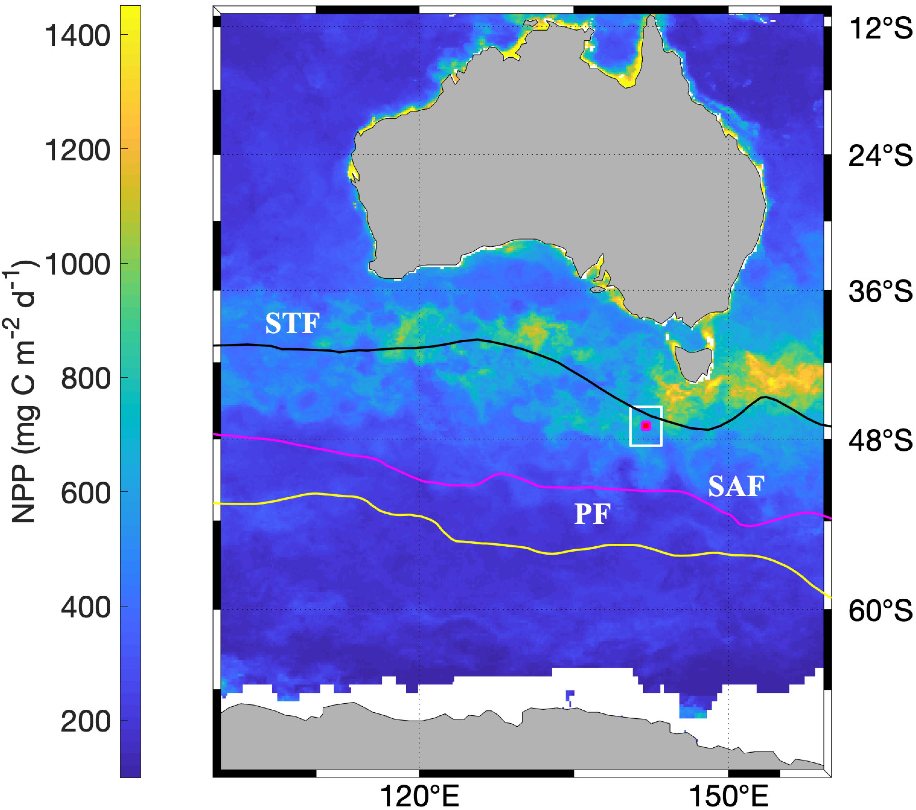
Figure 1. Location of the SOTS site (red dot) relative to average frontal positions (solid lines): Subtropical Front (STF), Subantarctic Front (SAF), Polar Front (PF). Background is Net Primary Production (illustrated for January 2012) as estimated from satellite remote sensing (see section “Materials and Methods”). The white square indicates the area used for NPP comparisons with SOTS particle fluxes.

Our goals in examining the long time series are:

1. to obtain a representative decadal estimate of the SAZ biological carbon pump (BCP),

2. to examine inter-annual variability in the BCP, including the possibility of a trend that might arise from anthropogenic impacts,

3. to characterize the seasonality of the total and component fluxes, as indicators of the probable environmental and ecological mechanisms that control the BCP strength in the Subantarctic Southern Ocean.

Materials and Methods

The Southern Ocean Time Series (SOTS) and Sample Collection

The Southern Ocean time series is a Sub-Facility of the Australian Integrated Marine Observing System (IMOS), which currently consists of two deep ocean moorings: the Southern Ocean Flux Station (SOFS) and the SAZ sediment trap mooring.

The SAZ moorings were deployed at ∼47°S, 140°E on the abyssal plain in the central SAZ in water depth of ∼4600 m. The sediment traps were McLane PARFLUX time-series conical sediment traps, with a 0.5 m² baffled funnel (2.5 cm baffle cell diameter) at the top and a carousel underneath that moved a series of cups under the funnel over the course of the deployment. The number of cups per trap and deployment varied between 13 and 21. Typically, the mooring was deployed with three sediment traps at nominal depths of 1000, 2000, and 3800 m except in years 2000 and 2005 (1000 and 2000 m) and 2003 (500, 1000, and 2000 m). For some of the deployments the controllers of the top two sediment traps contained tilt meters. In addition, the moorings were instrumented with current meters. Details of mooring designs, deployment voyages (and ancillary data such as CTD casts) are given in the SOTS Annual Reports (Wynn-Edwards et al., 2019). Long time series particle flux observations are particularly sparse for the Southern Ocean (but see Ducklow et al., 2008) and this time series covers nearly a full decade (from 2009–2017) and a partial decade in the late 1990s. The moorings were first deployed in September 1997 (Trull et al., 2001b) and maintained with some gaps until the present. With a few exceptions the moorings were deployed for 12 months, and trap cup sampling times ranged from 4 to 60 days. The time series has several data gaps (Figures 2A–C) due to sediment trap failures (deployment year 2005, partial data recovery), mooring loss (deployment years 2001, 2004, and 2006), vessel availability and insufficient trap sample material. The mooring was not deployed at 47°S in 2007, 2008, 2014, and 2017, owing to its use elsewhere, lack of ship time, or lack of funding. The 1000 m dataset for 2003/2004 was excluded due to suspected compromise of the mooring dynamics induced by the 500 m trap above.

FIGURE 2

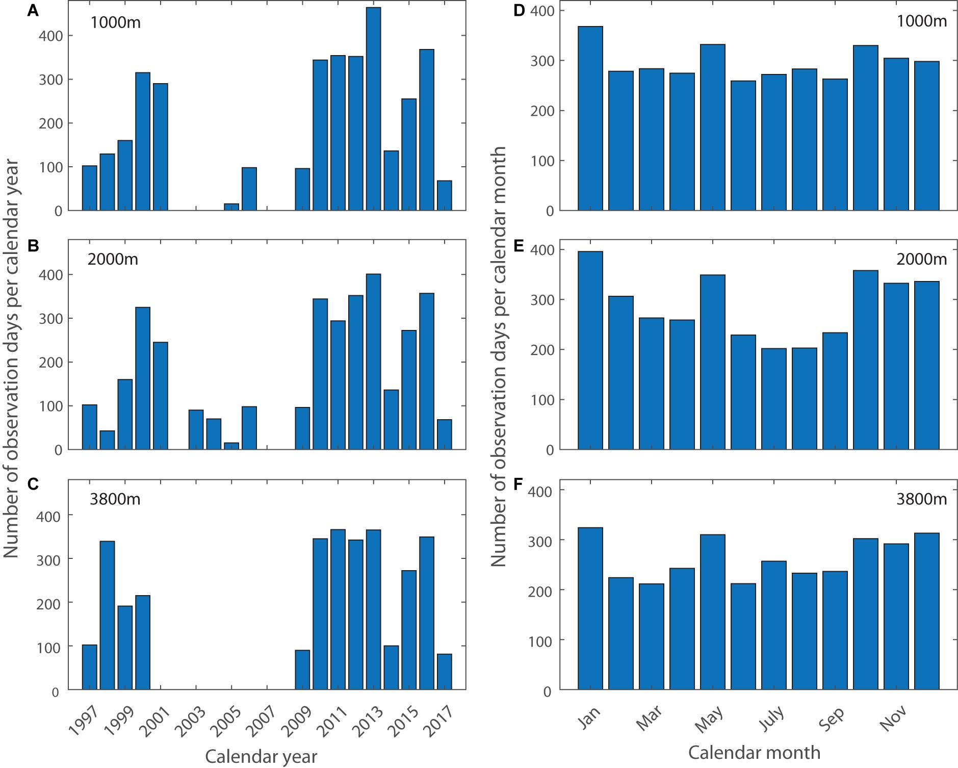
Figure 2. Statistics of 47°S sediment trap data per calendar year [(A) 1000 m, (B) 2000 m, (C) 3800 m] and month [(D) 1000 m, (E) 2000 m, (F) 3800 m]. During the calendar year 2013, two moorings were in the water at the same time for a short period, leading to observation days that exceed 365.

Assessment of the trap samples as a function of month of collection reveals a slight sample bias against winter, with highest sample numbers in austral summer in January across all three depths (Figures 2D–F).

Sediment Trap Preparation and Post Recovery Handling

Sediment trap cups were filled with a brine solution made up of 0.8 μm GF/F filtered seawater, collected close to the SOTS site. Typically, 5 g L^–1 NaCl was added to increase density and improve particle retention in the cups, as well as 2 g L^–1 Na₂B₄O₇ 10 H₂O to buffer pH and reduce carbonate dissolution, 0.22 g L^–1 SrCl₂ 6 H₂O for preservation of SrCO₄ acantharians and 3 g L^–1 HgCl₂ as a biocide.

After recovery of the mooring the sediment traps were hosed down with fresh water and allowed to settle for several days. Any unusual conditions, such as missing cups or trap failure (e.g., cups in position under the collection funnel on recovery) were recorded. Each cup had ∼20% of supernatant removed with a syringe via the fill hole to reduce the risk of spillage of poisoned brine on removing the cups from the trap carousel. The sample cups were then capped and stored refrigerated in the dark until transport to the onshore laboratory.

Sample Processing

The cups were allowed to settle for at least 3 days after transport to the onshore laboratory refrigerator. Samples were typically processed to dry matter within the following 2–3 months.

Photos of the cup collection were generally taken prior to any processing. The height of the solids in each cup was recorded after settling. Samples that had a noticeable foul odor or excessive organic material, e.g., large zooplankton (swimmers), were poisoned again with 100 μl of saturated mercuric chloride solution (HgCl₂). The sample cup supernatant was sampled for pH and salinity measurements and the remaining supernatant removed carefully and discarded. Particles in the cups were re-suspended and quantitatively transferred onto a 1 mm nylon sieve to remove swimmers. Where fecal pellets were present, they were photographed and rinsed through the sieve with a stream of buffered (1 g L^–1 Na₂B₄O₇ 10 H₂O), filtered seawater, followed by another photograph. The >1 mm fraction, mostly zooplankton, was stored in the buffered, filtered rinse seawater, re-poisoned if a foul odor indicated its necessity, and archived. The <1 mm fraction was split 10 ways using a McLane wet sample divider (McLane, WSD-10). Three splits were archived, and the remaining seven splits were re-combined, filtered onto 0.4 μm 47 mm polycarbonate membrane filters and dried over several days at 60°C to constant weight. The dried material was weighed and then scraped off the filter and homogenized by grinding to a powder using a mortar and pestle. Samples smaller than 10 mg dry matter were insufficient for further analysis and were left on their filters and archived. Quality assurance (QA) and assessment procedures, quality control (QC) tests and flagging decisions, as well as estimated measurement uncertainties are detailed in Wynn-Edwards et al. (2020).

Chemical Analyses

Only <1 mm dry material was analyzed for biogenic silica (BSi), PIC, particulate total carbon (PC), particulate total nitrogen (PN) and POC composition. Over the course of the programme, analytical methods have changed, and are described briefly here; for additional detail see Trull et al. (2001b) and the SOTS Annual Reports (Wynn-Edwards et al., 2019). From 1997 – 2000, total silicon was determined after digestion in HNO₃/HF closed Teflon bomb under heat and pressure in a digesting microwave oven, then analyzed by inductively coupled plasma/atomic emission spectroscopy (ICP-AES) (Bray et al., 2000). Between 2001 and 2013, BSi was determined by alkaline digestion and colorimetric analysis via segmented flow analysis (SFA) using an Alpkem model 3590 autoanalyser. Since 2015, BSi has been determined by the same alkaline digestion, followed by analysis at CSIRO’s hydrochemistry lab using similar segmented flow spectrometric methods (Rees et al., 2018). PIC was analyzed by conversion to CO₂ through addition of phosphoric acid, followed by coulometry, at the Woods Hole Oceanographic Institution, in the United States, between 1997 and 2000 and thereafter at CSIRO, in Australia. PC and PN were determined by combustion using a CHN Thermo Finnigan EA 1112 Series Flash Elemental Analyser at the Central Science Laboratory of the University of Tasmania. POC was calculated from PC by subtraction of PIC. No corrections were made for potential particle dissolution (Antia, 2005). Notably, these particle dissolution contributions can be significant, e.g., Trull et al. (2001b) estimated silica dissolution to represent 20–30% of the total silica flux and phosphate dissolution to range as widely as 10–80% with shallower traps usually around 20% and deep traps around 40%. No corrections were made for potential under- or over-collection during high tilt or current events, although ²³⁰Th observations from the 1997–1998 deployment suggested annual average under-collection of 30–40% was possible. The choice to make no corrections represents the uncertainties of these processes and their assessment, specifically that estimation of the dissolution component from the retained brine cannot assess the possibility of brine loss, and corrections based on radio-nuclide inventories are hampered by the likelihood that ²³⁰Th is associated with small surface-rich particles in contrast to the bulk components (mass, PIC, POC, BSi) which are delivered by large particles and accordingly correction was not recommended by the SCAR Working Group assembled report on trap methodologies (Buesseler et al., 2007a).

Data Processing

Mass and component flux data were evaluated and flagged according to Wynn-Edwards et al. (2020) and only data with QC flags 1 and 2 (good and probably good, respectively) were included in subsequent analyses. Across the deployment, cups were open for varying number of days, the midpoint date was used as the date of the cup result. Data gaps within deployments due to missing cup data were linearly interpolated from neighboring cups. The cup-by-cup data sets were then linearly interpolated on daily time steps for mass and component flux calculations per year. Due to the typical seasonality with peak particle flux in austral spring and summer (mid-September to mid-March, see Figure 7 and section “Possible Role of Seasonality in Control of Flux: Singular Value Decomposition”), and to avoid fragmenting these major flux events, the annual cycle was defined as 21st June to 20th June, rather than by calendar year. Daily interpolated data were only constructed for periods with data that covered a full annual cycle.

Data gaps between deployments were filled onto daily time steps via either of the following two ways, but only if the data gap fell outside of the main flux periods:

1. linear interpolation in six cases for the 1000 m, four cases for the 2000 m and six cases for the 3800 m data set; these gaps were no longer than 85 days;

2. extrapolation of the nearest data point to complete an annual cycle was used six times for the 1000 m, four times for the 2000 m, and five times for the 3800 m data set; these gaps were no longer than 117 days.

Based on cumulative annual flux calculations used in evaluating flux stability (see below) these duration gaps represent less than 10% of the average annual mass flux. If large data gaps fell within the main flux periods the data set was excluded for annual calculations.

In 2013, the deployment and recovery schedule resulted in two moorings sampling at the same time in close proximity. For the 1000 m traps there was an overlap between 26/05/2013 and 05/09/2013. Due to trap failure, the overlap was only one cup at 2000 m, between 26/05/2013 and 12/06/2013 and there was no overlap for the 3800 m traps. The overlapping mass and component flux results were averaged.

Results and Discussion

To address our goals as listed in the Introduction, we first present the average characteristics of the deep particle fluxes over the 20-year record and their attenuation with depth, and then examine their interannual, seasonal, and higher frequency variability. Our evaluation emphasizes potential controls on POC fluxes, including:

1. the influence of biogenic minerals, including the magnitude of the carbonate counter-pump,

2. the seasonal stability of the flux as an indication of possible decoupling of production and grazing,

3. the magnitude of surface productivity.

We begin with information gained directly from the flux measurements, and then compare to other observations.

Our analysis treats the observations as a time series of local processes in a 1-dimensional framework of settling particles, without explicit consideration of advective particle inputs from outside the region. We base this simplification on the location of SOTS within a small gyre lying between the eastward flowing Antarctic Circumpolar Current and westward flow to its north (Herraiz-Borreguero and Rintoul, 2011), low surface velocities estimated from satellite altimetry (∼20 cm s⁻¹ with occasional excursions to 50 cm s⁻¹ in mesoscale eddies Meijers et al., 2011), and currents as measured on the SOTS moorings (∼12 cm s⁻¹ with short excursions to <35 cm s⁻¹ at 1200 m, and decreasing further with depth; Bray et al., 2000 and the SOTS Annual Reports Wynn-Edwards et al., 2019 available on the AODN portal). These velocities suggest that most particles derive from sources close to SOTS. At 20 cm s^–1 (equivalent to 17 km d^–1) fast sinking particles (100 m d^–1) arrive at the 1000 m deep trap from no further than 170 km away. The source region to the deeper trap is only ∼50% larger, because current velocities decrease with depth. Moreover, as shown using a circulation model, the dominance of mesoscale eddies in the region confines the particle source regions to within a few degrees of latitude and longitude of the SOTS site for sinking rates greater than 30 m d^–1 (Hamilton, 2006). Further, this region is largely homogeneous in satellite ocean color images, and evaluation of statistical funnel effects (as described by Siegel et al., 1990) suggests local surface variations may add noise to seasonal records but do not bias their average seasonal cycle (Hamilton, 2006). While direct measurements of particle sinking rates are not available, gel trap analysis of sinking particles in the SAZ showed that most of the particles are large and therefore presumably fast sinking (Ebersbach et al., 2011). There are, however, some observations that suggest slowly sinking small particles may also influence the trap records. In particular, silicon isotopic variations suggest that slowly sinking small diatoms produced in summer do not arrive in the traps until winter (Closset et al., 2015), and study of suspended particles filtered from the top 600 m along a northward transect found rare earth element signatures suggesting inputs of small lithogenic clays from the Tasmanian shelf (Cardinal et al., 2001). Thus, while our 1-dimensional homogeneous source analysis seems appropriate for the major component fluxes, it comes with the caveat that allochthonous advective inputs may also occur, especially for small particles.

Average Particle Fluxes and Their Composition

The 20-year record of mass fluxes is shown in Figure 3, for both the cup-by-cup observed intervals and the interpolated daily resolution. The top three panels show the results for the first decade (Figures 3A–C), and the second three panels for the second decade (Figures 3D–F), during which higher data returns were achieved as the moorings became more durable and the deployment and recovery procedures more reliable. There is both considerable seasonal variability and interannual variability in the seasonality. Some summers have single peaks, others multiple events. Some winters have very low fluxes; others do not. Analysis of this variability is important to assess its causes and the associated implications for appropriate descriptions of ecosystem and export dynamics (as addressed in the sections below). As shown in Table 1, annual average fluxes (computed by breaking the records at 21st June each year to yield 7–9 years with full annual records, depending on the component and depth under consideration- see section “Materials and Methods”) are less variable, with a relative standard deviation of ∼45% at 1000 m depth, which tightens to ∼30% at 2000 m depth and less than 20% at 3800 m depth. This sense of relatively small interannual variability in the integrated annual fluxes (in contrast to strong seasonality and its interannual variability as mentioned above) implies that our determination of representative decadal average flux estimates (as listed in Table 1) is robust, but also requires the caveat that the full range of integrated annual flux values is quite large, decreasing with depth from ∼17-fold to 4-fold to 2-fold.

FIGURE 3

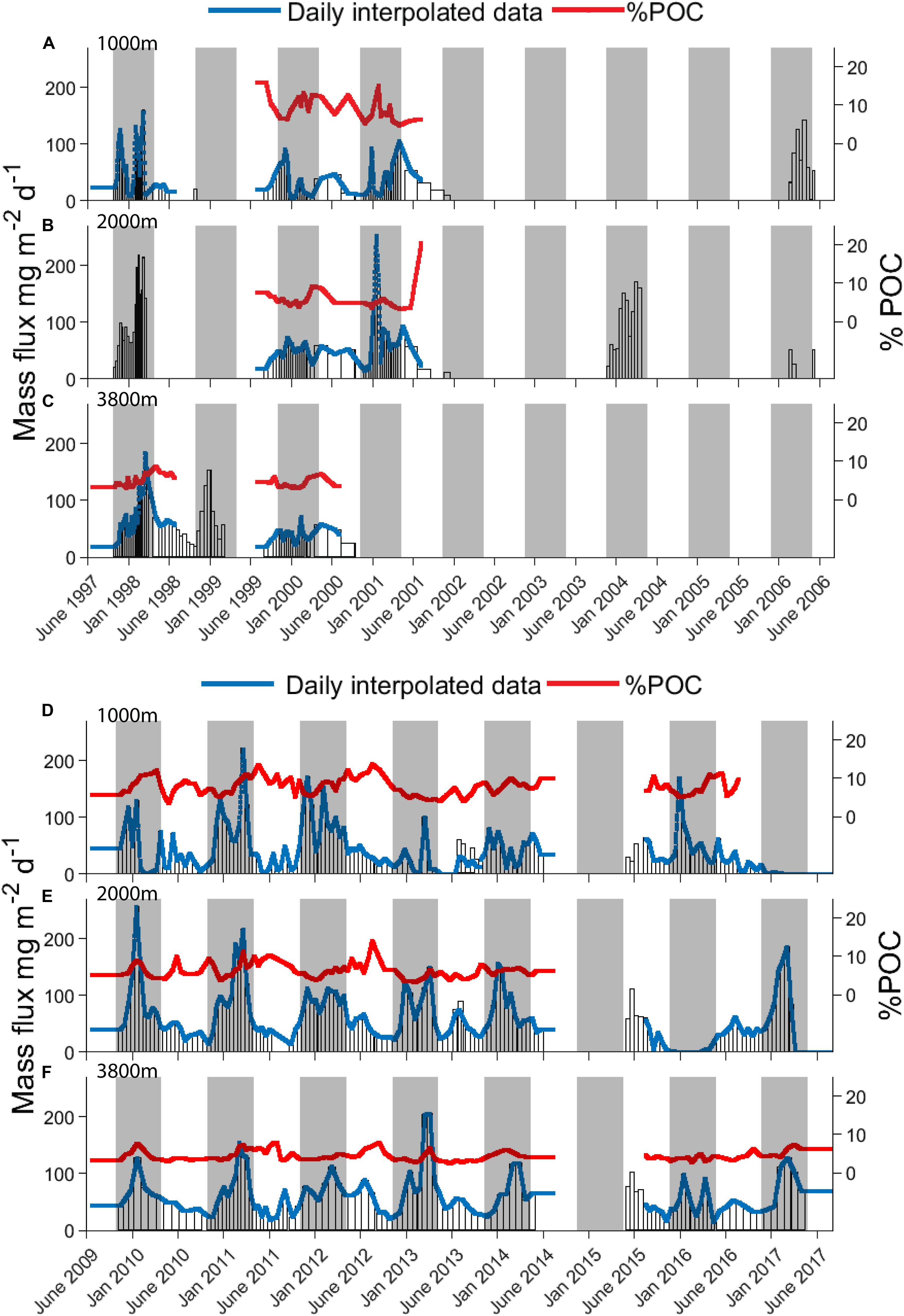
Figure 3. Multi-year record of mass fluxes at SOTS showing interannual variability in timing and amplitude of peak mass flux periods. Collection cup durations are represented by bar widths, with interpolated daily fluxes overlaid in blue and % POC (w/w) compositions in red. (A–C) Are for the first decade (June 1997 – June 2008) and (D–F) for the second decade (June 2008 to June 2017). Gray shaded areas represent the 6 months that cover the main flux period during early spring and summer, 21th September to 21th March, as shown by average fluxes discussed in section “Possible Role of Seasonality in Control of Flux: Mean Seasonal Cycles” and Figure 7.

TABLE 1

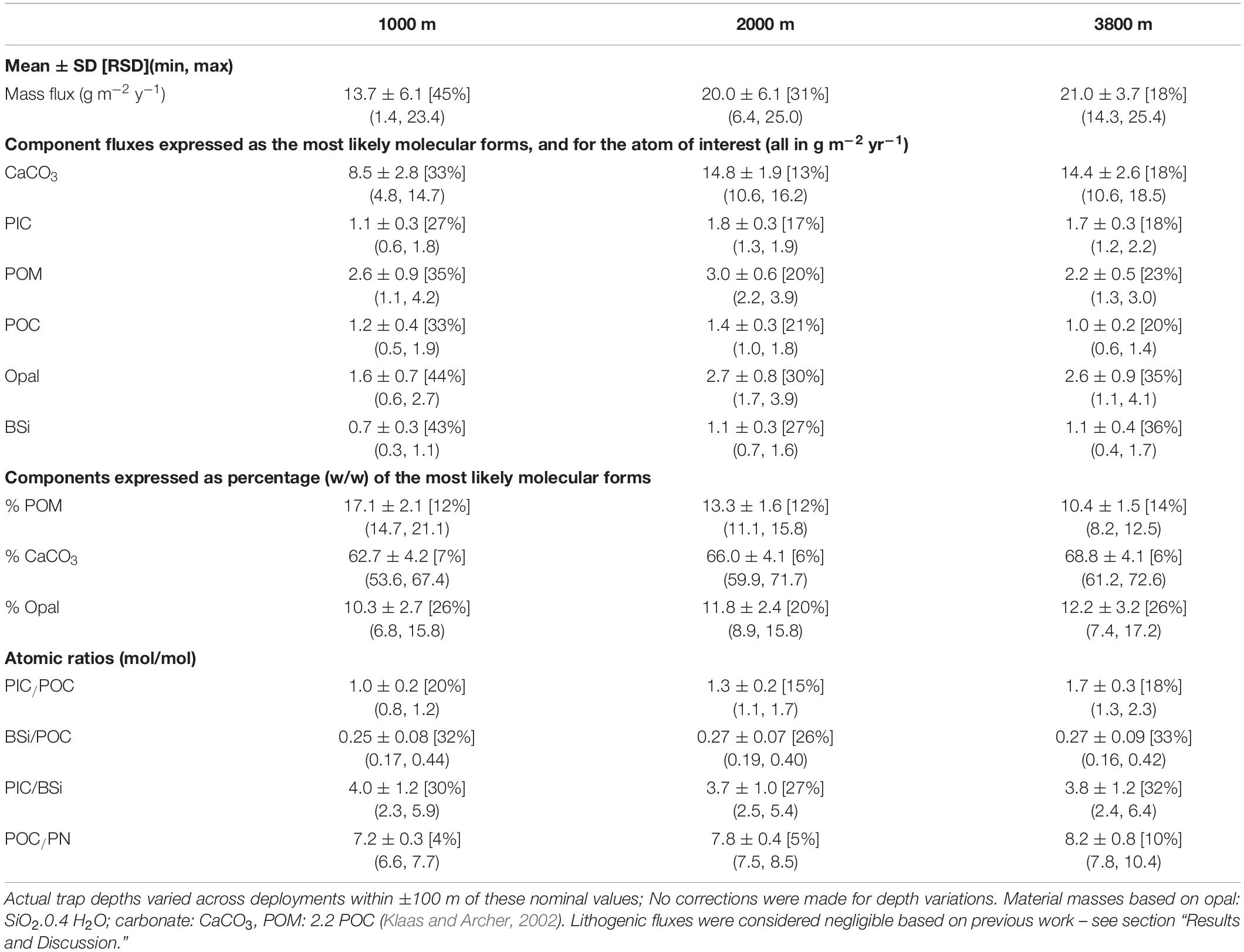
Table 1. SOTS average particle fluxes and compositions for the years with full records, minimum and maximum values in brackets, relative standard deviation expressed as percentage in square brackets.

The flux composition is more stable than its magnitude. This is seen readily by comparing the mass flux and %POC data in Figure 3, and by the average compositions in Table 1. The total mass flux at 1000 m depth is dominated by carbonate minerals (>60%), accompanied by opal (∼10%), and POM (∼17%). The contribution of POM decreases steadily with depth to ∼10% at 3800 m, with the other components showing smaller changes. Variability in the percent composition is small at all depths, well under 10% for the carbonate component, approximately twice this for POM, and slightly more for opal with the highest variability at 3800 m reaching 26%.

On a molar basis, inorganic carbon (PIC) is 4-fold more abundant than BSi and of similar abundance than organic carbon (POC) at 1000 m. Thus, the SOTS site is well-characterized as a “carbonate ocean” in the terminology of Honjo (Honjo et al., 2008), with secondary influence from biogenic opal, derived primarily from diatoms (Rigual-Hernández et al., 2015; Eriksen et al., 2018). The average POC flux of 1.4 ± 0.3 g m^–2 year^–1 at 2000 m is similar both to the first estimate made at the site in 1998 and to the global median (Trull et al., 2001b). Lithogenic fluxes have not been measured regularly, and previous work has suggested they are negligible (Trull et al., 2001b). However, the sum of the masses of the measured component fluxes is on average only ∼90% of the total measured mass fluxes, leaving open the possibility of lithogenic fluxes contributing up to 10% of the total flux. Comparing estimates of coccolithophore calcite (Rigual Hernández et al., 2019; Rigual-Hernández et al., 2020) and foraminifera shell weights (King and Howard, 2003; Moy et al., 2009) to total PIC fluxes suggests roughly equal contributions from these phytoplankton and zooplankton sources to the sediment trap collected carbonate fluxes (Trull et al., 2019). The POM had average POC/PN ratios that increased with depth (Table 1) and were above those expected for phytoplankton (Redfield, 1963; Copin-Montegut and Copin-Montegut, 1983), presumably as a result of preferential nitrogen remineralization (Honjo and Manganini, 1993; Conte et al., 2001; Schneider et al., 2003).

In summary, annual average fluxes at SOTS are close to the global median for POC, which is accompanied dominantly by PIC. Interannual variability is moderate (as represented by the standard deviations over 10 years for 1000 m and 9 years for 2000 and 3800 m). No long-term trends were present in any of the annual averages over the observational period (Figure 4 and additional analyses of the time series). The presence of PIC has important implications: it adds ballast to sinking aggregates which can enhance their delivery of POC to the ocean interior (Klaas and Archer, 2002). It also reduces the impact of the POC fluxes on the partitioning of CO₂ between the atmosphere and ocean, via the effect known as the carbonate counter-pump, in which each mole of carbonate precipitated increases seawater aqueous CO₂ by ∼0.6 mole (Frankignoulle and Gattuso, 1993), countering its removal by photosynthesis and the biological carbon pump. The importance of this counter-pump is usually assessed for the surface mixed layer, where the aqueous CO₂ content affects air-sea exchange, by assuming that deep trap PIC fluxes represent carbonate losses from the surface and back-extrapolating the deep trap POC fluxes to the mixed layer depth (e.g., Salter et al., 2014) assuming an attenuation function for the intervening depths, typically a canonical power law (Martin et al., 1987). That is, the effective carbon sequestration flux leaving the mixed layer can be written:

FIGURE 4

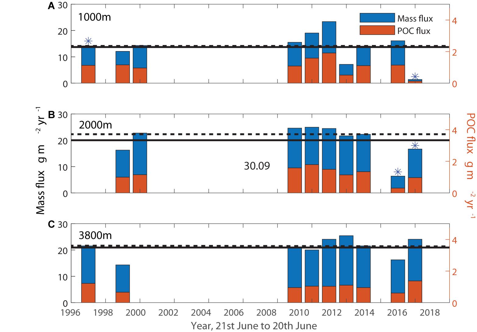
Figure 4. Annual mass and POC fluxes in g m^{– 2} yr^{– 1}. POC fluxes for years marked with * had gaps filled with average %POC values to complete an annual cycle for this figure. Median (dashed line) and average (solid line) mass fluxes do not include the years marked with *. (A) 1000 m, (B) 2000 m, (C) 3800 m.

$$Effective\mathrm{\_}Flux=Flux\mathrm{\_}POC\mathrm{\_}mld-0.6Flux\mathrm{\_}PIC\mathrm{\_}mld$$

with

$$Flux\mathrm{\_}PIC\mathrm{\_}mld=Flux\mathrm{\_}PIC\mathrm{\_}1000m$$

$$Flux\mathrm{\_}POC\mathrm{\_}mld=Flux\mathrm{\_}POC\mathrm{\_}1000m(mld/1000){}^{-}{}^b$$

Using 100 m for the summer mixed layer depth when production is significant (Trull et al., 2019), b = 0.858 (Martin et al., 1987), and the average PIC/POC at 1000 m of 1.0 ± 0.2 (Table 1) suggests the presence of PIC reduces the effectiveness of the biological organic carbon pump by 8 ± 2%. This is similar to previous Southern Ocean estimates (Salter et al., 2014). Clearly this efficiency estimate is approximate and dependent on many assumptions. Notably, the attenuation of POC flux with depth at SOTS may be higher than expected from the Martin et al. (1987) formulation, as discussed in the next section, and this would reduce the impact of the carbonate counter-pump on carbon sequestration.

Finally, the importance of PIC at SOTS implies that the ecosystem and its biological pump are likely to be susceptible to ocean acidification. In this regard, previous work has suggested that foraminifera shell weights at SOTS are lower than during the pre-industrial Holocene, by amounts consistent with expectations from ocean acidification (Moy et al., 2009). In contrast, study of recent decadal variations in pteropod fluxes at SOTS showed both increases and decreases over time, depending on the species examined (Roberts et al., 2014). Carbonate mineral saturation states are currently still relatively high in the SAZ (Trull et al., 2018), but are expected to diminish strongly by the end of the century at which time impacts may increase (Orr et al., 2005), and the present SOTS observations provide a well determined baseline and an archived set of samples for later comparisons.

Flux Variations With Depth: Observations

On average sediment traps at 1000 m recorded a lower mass flux than the two deeper traps. This apparent under-collection has been reported previously (Honjo and Manganini, 1993; Yu et al., 2001; Berelson, 2002) and tentatively attributed to a combination of stronger currents at shallower depths that reduce trapping efficiency and mesopelagic processes that lead to increased compacting and aggregation of sinking particles below 1000 m which lead to improved trapping efficiency at greater depth. Since there is currently no consensus on the magnitude that currents and tilt might have on trapping efficiency (Gardner, 1985; Buesseler et al., 2007a), we did not correct our flux data (see section “Materials and Methods”).

The range of mass fluxes was largest at 1000 m and decreased with depth. Interestingly, the largest fluxes measured at all three depths over the time series were similar, while the smallest fluxes which occurred at 3800 m were vastly greater than those at 1000 and 2000 m. The highest cup flux measured was 222 mg m^–2 d^–1 at 1000 m, 256 mg m^–2 d^–1 at 2000 m and 205 mg m^–2 d^–1 at 3800 m. The lowest cup mass flux measured at 1000 m was 0.2 mg m^–2 d^–1 and 0.1 mg m^–2 d^–1 at 2000 m but never less than 13.9 mg m^–2 d^–1 at 3800 m. POC fluxes at SOTS ranged between 4 and 2298 mg m^–2 d^–1 at 1000 m, 67 and 2457 mg m^–2 d^–1 at 2000 m and 54 and 1312 mg m^–2 d^–1, which may seem large but is in line with other time series and smaller than that reported for the upper 500 m at the BATS time series station at 32°N, 64°W (0.1–311 mg POC m-2 d-1 between 1998 and 2016, Johnson and Pacheco, 1998-2016)¹. The average attenuation of POC flux in g m^–2 d^–1 from 2000 to 3800 m was 29%, similar to previously reported attenuations between 1500 and 3200 m of 25% in the western Sargasso Sea (Conte et al., 2001).

As noted in the previous section, the standard deviation of annual mass fluxes decreased with depth. This was broadly speaking also true for POC, with relative standard deviations of 35, 21, and 24% at 1000, 2000, and 3800 m, respectively. Decreases in the variability of BSi and PIC fluxes with depth were smaller (Table 1). Overall, the compositional information is consistent with the view that flux composition becomes more homogeneous with depth, either as a result of removal of labile components from all particles (Conte et al., 2001), or the ability of only a limited class of particles to reach the deep sea (Boyd and Trull, 2007; Trull et al., 2008). Reduced flux variability could also be due to the increased spatial and temporal statistical funnel at greater depth (Siegel et al., 1990). The statistical funnel refers to the theoretical surface area from which particles most likely originated, which depends on the particle sinking speed and the three-dimensional fluid velocity acting on the particle as it sinks.

Flux Variations With Depth: Comparisons to Common Algorithms

The most commonly used algorithm for C export attenuation is the empirical formulation of Martin et al. (1987)

$$C_{flux\left(z\right)}=C_{export}{\left(\frac{z}{z_0}\right)}^{-0.858}$$

where C_flux(z) represents carbon flux at depth z and C_export the carbon exported from the surface ocean at depth z_o, typically taken as the mixed layer depth. C_export is equivalent to net community production (NCP) in a steady-state system (assuming negligible DOC export). NCP at the SOTS site has been estimated using a range of techniques: mixed layer O₂/N₂ budgets (Weeding and Trull, 2014), nitrogen depletion in the surface layer (Lourey and Trull, 2001), ²³⁴Th surface water deficit measurements (Jacquet et al., 2011) and a dissolved inorganic carbon budget (Shadwick et al., 2015), and reported values range from 3 to 6 mol C m^–2 yr^–1. POC fluxes at the SOTS site thus represent 2–3% of NCP at 1000 m, 2–4% at 2000 m and 1–3% at 3800 m. In comparison, using z₀ of 100 m and the b value of −0.858 proposed by Martin et al. (1987) based on limited observations from the Pacific Ocean, ∼8% of NCP would arrive at 2000 m. A wide range of b values from 0.5 to 2 have been shown to occur globally (Boyd and Trull, 2007 and ref. therein), in which case 0.3 – 22% of NCP can be expected to arrive at 2000 m, and the POC fluxes at 2000 m over the 20-year time series place the b value at 1.1 to 1.3 for z₀ 100 m, i.e., higher than the canonical Martin b value but well within the global range of power-law attenuation coefficients.

An earlier algorithm for POC flux at depth related it directly to Net Primary Production (NPP) (Suess, 1980)

$$C_{flux(z)}=C_{NPP}\mathrm{/}(0.0283z+0.212)$$

where C_flux(z) represents carbon flux at depth z and C_NPP is the rate of NPP in carbon units. The dependence on depth is equivalent to a power law b value of 1, and thus the attenuation is similar; while the expression in terms of NPP convolves the attenuation with depth with the fraction of NPP that escapes the surface layer, commonly described by the e-ratio, and taken as equivalent to the fraction of new production known as the f-ratio over the annual mean (see Boyd and Trull, 2007 for discussion).

Satellite ocean color-based estimates using the VGPM algorithm (see section “Possible Role of Net Primary Production in Control of Flux” for details) place the average annual NPP between 2009 and 2016 at 138 ± 14 g C m^–2 yr^–1 at SOTS. There are several sources of potential bias in this estimate of NPP in the Southern Ocean, including that phytoplankton chlorophyll-a is likely underestimated by standard ocean color algorithms (e.g., Johnson et al., 2013) and large variations among productivity models have been reported (e.g., Carr et al., 2006). Putting those caveats aside, comparing the SOTS sediment trap POC fluxes to this annual NPP estimate suggests ∼0.8 ± 0.4% of surface NPP arrives at 1000 m depth (0.9 ± 0.4% at 2000 m and 0.7 ± 0.2% at 3800 m), which is less than half of the 1.8% expected from the Suess algorithm.

The SOTS trap-based fluxes at 2000 m of 2–4% of NCP are also low compared to estimates of ∼15% from Weber et al. (2016) and DeVries and Weber (2017) based on large-scale ocean nutrient distributions, and the estimate of <5% from Henson et al. (2012) for the Southern Ocean (euphotic zone to 2000 m) based on satellite productivity and ²³⁴Th measurements. In summary, POC transfer efficiency at SOTS seems to be lower than expected from commonly used export models but within the ranges of values observed globally and elsewhere within the Southern Ocean (Boyd and Trull, 2007; Buesseler et al., 2007b; Maiti et al., 2013).

Can We Explain the Interannual Variability of Mass or POC Fluxes?

Broadly speaking, interannual flux variability should derive from differences in surface primary productivity (stage 1), the component of this production exported from surface waters (stage 2), and/or attenuation at mesopelagic depths (stage 3), with each of these stages considered to contribute similarly to flux variations at global scale (Boyd and Trull, 2007). Previous conceptions of important controls on these processes have included the ballast hypothesis (Armstrong et al., 2001) in which the presence of biogenic minerals increases sinking rates and reduces remineralization rates thereby enabling more POC to reach the deep sea (influencing stage 3), and the flux-stability hypothesis (Lampitt and Antia, 1997) in which systems with strong seasonality are considered to achieve decoupling of production and grazing thereby enabling greater export (influencing stage 2). We investigate each stage of the BCP by considering the mechanisms that influence the three stages outlined above. The influence of stages 3 and 2 can be gauged using our time series observations, and the possible role of stage 1, primary production, by comparison to satellite-derived productivity estimates. We first examine the role of ballast (see section “Possible Role of Particle Ballast in POC Flux Magnitude”) and then seasonality via the flux stability metric [see section “Possible Role of Seasonality in Control of Flux – The Flux Stability Index (FSI)”], mean seasonal cycles (see section “Possible Role of Seasonality in Control of Flux: Mean Seasonal Cycles”), and SVD to derive seasonal modes (see section “Possible Role of Seasonality in Control of Flux: Singular Value Decomposition”). Finally, we compare the annual mean fluxes to annual mean NPP (see section “Possible Role of Net Primary Production in Control of Flux”).

Possible Role of Particle Ballast in POC Flux Magnitude

The importance of ballast minerals for POC flux to depth has been widely explored, and there is a growing understanding that the magnitude of POC export from the surface might be less important than the composition of the particles and site specific mesopelagic processes (Buesseler et al., 2007b). Independent of the magnitude of NPP, how particles sink and what happens to them on the way down, i.e., attenuation mechanisms, play an important role in determining the magnitude of flux at depth. Flux attenuation is a function of sinking velocity and how well the particles can be remineralized or how likely they are to be grazed on their path down. It has been proposed that plankton community structure influences both the exported fraction (i.e., the f-ratio) and the flux attenuation mechanisms. A NPP with a high percentage of diatoms may to lead to high export ratios but low transfer efficiency due to the labile state of the POC associated with diatom-dominated particle export (Lima et al., 2014). Conversely, particle fluxes dominated by calcifiers can have a higher transfer efficiency, due to faster sinking velocities and reduced particle porosity (Guidi et al., 2009; Lima et al., 2014; Bach et al., 2016, 2019; Mouw et al., 2016), although Honda and Watanabe (2010) found a higher POC carrying capacity for BSi than PIC in the sub-arctic northwest Pacific.

At SOTS, the annual POC flux was positively correlated with PIC flux only at 1000 m (adjusted R² = 0.8, p = 0.0009), and not at the two depths below (p > 0.1) whereas annual POC fluxes were positively correlated with annual BSi fluxes at all three depths (adjusted R² = 0.7, p = 0.006, adjusted R² = 0.8, p = 0.004 and adjusted R² = 0.8, p = 0.0006 for 1000–3800 m, respectively). This could indicate that the presence of diatoms increases POC transfer to depth in the Subantarctic, as found in the sub-arctic (Honda and Watanabe, 2010). Expressing the particle composition as a ratio of the two ballasting components (PIC and BSi, Figure 5A), also shows that on an annual basis lower PIC/BSi molar composition of sinking particles is weakly associated with higher POC fluxes (1000 m adjusted R² = 0.5, p = 0.04; 2000 m adjusted R² = 0.6, p = 0.03; 3800 m adjusted R² = 0.5, p = 0.03), challenging the notion that diatom-dominated POC export is more labile and therefore has a lower transfer efficiency (Lima et al., 2014). The correlation between PIC/BSi molar ratio and transfer efficiency (expressed as the percentage of NPP carbon arriving at depth) is much weaker and only statistically significant at 1000 m (adjusted R² = 0.9, p = 0.004, 2000 m p = 0.2 and 3800 m p = 0.06, Figure 5B). This is consistent with the finding in section “Possible Role of Net Primary Production in Control of Flux” below that annual POC fluxes were independent of NPP. The molar ratio of PIC to BSi was also not correlated with annual NPP (Figure 5C). In combination, these observations suggest that biogeochemically defined phytoplankton functional types (diatoms, coccolithophores) influence either the fraction of NPP that is exported, or its subsequent attenuation (or both together) as it transits the mesopelagic zone, while the magnitude of NPP is not a useful predictor for POC fluxes beyond 1000 m.

FIGURE 5

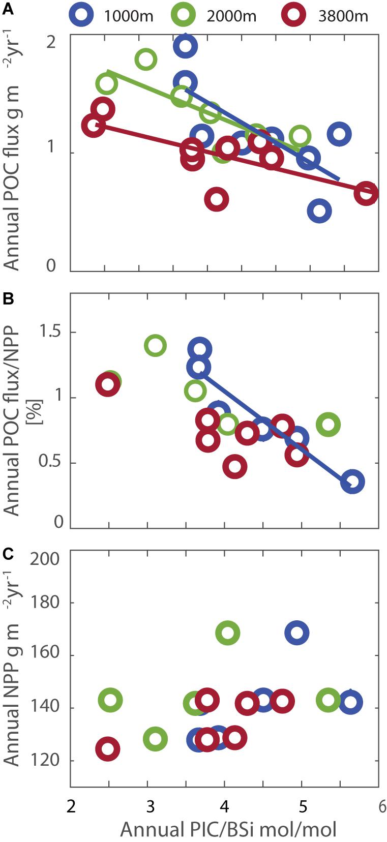
Figure 5. Relationships between the two major ballasting components of sinking particles (expressed as their ratio PIC/BSi on the x-axes) and POC flux (A), NPP (B), and the transfer efficiency (expressed as POC flux/NPP, C). Trend lines are shown only for statistically significant correlations.

Possible Role of Seasonality in Control of Flux – The Flux Stability Index (FSI)

A conventional view (e.g., Lampitt and Antia, 1997) of particulate fluxes is that large annual mass fluxes are the result of short-duration, but large magnitude events (in high latitude and temperate systems), while smaller annual fluxes are the result of smaller magnitude events occurring consistently through the year (in tropical/oligotrophic systems). To quantitatively distinguish between these two flux behaviors, Lampitt and Antia (1997) devised the Flux Stability Index (FSI), in which measured fluxes are sorted by decreasing magnitude, irrespective of their seasonal timing, and the FSI is given by the number of days required to accumulate 50% of the annual flux.

The average FSI computed at each trap depth (Figure 6) were not statistically different from each other and ranged from 87 ± 21 days at 1000 m, to 98 ± 28 at 2000 m, to 120 ± 19 at 3800 m. These values are at the higher end of the global range reported by Lampitt and Antia (1997), and accordingly relatively low annual POC fluxes would be anticipated. However, as noted in section “Average Particle Fluxes and Their Composition,” the SOTS POC fluxes are close to the global median. The FSI values at the site varied interannually over much of the global range, but there was no statistically significant correlation between FSI and annual POC fluxes (Figure 6A), nor between the FSI and the transfer efficiency expressed as percentage of NPP arriving at depth (Figure 6B). This lack of significant relationship between FSI and mass flux was also observed by Lampitt and Antia (1997) for polar regions and may be due to significant fluxes during non-peak seasons, which have also been observed at SOTS (Figure 3). A closer look at the seasonality at SOTS is provided in the next section.

FIGURE 6

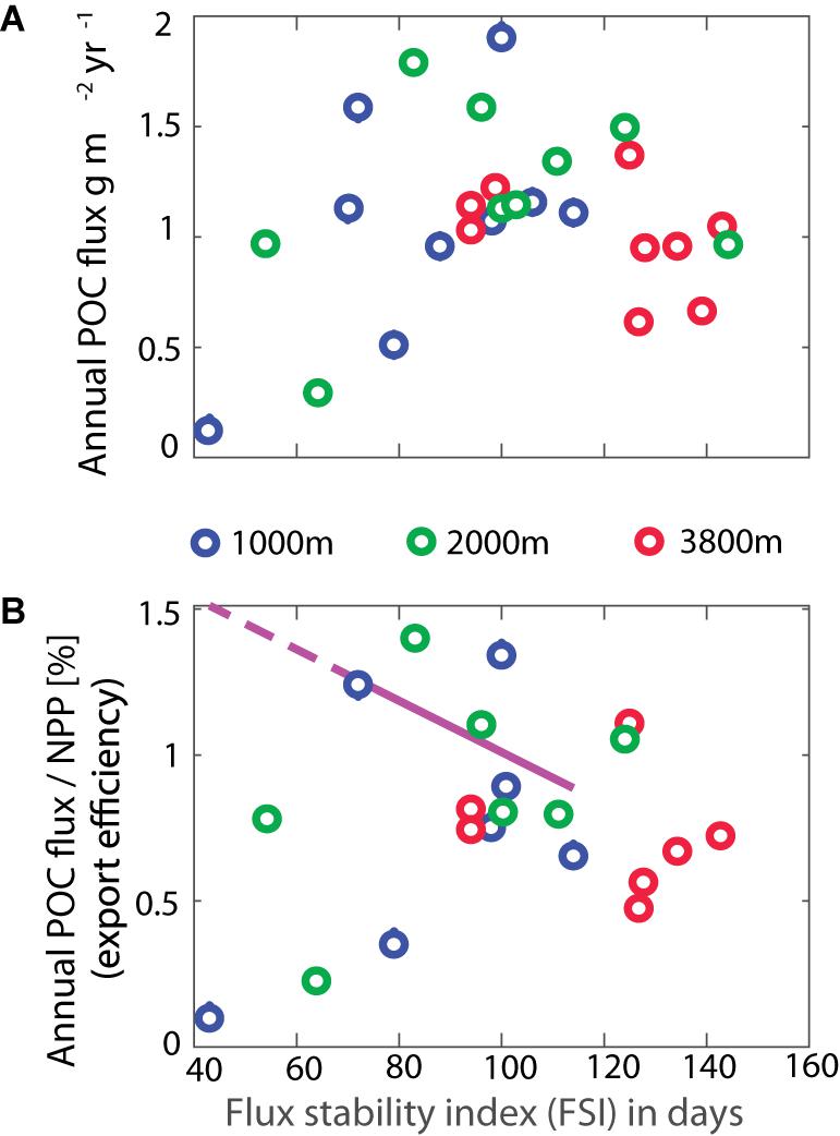
Figure 6. Comparisons of POC flux (A) and transfer efficiency (B) with the flux stability index (FSI) revealed no significant correlations. The pink dashed line shows the relationship between transfer efficiency and FSI proposed for non-polar regions by Lampitt and Antia (1997).

FIGURE 7

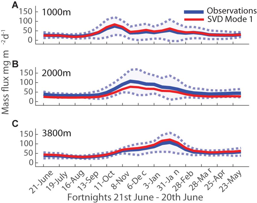
Figure 7. Mass flux seasonality at each depth: (A) 1000 m, (B) 2000 m, (C) 3800 m. Fortnightly averages in blue, with blue shaded area representing 1 SD. The first mode from the SVD analysis is shown in red.

Possible Role of Seasonality in Control of Flux: Mean Seasonal Cycles

Given that annual POC flux is correlated with particle composition, and thus likely with ecosystem structure, a closer look at flux seasonality might help shed some light on the source of this correlation. This is also motivated by the long-standing recognition that organic matter available from the euphotic zone arises from the small imbalance between autotrophic production and its heterotrophic consumption, and this imbalance may be larger when there is strong seasonality owing to the generally longer life cycles of heterotrophs (e.g., Evans and Parslow, 1985; Morel et al., 1991; Lutz et al., 2007; Lindemann and St John, 2014). To construct a mean flux seasonality, daily interpolated mass flux data was averaged over fortnightly intervals (Figure 7, blue line, shaded area). The resulting mean seasonal cycle is best described by a temperate, early spring and late summer, two-peak pattern at all three depths. This is most clearly distinct at 1000 m, with the peaks overlapping at 2000 and 3800 m (where their distinct nature is mainly discernible via the compositional variations (Figure 8). Variability during peak flux periods is reduced with depth, as seen in the reduced standard deviation envelope around the mean flux in Figure 7. The largest standard deviation falls into the summer period of December and January, indicating that the timing and magnitude of the summer flux peak is variable across years. Looking at individual years (Figure 3), the large standard deviation for the 1000 m flux data in January is due to the varying timing of the secondary peak (Figure 7A). At 2000 m, the standard deviation of the mass flux data in December is large since half of the analyzed years had no peak flux in December (Figure 7B). Explanations for the change in seasonal pattern with depth include a time shift in the observed peak flux from October to January moving from 1000 to 3800 m due to slow sinking particles, and the possibility that the late summer peak at 1000 m does not penetrate to depth. It is also possible to view the background flux at 3800 m during winter as a result of slow sinking particles originating from the late summer peak at 1000 m (Closset et al., 2015). Fluxes during winter at 3800 m never reach zero and are far greater than those measured at 1000 and 2000 m during the same period (as stated in section “Flux Variations With Depth: Observations”). An alternative explanation could be that particles from the spring peak at 1000 m are attenuated more quickly, and this explains the near absence of the first peak at 3800 m – in this view the main peak at 3800 m would be derived from the late summer peak observed at 1000 m, via very rapid particle sinking (Conte et al., 2001). Cross-covariance calculations with daily interpolated mass flux data (as described by Conte et al., 2001) and with component ratios of particles across depth (modified after Berelson, 2002) indicated that particle sinking speeds are in the order of days, i.e., hundreds of meters per day (data not shown).

FIGURE 8

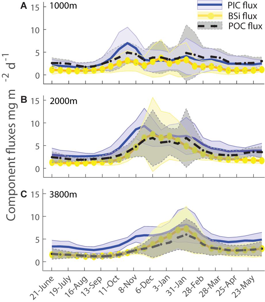
Figure 8. Seasonal component flux variations at each depth: (A) 1000 m, (B) 2000 m, (C) 3800 m. Lines show average values; shaded envelopes show 1 SD.

Figure 8 shows the seasonal variations in the component fluxes of PIC, POC, and BSi, which deviate slightly from the pattern of mass fluxes. The PIC flux has a similar two-peak shape at all three depths, with the same shape and timing as total mass flux, unsurprising due to its dominant role in particle composition. The BSi flux at 1000 m appears more diffuse across a broad time frame, from spring to summer (October to February), with three possible minor peak flux events. This is in line with diatom fluxes found in sediment trap material from 1999–2001 (Rigual-Hernández et al., 2015). At 2000 and 3800 m biogenic silica flux was similar to that of the mass flux in its overlapping two peak seasonality. The concept of multiple episodes of BSi export is consistent with seasonal surface phytoplankton community observations via autonomous water sample collection during the 2010/2011 deployment, which indicated that diatom biovolume peaked in late September, with contributions from large diatoms highest in early December, and the late summer community exhibiting more weakly silicified frustules (Eriksen et al., 2018). The average POC flux was highest in the spring to summer period, again with three possible peak flux events at 1000 m, two peaks at 2000 m and two overlapping peaks at 3800 m. Average POC fluxes were largest in late January, when interannual standard deviations were also largest.

Possible Role of Seasonality in Control of Flux: Singular Value Decomposition

Calculating average fortnightly total mass and component fluxes and their associated standard deviations helps to describe the mean seasonality and how much it varies between years, but is in itself not an explanation for the interannual variability in mass or POC flux. To help us quantify whether the seasonality of fluxes and its variability influences total annual POC flux we used the results of a Singular Value Decomposition (SVD) as explained in the next section.

SVD offers an objective way to elucidate underlying patterns in time series, via least-squares minimization to deconvolve them into a reduced set of orthogonal modes that are ranked in order of the fraction of variance they explain (e.g., Cadzow et al., 1983; Yoder and Kennelly, 2003; Kim et al., 2016; Trinh and Ducklow, 2018). To do this, our time series was divided into annual cycles (at 21st June of each year, see section “Materials and Methods”) with fortnightly resolution, providing 10 records for 1000 m, and 9 records for the deeper depths (2000 and 3800 m). The first 3 modes captured nearly all the variance (at all depths), and we focus our discussion accordingly. The first mode of the SVD analysis is overlaid on the fortnightly mass flux averages in Figure 7 (red line), and has very similar seasonality to the average fluxes, i.e., it exhibits spring and late summer peaks. It explained 79% of the variability in mass fluxes at 1000 m, 85% at 2000 m and 93% at 3800 m.

The first three modes for the 1000 m mass fluxes are compared in Figure 9A. Mode 1 describes the dominant temperate seasonal pattern of a spring bloom (in October) and secondary late summer (late January) peak. Mode 2 shows that a relatively strong summer peak is associated with a late start to the spring peak (and vice versa). Mode 3 indicates that a short duration spring peak is associated with an early and short duration secondary peak (and vice versa). Modes 2 and 3 each explain similarly small portions of interannual variance of 8 and 5%, respectively. The majority of interannual variation in mass fluxes is therefore explained by a typical seasonality (Mode 1) with varying contributions to the flux magnitudes each year, as shown by seasonal representation of Mode 1 for the 10 years at 1000 m in Figure 10A, i.e., high and low flux years therefore share a common seasonality of two peaks. Figures 9B, 10 also show that Modes 2 and 3 vary in their sign across the time series, and that there is no overall trend in any of the three Modes. While Mode 1 dominates the other two modes, individual years stand out, e.g., in 2010 when the influence of Mode 2 is similar to Mode 1 in other years (Figure 10B). Despite this variation in the strength of Mode 2 and 3 for individual years, their annual coefficients do not correlate with annual mass flux (not shown) and so the timing of total mass peak flux events does not explain interannual variability in total mass flux. This has important ramifications for the evaluation of ecological hypotheses based on decoupling of production and grazing in the control of POC fluxes, as discussed below.

FIGURE 9

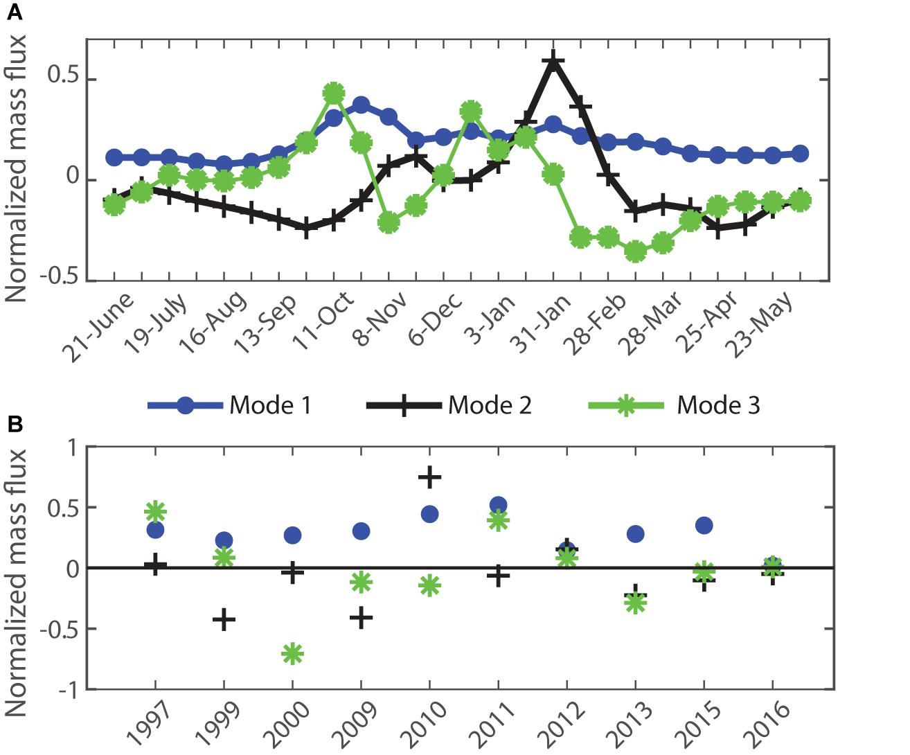
Figure 9. Singular Value Decomposition for mass flux at 1000 m (A) Seasonal structure of Modes 1 – 3. (B) Interannual time series of the principal component coefficients of Modes 1–3. The % variance explained by these Modes was 79, 8, and 5%, respectively.

FIGURE 10

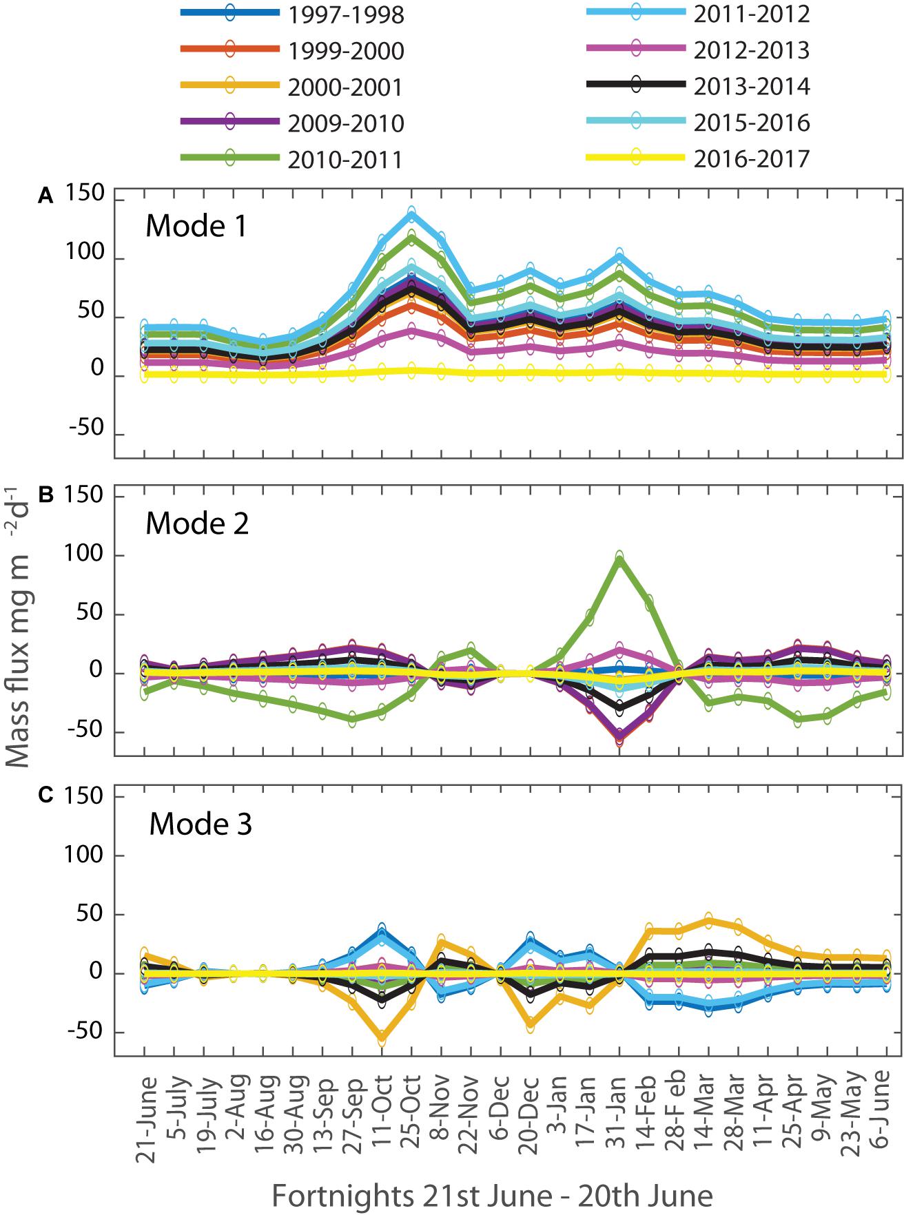
Figure 10. Interannual variations in the seasonal 1000 m mass flux contributions of the Singular Value Decomposition Modes. (A) Mode 1: 79%, (B) Mode 2: 8%, (C) Mode 3: 5%.

Mode 1 for mass fluxes at 2000 and 3800 m explains an even larger percentage of the interannual variances, 85 and 93%, respectively. Again, most of the interannual variation in mass fluxes is explained by the differences in Mode 1 mass flux magnitudes and to a lesser extent by the timing of the peak flux events. The seasonality of mass fluxes at 2000 m is best described by a broad, possibly overlapping double-peak in late November (Figure 7B). At 2000 m, Mode 2 explains more than twice as much of the interannual variability than Mode 3 (7 and 3%, respectively). Mode 2 represents a change in the timing of the peak flux events at 2000 m by a few weeks from year to year and Mode 3 shows that for years with smaller fluxes during summer, mass fluxes occur later in the year and vice versa (data not shown). The seasonality of mass fluxes at 3800 m is also best described by an overlapping double peak, however, much later than at 2000 m, in late January (Figure 7C). Mode 2 explains 4% of the variability and with only 1% Mode 3 is not considered further here. Mode 2 indicates that years with relatively small peak mass flux in January exhibit increased mass fluxes throughout the rest of the year (1997/1998, 2010/2011, and 2012/2013, data not shown). The larger statistical funnel for particle collection at 3800 m depth likely explains the high percentage of variability accounted for by Mode 1. This deepest trap collects particles over a larger spatial range and slow sinking particles originating in high flux periods during summer can arrive at greater depths during later low flux periods, smoothing out the seasonal variation at greater depth (Closset et al., 2015).

In summary, variations in the timing of peak flux events (characterized by Modes 2 and 3) explain a small proportion of interannual flux variability and as such do not help to explain interannual variability in total flux. That variability is dominated by the changing intensity of Mode 1. Analysis of the time series of mode coefficients did not reveal any trends, and thus there is not yet evidence of change in the spring initiation of productivity or the duration of the production season, as expected from century timescale coupled climate change and ocean biogeochemistry simulations (e.g., Bopp et al., 2001; Gehlen et al., 2006; but see Ducklow et al., 2008).

This analysis of the role of seasonality in interannual flux variations has been built on the Modes of mass flux. It is possible to also estimate Modes for each major component (PIC, BSi and POC) separately (as shown in Figure 11 for 1000 m depth). Again, the first Mode explains most of the variance of each of the flux constituents. For PIC Mode 1 has a very similar shape to that of mass flux, with somewhat greater influence of the first spring peak relative to the summer peak. BSi Mode 1 exhibits an intervening December peak, and thus less distinct separation into two separate flux events. POC Mode 1 combines aspects from both of these other components, with spring and especially summer peaks and a smaller intervening flux component. This explains 78% of interannual variability. The difference in timing of component peaks, with the PIC in late October and the BSi in late December, in comparison to peak POC fluxes in late January, seem to place more emphasis on opal forming plankton as POC carriers. Seasonally varying processes in the mesopelagic that might lead to stronger POC flux attenuation in spring versus late summer, however, cannot be ruled out. Modes 2 and 3 of component fluxes at all three depths do not correlate with annual POC flux, again indicating that the timing of peak flux events, whether it be total or that of any particular component, does not explain interannual variability of POC flux. There was also no temporal trend in the coefficients of Modes 1–3 for the components at any of the three depths.

FIGURE 11

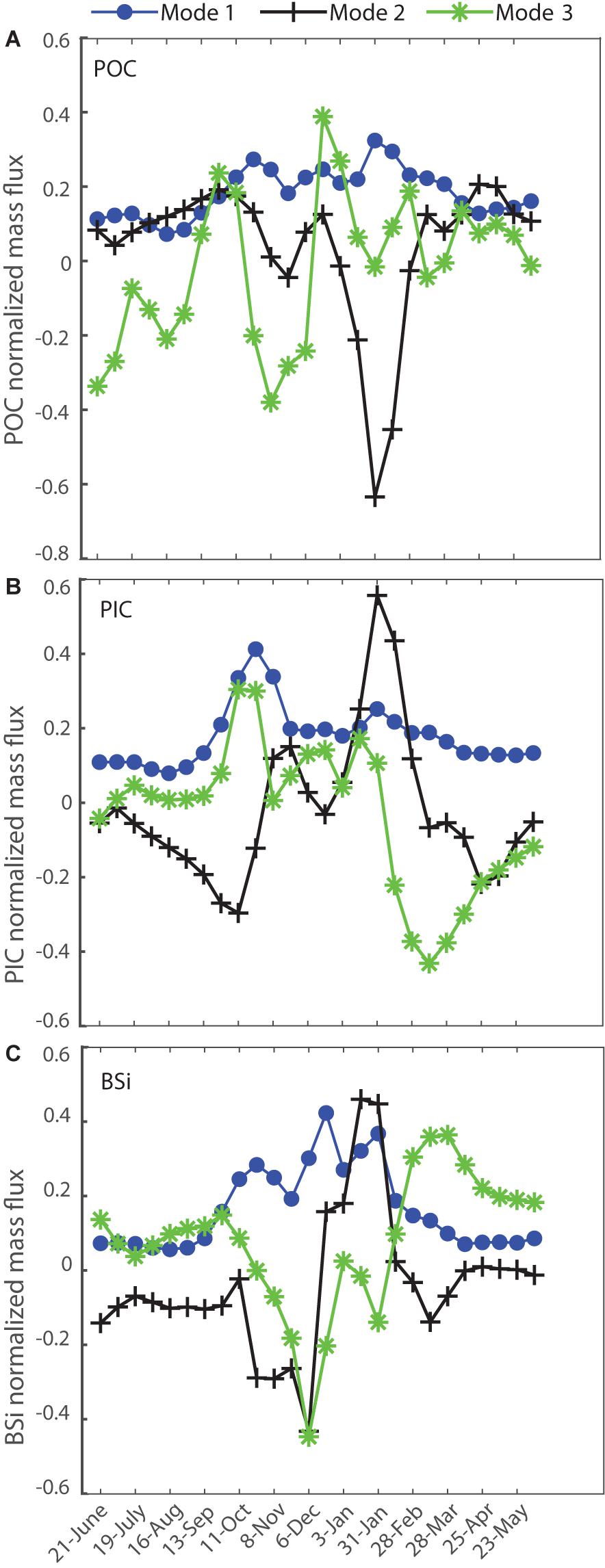
Figure 11. Singular Value Decomposition Modes for the particle component fluxes at 1000 m (A) POC, (B) PIC, (C) BSi.

With the SVD perspectives on seasonality in mind, we reconsider the FSI at SOTS. The interannual range in FSI of 43–144 days (43–114 at 1000 m, 54–144 at 2000 m, 94–143 at 3800 m) was similar to the global range reported by Lampitt and Antia (1997), and thus to the expectation of significant interannual variability in transfer efficiency. Figure 6 shows that interannual variation does occur, but is not correlated with FSI. The SVD shows that an overwhelming portion of the interannual flux variance is accounted for by the intensity of Mode 1, and thus that changes in the intra-seasonal temporal structure of the flux (as captured by the FSI) are not the most important driver of the interannual flux variations. In other words, results for all three depths indicate that the shape of the seasonal cycle is relatively consistent. This is consistent with the results that Modes 2 and 3, that describe changes in the seasonality, explain only small proportions of the interannual flux variance. In combination, the FSI and SVD analyses suggest that if trophic decoupling is a major driver of exported flux, then it must occur without changes in seasonality.

Possible Role of Net Primary Production in Control of Flux

A possible source of variability in annual flux is variability in NPP at the surface. Monthly estimates of NPP around the SOTS site (47°S and 142°E, with a square box around it of 1.5 degrees in both latitude and longitude, Figure 1) were obtained from the satellite-derived Vertically Generalized Production Model (VGPM, Behrenfeld and Falkowski, 1997) via the Oregon State University Ocean Productivity website², and assembled to provide integrated annual estimates of production. Figure 12, however, shows that there is no correlation between integrated annual production at the surface and integrated annual flux arriving at depth. Relative standard deviation of annual NPP between 2009 and 2016 was 10% compared to annual POC flux variability of 39% at 1000 m and 20% at 2000 m, which implies that export and/or attenuation may be more important controls than NPP. Recent assessments of satellite ocean color records have shown no statistically significant trends in either chlorophyll or derived NPP estimates in the SOTS region over the period 2003–2019, in keeping with the lack of trends in our observed fluxes at depth (Thompson and McDonald, 2020; Thompson et al., 2020).

FIGURE 12

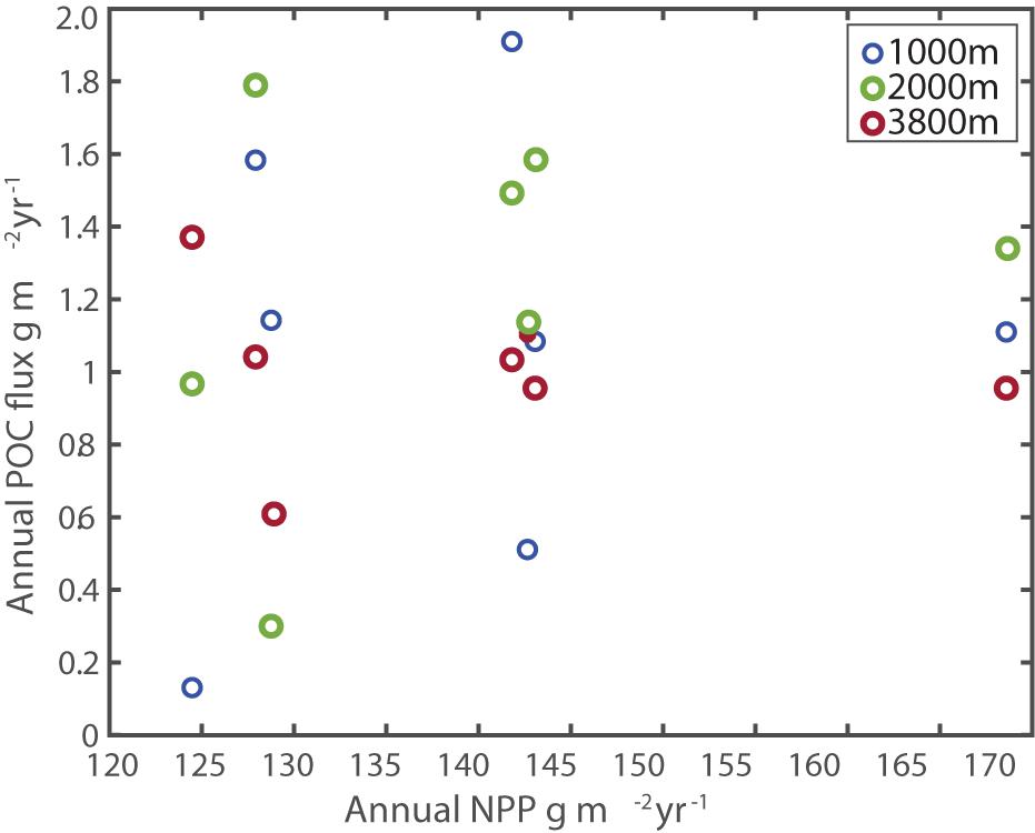
Figure 12. Comparison of Annual POC flux and Annual NPP at SOTS. No statistical correlation was observed at any depth.

Conclusion and Perspectives

After 20 years, SOTS is now one of the longest duration particle flux time series, particularly in the sparsely sampled Southern Ocean. Average POC fluxes across the three depths of 1.0 to 1.4 g m^–2 yr^–1 (1000–3800 m) recorded over the 20-year time series are comparable to previously measured values at the SOTS site (Trull et al., 2001b), other Subantarctic sites (Honjo et al., 2000; Nodder et al., 2016), the North Atlantic (Conte et al., 2001), the northeastern Subarctic Pacific (Wong et al., 1999) and the global median (Lampitt and Antia, 1997; Mouw et al., 2016). In contrast, the SOTS POC fluxes are lower than those of 2.5 g m^–2 yr^–1 for the polar North Pacific Ocean, 3.8 g m^–2 yr^–1 for the Pacific Sector of the Southern Ocean, 1.7 g m^–2 yr^–1 for the Atlantic Sector of the Southern Ocean, but larger than 0.6 g m^–2 yr^–1 for the Indian Sector of the Southern Ocean, as compiled by Lutz et al. (2007). The moderate interannual variability in total mass flux and the range in fluxes are similar to that of other long standing sediment trap time series (e.g., Ocean Station Papa in the Northeast Pacific, Wong et al., 1999).

No long-term trends in mass or POC fluxes can yet be seen beyond natural variability, which was also true for the 20-year time-series at BATS (Conte et al., 2001). This is consistent with expectations from a recent modeling study. Schlunegger et al. (2019) calculated the emergence time scales of anthropogenic impacts for a range of physical and biological processes, including a reduction in the strength of the soft-tissue pump as a consequence of reduced supply of nutrients to the surface ocean caused by changes in ocean circulation and stratification. The emergence timescale of this reduction is expected to be on the order of 23–50 years globally and up to 76 years locally. Schlunegger et al. (2019) also predicted a reduction in the calcium carbonate counter-pump to emerge in 10 years globally and 9-18 years regionally, but this depends on a strong response of biogenic carbonate production to carbonate saturation state (which has not been observed in field data in the Southern Ocean south of Australia, Trull et al., 2018).

Surface seasonality at SOTS is moderate, with no major autotrophic blooms (Eriksen et al., 2018) and small interannual variability in NPP (VGPM, Behrenfeld and Falkowski, 1997). The magnitude of NPP did not predict POC flux magnitude at depth on an annual timescale, possibly indicating that the mechanisms that affect export production and flux attenuation are more important than surface production. The lack of correlation between satellite derived surface productivity and POC flux at depth highlights the value of long-term direct measurements. In order to assess the importance of processes that link upper ocean productivity with carbon export versus remineralization during particle sinking on seasonal and interannual time scales, additional physical and biogeochemical water column parameters, are required. Some of these are available already from the SOTS program, and construction and validation of multiyear records are underway.

Interannual changes in flux seasonality were also moderate with a highly preserved seasonal structure and with most of the interannual variation explained by differences in flux magnitude that was not correlated with changes in seasonality. POC flux at depth was between 1 and 4% of NCP, at the lower end of values expected from commonly used attenuation models. The characteristic of moderate seasonality with significant interannual variations in the seasonal pattern but not the integrated annual fluxes, yet relatively constant annual fluxes is likely to be useful in selecting appropriate models for the simulation of environmental-ecological coupling and its role in controlling the biological carbon pump. Carbon export models for the SAZ need to be able to mechanistically reproduce the amplification of variability from ∼10% in surface NPP to 21–35% in POC flux at depth.

The Southern Ocean is a globally significant region for carbon export. The findings of this 20 year record, including the lack of any identifiable trends, will serve as an important baseline against which to measure future changes. Given the high proportion of biogenic carbonate minerals in the particle export, SOTS will be an important sentinel for the effects of both climate change and ocean acidification. The lack of correlation between satellite derived results of surface productivity and POC flux at depth may emphasize the importance of processes that control export production and flux attenuation. Our sediment trap based particle export time series is embedded in a wealth of data produced by the moorings, associated instruments, and service voyages at SOTS (see Eriksen et al., 2018; Trull et al., 2019 for further information on the diversity of observations). It is hoped that future work connecting our findings to locally measured environmental and biological parameters will shed additional light on the processes that control particle fluxes in the Southern Ocean.

Data Availability Statement

The raw data supporting the conclusions of this article will be made available by the authors, without undue reservation. Particle flux data is available through the IMOS AODN portal (https://portal.aodn.org.au/).

Author Contributions

All authors except ES, PJ, and RT performed the processing and chemical analyses of sediment trap samples. All authors except RT participated in voyage preparations and support during mooring servicing voyages. CW-E, ES, and TT analyzed and interpreted the time series results. RT provided the expertise on the singular value decomposition technique. CW-E, TT, and ES wrote the manuscript, with refinements contributed by all other authors.

Funding

This project has received grant funding from the Australian Government via many sources over the past two decades, including ship support from the Marine National Facility and Australian Antarctic Division, mooring equipment support from CSIRO and the Antarctic Climate and Ecosystems Cooperative Research Centre, and research staff support via all these agencies as well as the University of Tasmania and Australian Antarctic Program Partnership. RT was supported by a US NSF Graduate Research Fellowship. Support contributed by the USA National Science Foundation via the Woods Hole Oceanographic Institution was important to the initiation of the time series in 1997.

Conflict of Interest

The authors declare that the research was conducted in the absence of any commercial or financial relationships that could be construed as a potential conflict of interest.

Acknowledgments

We acknowledge support from the agencies Antarctic Climate and Ecosystems Cooperative Research Centre (ACE CRC), Integrated Marine Observing System (www.imos.org.au), University of Tasmania (UTAS), Bureau of Meteorology (BoM), Marine National Facility (MNF) and Australian Antarctic Division (AAD). Australia’s Integrated Marine Observing System (IMOS) is enabled by the National Collaborative Research Infrastructure Strategy (NCRIS). It is operated by a consortium of institutions as an unincorporated joint venture, with the University of Tasmania as Lead Agent. We also acknowledge the support of the CSIRO Marine and Atmospheric Research Moorings Group and Dr. Thomas Rodemann of Central Science Lab, UTAS for elemental analysis. SOTS is a member of the OceanSITES global network of time series observatories (www.OceanSITES.org). Thanks to Edward Doddridge for help with evaluation of singular value decomposition results, and Hugh Ducklow and Tyler Rohr for providing helpful comments that improved an earlier version of the manuscript.

Abbreviations

BSi, biogenic silicon; DOC, dissolved organic carbon; FSI, Flux Stability Index; NCP, net community production; NPP, net primary production; PIC, particulate inorganic carbon; POC, particulate organic carbon; POM, particulate organic matter; PN, particulate nitrogen; SAZ, subantarctic zone; SOTS, Southern Ocean Time Series; SVD, singular value decomposition.

Footnotes

1. ^ http://bats.bios.edu/bats-data/
2. ^ http://www.science.oregonstate.edu/ocean.productivity/index.php

References

Agassiz, A. (1888). Three cruises of the United States coast and Geodetic survey steamer Blake in the Gulf of Mexico, in the Caribbean sea, and along the Atlantic coast of the United States from 1877 to 1880. Bull. Museum Comp. Zool. Harvard 1, 1–314.

Google Scholar

Antia, A. N. (2005). Solubilization of particles in sediment traps: revising the stoichiometry of mixed layer export. Biogeosciences 2, 189–204. doi: 10.5194/bg-2-189-2005

CrossRef Full Text | Google Scholar

Archer, D., Winguth, A., Lea, D., and Mahowald, N. (2000). What caused the glacial/interglacial atmospheric pCO2 cycles? Biogeosciences 11, 1177–1198.

Google Scholar

Armstrong, R. A., Lee, C., Hedges, J. I., Honjo, S., and Wakeham, S. G. (2001). A new, mechanistic model for organic carbon fluxes in the ocean based on the quantitative association of POC with ballast minerals. Deep Sea Res. Part II Top. Stud. Oceanogr. 49, 219–236. doi: 10.1016/s0967-0645(01)00101-1

CrossRef Full Text | Google Scholar

Arteaga, L., Haentjens, N., Boss, E., Johnson, K. S., and Sarmiento, J. L. (2018). Assessment of export efficiency equations in the southern ocean applied to satellite-based net primary production. J. Geophys. Res. Oceans 123, 2945–2964. doi: 10.1002/2018jc013787

CrossRef Full Text | Google Scholar

Bach, L. T., Boxhammer, T., Larsen, A., Hildebrandt, N., Schulz, K. G., and Riebesell, U. (2016). Influence of plankton community structure on the sinking velocity of marine aggregates. Global Biogeochem. Cycles 30, 1145–1165. doi: 10.1002/2016gb005372

CrossRef Full Text | Google Scholar

Bach, L. T., Stange, P., Taucher, J., Achterberg, E. P., Alguero-Muniz, M., Horn, H., et al. (2019). The influence of plankton community structure on sinking velocity and remineralization rate of marine aggregates. Global Biogeochem. Cycles 33, 971–994. doi: 10.1029/2019gb006256

CrossRef Full Text | Google Scholar

Behrenfeld, M. J., and Falkowski, P. G. (1997). Photosynthetic rates derived from satellite-based chlorophyll concentration. Limnol. Oceanogr. 42, 1–20. doi: 10.4319/lo.1997.42.1.0001

CrossRef Full Text | Google Scholar

Berelson, W. M. (2002). Particle settling rates increase with depth in the ocean. Deep Sea Res. II 49, 237–251. doi: 10.1016/s0967-0645(01)00102-3

CrossRef Full Text | Google Scholar

Bopp, L., Monfray, P., Aumont, O., Dufresne, J. L., Le Treut, H., Madec, G., et al. (2001). Potential impact of climate change on marine export production. Global Biogeochem. Cycles 15, 81–99. doi: 10.1029/1999gb001256

CrossRef Full Text | Google Scholar

Bowie, A. R., Lannuzel, D., Remenyi, T. A., Wagener, T., Lam, P. J., Boyd, P. W., et al. (2009). Biogeochemical iron budgets of the Southern Ocean south of Australia: decoupling of iron and nutrient cycles in the subantarctic zone by the summertime sypply Global Biogeochem. Cycles 23:GB4034. 128.

Google Scholar

Boyd, P. W., Claustre, H., Levy, M., Siegel, D. A., and Weber, T. (2019). Multi-faceted particle pumps drive carbon sequestration in the ocean. Nature 568, 327–335. doi: 10.1038/s41586-019-1098-2

PubMed Abstract | CrossRef Full Text | Google Scholar

Boyd, P. W., and Trull, T. W. (2007). Understanding the export of biogenic particles in oceanic waters: Is there consensus? Progr. Oceanogr. 72, 276–312. doi: 10.1016/j.pocean.2006.10.007

CrossRef Full Text | Google Scholar

Boyd, P. W., Watson, A. J., Law, C. S., Abraham, E. R., Trull, T., Murdoch, R., et al. (2000). A mesoscale phytoplankton bloom in the polar Southern Ocean stimulated by iron fertilization. Nature 407, 695–702. doi: 10.1038/35037500

PubMed Abstract | CrossRef Full Text | Google Scholar

Bray, S. G., Trull, T. W., and Manganini, S. J. (2000). SAZ Project Moored Sediment Traps: Results of the 1997-1998 Deployments. Hobart, TAS: Antarct Coop. Res. Cent, 128.

Google Scholar

Buesseler, K. O., Antia, A. N., Chen, M., Fowler, S. W., Gardner, W. D., Gustafsson, O., et al. (2007a). An assessment of the use of sediment traps for estimating upper ocean particle fluxes. J. Mar. Res. 65, 345–416. doi: 10.1357/002224007781567621

CrossRef Full Text | Google Scholar

Buesseler, K. O., Lamborg, C. H., Boyd, P. W., Lam, P. J., Trull, T. W., Bidigare, R. R., et al. (2007b). Revisiting carbon flux through the ocean’s twilight zone. Science 316, 567–570.

Google Scholar

Cadzow, J. A., Baseghi, B., and Hsu, T. (1983). “Singular-value decomposition approach to time series modelling,” in IEE Proceedings F (Communications, Radar and Signal Processing), London: IET.

Google Scholar

Cardinal, D., Dehairs, F., Cattaldo, T., and André, L. (2001). Geochemistry of suspended particles in the Subantarctic and Polar Frontal Zones south of Australia: constraints on export and advection processes. J. Geophys. Res. Oceans 106, 31637–31656. doi: 10.1029/2000jc000251

CrossRef Full Text | Google Scholar

Carr, M.-E., Friedrichs, M. A., Schmeltz, M., Aita, M. N., Antoine, D., Arrigo, K. R., et al. (2006). A comparison of global estimates of marine primary production from ocean color. Deep Sea Res. Part II Top. Stud. Oceanogr. 53, 741–770.

Google Scholar

Closset, I., Cardinal, D., Bray, S. G., Thil, F., Djouraev, I., Rigual-Hernandez, A. S., et al. (2015). Seasonal variations, origin, and fate of settling diatoms in the Southern Ocean tracked by silicon isotope records in deep sediment traps. Global Biogeochem. Cycles 29, 1495–1510. doi: 10.1002/2015gb005180

CrossRef Full Text | Google Scholar

Conte, M. H., Ralph, N., and Ross, E. H. (2001). Seasonal and interannual variability in deep ocean particle fluxes at the Oceanic Flux Program (OFP)/Bermuda Atlantic Time Series (BATS) site in the western Sargasso Sea near Bermuda. Deep-Sea Res. II 48, 1471–1505. doi: 10.1016/s0967-0645(00)00150-8

CrossRef Full Text | Google Scholar

Copin-Montegut, C., and Copin-Montegut, G. (1983). Stoichiometry of carbon, nitrogen, and phosphorus in marine particulate matter. Deep Sea Res. Part A Oceanogr. Res. Pap. 30, 31–46. doi: 10.1016/0198-0149(83)90031-6

CrossRef Full Text | Google Scholar

Cram, J. A., Weber, T., Leung, S. W., McDonnell, A. M. P., Liang, J.-H., et al. (2018). The role of particle size, ballast, temperature, and oxygen in the sinking flux to the deep sea. Global Biogeochem. Cycles 858–876. doi: 10.1029/2017gb005710

CrossRef Full Text | Google Scholar

DeVries, T., Primeau, F., and Deutsch, C. (2012). The sequestration efficiency of the biological pump. Geophys. Res. Lett. 39:5.

Google Scholar

DeVries, T., and Weber, T. (2017). The export and fate of organic matter in the ocean: new constraints from combining satellite and oceanographic tracer observations. Global Biogeochem. Cycles 31, 535–555. doi: 10.1002/2016gb005551

CrossRef Full Text | Google Scholar

Ducklow, H. W. (1995). Ocean biogeochemical fluxes: new production and export of organic matter from the upper ocean. Rev. Geophys. 33, 1271–1276. doi: 10.1029/95rg00130

CrossRef Full Text | Google Scholar

Ducklow, H. W., Erickson, M., Kelly, J., Montes-Hugo, M., Ribic, C. A., Smith, R. C., et al. (2008). Particle export from the upper ocean over the continental shelf of the west Antarctic Peninsula: a long-term record, 1992–2007. Deep Sea Res. Part II Top. Stud. Oceanogr. 55, 2118–2131. doi: 10.1016/j.dsr2.2008.04.028

CrossRef Full Text | Google Scholar

Dugdale, R. C., Wilkerson, F. P., and Minas, H. J. (1995). The role of a silicate pump in driving new production. Deep Sea Res. Part I Oceanogr. Res. Pap. 42, 697–719. doi: 10.1016/0967-0637(95)00015-x

CrossRef Full Text | Google Scholar

Ebersbach, F., Trull, T. W., Davies, D. M., and Bray, S. G. (2011). Controls on mesopelagic particle fluxes in the Sub-Antarctic and Polar Frontal Zones in the Southern Ocean south of Australia in summer—Perspectives from free-drifting sediment traps. Deep Sea Res. Part II Top. Stud. Oceanogr. 58, 2260–2276. doi: 10.1016/j.dsr2.2011.05.025

CrossRef Full Text | Google Scholar

Eriksen, R., Trull, T. W., Davies, D., Jansen, P., Davidson, A. T., Westwood, K., et al. (2018). Seasonal succession of phytoplankton community structure from autonomous sampling at the Australian Southern Ocean Time Series site. Mar. Ecol. Progr. Ser. 589, 13–31. doi: 10.3354/meps12420

CrossRef Full Text | Google Scholar

Evans, G. T., and Parslow, J. S. (1985). A model of annual plankton cycles. Biol. Oceanogr. 3, 327–347.

Google Scholar

Falkowski, P., Scholes, R., Boyle, E., Canadell, J., Canfield, D., Elser, J., et al. (2000). The global carbon cycle: a test of our knowledge of earth as a system. Science 290, 291–296. doi: 10.1126/science.290.5490.291

PubMed Abstract | CrossRef Full Text | Google Scholar

Falkowski, P. G., Barber, R. T., and Smetacek, V. (1998). Biogeochemical controls and feedbacks on ocean primary production. Science 281, 200–206. doi: 10.1126/science.281.5374.200

PubMed Abstract | CrossRef Full Text | Google Scholar

Feely, R. A., Sabine, C. L., Lee, K., Berelson, W., Kleypas, J., Fabry, V. J., et al. (2004). Impact of anthropogenic CO2 on the CaCO3 system in the oceans. Science 305, 362–366. doi: 10.1126/science.1097329

PubMed Abstract | CrossRef Full Text | Google Scholar

Frankignoulle, M., and Gattuso, J. (1993). “Air-sea CO2 exchange in coastal ecosystems,” in Interactions of C, N, P and S Biogeochemical Cycles and Global Change. NATO ASI Series (Series I: Global Environmental Change), eds R. Wollast, F. T. Mackenzie, and L. Chou (Heidelberg: Springer), 4.

Google Scholar

Gardner, W. D. (1985). The effect of tilt on sediment trap efficiency. Deep-Sea Res. 32, 349–361. doi: 10.1016/0198-0149(85)90083-4

CrossRef Full Text | Google Scholar

Gehlen, M., Bopp, L., Emprin, N., Aumont, O., Heinze, C., and Ragueneau, O. (2006). Reconciling surface ocean productivity, export fluxes and sediment composition in a global biogeochemical ocean model. Biogeosciences 3, 521–537. doi: 10.5194/bg-3-521-2006

CrossRef Full Text | Google Scholar

Guidi, L., Stemmann, L., Jackson, G. A., Ibanez, F., Claustre, H., Legendre, L., et al. (2009). Effects of phytoplankton community on production, size and export of large aggregates: a world-ocean analysis. Limnol. Oceanogr. 54, 1951–1963. doi: 10.4319/lo.2009.54.6.1951

CrossRef Full Text | Google Scholar

Hamilton, K. M. (2006). Evaluating the Consistency of Satellite and Deep Sediment Trap Carbon Export Data in the Southern Ocean. Institute of Antarctic and Southern Ocean Studies (IASOS). Hobart: University of Tasmania. Bachelor of Science.

Google Scholar

Helm, K. P., Bindoff, N. L., and Church, J. A. (2011). Observed decreases in oxygen content of the global ocean. Geophys. Res. Lett. 38, L23602.

Google Scholar

Henson, S. A., Sanders, R., and Madsen, E. (2012). Global patterns in efficiency of particulate organic carbon export and transfer to the deep ocean. Global Biogeochem. Cycles 26:GB1028.

Google Scholar

Herraiz-Borreguero, L., and Rintoul, S. R. (2011). Regional circulation and its impact on upper ocean variability south of Tasmania (Australia). Deep-Sea Res. II 58, 2071–2081. doi: 10.1016/j.dsr2.2011.05.022

CrossRef Full Text | Google Scholar

Honda, M. C., and Watanabe, S. (2010). Importance of biogenic opal as ballast of particulate organic carbon (POC) transport and existence of mineral ballast-associated and residual POC in the Western Pacific Subarctic Gyre. Geophys. Res. Lett. 37:L02605.

Google Scholar

Honjo, S., Francois, R., Manganini, S., Dymond, J., and Collier, R. (2000). Particle fluxes to the interior of the Southern Ocean in the Western Pacific sector along 170°W. Deep Sea Res. II 47, 3521–3548. doi: 10.1016/s0967-0645(00)00077-1

CrossRef Full Text | Google Scholar

Honjo, S., and Manganini, S. J. (1993). Annual biogenic particle fluxes to the interior of the North Atlantic Ocean; studied at 34°N 21°W and 48°N 21°W. Deep Sea Res. I 40, 587–607. doi: 10.1016/0967-0645(93)90034-k

CrossRef Full Text | Google Scholar

Honjo, S., Manganini, S. J., Krishfield, R. A., and Francois, R. (2008). Particulate organic carbon fluxes to the ocean interior and factors controlling the biological pump: a synthesis of global sediment trap programs since 1983. Progr. Oceanogr. 76, 217–285. doi: 10.1016/j.pocean.2007.11.003

CrossRef Full Text | Google Scholar

Jacquet, S., Lam, P., Trull, T., and Dehairs, F. (2011). Carbon export production in the subantarctic zone and polar front zone south of Tasmania. Deep Sea Res. Part II Top. Stud. Oceanogr. 58, 2277–2292. doi: 10.1016/j.dsr2.2011.05.035

CrossRef Full Text | Google Scholar

Johnson, R., Strutton, P. G., Wright, S. W., McMinn, A., and Meiners, K. M. (2013). Three improved satellite chlorophyll algorithms for the Southern Ocean. J. Geophys. Res. Oceans 118, 3694–3703.

Google Scholar

Johnson, R., and Pacheco, F. (1998-2016). Bermuda atlantic time-series study (BATS) sediment trap data. Retrieved 1:2020.

Google Scholar

Kim, H., Doney, S. C., Iannuzzi, R. A., Meredith, M. P., Martinson, D. G., and Ducklow, H. W. (2016). Climate forcing for dynamics of dissolved inorganic nutrients at Palmer Station, Antarctica: an interdecadal (1993–2013) analysis. J. Geophys. Res. Biogeosci. 121, 2369–2389. doi: 10.1002/2015jg003311

CrossRef Full Text | Google Scholar

King, A. L., and Howard, W. R. (2003). Planktonic foraminiferal flux seasonality in Subantarctic sediment traps: a test for paleoclimate reconstructions. Paleoceanography 18:1019.

Google Scholar

Klaas, C., and Archer, D. E. (2002). Association of sinking organic matter with various types of mineral ballast in the deep sea: implications for the rain ratio. Global Biogeochem. Cycles 16:14.

Google Scholar

Lampitt, R. S., and Antia, A. N. (1997). Particle flux in deep seas: regional characteristics and temporal variability. Deep Sea Res. I 44, 1377–1403. doi: 10.1016/s0967-0637(97)00020-4

CrossRef Full Text | Google Scholar

Lannuzel, D., Bowie, A. R., Lam, P., Townsend, A., Ibisanmi, E., Butler, E., et al. (2011). Distribution of dissolved and particulate iron in the sub-Antarctic and Polar Frontal Southern Ocean (astralian sector). Deep Sea Res. II 58, 2094–2112. doi: 10.1016/j.dsr2.2011.05.027

CrossRef Full Text | Google Scholar

Lee, K., Wanninkhof, R., Takahashi, T., Doney, S. C., and Feely, R. A. (1998). Low interannual variability in recent oceanic uptake of atmospheric carbon dioxide. Nature 396, 155–159. doi: 10.1038/24139

CrossRef Full Text | Google Scholar

Lima, I. D., Lam, P. J., and Doney, S. C. (2014). Dynamics of particulate organic carbon flux in a global ocean model. Biogeosciences 11, 1177–1198. doi: 10.5194/bg-11-1177-2014

CrossRef Full Text | Google Scholar

Lindemann, C., and St John, M. A. (2014). A seasonal diary of phytoplankton in the North Atlantic. Front. Mar. Sci. 1:37. doi: 10.3389/fmars.2014.00037

CrossRef Full Text | Google Scholar

Lourey, M. J., and Trull, T. W. (2001). Seasonal nutrient depletion and carbon export in the subantarctic and polar frontal zones of the Southern Ocean south of Australia. J. Geophys. RES. 106, 31463–31487. doi: 10.1029/2000jc000287

CrossRef Full Text | Google Scholar

Lutz, M. J., Caldeira, K., Dunbar, R. B., and Behrenfeld, M. J. (2007). Seasonal rhythms of net primary production and particulate organic carbon flux to depth describe the efficiency of biological pump in the global ocean. J. Geophys. Res. 112:C10011.

Google Scholar

Maiti, K., Charette, M. A., Buesseler, K. O., and Kahru, M. (2013). An inverse relationship between production and export efficiency in the Southern Ocean. Geophys. Res. Lett. 40, 1557–1561. doi: 10.1002/grl.50219

CrossRef Full Text | Google Scholar

Manno, C., Giglio, F., Stowasser, G., Fielding, S., Enderlein, P., and Tarling, G. (2018). Threatened species drive the strength of the carbonate pump in the northern Scotia Sea. Nat. Commun. 9, 1–7.

Google Scholar

Martin, J. H., Knauer, G. A., Karl, D. M., and Broenkow, W. W. (1987). VERTEX: carbon cycling in the northeast Pacific. Deep-Sea Res. 34, 267–285. doi: 10.1016/0198-0149(87)90086-0

CrossRef Full Text | Google Scholar

Meijers, A., Bindoff, N., and Rintoul, S. (2011). Estimating the four-dimensional structure of the Southern Ocean using satellite altimetry. J. Atmos. Oceanic Technol. 28, 548–568. doi: 10.1175/2010jtecho790.1

CrossRef Full Text | Google Scholar

Metzl, N., Tilbrook, B., and Poisson, A. (1999). The annual fCO2 cycel and the air-sea CO2 flux in the sub-Antarctic Ocean. Tellus Ser. B. 51, 849–861. doi: 10.1034/j.1600-0889.1999.t01-3-00008.x

PubMed Abstract | CrossRef Full Text | Google Scholar

Morel, F. M., Rueter, J. G., and Price, N. M. (1991). Iron nutrition of phytoplankton and its possible importance in the ecology of ocean regions with high nutrient and low biomass. Oceanography 4, 56–61. doi: 10.5670/oceanog.1991.03

CrossRef Full Text | Google Scholar

Mouw, C. B., Barnett, A., McKinley, G. A., Gloege, L., and Pilcher, D. (2016). Global ocean particulate organic carbon flux merged with satellite parameters. Earth Syst. Sci. Data 8, 531–541. doi: 10.5194/essd-8-531-2016

CrossRef Full Text | Google Scholar

Moy, A. D., Howard, W. R., Bray, S. G., and Trull, T. W. (2009). Reduced calcification in modern Southern Ocean planktonic foraminifera. Nat. Geosci. 2, 276–280. doi: 10.1038/ngeo460

CrossRef Full Text | Google Scholar

Nodder, S. D., Chiswell, S. M., and Northcote, L. C. (2016). Annual cycles of deep-ocean biogeochemical export fluxes in subtropical and subantarctic waters, southwest Pacific Ocean. J. Geophys. Res. 121, 2405–2424. doi: 10.1002/2015jc011243

CrossRef Full Text | Google Scholar

Orr, J. C., Fabry, V. J., Aumont, O., Bopp, L., Doney, S. C., and Feely, R. A. (2005). Anthropogenic ocean acidification over the twenty-first century and its impact on calcifying organisms. Nature 437, 681–696.

Google Scholar

Redfield, A. C. (1963). The influence of organisms on the composition of seawater. Sea 2, 26–77.

Google Scholar

Rees, C., Lindsay, P., Sherrin, K., Schwanger, C., Hughes, P., Tibben, S., et al. (2018). Methods for reproducible shipboard SFA nutrient measurement using RMNS and automated data processing. Limnol. Oceanogr. Methods 17, 25–41.

Google Scholar

Rigual Hernández, A. S., Trull, T. W., Nodder, S. D., Flores, J. A., Bostock, H., Abrantes, F., et al. (2019). Coccolithophore biodiversity controls carbonate export in the Southern Ocean. Biogeosci. Discuss. 17, 245–263. doi: 10.5194/bg-17-245-2020

CrossRef Full Text | Google Scholar

Rigual-Hernández, A., Trull, T., Bray, S., Cortina, A., and Armand, L. (2015). Latitudinal and temporal distributions of diatom populations in the pelagic waters of the Subantarctic and Polar Frontal zones of the Southern Ocean and their role in the biological pump. Biogeosciences 12, 5309–5337. doi: 10.5194/bg-12-5309-2015

CrossRef Full Text | Google Scholar

Rigual-Hernández, A., Trull, T., Flores, J., Nodder, S., Eriksen, R., Davies, D., et al. (2020). Full annual monitoring of Subantarctic Emiliania huxleyi populations reveals highly calcified morphotypes in high-CO2 winter conditions. Sci. Rep. 10, 1–14.

Google Scholar

Rintoul, S. R., and Trull, T. W. (2001). Seasonal evolution of the mixed layer in the Subantarctic Zone south of Australia. J. Geophys. Res. Oceans 106, 31447–31462. doi: 10.1029/2000jc000329

CrossRef Full Text | Google Scholar

Roberts, D., Hopcroft, R. R., and Hosie, G. W. (2014). “6.4. southern ocean pteropods,” in Biogeographic Atlas of the Southern Ocean, Vol.XII, eds C. De Broyer, P. Koubbi, H. J. Griffiths, et al. (Cambridge: Scientific Committee on Antarctic Research), 276–283.

Google Scholar

Rost, B., and Riebesell, U. (2004). Coccolithophores and the Biological Pump: Responses to Environmental Changes. Coccolithophores. Berlin: Springer, 99–125.

Google Scholar

Salter, I., Schiebel, R., Ziveri, P., Movellan, A., Lampitt, R., and Wolff, G. A. (2014). Carbonate counter pump stimulated by natural iron fertilization in the Polar Frontal Zone. Nat. Geosci. 7, 885–889. doi: 10.1038/ngeo2285

CrossRef Full Text | Google Scholar

Sarmiento, J. L., Hughes, T. M. C., Stouffer, R. J., and Manabe, S. (1998). Simulated response of the ocean carbon cycle to anthropogenic climate warming. Nature 393, 245–249. doi: 10.1038/30455

CrossRef Full Text | Google Scholar

Sarmiento, J. L., and LeQuere, C. (1996). Oceanic carbon dioxide uptake in a model of century-scale global warming. Science 274, 1346–1350. doi: 10.1126/science.274.5291.1346

PubMed Abstract | CrossRef Full Text | Google Scholar

Schlunegger, S., Rodgers, K. B., Sarmiento, J. L., Frölicher, T. L., Dunne, J. P., Ishii, M., et al. (2019). Emergence of anthropogenic signals in the ocean carbon cycle. Nat. Clim. Change 9, 719–725. doi: 10.1038/s41558-019-0553-2

PubMed Abstract | CrossRef Full Text | Google Scholar

Schneider, B., Schlitzer, R., Fischer, G., and Nöthig, E. M. (2003). Depth-dependent elemental compositions of particulate organic matter (POM) in the ocean. Global Biogeochem. Cycles 17, 1–16.

Google Scholar

Shadwick, E. H., Trull, T. W., Tilbrook, B., Sutton, A. J., Schulz, E., and Sabine, C. L. (2015). Seasonality of biological and physical controls on surface ocean CO2 from hourly observations at the Southern Ocean Time Series site south of Australia. Global Biogeochem. Cycles 29, 1–16.

Google Scholar

Shaffer, G. (1993). Effects of the Marine Carbon Biota on Global Carbon Cycling. The Global Carbon Cycle, eds M. Heimann. New York, NY: Springer-Verlag, 431–435.

Google Scholar

Siegel, D. A., Granata, T. C., Michaels, A. F., and Dickey, T. D. (1990). Mesoscale eddy diffusion, particle sinking, and the interpretation of sediment trap data. J. Geophys. Res. Oceans 95, 5305–5311.

Google Scholar

Sigman, D. M., and Boyle, E. A. (2000). Glacial/Interglacial variations in atmospheric carbon dioxide. Nature 407, 859–869. doi: 10.1038/35038000

PubMed Abstract | CrossRef Full Text | Google Scholar

Suess, E. (1980). Particulate organic carbon flux in the oceans—surface productivity and oxygen utilization. Nature 288, 260–263. doi: 10.1038/288260a0

CrossRef Full Text | Google Scholar

Thompson, P., and McDonald, K. (2020). “Spatial and seasonal trends in net primary production,” in State and Trends of Australia’s Ocean Report, eds A. J. Richardson, R. Eriksen, T. Moltmann, I. Hodgson-Johnston, and J. R. Wallis (Hobart: Integrated Marine Observing System), 1–5.

Google Scholar

Thompson, P., Antoine, D., and King, E. (2020). “Spatial and seasonal trends in chlorophyll a,” in State and Trends of Australia’s Ocean Report, eds A. J. Richardson, R. Eriksen, T. Moltmann, I. Hodgson-Johnston, and J. R. Wallis (Hobart: Integrated Marine Observing System), 1–5.

Google Scholar

Trinh, R., and Ducklow, H. (2018). “Years of particle export in west antarctic peninsula coastal waters,” in Proceedings from Polar 2018 A SCAR & IASC Conference, Davos.

Google Scholar

Trull, T., Rintoul, S. R., Hadfield, M., and Abraham, E. R. (2001a). Circulation and seasonal evolution of polar waters south of Australia: implications for iron fertilization of the Southern Ocean. Deep Sea Res. Part II Top. Stud. Oceanogr. 48, 2439–2466. doi: 10.1016/s0967-0645(01)00003-0

CrossRef Full Text | Google Scholar

Trull, T. W., Bray, S. G., Manganini, S. J., Honjo, S., and Francois, R. (2001b). Moored sediment trap measurements of carbon export in the Subantarctic and Polar Frontal Zones of the Southern Ocean, south of Australia. J. Geophys. Res. 106, 31489–31506.

Google Scholar

Trull, T. W., Sedwick, P. N., Griffiths, F. B., and Rintoul, S. R. (2001c). Introduction to special edition: SAZ Project. J. Geophys. Res. 106, 31425–31429. doi: 10.1029/2001jc001008

CrossRef Full Text | Google Scholar

Trull, T. W., Bray, S. G., Buesseler, K. O., Lamborg, C. H., Manganini, S. J., Moy, C., et al. (2008). In situ measurements of mesopelagic particle sinking rates and the control of carbon transfer to the ocean interior during the Vertical Flux in the Global Ocean (VERTIGO) voyages in the North Pacific. Deep-Sea Res. II 55, 1684–1695. doi: 10.1016/j.dsr2.2008.04.021

CrossRef Full Text | Google Scholar

Trull, T. W., Jansen, P., Schulz, E., Weeding, B., Davies, D. M., and Bray, S. G. (2019). Autonomous multi-trophic observations of productivity and export at the Australian Southern Ocean Time Series (SOTS) reveal sequential mechanisms of physical-biological coupling. Front. Mar. Sci. 6:525. doi: 10.3389/fmars.2019.00525

CrossRef Full Text | Google Scholar

Trull, T. W., Passmore, A., Davies, D. M., Smit, T., Berry, K., and Tilbrook, B. (2018). Distribution of planktonic biogenic carbonate organisms in the Southern Ocean south of Australia: a baseline for ocean acidification impact assessment. Biogeosciences 15, 31–49. doi: 10.5194/bg-15-31-2018

CrossRef Full Text | Google Scholar

Volk, T., and Hoffert, M. I. (1985). Ocean Carbon Pumps: Analysis of Relative Strengths and Efficiencies in Ocean-Driven Atmospheric CO2 Changes. The Carbon Cyclen and Atmospheric CO2: Natural variations archean to present, eds E. Sundquist and W.S. Broecker. Washington, DC: AGU, 99–110.

Google Scholar

Weber, T., Cram, J. A., Leung, S. W., DeVries, T., and Deutsch, C. (2016). Deep ocean nutrients imply large latitudinal variation in particle transfer efficiency. Proc. Natl. Acad. Sci. U.S.A. 113, 8606–8611. doi: 10.1073/pnas.1604414113

PubMed Abstract | CrossRef Full Text | Google Scholar

Weeding, B., and Trull, T. W. (2014). Hourly oxygen and total gas tension measurements at the Southern Ocean Time Series site reveal winter ventilation and spring net community production. J. Geophys. Res. Oceans 119, 348–358. doi: 10.1002/2013jc009302

CrossRef Full Text | Google Scholar

Wong, C., Whitney, F., Crawford, D., Iseki, K., Matear, R., Johnson, W., et al. (1999). Seasonal and interannual variability in particle fluxes of carbon, nitrogen and silicon from time series of sediment traps at Ocean Station P, 1982–1993: relationship to changes in subarctic primary productivity. Deep Sea Res. Part II Top. Stud. Oceanogr. 46, 2735–2760. doi: 10.1016/s0967-0645(99)00082-x

CrossRef Full Text | Google Scholar

Wynn-Edwards, C. A., Davies, D. M., Jansen, P., Bray, S. G., Eriksen, R., and Trull, T. W. (2019). Southern Ocean Time Series. SOTS Annual Reports: 2012/2013. Report 2. Samples. IMOS – ABOS Southern Ocean Time Series (SOTS) – Annual Reports. Canberra: CSIRO. Available online at: https://catalogue-imos.aodn.org.au/geonetwork/srv/api/records/afc166ce-6b34-44d9-b64c-8bb10fd43a07

Google Scholar

Wynn-Edwards, C. A., Davies, D. M., Shadwick, E. H., and Trull, T. W. (2020). Southern Ocean Time Series. SOTS Quality assessment and control report. Sediment trap particle fluxes Version 1.0. IMOS – Integrated Marine Observing System. Canberra: CSIRO.

Google Scholar

Yoder, J. A., and Kennelly, M. A. (2003). Seasonal and ENSO variability in global ocean phytoplankton chlorophyll derived from 4 years of SeaWiFS measurements. Global Biogeochem. Cycles 17:1112.

Google Scholar

Yu, E.-F., Francois, R., Bacon, M. P., Honjo, S., Fleer, A. P., Manganini, S. J., et al. (2001). Trapping efficiency of bottom-tethered sediment traps estimated from the intercepted fluxes of 230Th and 231Pa. Deep-Sea Res. Part 1, 865–889. doi: 10.1016/s0967-0637(00)00067-4

CrossRef Full Text | Google Scholar