Response of Ozone to a Gravity Wave Process in the UTLS Region Over the Tibetan Plateau

In this paper, ERA5 reanalysis data from the European Center for Medium-Range Weather Forecasts and the Weather Research and Forecasting (WRF) mesoscale model are used to compare and simulate a topographic gravity wave event that occurred over the Tibetan Plateau between 18:00 on 3 May 2014 and 00:00 on 4 May 2014. The stratosphere–troposphere exchange (STE) process and its detailed characteristics during the gravity wave event are presented. The response of the upper troposphere and lower stratosphere (UTLS) ozone to the gravity wave is discovered from the perspective of the gravity wave dynamic process. The results show that the gravity wave structure between 90°E and 100°E had a westward tilt with height. From 19:00 to 21:00 the gravity waves decayed and from 22:00 to 23:00 their shape gradually blurred. Meanwhile, there was a response of the ozone mixing ratio in the UTLS over the Tibetan Plateau to the gravity waves breaking. After 21:00, this wave process caused the STE, as air from the stratosphere with a greater ozone concentration was injected into the upper troposphere, leading to rapidly increased ozone concentration there.

Introduction

The processes in the upper troposphere and lower stratosphere (UTLS) play a significant role in weather and climate (Bian et al., 2020). Ozone in the UTLS has an important impact on global climate change and directly or indirectly changes the thermal structure and components of the atmosphere (Xia et al., 2018; Wang et al., 2020). In the early 1970s, scientists issued warnings for the first time that stratospheric ozone could be threatened by chlorofluorocarbons (CFCs) and other anthropogenic substances (Crutzen, 1970; Molina and Rowland, 1974). However, their work was not valued by the scientific community at the time until the discovery of the Antarctic ozone hole in 1985 (Farman et al., 1985), caused great shock to governments, the scientific community, and the media. The high chlorine content in the Antarctic ozone hole confirmed the theories of Crutzen and Molina, and Rowland, and its discovery led to the signing of the Montreal Protocol on the control of ozone-depleting substances in 1987. Later, in 1995, Crutzen, Molina, and Rowland won the Nobel Prize for Chemistry.

In fact, ozone depletion does not only exist in polar regions. In 1995, Zhou first discovered that there was a low ozone center in the boreal summer over the Tibetan Plateau (Zhou and Luo, 1994), and this third low-ozone region—after the North and South Poles—became a hot spot of worldwide attention. In 2017, further studies verified the reliability of satellite remote sensing of the ozone profile over the Tibetan Plateau (Shi et al., 2017b). According to an environmental survey report released by the Tibet Autonomous Region, the thinning of the ozone layer has caused an increasingly high proportion of ultraviolet radiation, which has led to light pollution of the atmospheric environment. In addition, snow and rock cause strong reflection of ultraviolet radiation, which has resulted in year on year increases in the incidence rate of cataracts, a leading cause of blindness, in the population of the Tibet area. At present, the incidence rate of cataracts in Tibet is the highest in China (see, for example, the Chinese popular science website, http://www.kepu.cn/vmuseum/earth/weather/pollution/plt033.html). Therefore, studying the formation mechanism of ozone over the Tibetan Plateau is not only important for human survival, but can also provide a basis for beneficial changes in weather, climate, and meteorological pollution.

Research shows show that there are three main causes of low ozone values over the Tibetan Plateau: dynamic effects of the atmosphere, large-scale orography, and atmospheric chemical reactions. Among these, the dynamic transmission of the atmosphere plays the major role (Tian et al., 2008; Zhang et al., 2014; Guo et al., 2017). These dynamic effects mainly include circulation anomalies caused by thermal forcing (Zhang et al., 2014), large-scale ascending and sinking motions on the isentropic surface (Tian et al., 2008), stratosphere–troposphere exchange (STE; Zhou et al., 2004), and the Asian monsoon (Bian et al., 2011).

Connections between the troposphere and stratosphere are always caused by waves, for example planetary waves (Shi et al., 2017a) and gravity waves. An atmospheric gravity wave is a disturbance phenomenon with vertical propagation properties which plays an important role in global meteorology, climatology, chemistry, and stratosphere dynamics (Holton, 1983; Fetzer and Gille, 1994; Bai et al., 2017). With the development of observational methods (Chang et al., 2020; Mai et al., 2020; Sheng et al., 2020), gravity waves can now be extracted in different ways (He et al., 2020). The most important sources of gravity waves include topography, convection, and wind shear. Previous studies have shown that the breaking process of atmospheric gravity waves is an important driving force of small-scale turbulent mixing in the middle and upper atmosphere (Miyazaki et al., 2010). Meanwhile, the development and breaking processes of gravity waves can also result in mass exchange (Pan et al., 2010). The Tibetan Plateau is a key STE area (Zhou et al., 2004; Shi et al., 2018). However, the response of ozone in the UTLS region over the Tibetan Plateau to topographic gravity waves has not previously been examined in detail. In the polar region, studies have shown that topographic gravity waves can affect stratospheric ozone via chemical reactions on polar stratospheric cloud (PSC) particles (Carslaw et al., 1998; Spang et al., 2018). Wei et al. (2016) have studied the impact of orographic gravity wave on UTLS ozone, but the detailed characteristics have not been described. Therefore, exploring the response of ozone in the UTLS to gravity waves from the perspective of gravity wave dynamic processes is necessary and valuable work.

Previous related studies have shown that the Weather Research and Forecasting (WRF) model is capable of simulating mesoscale gravity wave signals; for example, Chen et al. (2012, 2013) used the WRF model to simulate the process of a typhoon-induced stratospheric gravity wave. In this paper, ERA5 reanalysis data from the European Center for Medium-Range Weather Forecasts (ECMWF) and the WRF mesoscale model are used to analyze a topographic gravity wave event that occurred over the Tibetan Plateau. The response of ozone in the UTLS region to this gravity wave event is obtained and the details of the STE process are given, providing scientific basis for further research.

Data, Methods, and Numerical Simulation Scheme

Gravity Wave Selection

The gravity wave event analyzed in this paper occurred over the Tibetan Plateau between 18:00 UTC on 3 May 2014 and 00:00 UTC on 4 May 2014. Top-down satellite perspectives can provide a practical means to remotely gather gravity wave information (Miller et al., 2015). Figure 1A shows the Visible Infrared Imaging Radiometer Suite (VIIRS) thermal infrared (10.76 μm) imagery of the Himalayas and the Tibetan Plateau at 19:22 UTC on 3 May 2014. The location of the cloud can be seen from Figure 1A. The corresponding Day/Night Band (DNB) visible/near-infrared imagery is shown in Figure 1B. The DNB radiometer was located on the Suomi National Polar-orbiting Partnership (NPP; hereafter, Suomi) satellite. The waves are far removed from the bright city lights emanating from the densely populated Indian districts. We can clearly recognize the structure of the gravity wave fluctuation in the roughly northwest/southeast-oriented bands in the portion of the image outlined in yellow. In fact, observations of mountain waves over this largely inaccessible area are rare (Miller et al., 2015), but we can recognize the wave structure based on the DNB. Is there a response in the ozone mixing ratio in the UTLS to the breaking of the gravity waves? In this article we analyze that question.

FIGURE 1

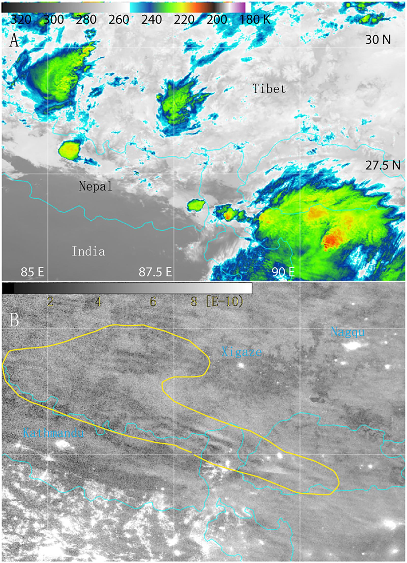
Figure 1. (A) VIIRS thermal infrared (10.76 μm) image over the Tibetan Plateau at 19:22 on 3 May 2014; (B) The visible/near-infrared image of the corresponding Suomi satellite DNB; the yellow outline shows the central signal area of the gravity wave (Miller et al., 2015).

For our study, we first took the gravity wave signal and ozone distributions obtained from ERA5 reanalysis data and then used the WRF model to simulate the gravity wave process. The ERA5 reanalysis data used in this paper have a spatial resolution of 0.25 × 0.25, and the vertical level is from 1000 hPa to 1 hPa, with 37 layers in total. We used the temperature, pressure, wind speed, and ozone mixing ratio data from 18:00 on 3 May, 2014 to 00:00 on 4 May, 2014 for calculation and analysis.

Numerical Simulation Scheme

The Advanced Research WRF (WRF-ARW) v.4.0.1 mesoscale model is a new-generation prediction model and assimilation system jointly developed by the National Center for Atmospheric Research (NCAR), the National Centers for Environmental Prediction (NCEP), and the Center for Analysis and Prediction of Storms (CAPS) at the University of Oklahoma.

In order to obtain detailed characteristics of the selected gravity wave process, we used the WRF model to simulate this gravity wave. Using a Lambert projection, the area range was 75°E–115°E, 25°N–55°N, the horizontal resolution was 40 km, there were 46 layers in the vertical direction, and the top of the model was set at 10 hPa (about 30 km). The microphysical parameterized WRF Single-Moment 3-class (WSM3) explicit precipitation scheme (Hong et al., 2004) and the Kain–Fritsch cumulus convection scheme (Kain and Fritsch, 1990) were used in the model. For the planetary boundary layer process and radiative forcing calculation, the Yonsei University (YSU) scheme (Hong et al., 2006), the Rapid Radiative Transfer Model (RRTM) long-wave radiation (Mlawer et al., 1997), and the Dudhia short-wave radiative forcing scheme (Dudhia, 1989) were used.

The start time of the model was set at 14:00 on 3 May, 2014, 4 h before the initiation of the gravity wave process. In order to describe the evolution of the gravity waves effectively, and to diagnose STE processes caused by the gravity waves, the duration of the model was from 14:00 on 3 May, 2014 to 00:00 on 4 May, 2014. The initial field used ERA5 reanalysis data. The time step was 180 s, and the simulation provided the results every 20 min. The total simulation time was 11 h, of which the first 4 h was the model’s turn-on time, and the remaining 7 h provided the model’s output data which were used for diagnostic analysis.

Analysis of ERA5 Reanalysis Data

Analysis of Gravity Wave Characteristics

Figure 2 shows the vertical velocity distribution at 100 hPa and 400 hPa at 19:00 on 3 May 2014 taken from ERA5 reanalysis data. At 100 hPa (Figure 2a) the vertical velocity in the range of 80°E–95°E and 22°N–32°N over the southern plateau alternately fluctuates in the center of the positive and negative values (the black box area). The wave is arranged along the northwest–southeast direction, and its position is very close to where the gravity wave signal appears in Figure 1B. The wave signal has approximately three wave trains in this area, but the signal is not particularly significant. From 400 hPa to 100 hPa, the gravity wave structure shows a westward tilt with height. At 400 hPa (Figure 2b), the wave signal contains some medium-scale disturbance in the range of 90°E–100°E and 22°N–32°N, but this is not particularly significant either. This is mainly because ERA5 is reanalysis data, which are not accurate enough to characterize some small- and medium-scale disturbance features. Therefore, it is necessary to use the WRF model, which considers mesoscale disturbances, to simulate this gravity wave event.

FIGURE 2

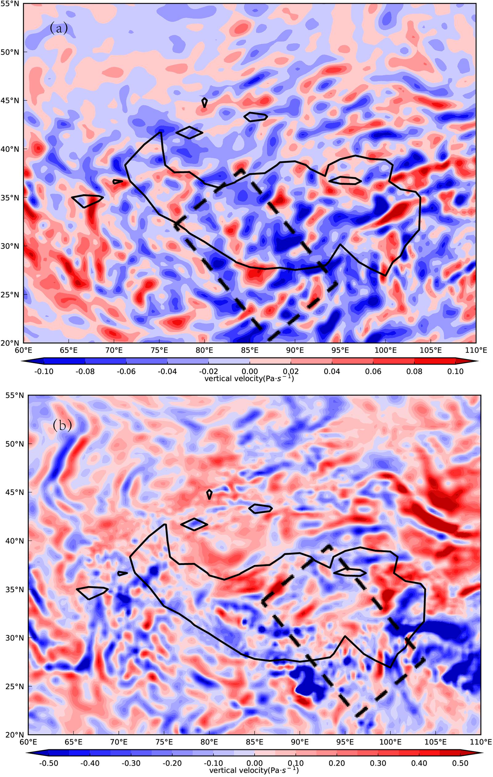
Figure 2. Vertical velocity field (unit: Pa s^–1) at (a) 100 hPa and (b) 400 hPa from ERA5 reanalysis data at 19:00 on 3 May 2014.

Figure 3 shows the longitude–height cross section of vertical velocity, the thermal tropopause and potential vorticity along 28°N taken from ERA5 reanalysis data. According to the World Meteorological Organization (WMO) definition, the thermal tropopause is defined as the lowest level at which the lapse rate decreases to 2°C per km or less, provided also that the average lapse rate between this level and all higher levels within 2 km does not exceed 2°C per km (World Meteorological Organization, 1957). The WMO definition can be applied globally (Liu and Liu, 2016). Usually, the potential vorticity value of 2 PVU (Potential Vorticity Unit, 1 PVU = 10^–6 m² s^–1 K kg^–1) can be defined as the tropopause height over the extratropics (excluding 30°S–30°N; Shapiro, 1980). The figure shows that the height of the tropopause over the Tibetan Plateau is about 16.5 km, which is consistent with the average position of the tropopause over the Tibetan Plateau in summer (Shi et al., 2018). The thermal tropopause height is found to be close to the height of 4 PVU along 28°N, which is the same result as found in a previous study (Shi et al., 2018). Above 85°E–100°E, there is a fluctuating signal, indicating that the vertical velocity is alternately distributed at the center of the positive and negative values in the vertical direction. From 18:00 to 21:00, the gravity wave structure between 90°E and 100°E showed a westward tilt with height. From 19:00 to 21:00, the gravity waves decayed between 90°E and 100°E. From 22:00 to 23:00, the gravity wave shape disappeared. Before 19:00, the wave energy propagated upwards with the group velocity, but the signal was not obvious. After 21:00, the breaking of the gravity waves caused the STE.

FIGURE 3

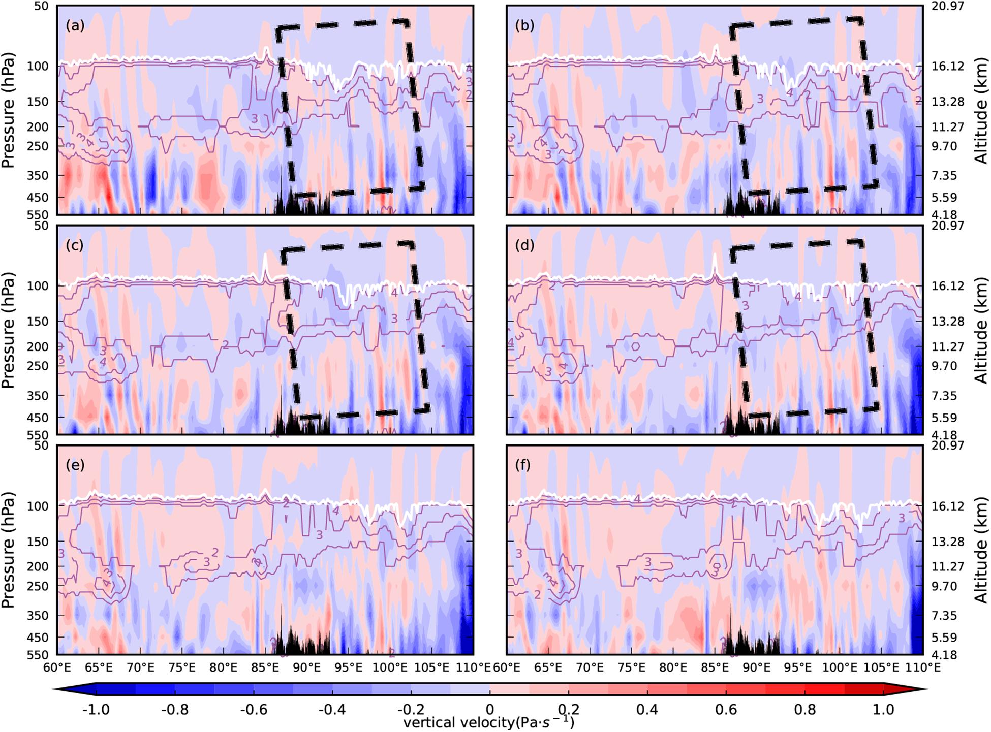
Figure 3. Longitude–height cross section of vertical velocity (unit: Pa s^–1) along 28°N from ERA5 reanalysis data. The solid white lines indicate the thermal tropopause and the solid purple lines indicate potential vorticity (unit: PVU) Times shown are (a) 18:00; (b) 19:00; (c) 20:00; (d) 21:00; (e) 22:00; and (f) 23:00.

From Figures 3a–d, we can estimate that the horizontal wavelengths of the gravity waves range from 200 to 500 km. According to dispersion relations $({\widehat{\mathrm{\omega }}}^2-f^2)=N^2{k}_h^2$, we can derive the horizontal wavenumber k_h, and horizontal wavelength λ_h = 2π/k_h (Bian et al., 2005). Here, N is known buoyancy frequency. $\widehat{\mathrm{\omega }}$ is natural frequency, which can be obtained by $\widehat{\mathrm{\omega }}/\left|f\right|={({\mathrm{\lambda }}_1/{\mathrm{\lambda }}_2)}^{1/2}$. Now, horizontal wind speed vector is [u(z), v(z)], and we suppose A = $\overline{u^{\prime 2}}$, B = $\overline{v^{\prime 2}}$, C = $\overline{u^{\prime }v}$, where u′ and v′ are disturbance variables, and the overline means the average in height. We choose the height from 450 hPa to 50 hPa with obvious waveform. We can then derive ${\mathrm{\lambda }}_{1,2}=\left[A+B\pm \sqrt{{\left(A-B\right)}^2+4C^2}\right]/2$. Based on the theoretical formula λ_z = 2πU/k_h for the vertical wavelength of terrain gravity waves, we can estimate the vertical wavelength of the gravity waves, in which U is the zonal wind speed near the terrain. The calculation results show the theoretical horizontal wavelength is 600 km and the theoretical vertical wavelength is nearly 3.5 km.

Figure 4 shows the time evolution of vertical velocity with longitude over 28°N from ERA5 reanalysis data for the period 18:00–23:00 on 3 May, 2014 at 200 hPa (Figure 4). Between 90°E and 100°E, the vertical velocity shows a westward tilt with time. But from 21:00 to 23:00, the gravity wave shape gradually decayed and disappeared at 200 hPa between 90°E and 100°E. This is consistent with the breaking of the gravity waves.

FIGURE 4

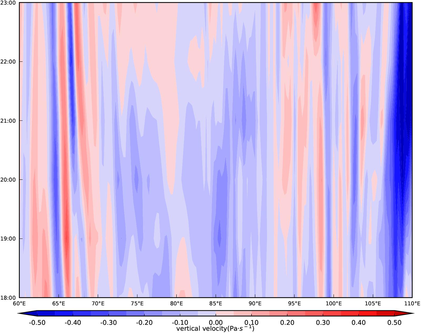
Figure 4. The time evolution of vertical velocity (unit: Pa s^–1) with longitude over 28°N from ERA5 for the period 18:00–23:00 on 3 May, 2014 at 200 hPa.

As terrain-triggered convection can also trigger gravity waves (Hoffmann et al., 2013), is this gravity wave caused by the terrain? In general, atmospheric stratification stability can be characterized by the buoyancy frequency, $N^2=g\frac{dln\overline{\mathrm{\theta }}}{dz}$. When N² > 0, the atmospheric stratification is stable, and it is not easy to generate convective activities. On the other hand, if N² < 0 then convective activities easily occur. Therefore, the buoyancy frequency can be used to diagnose whether the gravity wave event is triggered by topography (Wei et al., 2016).

Figure 5 shows the buoyancy frequency along 28°N from ERA5 reanalysis data on 3 May, 2014, from 19:00 to 23:00. Since the air in the stratosphere is more stable than that in the troposphere, N² gradually increases from the troposphere to the stratosphere. A dense N² contour area appears near 100 hPa, indicating that N² has a large gradient in the UTLS region. At the same time, it can be seen that N² was always positive in the troposphere during the gravity wave process, indicating that the atmosphere in the region was always in a stable stratified state at that time. Thus, it was not easy to produce convection. This shows the gravity wave signal was not induced by deep convection but was generated by the terrain. We notice that there was a low center of buoyancy frequency above 150 hPa between 60°E and 80°E which was consistent with dynamical tropopause (2PV). In addition, there was another low center of buoyancy frequency between 85°E and 95°E at 350–100 hPa, which gradually became smaller with time. This was related to the STE. In the following section, this mass and energy exchange process will be analyzed in detail.

FIGURE 5

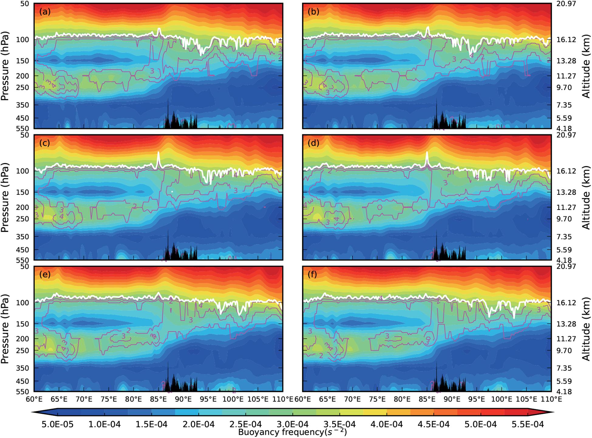
Figure 5. Longitude–height cross section of buoyancy frequency (unit: s^–2) along 28°N from ERA5 reanalysis data on 3 May, 2014. The solid white lines indicate the thermal tropopause and the solid purple lines indicate potential vorticity (unit: PVU). Times shown are (a) 18:00; (b) 19:00; (c) 20:00; (d) 21:00; (e) 22:00; and (f) 23:00.

The Response of Ozone in the UTLS to the Gravity Wave

Figure 6 shows the longitude–height cross section of the ozone mixing ratio along 28°N from the ERA5 reanalysis data on 3 May, 2014. At 18:00, the upper troposphere showed a lower ozone mixing ratio and the lower stratosphere showed a greater ozone mixing ratio. From 550–250 hPa in the gravity wave activity area over 85°E–95°E, the ozone mixing ratio value was relatively low and the ozone isoline protruded toward the upper atmosphere, which was consistent with the terrain. In the UTLS region above 200 hPa, the ozone mixing ratio distribution was relatively even. From 19:00 to 21:00, the tropopause height between 90°E and 100°E is decreased, which was consistent with the decaying of gravity wave. After 21:00, the breaking of gravity wave caused the STE between 90°E and 100°E. The abnormal signal of ozone was gradually generated at 300–100 hPa over 92.5°E–98.5°E, shown in the black box area. The ozone mixing ratio increased and the “ridge” moved downwards. During this period, from 300–150 hPa above 90°E (in the black box area) the high-value ozone area also began to extend downwards, displaying a “tongue” structure. It can be concluded from this that ozone exchange between the lower stratosphere and the upper troposphere led to an increased ozone concentration in the latter. The abnormal ozone distribution in the UTLS region showed a good response to the gravity wave event, mainly because of the ozone exchange in the UTLS that was triggered by the gravity waves breaking.

FIGURE 6

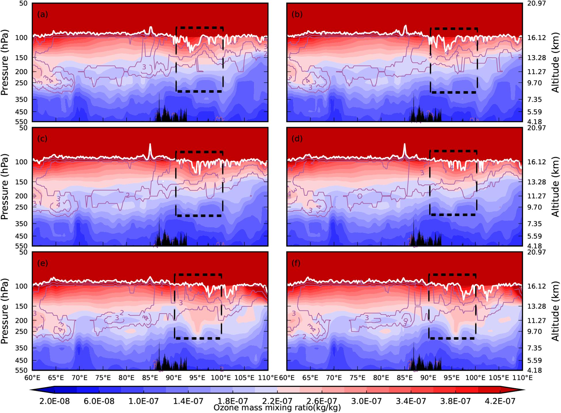
Figure 6. Longitude–height cross section of the ozone mixing ratio (unit: kg/kg) along 28°N from ERA5 reanalysis data on 3 May, 2014. The solid white lines indicate the thermal tropopause and the solid purple lines indicate potential vorticity (unit: PVU). Times shown are (a) 18:00; (b) 19:00; (c) 20:00; (d) 21:00; (e) 22:00; and (f) 23:00.

Figure 7 shows the time evolution of the vertical distribution of potential vorticity (PV) and ozone mixing ratios from ERA5 reanalysis data for the period 18:00–23:00 on 3 May, 2014 above 28°N, averaged between 92.5°E and 98.5°E. The potential vorticity and ozone mixing ratios varied significantly. From 20:00 to 21:00, potential vorticity intrusions extend downwards, as shown in Figure 7a, but the signal is not obvious. These potential vorticity intrusions were followed by injections of stratospheric ozone-enriched air into the upper troposphere from 21:00 to 22:00. High ozone concentrations can be seen at that point in the upper troposphere in Figure 7b. According to an earlier study, there is a correlation between potential vorticity and ozone in the UTLS (Lamarque et al., 1996). In order to investigate this, it is necessary to use the WRF mesoscale model to simulate the variation of potential vorticity.

FIGURE 7

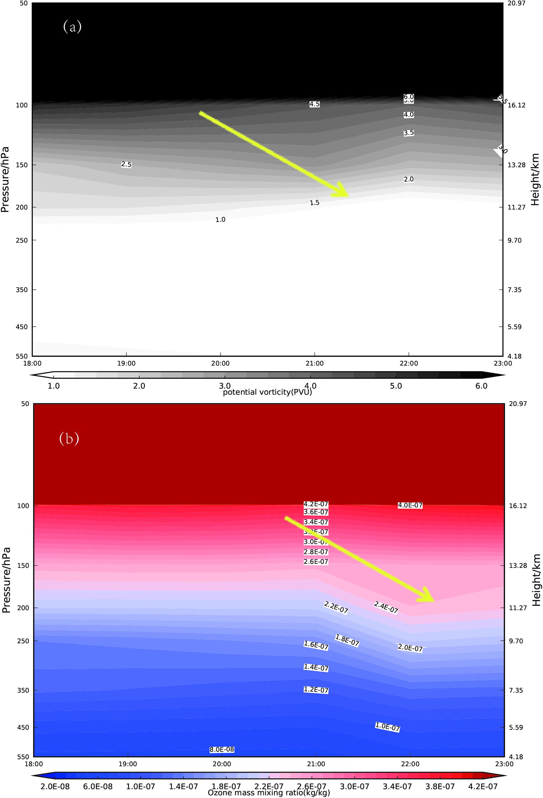
Figure 7. The time evolution of the vertical distribution of (a) potential vorticity (PV) and (b) ozone mixing ratios from ERA5 reanalysis data for the period 18:00–23:00 on 3 May, 2014 above 28°N, averaged between 92.5°E and 98.5°E.

During this whole process, the gravity waves decayed from 19:00 onwards between 90°E and 100°E. From 21:00 to 23:00, the gravity wave shape disappeared and the gravity waves broke. From 21:00, the stratospheric ozone exchange had begun, completing the stratosphere and troposphere mass exchange. However, because ERA5 reanalysis data filter out some small-scale and mesoscale disturbances, the features of gravity waves at these scales cannot be extracted effectively. From Figure 1, we can see that the scale of this gravity wave event is small, hence the necessity to use the mesoscale WRF model in the following analysis.

Analysis of WRF Simulation Results

Although ERA5 reanalysis data have temporal and spatial resolution, they cannot fully describe small-scale and mesoscale fluctuation processes. In order to better describe the spatial structure and time evolution characteristics of gravity waves, and to explore the ozone response to the gravity waves in the UTLS region, the mesoscale WRF model is used to simulate the gravity wave event. Detailed characteristics of the ozone and energy exchange caused by the gravity wave processes are analyzed.

Figure 8 shows the vertical velocity field simulated by the WRF model at 100 hPa and 400 hPa at 19:00 on 3 May 2014. It can be seen from Figure 8a that the area where the gravity waves appeared is 80°E–95°E, 22°N–32°N (within the black box), which is in accordance with Figure 1. From 400 hPa (Figure 8b) to 100 hPa (Figure 8a), the gravity wave structure shows a westward tilt with height. Compared with the vertical velocity obtained from ERA5 reanalysis data (Figure 2), the gravity wave signal obtained by WRF is more obvious, but the gravity wave areas in both figures are the same. It can be seen from Figure 8 that the most obvious area of the waves is 85°E–100°E. The horizontal wavelength of the gravity wave simulated by the WRF model is more obvious compared with that from ERA5 reanalysis data, and is also in accordance with the gravity waves observed in Figure 1. This shows that the WRF model can simulate the basic characteristics of the gravity wave signal.

FIGURE 8

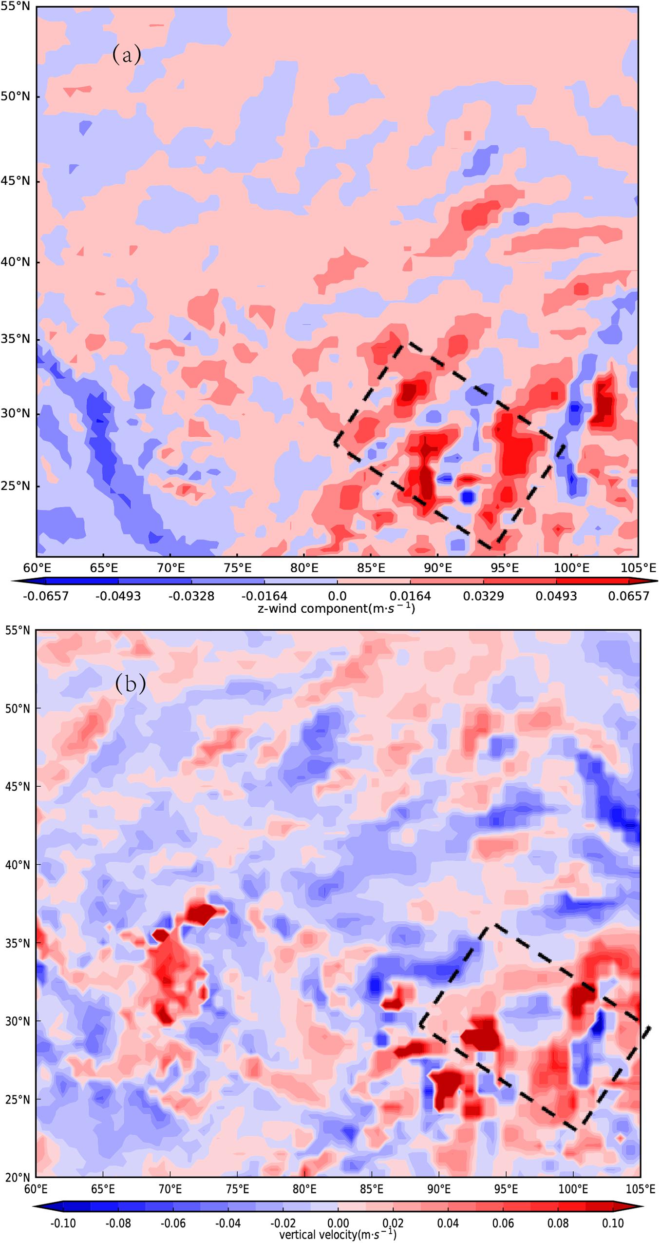
Figure 8. WRF-model simulation of vertical velocity (unit: m s^–1) at (a) 100 hPa and (b) 400 hPa over the Tibetan Plateau at 19:20 on 3 May, 2014.

To show the gravity wave signal more clearly, and to compare the gravity wave signal obtained by WRF with that from ERA5 data, we also present the longitude–height cross section of the vertical velocity along 28°N simulated by WRF (Figure 9). The solid white lines indicate the thermal tropopause and the solid purple lines indicate potential vorticity simulated by WRF It can be seen that the vertical velocity inclined structure given by WRF is basically consistent with the corresponding characteristics of the gravity wave obtained from ERA5 reanalysis data, but the WRF simulation results are clearer. During its progress, the vertical gravity wave train tilted westward between 90°E and 100°E. From 18:20 to 19:20, the waveform signal gradually increased. From 19:20 to 21:20, the gravity waves decayed between 90°E and 100°E and from 21:20 to 23:20, the fluctuation signal became gradually blurred. The above results show that the WRF model can simulate well the spatiotemporal evolution characteristics of the gravity wave signal. Compared with the results obtained from ERA reanalysis data, gravity waves simulated by WRF can be recognized more clearly and the gravity wave processes can be better reflected, especially in the vertical direction.

FIGURE 9

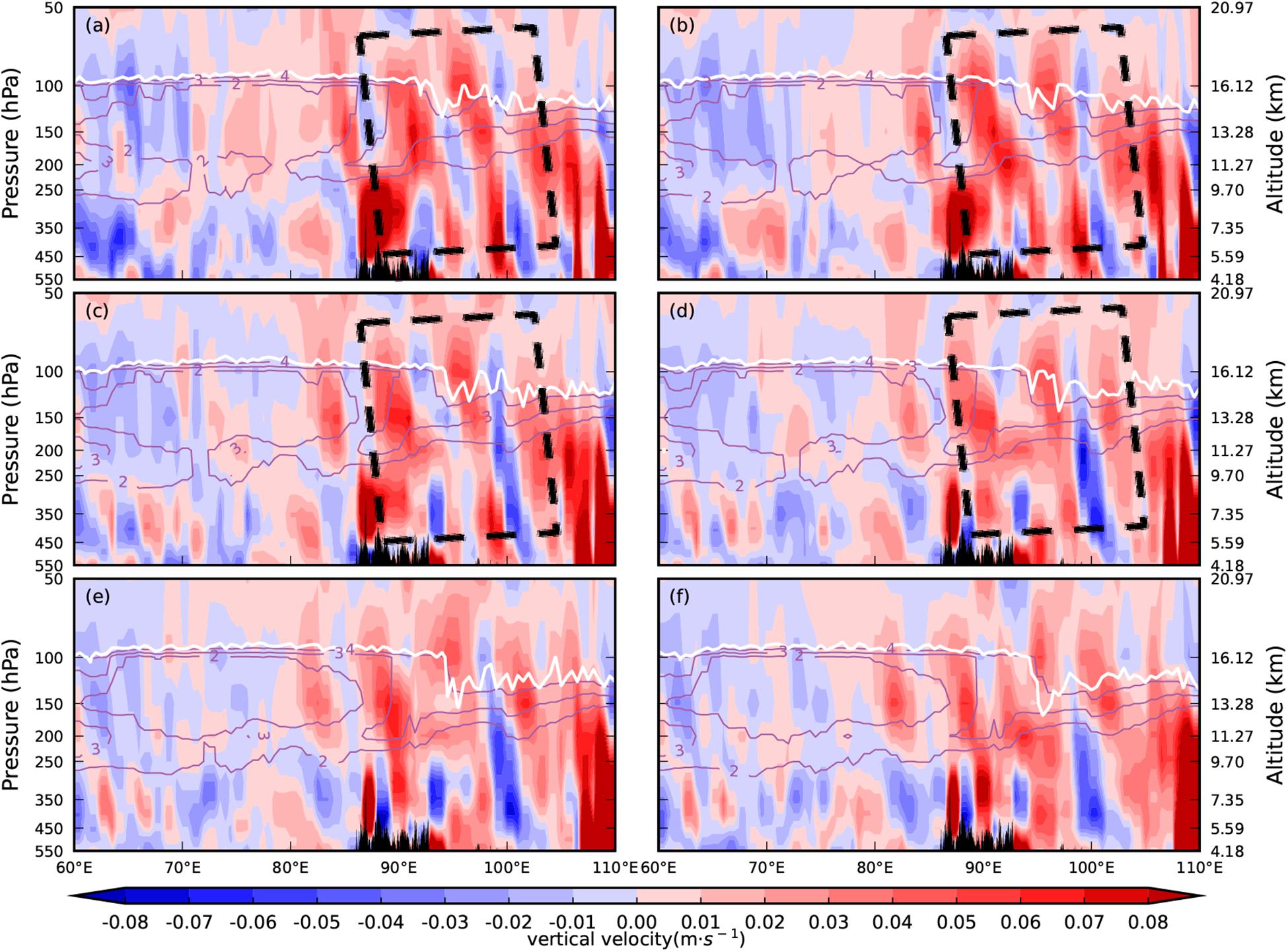
Figure 9. Longitude–height cross section of vertical velocity (unit: m s^–1) along 28°N simulated by WRF. The solid white lines indicate the thermal tropopause and the solid purple lines indicate potential vorticity (unit: PVU). Times shown are (a) 18:20; (b) 19:20; (c) 20:20; (d) 21:20; (e) 22:20; and (f) 23:20.

For comparison, we also give the time evolution of vertical velocity with longitude over 28°N simulated by WRF for the period 18:20–23:20 on 3 May, 2014 at 200 hPa (Figure 10). Between 85°E and 100°E, the vertical velocity shows a westward tilt with time. From 21:20 to 23:20, the gravity wave shape disappeared between 85°E and 100°E, which is consistent with the breaking of the gravity waves. Compared with the result from ERA5 reanalysis data (Figure 4), the gravity wave signals simulated by WRF are clearer.

FIGURE 10

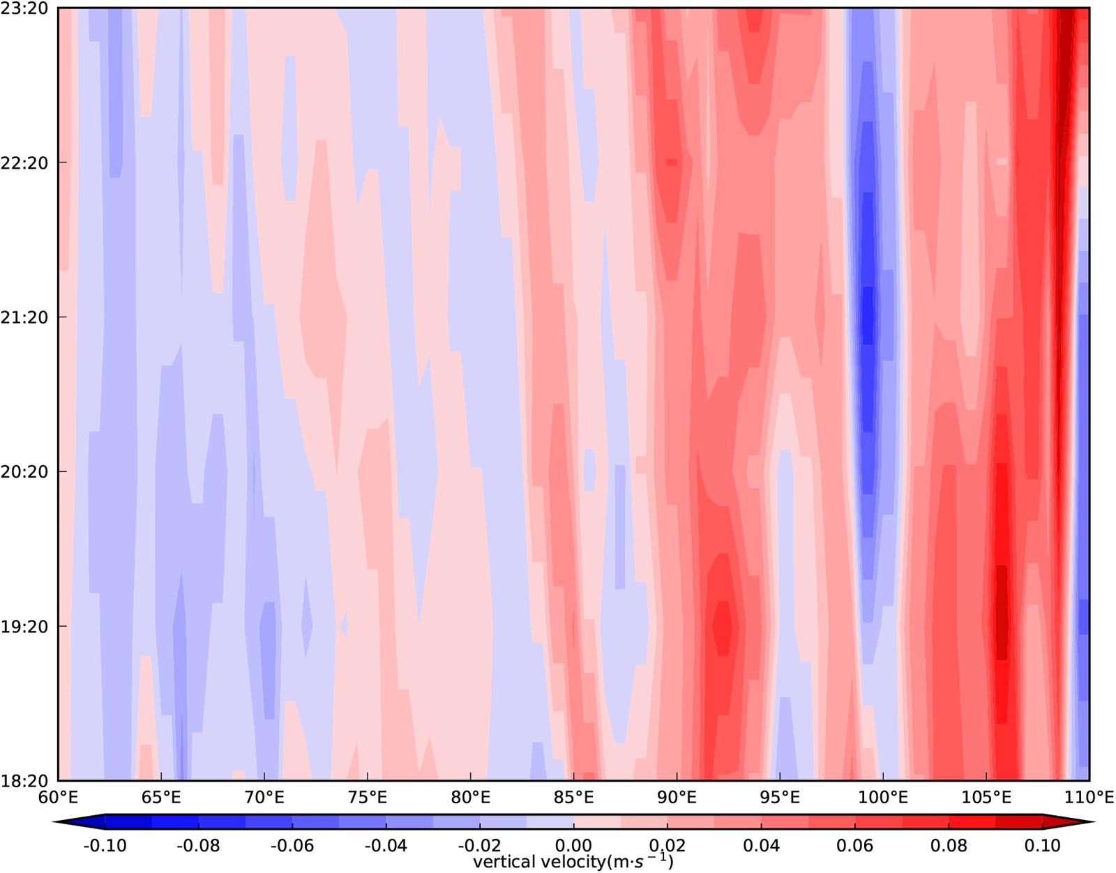
Figure 10. The time evolution of vertical velocity (unit: m s^–1) with longitude over 28°N simulated by WRF for the period 18:20–23:20 on 3 May, 2014 at 200 hPa.

Compared with the ozone mixing ratios shown in Figure 6, WRF simulation (Figure 11) shows little variation with time in the stratosphere. The ozone mixing ratios in the troposphere, however, show some variation. This is because ozone mixing ratios can be better simulated by WRF in the troposphere, whereas results in the stratosphere, the simulated results are not as good. From 21:20 to 23:20, the tropopause height simulated by WRF between 90°E and 100°E decreased, which is consistent with the breaking of the gravity waves. At the same time, between 90°E and 100°E in the upper troposphere (black box area in Figure 6), the ozone mixing ratio increased and the “ridge” moved downwards. The variation characteristics of tropopause height from ERA5 reanalysis data after the breaking of the gravity waves are not as obvious as those simulated by WRF because of ERA5’s limitations in representing some small- and medium-scale disturbance features.

FIGURE 11

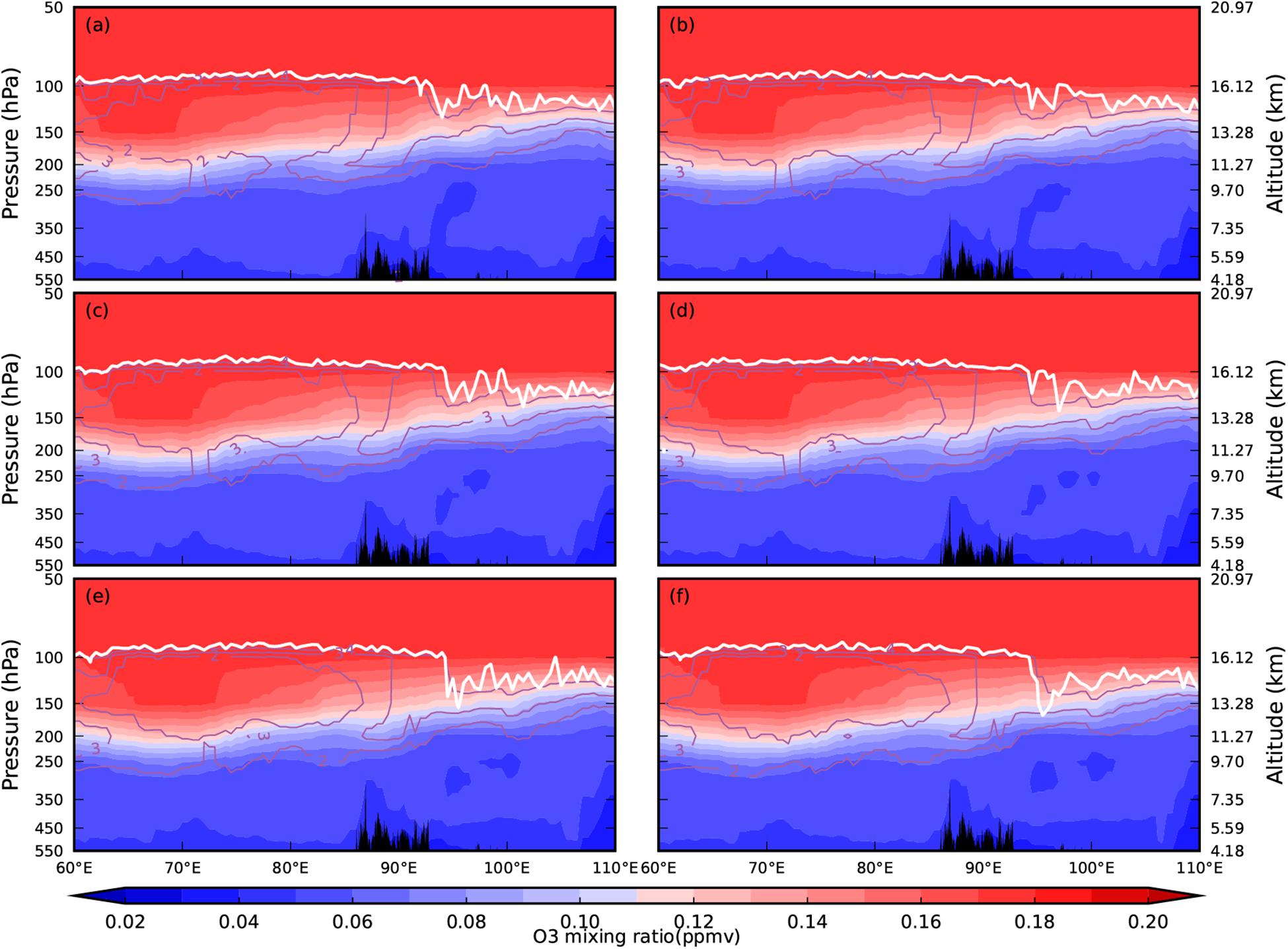
Figure 11. Longitude–height cross section of the ozone mixing ratio (unit: ppmv) along 28°N simulated by WRF on 3 May, 2014. The solid white lines indicate the thermal tropopause and the solid purple lines indicate potential vorticity (unit: PVU). Times shown are (a) 18:20; (b) 19:20; (c) 20:20; (d) 21:20; (e) 22:20; and (f) 23:20.

To further examine the detailed characteristics of ozone variation caused by the upward propagation of gravity waves, the longitude–height cross section of the potential vorticity along 28°N simulated by WRF is shown in Figure 12. Potential vorticity can not only describe weather processes and energy changes, but it can also define the dynamic tropopause height over the extratropics. In general, the potential vorticity in the stratosphere is higher than that in the troposphere. Above 60°E–90°E, after 21:00, the breaking of the gravity waves caused the STE, and the potential vorticity gradually showed even zonal distribution near 250–200 hPa. At the same time, the tropopause height between 90°E and 100°E decreased. Compared with the variation of ozone with time in Figure 6, the decreased tropopause height is consistent with the increased ozone mixing ratio in the upper troposphere.

FIGURE 12

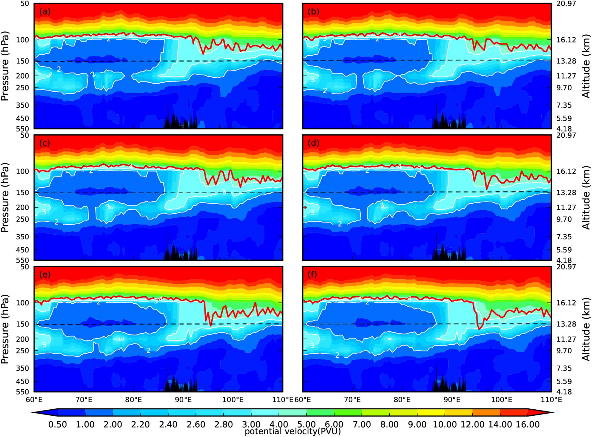
Figure 12. Longitude–height cross section of potential vorticity (unit: PVU) along 28°N simulated by WRF. The red lines indicate the thermal tropopause. The dashed black lines are 150 hPa. Times shown are (a) 18:20; (b) 19:20; (c) 20:20; (d) 21:20; (e) 22:20; and (f) 23:20.

In Figure 13 we compare the time evolution of the vertical distribution of potential vorticity simulated by WRF (Figure 13a) with ozone mixing ratios from ERA5 (Figure 13b, also Figure 7b) for the period 18:00–23:00 on 3 May 2014 above 28°N, averaged between 92.5–98.5°E. Figure 13a shows that, from 20:20 to 21:20, potential vorticity intrusions extended downwards, as in Figure 7a. Accompanying these intrusions, from 21:00 to 22:00, stratospheric ozone-enriched air was injected into the upper troposphere. High ozone concentrations can be seen in the upper troposphere in Figure 13b.

FIGURE 13

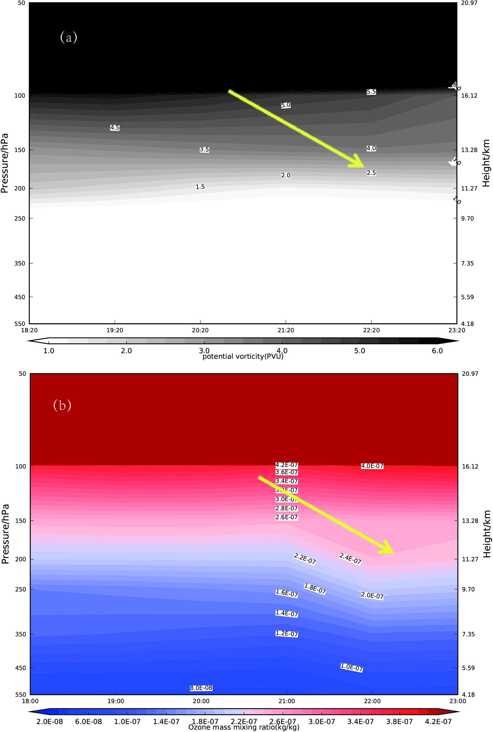
Figure 13. The time evolution of (a) the vertical distribution of potential vorticity (PV) simulated by WRF and (b) ozone mixing ratios from ERA5 (also Figure 7B) for the period 18:00–23:00 on 3 May, 2014 above 28° N, averaged between 92.5°E–98.5°E.

The breaking of gravity waves causes turbulent flow, which will lead to the mixing of momentum and mass. Therefore, the momentum flux $\overline{u^{\prime }{w}^{\prime }}$ caused by turbulent flow will change (Kawatani et al., 2005). Study has shown that the momentum flux $\overline{u^{\prime }{w}^{\prime }}$ is inversely proportional to the potential vorticity vertical flux $\overline{P{V}^{\prime }{w}^{\prime }}$ (Wei et al., 2016). After the breaking of gravity waves, intense energy will be released, the decaying of $\overline{u^{\prime }{w}^{\prime }}$ being the strongest source. Thus, potential vorticity vertical flux $\overline{P{V}^{\prime }{w}^{\prime }}$ increases rapidly. During the process, we know that zones in the UTLS region can respond to the STE process generated by the breaking of gravity waves. In order to diagnose the breaking of gravity waves in the UTLS region, the potential vorticity vertical flux $\overline{P{V}^{\prime }{w}^{\prime }}$ can be used as an indicator for analysis.

In Figure 14, which shows the longitude–height cross section of the potential vorticity vertical flux along 28°N simulated by WRF, we focus on the UTLS area where the ozone obviously varied during the process (black box area, 250–125 hPa, 92.5°E–98.5°E). The potential vorticity vertical flux varied significantly in this area, as did the potential vorticity. Based on Figure 14 and Figure 6, we can calculate the average potential vorticity vertical flux $\overline{P{\text{V}}^{\prime }{\text{w}}^{\prime }}$ over 250–125 hPa, between 92.5°E and 98.5°E (black box area in Figure 14), and the average ozone mixing ratio in the same area (shown in Figure 15).

FIGURE 14

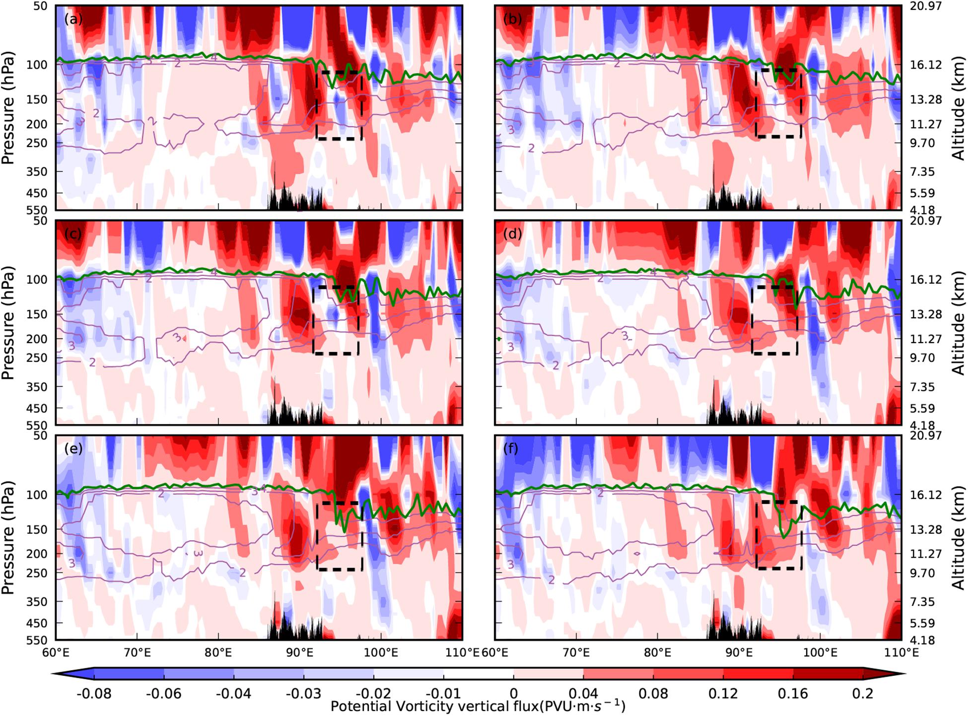
Figure 14. Longitude–height cross section of the potential vorticity vertical flux (unit: PVU⋅m s−¹) along 28°N simulated by WRF. The solid green lines indicate the thermal tropopause and the solid purple lines indicate potential vorticity (unit: PVU). Times shown are (a) 18:20; (b) 19:20; (c) 20:20; (d) 21:20; (e) 22:20; and (f) 23:20.

FIGURE 15

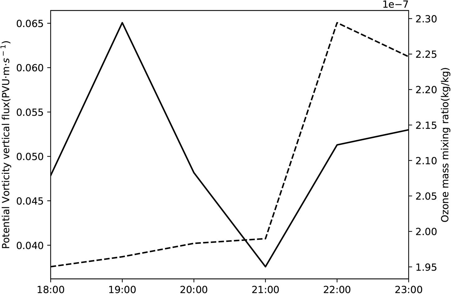
Figure 15. Time variation of the average potential vorticity vertical flux $\overline{P{\mathrm{V}}^{\prime }{\mathrm{w}}^{\prime }}$ (averaged over the 250–125 hPa, 92.5°E–98.5°E area) simulated by WRF (solid line) and the average ozone mixing ratio from ERA5 reanalysis data (dashed line) from 18:00 on 3 May, 2014 to 00:00 on 4 May, 2014.

Figure 15 shows that there was a response in the ozone mixing ratio to the breaking of the gravity waves in this area. From 19:00 to 21:00, with the decaying of the gravity waves, the $\overline{P{V}^{\prime }{w}^{\prime }}$ and the ozone mixing ratio showed little variation. After 21:00, the breaking of the gravity waves caused the STE. Potential vorticity vertical flux $\overline{P{V}^{\prime }{w}^{\prime }}$ increased rapidly Meanwhile, during the breaking of the gravity waves, the STE occrred. Air with greater ozone concentration from the stratosphere was injected into the UTLS, leading to rapidly increased ozone concentration in this area (black box area in Figure 6). The ozone mixing ratio reached its maximum value at 22:00. The ozone variation in the UTLS over the Tibetan Plateau shows a very good response to this gravity wave process.

Conclusion and Discussion

In this paper, ERA5 reanalysis data and the WRF mesoscale model were used to analyze a topographic gravity wave event that occurred over the Tibetan Plateau from 18:00 on 4 May, 2014 to 00:00 on May 4, 2014. The response of ozone to gravity wave processes in the UTLS region was obtained. The results are as follows:

(1) Although ERA5 reanalysis data have temporal and spatial resolution, they cannot fully describe small-scale and mesoscale fluctuation processes. It is necessary therefore to use the mesoscale WRF model to simulate small-scale gravity wave events.

(2) As shown via comparison and simulation analysis, the gravity wave structure between 90°E and 100°E shows a westward tilt with height. From 19:00 to 21:00 the gravity wave decayed. From 22:00 to 23:00, the gravity wave shape gradually blurred.

(3) There was a response of the ozone mixing ratio in the UTLS over the Tibetan Plateau to the breaking of gravity waves. After 21:00, the breaking of the gravity waves caused the STE. Ozone-enriched air from the stratosphere was injected into the upper troposphere, leading to rapidly increased ozone concentration there.

Data Availability Statement

The datasets ECMWF reanalysis 5 (ERA5) from the European Center (ECMWF) for this study can be found in the https://cds.climate.copernicus.eu/#!/home.

Author Contributions

SC, ZS, and YZ designed the experiments. SC and YZ performed the experiments. WS and ZL analyzed the data. SC and ZS wrote the manuscript. All authors contributed to the article and approved the submitted version.

Funding

This work was supported by the National Natural Science Foundation of China (Grant Nos. 41875045 and 41775039), the National Key R&D Program of China (Grant No. 2018YFA0605604), and the project of Enhancing School with Innovation of Guangdong Ocean University (Grant No. 4230419053).

Conflict of Interest

The authors declare that the research was conducted in the absence of any commercial or financial relationships that could be construed as a potential conflict of interest.

Acknowledgments

We thank Profs. Jianjun Xu and Feng Xu from Guangdong Ocean University for providing the WRF (WRF-ARW) v4.0.1 model.

References

Bai, Z., Bian, J., Chen, H., and Chen, L. (2017). Inertial gravity wave parameters for the lower stratosphere from radiosonde data over China. Sci. China Earth Sci. 60, 328–340. doi: 10.1007/s11430-016-5067-y

CrossRef Full Text | Google Scholar

Bian, J., Chen, H., and Lu, D. (2005). Statistics of gravity waves in the lower stratosphere over Beijing based on high vertical resolution radiosonde. Sci. China Ser. D Earth Sci. 48, 1548–1558.

Google Scholar

Bian, J., Li, D., Bai, Z., Li, Q., Lyu, D., and Zhou, X. (2020). Transport of Asian surface pollutants to the global stratosphere from the Tibetan Plateau region during the Asian summer monsoon. Natl. Sci. Rev. 7, 516–533.

Google Scholar

Bian, J., Yan, R., Chen, H., Lü, D., and Massie, S. T. (2011). Formation of the summertime ozone valley over the Tibetan Plateau: the Asian summer monsoon and air column variations. Adv. Atmos. Sci. 28, 1318–1325. doi: 10.1007/s00376-011-0174-9

CrossRef Full Text | Google Scholar

Carslaw, K., Wirth, M., Tsias, A., Luo, B., Dörnbrack, A., Leutbecher, M., et al. (1998). Increased stratospheric ozone depletion due to mountain-induced atmospheric waves. Nature 391, 675–678. doi: 10.1038/35589

CrossRef Full Text | Google Scholar

Chang, S., Sheng, Z., Du, H., Ge, W., and Zhang, W. (2020). A channel selection method for hyperspectral atmospheric infrared sounders based on layering. Atmos. Meas. Tech. 13, 629–644. doi: 10.5194/amt-13-629-2020

CrossRef Full Text | Google Scholar

Chen, D., Chen, Z., and Lü, D. (2012). Simulation of the stratospheric gravity waves generated by the Typhoon Matsa in 2005. Sci. China Earth Sci. 55, 602–610. doi: 10.1007/s11430-011-4303-1

CrossRef Full Text | Google Scholar

Chen, D., Chen, Z., and Lü, D. (2013). Spatiotemporal spectrum and momentum flux of the stratospheric gravity waves generated by a typhoon. Sci. China Earth Sci. 56, 54–62. doi: 10.1007/s11430-012-4502-4

CrossRef Full Text | Google Scholar

Crutzen, P. J. (1970). The influence of nitrogen oxides on the atmospheric ozone content. Q. J. R. Meteorol. Soc. 96, 320–325. doi: 10.1002/qj.49709640815

CrossRef Full Text | Google Scholar

Dudhia, J. (1989). Numerical study of convection observed during the winter monsoon experiment using a mesoscale two-dimensional model. J. Atmos. Sci. 46, 3077–3107. doi: 10.1175/1520-0469(1989)046<3077:nsocod>2.0.co;2

CrossRef Full Text | Google Scholar

Farman, J. C., Gardiner, B. G., and Shanklin, J. D. (1985). Large losses of total ozone in Antarctica reveal seasonal ClO x/NO x interaction. Nature 315, 207–210. doi: 10.1038/315207a0

CrossRef Full Text | Google Scholar

Fetzer, E. J., and Gille, J. C. (1994). Gravity wave variance in LIMS temperatures. Part I: variability and comparison with background winds. J. Atmos. Sci. 51, 2461–2483. doi: 10.1175/1520-0469(1994)051<2461:gwvilt>2.0.co;2

CrossRef Full Text | Google Scholar

Guo, D., Xu, J., Su, Y., Shi, C., Liu, Y., and Li, W. (2017). Comparison of vertical structure and formation mechanism of summer ozone valley over the Tibetan Plateau and North America. Trans. Atmos. Sci. 40, 412–417.

Google Scholar

He, Y., Sheng, Z., and He, M. (2020). Spectral analysis of gravity waves from near space high-resolution balloon data in Northwest China. Atmosphere 11:133. doi: 10.3390/atmos11020133

CrossRef Full Text | Google Scholar

Hoffmann, L., Xue, X., and Alexander, M. (2013). A global view of stratospheric gravity wave hotspots located with Atmospheric Infrared Sounder observations. J. Geophys. Res. Atmos. 118, 416–434. doi: 10.1029/2012JD018658

CrossRef Full Text | Google Scholar

Holton, J. R. (1983). The influence of gravity wave breaking on the general circulation of the middle atmosphere. J. Atmos. Sci. 40, 2497–2507. doi: 10.1175/1520-0469(1983)040<2497:tiogwb>2.0.co;2

CrossRef Full Text | Google Scholar

Hong, S.-Y., Dudhia, J., and Chen, S.-H. (2004). A revised approach to ice microphysical processes for the bulk parameterization of clouds and precipitation. Month. Weather Rev. 132, 103–120. doi: 10.1175/1520-0493(2004)132<0103:aratim>2.0.co;2

CrossRef Full Text | Google Scholar

Hong, S.-Y., Noh, Y., and Dudhia, J. (2006). A new vertical diffusion package with an explicit treatment of entrainment processes. Month. Weather Rev. 134, 2318–2341. doi: 10.1175/mwr3199.1

CrossRef Full Text | Google Scholar

Kain, J. S., and Fritsch, J. M. (1990). A one-dimensional entraining/detraining plume model and its application in convective parameterization. J. Atmos. Sci. 47, 2784–2802. doi: 10.1175/1520-0469(1990)047<2784:aodepm>2.0.co;2

CrossRef Full Text | Google Scholar

Kawatani, Y., Tsuji, K., and Takahashi, M. (2005). Zonally non-uniform distribution of equatorial gravity waves in an atmospheric general circulation model. Geophys. Res. Lett. 32, 308–324.

Google Scholar

Lamarque, J. F., Langford, A. O., and Proffitt, M. H. (1996). Cross-tropopause mixing of ozone through gravity wave breaking: observation and modeling. J. Geophys. Res. Atmos. 101, 22969–22976.

Google Scholar

Liu, N., and Liu, C. (2016). Global distribution of deep convection reaching tropopause in 1 year GPM observations. J. Geophys. Res. Atmos. 121, 3824–3842. doi: 10.1002/2015jd024430

CrossRef Full Text | Google Scholar

Mai, Y., Sheng, Z., Shi, H., Liao, Q., and Zhang, W. (2020). Spatiotemporal distribution of atmospheric ducts in Alaska and its relationship with the Arctic Vortex. Int. J. Antennas Propag. 2020, 1–13. doi: 10.1155/2020/9673289

CrossRef Full Text | Google Scholar

Miller, S. D., Straka, W. C., Yue, J., Smith, S. M., Alexander, M. J., Hoffmann, L., et al. (2015). Upper atmospheric gravity wave details revealed in nightglow satellite imagery. Proc. Natl. Acad. Sci. U.S.A. 112, E6728–E6735.

Google Scholar

Miyazaki, K., Watanabe, S., Kawatani, Y., Tomikawa, Y., Takahashi, M., and Sato, K. (2010). Transport and mixing in the extratropical tropopause region in a high-vertical-resolution GCM. Part I: potential vorticity and heat budget analysis. J. Atmos. Sci. 67, 1293–1314. doi: 10.1175/2009jas3221.1

CrossRef Full Text | Google Scholar

Mlawer, E. J., Taubman, S. J., Brown, P. D., Iacono, M. J., and Clough, S. A. (1997). Radiative transfer for inhomogeneous atmospheres: RRTM, a validated correlated-k model for the longwave. J. Geophys. Res. Atmos. 102, 16663–16682. doi: 10.1029/97jd00237

CrossRef Full Text | Google Scholar

Molina, M. J., and Rowland, F. S. (1974). Stratospheric sink for chlorofluoromethanes: chlorine atom-catalysed destruction of ozone. Nature 249, 810–812. doi: 10.1038/249810a0

CrossRef Full Text | Google Scholar

Pan, L. L., Bowman, K. P., Atlas, E. L., Wofsy, S. C., Zhang, F., Bresch, J. F., et al. (2010). The stratosphere-troposphere analyses of regional transport 2008 experiment. Bull. Am. Meteorol. Soc. 91, 327–342. doi: 10.1175/2009bams2865.1

CrossRef Full Text | Google Scholar

Shapiro, M. (1980). Turbulent mixing within tropopause folds as a mechanism for the exchange of chemical constituents between the stratosphere and troposphere. J. Atmos. Sci. 37, 994–1004. doi: 10.1175/1520-0469(1980)037<0994:tmwtfa>2.0.co;2

CrossRef Full Text | Google Scholar

Sheng, Z., Zhou, L., and He, Y. (2020). Retrieval and analysis of the strongest mixed layer in the troposphere. Atmosphere 11:264. doi: 10.3390/atmos11030264

CrossRef Full Text | Google Scholar

Shi, C., Chang, S., Guo, D., Xu, J., and Zhang, C. (2018). Exploring the relationship between the cloud-top and tropopause height in boreal summer over the Tibetan Plateau and its adjacent region. Atmos. Ocean. Sci. Lett. 11, 173–179. doi: 10.1080/16742834.2018.1438738

CrossRef Full Text | Google Scholar

Shi, C., Xu, T., Guo, D., and Pan, Z. (2017a). Modulating effects of planetary wave 3 on a stratospheric sudden warming event in 2005. J. Atmos. Sci. 74, 1549–1559. doi: 10.1175/jas-d-16-0065.1

CrossRef Full Text | Google Scholar

Shi, C., Zhang, C., and Guo, D. (2017b). Comparison of electrochemical concentration cell ozonesonde and microwave limb sounder satellite remote sensing ozone profiles for the center of the South Asian High. Remote Sens. 9:1012. doi: 10.3390/rs9101012

CrossRef Full Text | Google Scholar

Spang, R., Hoffmann, L., Müller, R., Grooß, J.-U., Tritscher, I., Höpfner, M., et al. (2018). A climatology of polar stratospheric cloud composition between 2002 and 2012 based on MIPAS/Envisat observations. Atmos. Chem. Phys. 18, 5089–5113. doi: 10.5194/acp-18-5089-2018

CrossRef Full Text | Google Scholar

Tian, W., Chipperfield, M., and Huang, Q. (2008). Effects of the Tibetan Plateau on total column ozone distribution. Tellus B Chem. Phys. Meteorol. 60, 622–635. doi: 10.1111/j.1600-0889.2008.00338.x

CrossRef Full Text | Google Scholar

Wang, Y., Wang, H., and Wang, W. (2020). A stratospheric intrusion-influenced ozone pollution episode associated with an intense horizontal-trough event. Atmosphere 11:164. doi: 10.3390/atmos11020164

CrossRef Full Text | Google Scholar

Wei, D., Tian, W., Chen, Z., Zhang, J., Xu, P., Huang, Q., et al. (2016). Upward transport of air mass during a generation of orographic waves in the UTLS over the Tibetan Plateau. Chin. J. Geophys. 59, 791–802.

Google Scholar

World Meteorological Organization [WMO] (1957). Meteorology—A three-dimensional science: second session of the commission for aerology. WMO Bull. 4, 134–138.

Google Scholar

Xia, Y., Huang, Y., and Hu, Y. (2018). On the climate impacts of upper tropospheric and lower stratospheric ozone. J. Geophys. Res. Atmos. 123, 730–739. doi: 10.1002/2017jd027398

CrossRef Full Text | Google Scholar

Zhang, J., Tian, W., Xie, F., Tian, H., Luo, J., Zhang, J., et al. (2014). Climate warming and decreasing total column ozone over the Tibetan Plateau during winter and spring. Tellus Ser. B Chem. Phys. Meteorol. 66, 1–12.

Google Scholar

Zhou, X., Li, W., Chen, L., and Liu, Y. (2004). Study of ozone change over Tibetan Plateau. Acta Meteorol. Sin. 62, 513–527.

Google Scholar

Zhou, X., and Luo, C. (1994). Ozone valley over Tibetan Plateau. J. Meteorol. Res. 8, 505–506.

Google Scholar