Insights Into Microseism Sources by Array and Machine Learning Techniques: Ionian and Tyrrhenian Sea Case of Study

In this work, we investigated the microseism recorded by a network of broadband seismic stations along the coastline of Eastern Sicily. Microseism is the most continuous and ubiquitous seismic signal on Earth and is mostly generated by the ocean–solid earth interaction. On the basis of spectral content, it is possible to distinguish three types of microseism: primary, secondary, and short-period secondary microseism (SPSM). We showed how most of the microseism energy recorded in Eastern Sicily is contained in the secondary and SPSM bands. This energy exhibits strong seasonal patterns, with maxima during the winters. By applying array techniques, we observed how the SPSM sources are located in areas of extended shallow water depth: the Catania Gulf and a part of the Northern Sicily coastlines. Finally, by using the significant wave height data recorded by two buoys installed in the Ionian and Tyrrhenian Seas, we developed an innovative method, selected among up-to-date machine learning techniques (MLTs), able to reconstruct the time series of sea wave parameters from microseism recorded in the three microseism period bands by distinct seismic stations. In particular, the developed model, based on random forest regression, allowed estimating the significant wave height with a low average error (∼0.14–0.18 m). The regression analysis suggests that the closer the seismic station to the sea, the more information concerning the sea state are contained in the recorded microseism. This is particularly important for the future development of an experimental monitoring system of the sea state conditions based on microseism recordings.

Introduction

Microseism is the most continuous and ubiquitous seismic signal on Earth and is mostly generated by the ocean–solid earth interaction (Tanimoto et al., 2015). On the basis of its source mechanism and spectral content, it is classified as: primary microseism (hereafter referred to as PM), secondary microseism (SM), and short-period secondary microseism (SPSM) (Haubrich and McCamy, 1969). Concerning PM, it shares the same spectral content as the ocean waves (period band 13–20 s) and its source is associated with the energy transfer of ocean waves breaking/shoaling against the shoreline (Hasselmann, 1963; Ardhuin et al., 2015). As for SM, it is likely to be generated by interactions between waves of the same frequency traveling in opposite directions, has roughly twice the frequency of ocean waves (period band 5–10 s), and generally shows a higher amplitude than does PM (Longuet-Higgins, 1950; Oliver and Page, 1963; Ardhuin et al., 2012, 2015). Finally, SPSM is characterized by a period shorter than 5 s and is generated by local nearshore wave–wave interaction (Bromirski et al., 2005).

Because of its source mechanism, microseism has been used to make inferences on climate changes (e.g., Grevemeyer et al., 2000; Aster et al., 2008; Stutzmann et al., 2009). For instance, Grevemeyer et al. (2000) analyzed a 40-year-long record of wintertime microseism and observed an increase in the number of monthly days with strong microseism activity, hence inferring an increase over time in surface air temperatures and storminess of the northeast Atlantic Ocean.

Microseism amplitudes show strong seasonal modulation. Indeed, at temperate latitudes, microseism shows periodicity, with maxima during the winter seasons, when the oceans are stormier, and minima during the summers (Aster et al., 2008). This modulation is different along the coastlines of the Glacial Arctic Sea and the Southern Ocean where, during the winters, because of the sea ice, the oceanic waves cannot efficiently excite seismic energy (Aster et al., 2008; Stutzmann et al., 2009; Tsai and McNamara, 2011; Cannata et al., 2019).

Concerning the source location, microseism signals are non-impulsive, and the sources are generally diffuse and variable in time (e.g., Bromirski et al., 2013). Hence, the classical location algorithms, used in earthquake seismology and based on the picking of the different seismic phases, cannot be applied to locate microseism sources. Array processing techniques can overcome the above-mentioned difficulties and provide information on the microseism source areas that generally coincide with coastal regions and/or oceanic storm systems (e.g., Chevrot et al., 2007; Juretzek and Hadziioannou, 2017; Pratt et al., 2017; Lepore and Grad, 2018).

The link between microseism amplitudes and the ocean wave height has been empirically explored by several authors (e.g., Bromirski et al., 1999; Bromirski and Duennebier, 2002; Ardhuin et al., 2012; Ferretti et al., 2013, 2018). For instance, Bromirski et al. (1999) determined site-specific seismic-to-wave transfer functions in the San Francisco Bay area (California). Ferretti et al. (2013, 2018) found empirical relations to predict the significant wave height along the Ligurian coast (Italy). In addition, other authors have derived physics-based models of the generation of the different kinds of microseism from the sea state (e.g., Gualtieri et al., 2013; Ardhuin et al., 2015; Gualtieri et al., 2019).

Microseism investigations and, more generally, seismological studies are currently undergoing a rapid increase in dataset volumes (e.g., Kong et al., 2018; Jiao and Alavi, 2019). For this reason, nowadays, applications of machine learning techniques (hereafter referred to as MLTs) on seismological data are increasing in number day by day. Such techniques are used to extract information directly from data using well-defined optimization rules and help unravel hidden relationships between distinct parameters, as well as to build predictive models (e.g., Kuhn and Johnson, 2013; Kong et al., 2018). Examples of the applications of MLTs to seismology include earthquake detection and phase picking (e.g., Wiszniowski et al., 2014) and earthquake early warning (e.g., Kong et al., 2016).

In spite of the availability of seismic and buoy data in the Ionian and Tyrrhenian Seas and coastlines, the link between sea waves and microseism has never been explored in such areas. Furthermore, although the spectral features of the microseism recorded in this area have been studied (e.g., De Caro et al., 2014), the locations of its sources have never been constrained. In this work, we will study the microseism recorded along the coastline of Eastern Sicily in terms of spectral content, amplitude seasonal pattern, and source location. In addition, we will present a novel algorithm, based on up-to-date MLTs, able to reconstruct significant wave height time series in points located in both the Ionian and the Tyrrhenian Seas from the microseism recordings.

Materials and Methods

Data

In order to investigate microseism, seismic signals recorded from 2010 to 2014 by the vertical component of six stations, belonging to the seismic permanent network run by Istituto Nazionale di Geofisica e Vulcanologia, Osservatorio Etneo – Sezione di Catania (INGV-OE), were used (Figure 1a). These stations are equipped with broadband three-component Trillium 40-s seismometers (Nanometrics^TM) recording at a sampling rate of 100 Hz.

FIGURE 1

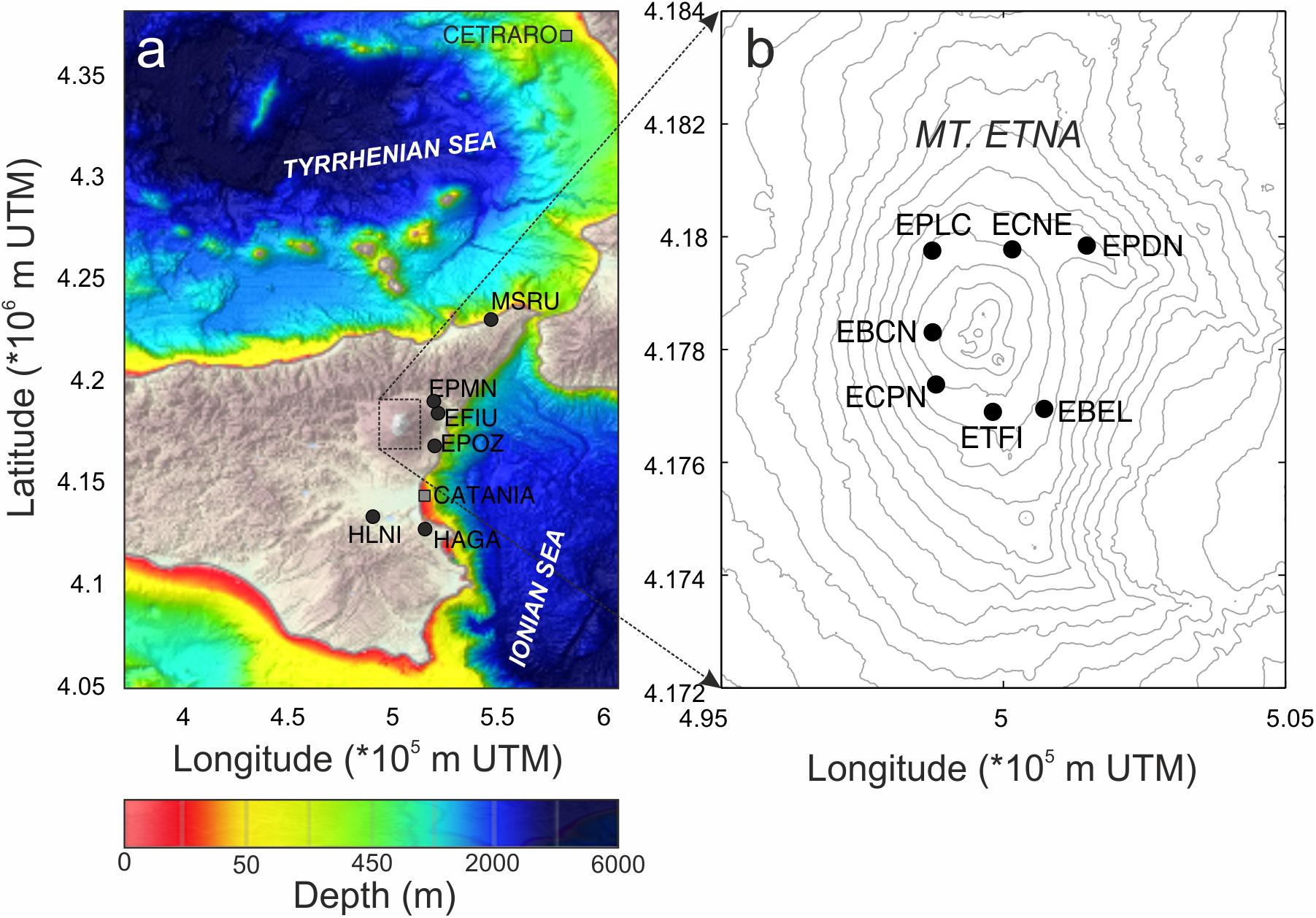
Figure 1. (a) Bathymetric and topographic map (EMODnet Bathymetry Consortium, 2018), with the locations of the seismic stations (black dots), used to perform spectral and amplitude analysis of the microseism and to investigate its relationship with significant wave height, recorded by Catania and Cetraro buoy stations (gray squares). (b) Digital elevation model of Mt. Etna, with the locations of the seismic stations (black dots), used to perform array analysis.

Moreover, to carry out array analysis, seismic signals recorded in January 2010–February 2012 by the vertical component of the seven stations (equipped with the same sensors as above), composing the summit ring of the Mt. Etna permanent seismic network, were used (Figure 1b). These stations were chosen because of: (i) the availability of continuously recorded data during the time interval 2010–beginning of 2012 (in February–March 2012, EBEL and ETFI stations were destroyed by lava flows); (ii) the ring-shaped geometry; and (iii) the distance from the coastline (and then from the prospective closest microseism sources associated with the nearshore wave–coast or wave–wave interaction).

Finally, to make quantitative comparisons between the microseism and wave height time series in the Ionian and the Tyrrhenian Seas, significant wave height data, recorded from 2010 to 2014 with a 30-min sampling step by two stations (Catania and Cetraro; see Figure 1A) belonging to the Italian Data Buoy Network, managed by Istituto Superiore per la Protezione e la Ricerca Ambientale (ISPRA), were used (Bencivenga et al., 2012; Figure 2). The significant wave height is defined as:

FIGURE 2

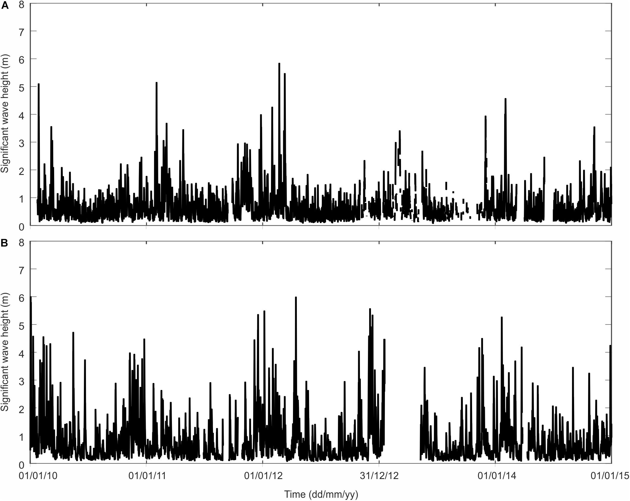
Figure 2. Significant wave height time series recorded by the Catania (A) and Cetraro (B) buoys.

$$H_s=4\sqrt{M_0}(1)$$

where M₀ is the 0-moment of the auto-spectral correlation of the Fourier transformations of the buoy displacements in the frequency/time domain (Steele and Mettlach, 1993):

$$M_0=\sum _{f_l}^{f_u}(S(f)d(f))(2)$$

where the sum of the spectral density S(f) is over all frequency bands, from the lowest frequency f_l to the highest frequency f_u of the non-directional wave spectrum (calculated only for the elevation of the sea surface), and d(f) is the bandwidth of each band.

Spectral and Amplitude Analysis

The spectral content of the seismic data, recorded by the vertical component of the six seismic stations shown in Figure 1a, was analyzed as follows: (i) spectra over non-overlapping 81.92-s-long sliding windows were computed; (ii) to obtain daily spectra (that is, spectra representing the frequency features of the signal acquired during a given day), all the spectra computed in (i) falling on the same day were averaged by Welch’s segment averaging estimator (Welch, 1967); (iii) all the daily spectra were collected and visualized as spectrograms, which are 3D plots with time on the x-axis, frequency on the y-axis, and power spectral density (PSD) indicated by a color scale (Figure 3A).

FIGURE 3

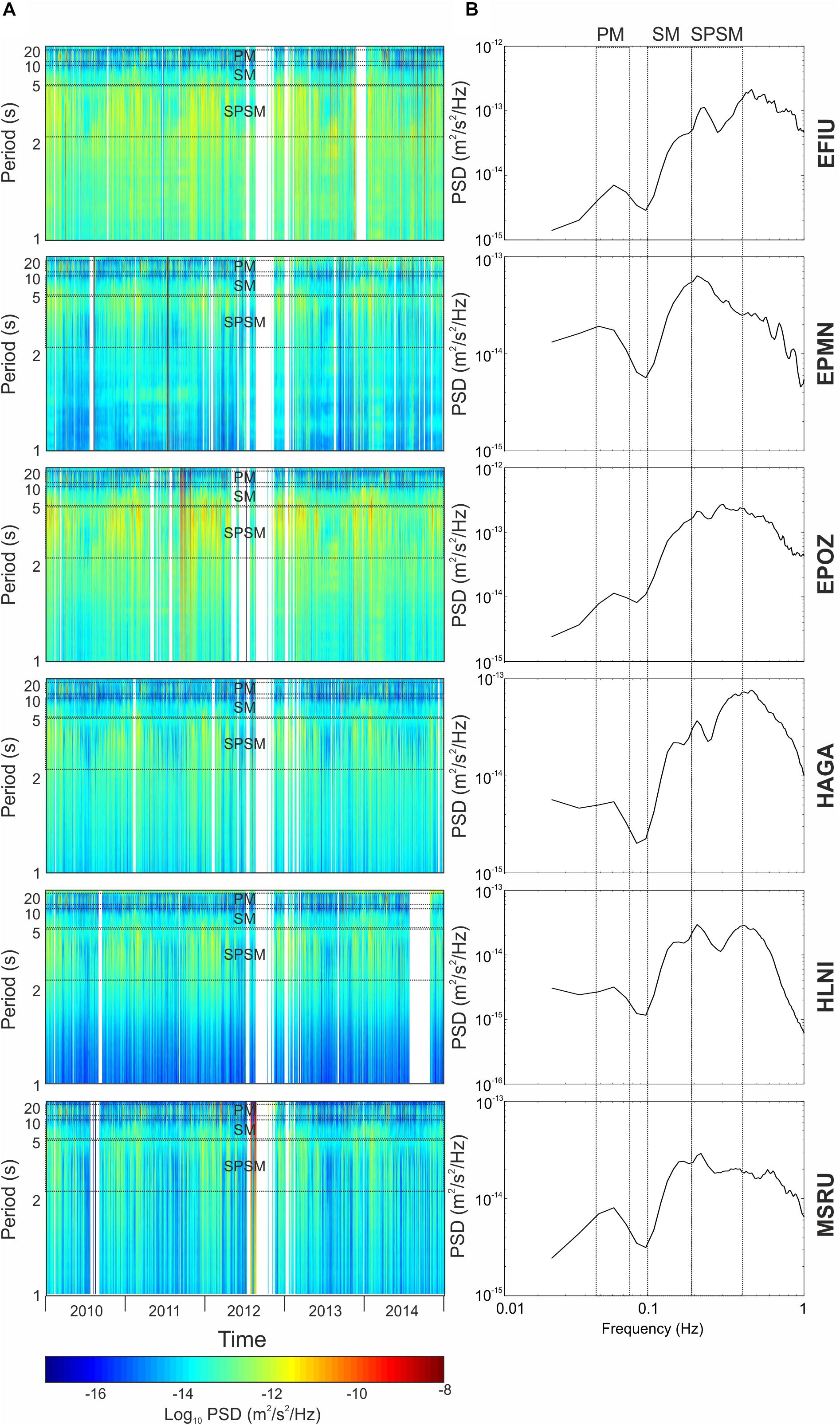
Figure 3. (A) Spectrograms of the seismic signal recorded by the vertical component of the six considered stations. (B) Median spectra of the seismic signal recorded by the vertical component of the six considered stations. The acronyms PM, SM, and SPSM indicate primary microseism, secondary microseism, and short-period secondary microseism, respectively.

Besides, to obtain information on the spectral features of the seismic signals recorded by the different stations during the whole investigated period, all the daily spectra composing the spectrograms were averaged. Hence, spectra showing the general spectral features of the 5-year-long seismic signals were shown (Figure 3B).

In addition, the time series of the root mean square (RMS) amplitude of the seismic signal, filtered in three period bands (PM, 13–20 s; SM, 5–10 s; and SPSM, 2.5–5.0 s), were computed with both daily and hourly rates. The daily RMS amplitude time series (Figure 4) were smoothed by a 90-day-long moving median, split in year-long windows, stacked, and rescaled between 0 and 1 (Figure 5).

FIGURE 4

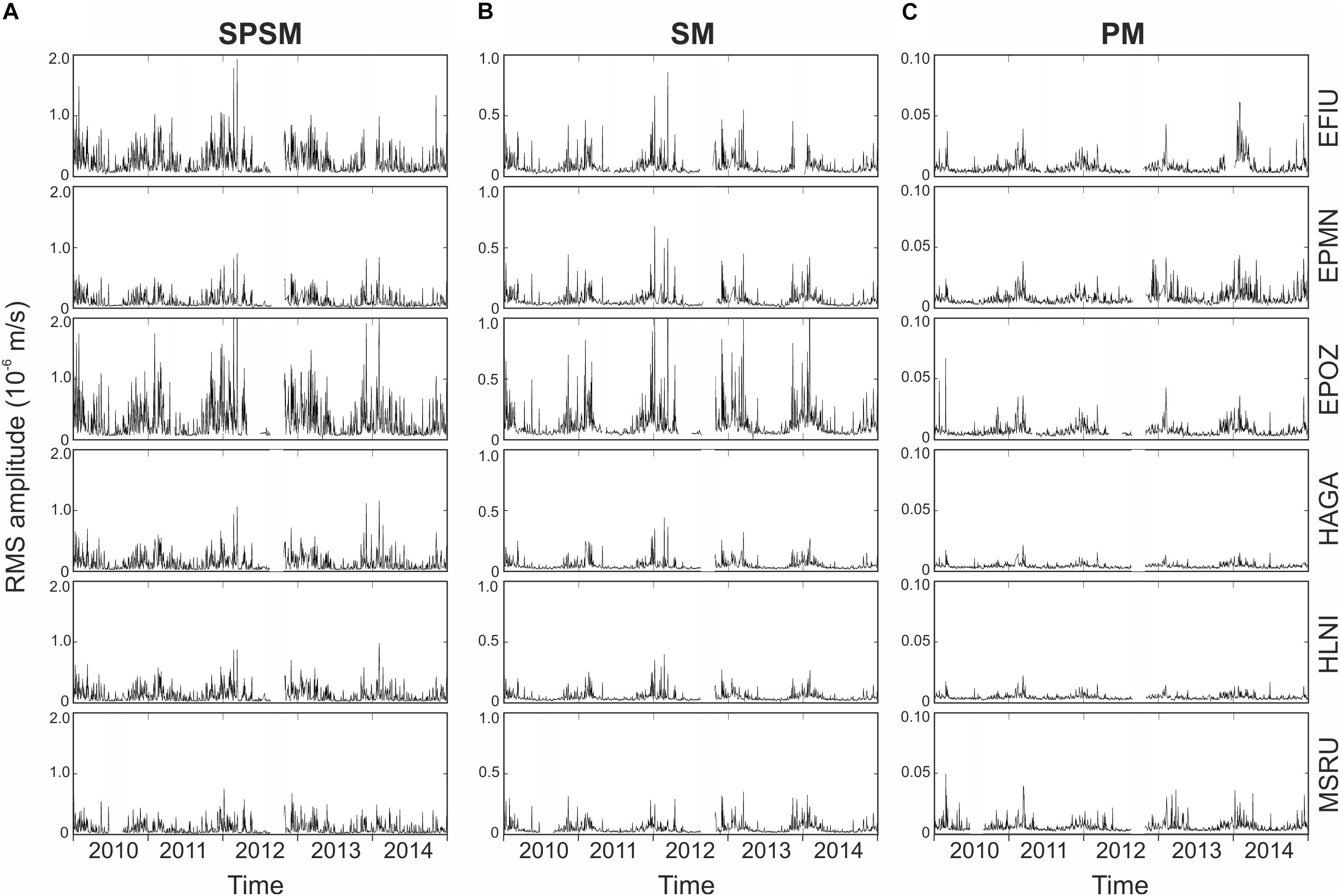
Figure 4. RMS amplitude time series of the seismic signal recorded by the vertical component of the six considered stations and filtered in the bands (A) 2.5–5.0 s (SPSM, short-period secondary microseism); (B) 5–10 s (SM, secondary microseism); and (C) 13–20 s (PM, primary microseism).

FIGURE 5

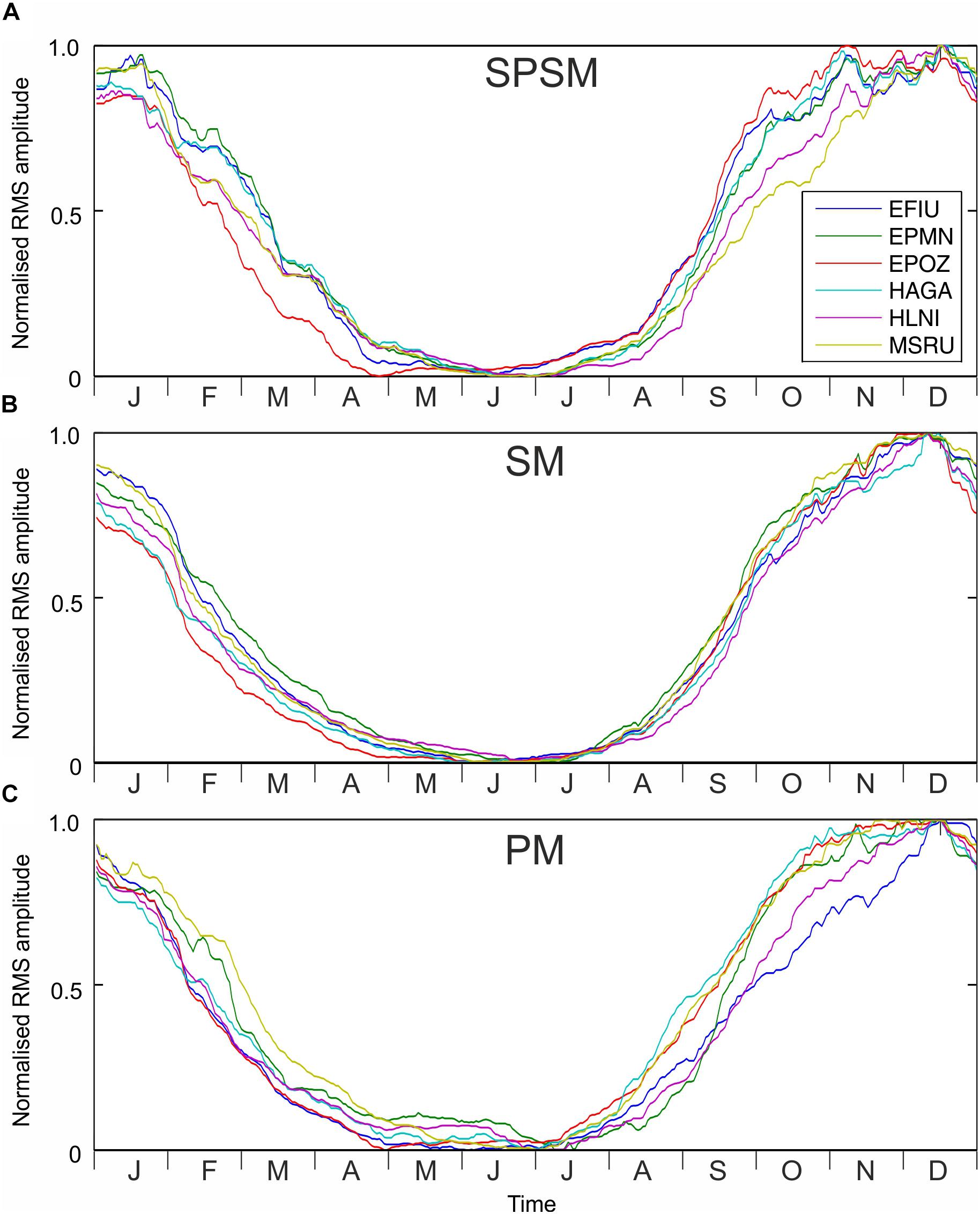
Figure 5. RMS amplitude time series smoothed by a 90-day-long moving median, split into 1-year-long windows, stacked, and normalized for all the considered seismic stations (see the legends on the bottom right corner of (A). In particular, regarding the period bands (A) 2.5–5 s (SPSM), (B) 5–10 s (SM), and (C) 13–20 s (PM). The time on the x-axis of (A–C) indicates the window onset of the 90-day-long moving median.

Array Analysis

To get an idea on the locations of the main microseism sources surrounding the Eastern Sicilian coastlines, the seven stations composing the summit ring of the Mt. Etna seismic permanent network were used as a roughly circular array (Figure 1b). The array response functions (ARFs) were computed for the PM, SM, and SPSM for a plane wave arriving with a slowness of 0 s deg^–1 (Figure 6). Such ARFs exhibit that only the SPSM case shows a fairly good resolution. This is due to the very long wavelength of PM and SM compared to the array aperture (∼5 km). Indeed, taking into account a velocity of the S-waves (V_s) in the first kilometers of the crust equal to ∼2 km/s (e.g., Hirn et al., 1991; Patanè et al., 1994), the wavelengths of PM, SM, and SPSM are ∼26, 10, and 5 km, respectively. When the wavelength is much greater than the array aperture (as in the case of PM and SM), the array behaves like a single station (e.g., Schweitzer et al., 2012).

FIGURE 6

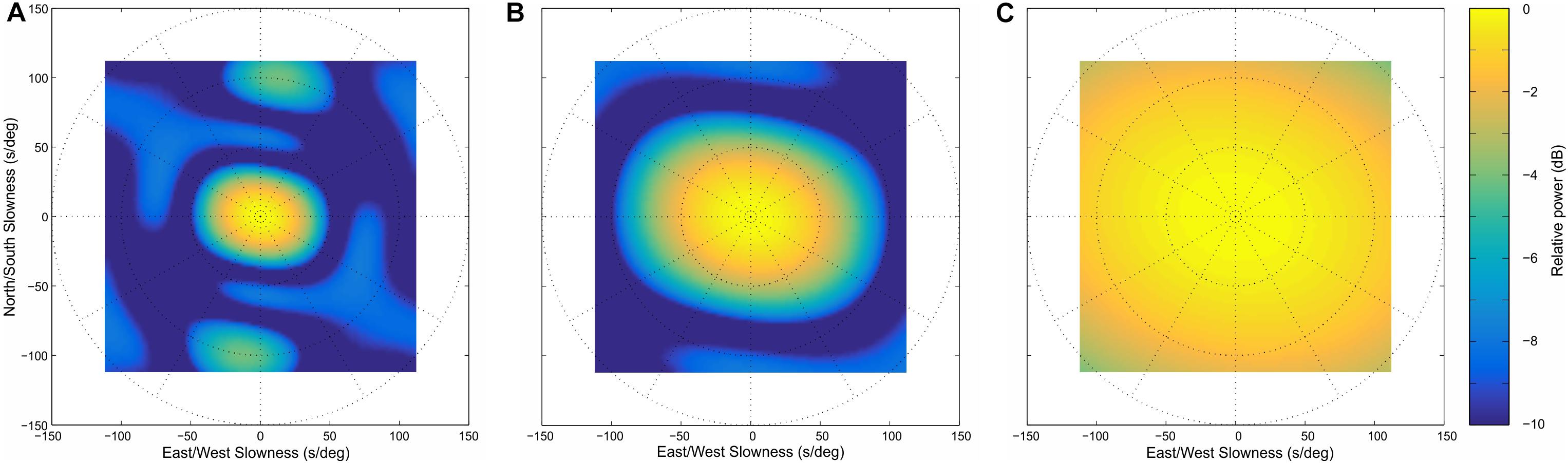
Figure 6. Array response functions of the seven stations composing the summit ring of the Mt. Etna seismic permanent network (see Figure 1b) for a unit amplitude incident wave with slowness of 0 s deg^{– 1} at periods of 2.5 s (A), 5 s (B), and 13 s (C).

The portions of the Ionian and Tyrrhenian coastlines, where the microseism sources closest to the array could supposedly be located, are characterized by a minimum distance of ∼20 and ∼45 km, respectively, from the array center. Such distances are greater than two to three times the array aperture, and hence, on the basis of the synthetic tests performed by Almendros et al. (2002), the Etna summit ring array should be able to locate the microseism sources with a planar wavefront assumption.

Then, to apply array analysis, the following processing steps were carried out on the seismic signals: demeaning and detrending, correction for the instrument response, filtering within a 0.2- to 0.40-Hz band by a second-order Butterworth filter, and subdivision in 60-s-long windows, tapered with a Tukey window. The filter is also used to exclude volcanic tremor, whose energy at Mt. Etna is mainly radiated in the band 0.5–5.0 Hz (Cannata et al., 2010). Successively, the STA/LTA technique (acronym for short time average over long time average; e.g., Trnkoczy, 2012) was applied to detect prospective amplitude transients that could be related to volcano activity (i.e., long period events and very long period events). Windows containing amplitude transients were excluded from the array analysis. Finally, the frequency–wavenumber (f–k) analysis was carried out, allowing to calculate the power distributed among different slownesses and back azimuths (e.g., Capon, 1973; Rost and Thomas, 2002).

The array analysis was performed in January 2010–February 2012 on specific time intervals characterized by one of the following two conditions: (i) intense wave activity in the Ionian Sea, as shown by the Catania buoy data and/or by the high RMS amplitude values at EPOZ station; or (ii) intense wave activity in the Tyrrhenian Sea, as suggested by the Cetraro buoy data and/or by the high amplitude RMS values at MSRU station. Examples of the results for the days 26/04/2011 and 18/12/2011, exhibiting conditions (i) and (ii), respectively, are shown in Figures 7, 8.

FIGURE 7

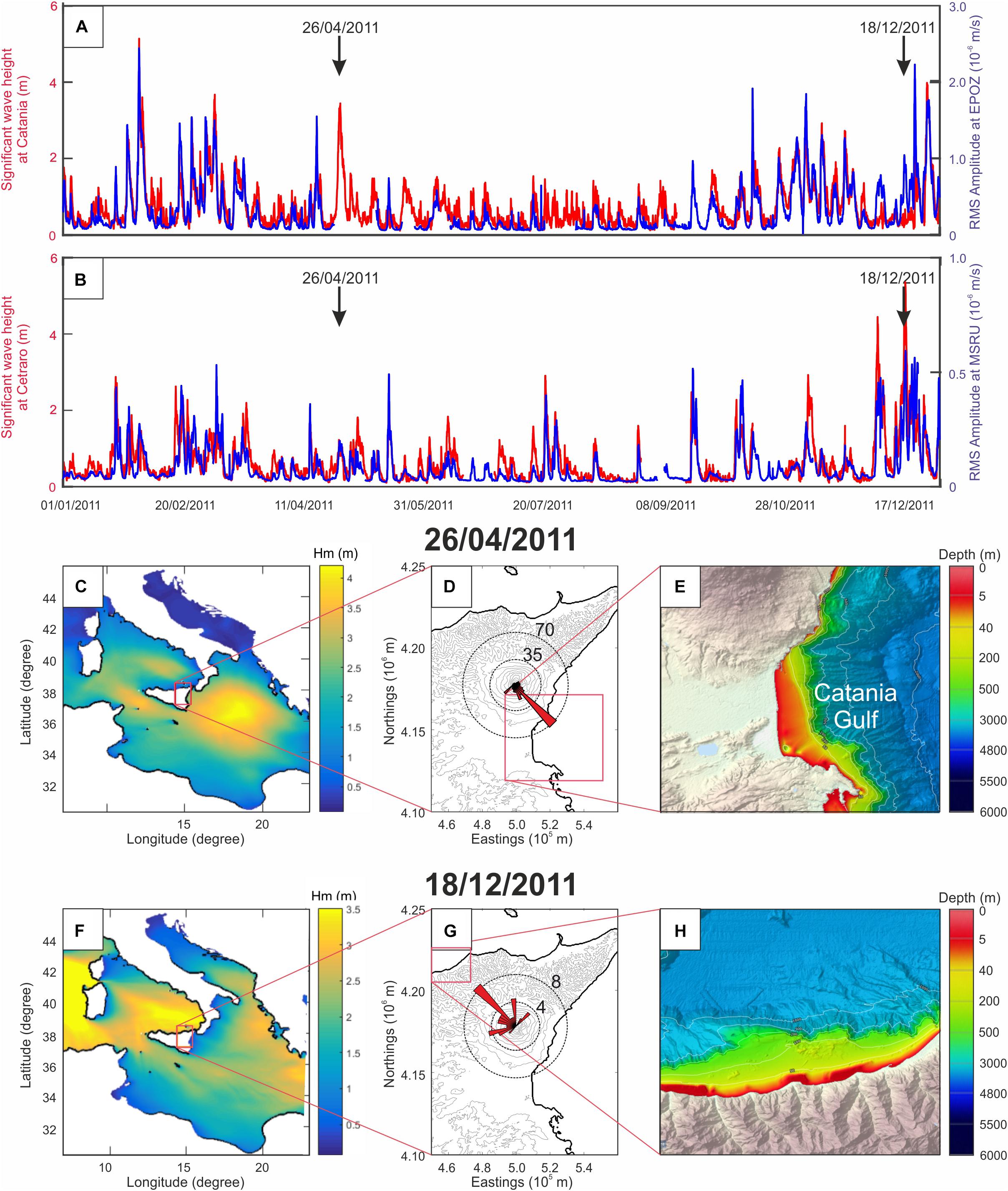
Figure 7. (A,B) Time series of significant sea wave height recorded by the Catania and Cetraro buoys (red lines) and the RMS amplitude computed in the period band 2.5–5.0 s (SPSM) by EPOZ and MSRU stations (blue lines) in 2011. (C,F) Maps of a portion of the Mediterranean Sea showing the spatial distribution of the significant wave height on 26/04/2011 at 12:00 and on 18/12/2011 at 12:00, respectively (MEDSEA_HINDCAST_WAV_006_012 product from http://marine.copernicus.eu/services-portfolio/access-to-products/). (D,G) Digital elevation models of Eastern Sicily with rose diagrams, located at the center of the seismic summit ring of Mt. Etna (see Figure 1b), showing the distribution of the back azimuth values on 26/04/2011 and 18/12/2011, computed by f–k analysis. (E,H) Maps showing the bathymetry of portions of Sicily coastlines (EMODnet Bathymetry Consortium, 2018).

FIGURE 8

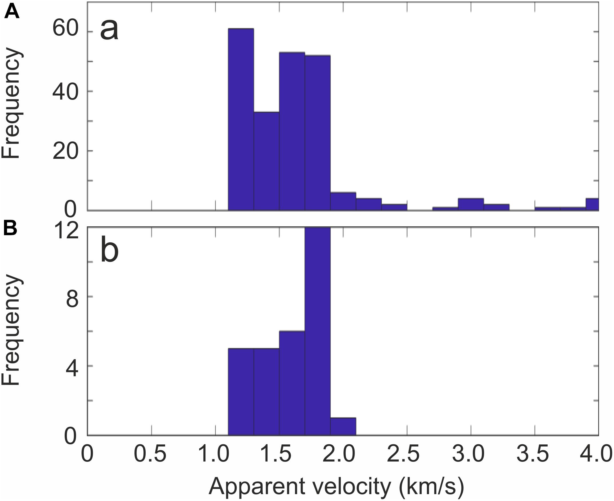
Figure 8. Histograms showing the apparent velocity estimated by f–k analysis on 26/04/2011 (a) and on 18/12/2011 (b).

To evaluate the error associated with the back azimuth estimation, the jackknife technique (Efron, 1982) was employed as follows. Firstly, the signal window was analyzed by the f–k technique by using all the seven stations composing the array. Successively, the analysis was repeated seven times, leaving one station out at a time, so providing further seven back azimuth values. An arithmetic mean of these estimates was assessed by the following equation:

$$\overline{P}=\frac{1}{n}\sum _{i=1}^n{P}_i(3)$$

where P_i is the back azimuth value computed by omitting the i-th station and n is the number of stations composing the array. Then, it is possible to estimate the i-th so-called pseudovalue as:

$$J_i=n\widehat{P}-(n-1)P_i(4)$$

where $\widehat{P}$ is the back azimuth value computed by considering all the seven array stations. The jackknife estimator of parameter P is given by:

$$J(\widehat{P})=\frac{1}{n}\sum _{i=1}^n{J}_i=n\widehat{P}-(n-1)\overline{P}(5)$$

The standard error of the jackknife estimates is given by:

$$\mathrm{\delta }{}_{J(\widehat{P})}=\sqrt{\frac{1}{n(n-1)}\sum _{i=1}^n{(J_i-J(\widehat{P}))}^2}(6)$$

Finally, median error estimations were calculated separately for the back azimuths oriented toward the Ionian Sea and the Tyrrhenian Sea [the above-mentioned conditions (i) and (ii)].

Regression Analysis by Machine Learning

Modern MLTs have been tested to build reliable predictive models able to calculate the time series of significant wave height from microseism data. The method, similar to the one proposed by Cannata et al. (2019) to spatially and temporally reconstruct the sea ice distribution around Antarctica based on the microseism amplitudes, is composed of four main steps (summarized in Figure 9): (a) data preparation; (b) training; (c) cross-validation; and (d) testing.

FIGURE 9

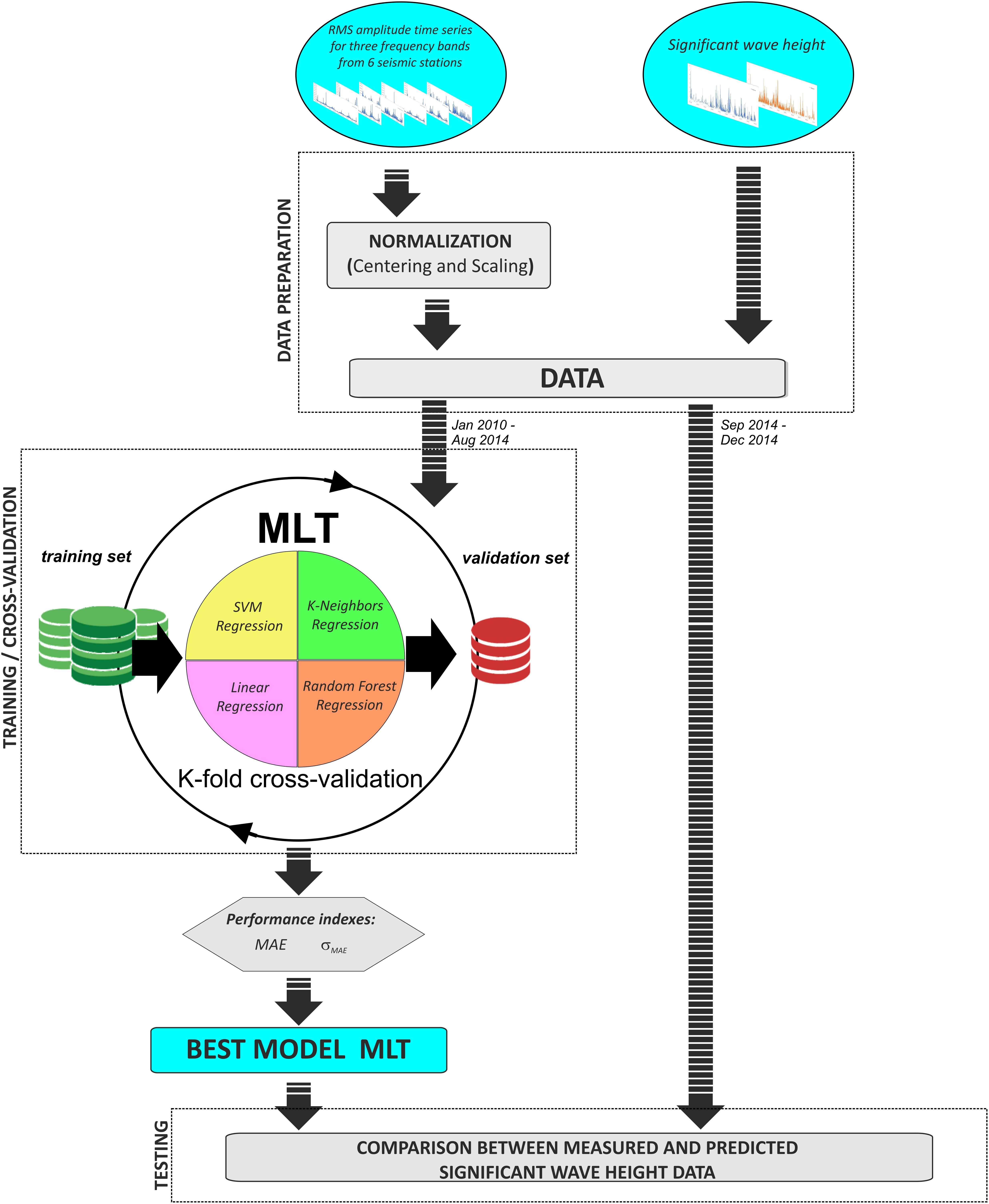
Figure 9. Scheme of the modeling analysis to obtain the time series of significant wave height in the Catania and Cetraro buoy locations by using the microseism (see text for details). MLT, machine learning technique; MAE, mean absolute error; “σ_MAE”, standard deviation computed on the mean absolute error; SVM support vector machine.

Step (a) consisted of centering and scaling the predictor variables (Kuhn and Johnson, 2013), that is, the 18 time series of the microseism hourly RMS amplitudes from January 2010 to August 2014 (six stations by three frequency bands). The remaining data (September–December 2014) is used for testing step (d). To center the microseism predictor, the average is subtracted from all the values. Successively, to scale the data, each value of the microseism predictor is divided by its standard deviation. Hence, all the time series of the microseism RMS amplitudes share a common scale.

As for step (b), we made use of the following four MLTs to build predictive models: (i) random forest (RF) regression; (ii) K-nearest neighbors (KNN) regression; (iii) linear regression; and (iv) support vector machine (SVM) regression.

As for the RF technique, it is based on decision trees often used for classification and regression (Ho, 1995). One of the main problems with decision trees is the need to increase accuracy and avoid overfitting at the same time (Ho, 1998). RF overcomes such a limitation by generating many decision trees and aggregating their results (Liaw and Wiener, 2002). Recently, RF has had many applications in geosciences, such as geochemical mapping (Kirkwood et al., 2016) and the lithological classification of underexplored areas by geophysical and remote sensing data (Kuhn et al., 2018).

K-nearest neighbors is a non-parametric technique applied for both classification and regression tasks (Altman, 1992). KNN regression simply predicts a new sample using the K-closest samples from the training set (Altman, 1992; Kuhn and Johnson, 2013). Hence, for a new input, the output is the average of the values of its K-nearest neighbors in the feature space of the training set. Such a method has been extensively used to classify remote sensing images (e.g., Li and Cheng, 2009; Noi and Kappas, 2018).

Concerning linear regressions, relationships are modeled using linear predictor functions; that is, the relationship between predictors and responses falls along a hyperplane (Kuhn and Johnson, 2013). Such linear relationships can be written as (Kuhn and Johnson, 2013):

$$y_i=b_0+b_1{x}_{i1}+b_2{x}_{i2}+\mathrm{\cdots }+b_n{x}_{in}+e_i(7)$$

where y_i is the output for the i-th sample, b₀ is the estimated intercept, b_j represents the coefficient for the j-th predictor, x_ij represents the value of the j-th predictor for the i-th sample, and e_i represents random error for the i-th sample. Similar to the two previous machine learning methods, linear regressions have been used in many fields of Earth Sciences, such as iron mineral resource potential mapping (Mansouri et al., 2018) and catchment-level base cation weathering rates (Povak et al., 2014).

Finally, SVMs are supervised learning models for both classification and regression analysis (e.g., Drucker et al., 1997; Kuhn and Johnson, 2013). As for regression, the SVM’s goal is to find a function that deviates from each training point by a value no greater than a chosen constant, and at the same time is as flat as possible (e.g., Vapnik, 2000; Kuhn and Johnson, 2013). Also, SVM has been applied in Earth Sciences, for instance to map landslide susceptibility (Reza Pourghasemi et al., 2013) and to classify remote sensing data (Jia et al., 2019).

Each of the four aforementioned techniques has its own advantages and disadvantages (e.g., Kuhn and Johnson, 2013; Yang et al., 2019). The main advantages of RF are its high accuracy and robustness to outliers and noise; also, RF parameter tuning does not have a drastic effect on performance. The disadvantages are the expensive training time and overfitting in the case of small datasets. KNN is effective and non-parametric, but it is not robust in the presence of noise and it is not easy to identify the best K value. As for linear regressions, they require short training times, and the results are easy to visualize and understand, but they are not suited to model non-linear relationships. Finally, SVMs are easy to implement and show good efficiency in training and generalization, but the tuning of parameters can be quite difficult.

For all the above-mentioned MLTs, the 18 time series of the centered and scaled seismic RMS amplitudes from January 2010 to August 2014 were used as the input, while the two time series of significant wave heights, recorded by the Catania and Cetraro buoys, were resampled by a sampling step of 1 h (the same rate as the seismic RMS amplitude time series) and considered as the output to build the regression models.

Step (c) consisted of evaluating the best MLT by carrying out the k-fold cross-validation (Kuhn and Johnson, 2013). The cross-validation implies partitioning the original input and output datasets into complementary subsets, constraining a model on one subset (called “training set”), and validating the model performance on the other subset (called “validation set”). In particular, in the performed k-fold cross-validation, the microseism amplitude and significant wave height samples are partitioned into 10 (k = 10) sets of consecutive samples. Ten models are trained by using all samples except one subset, which is used to validate the models. The parameters we used to estimate the model performance are: mean absolute error (MAE) between the observed significant wave height and the predicted one and the corresponding standard deviation (σ_MAE). The former was estimated by the following equation:

$$\text{MAE}=\frac{{\sum }_{i=1}^n\left|y_i-x_i\right|}{n}(8)$$

where x_i and y_i are the predicted and observed significant sea wave height values at the i-th time sample and n is the number of samples in x and y. The results are shown in Figures 10A,B.

FIGURE 10

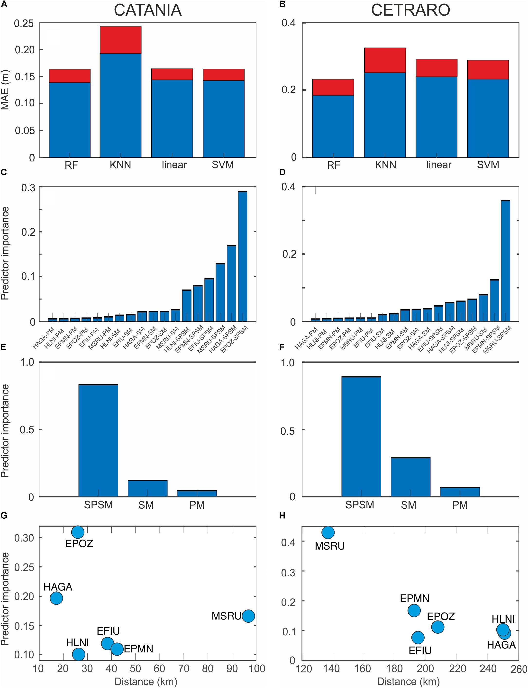
Figure 10. Results of the machine learning analysis. (A,B) Average (blue bars) and standard deviation (red bars) of the mean absolute error (MAE), estimated by k-fold cross-validation, for the Catania and Cetraro buoy data, respectively. (C,D) Index of importance for all the input taken into account to model the Catania and Cetraro buoy data, respectively. (E,F) Aggregation through a summation of the input importance allowing to rank the microseism bands for the Catania and Cetraro buoy data prediction, respectively. (G,H) Aggregation through a summation of the station importance for the Catania and Cetraro buoy data prediction plotted versus the distance from the Catania and Cetraro buoys, respectively.

The final model was trained with the whole dataset from January 2010–August 2014 and tested on the test set from September–December 2014 [testing step (d)]. The comparisons between the predicted and measured significant wave heights for the testing period are reported in Figures 11–14.

FIGURE 11

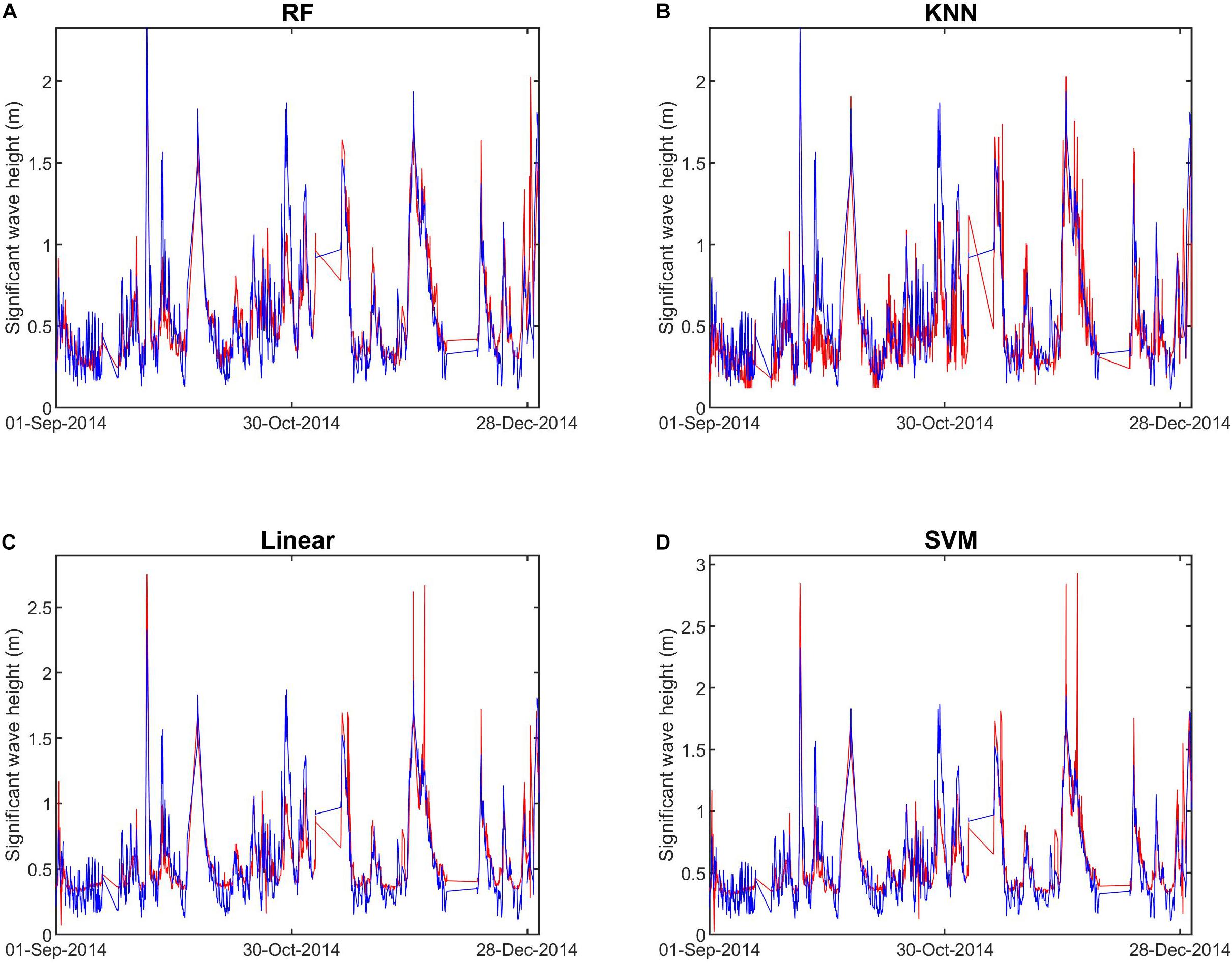
Figure 11. Measured (blue line) and predicted (red line) significant wave height time series of the Catania buoy from 1 September to 31 December 2014. The prediction was carried out by RF regression (A), KNN regression (B), linear regression (C), and SVM regression (D).

FIGURE 12

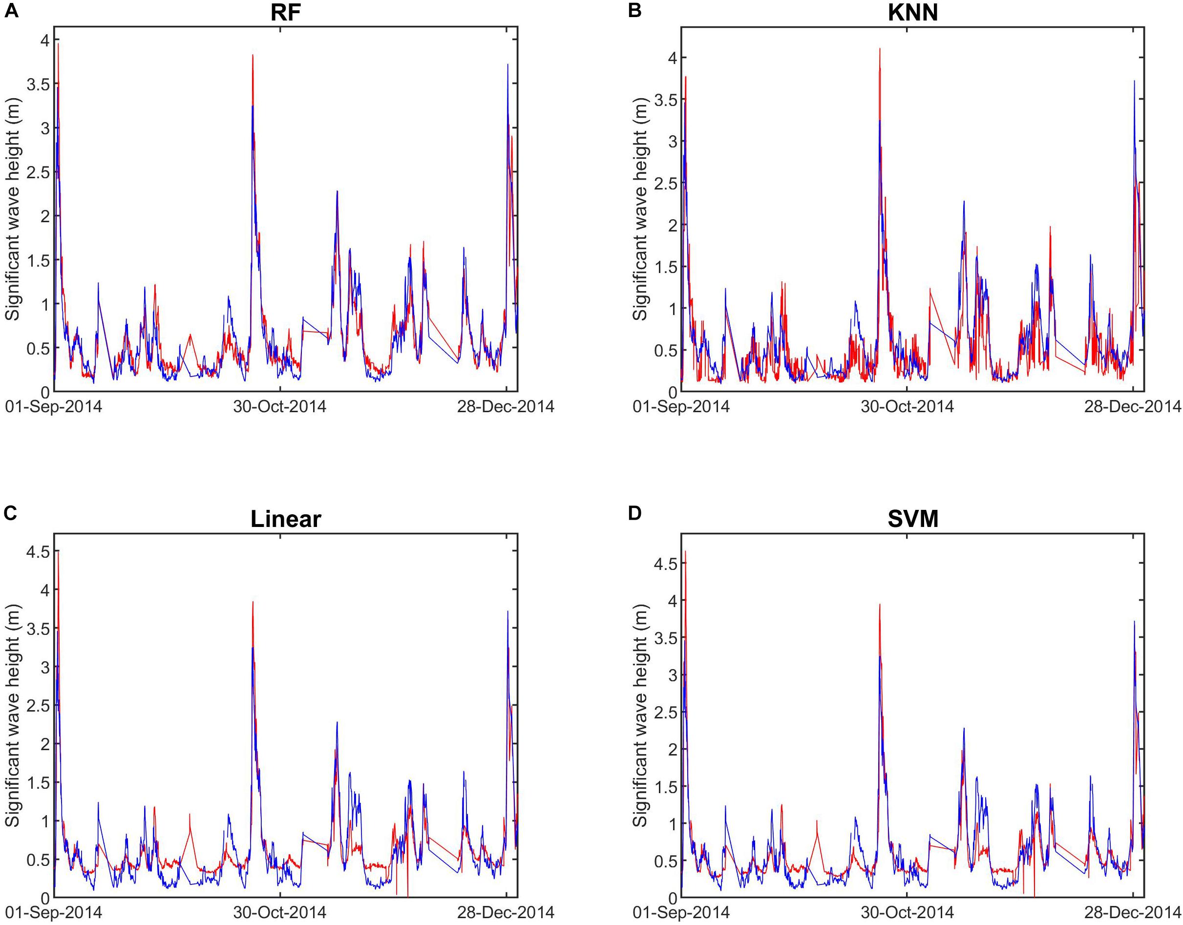
Figure 12. Measured (blue line) and predicted (red line) significant wave height time series of the Cetraro buoy from 1 September to 31 December 2014. The prediction was carried out by RF regression (A), KNN regression (B), linear regression (C), and SVM regression (D).

FIGURE 13

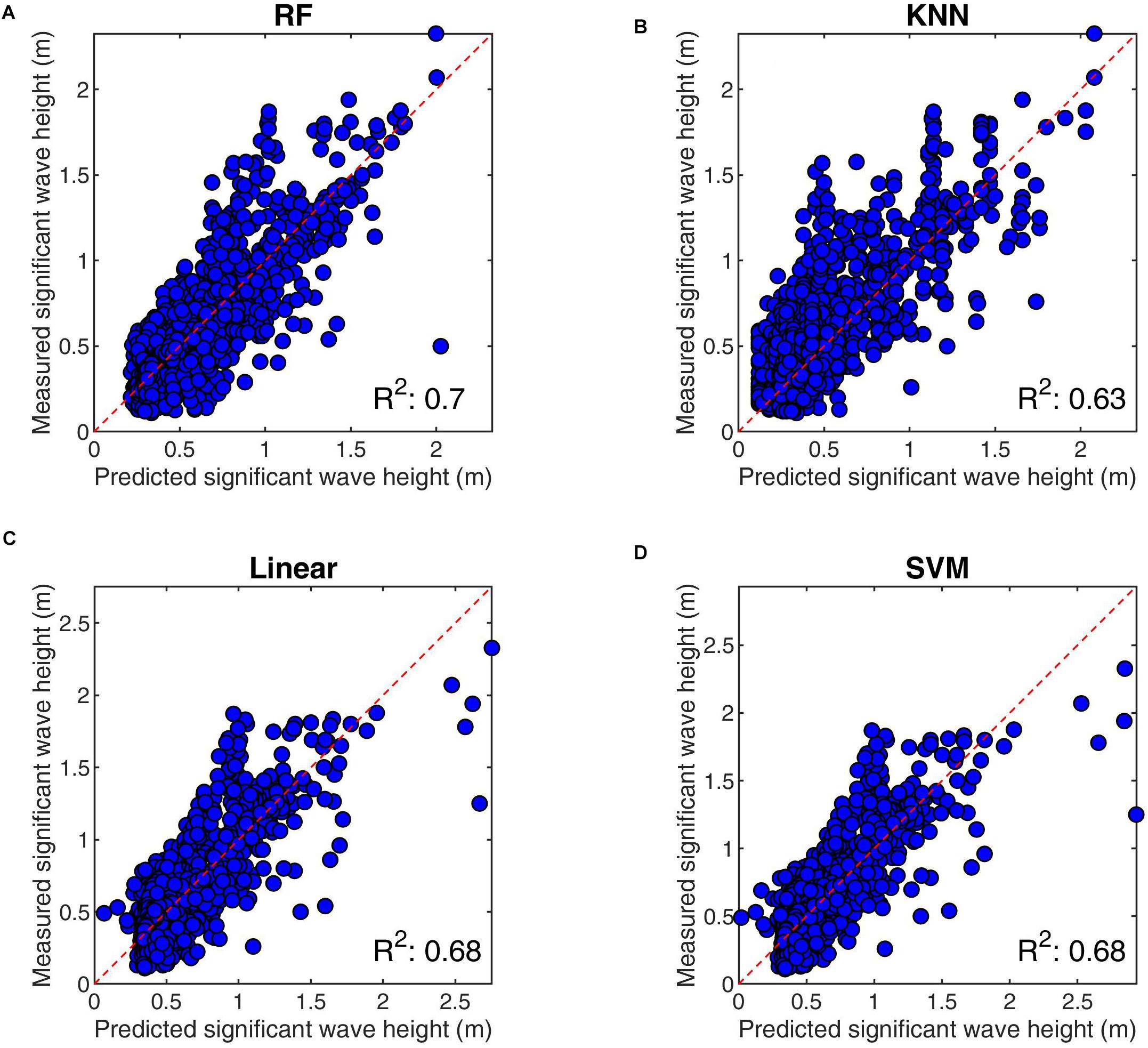
Figure 13. Scatter plots showing the measured versus the predicted significant wave heights of the Catania buoy from 1 September to 31 December 2014. The prediction was carried out by RF regression (A), KNN regression (B), linear regression (C), and SVM regression (D). The red dashed line in (A–D) is the y = x line. The value of the determination coefficient (R²) is also reported in the bottom right corner of the plots.

FIGURE 14

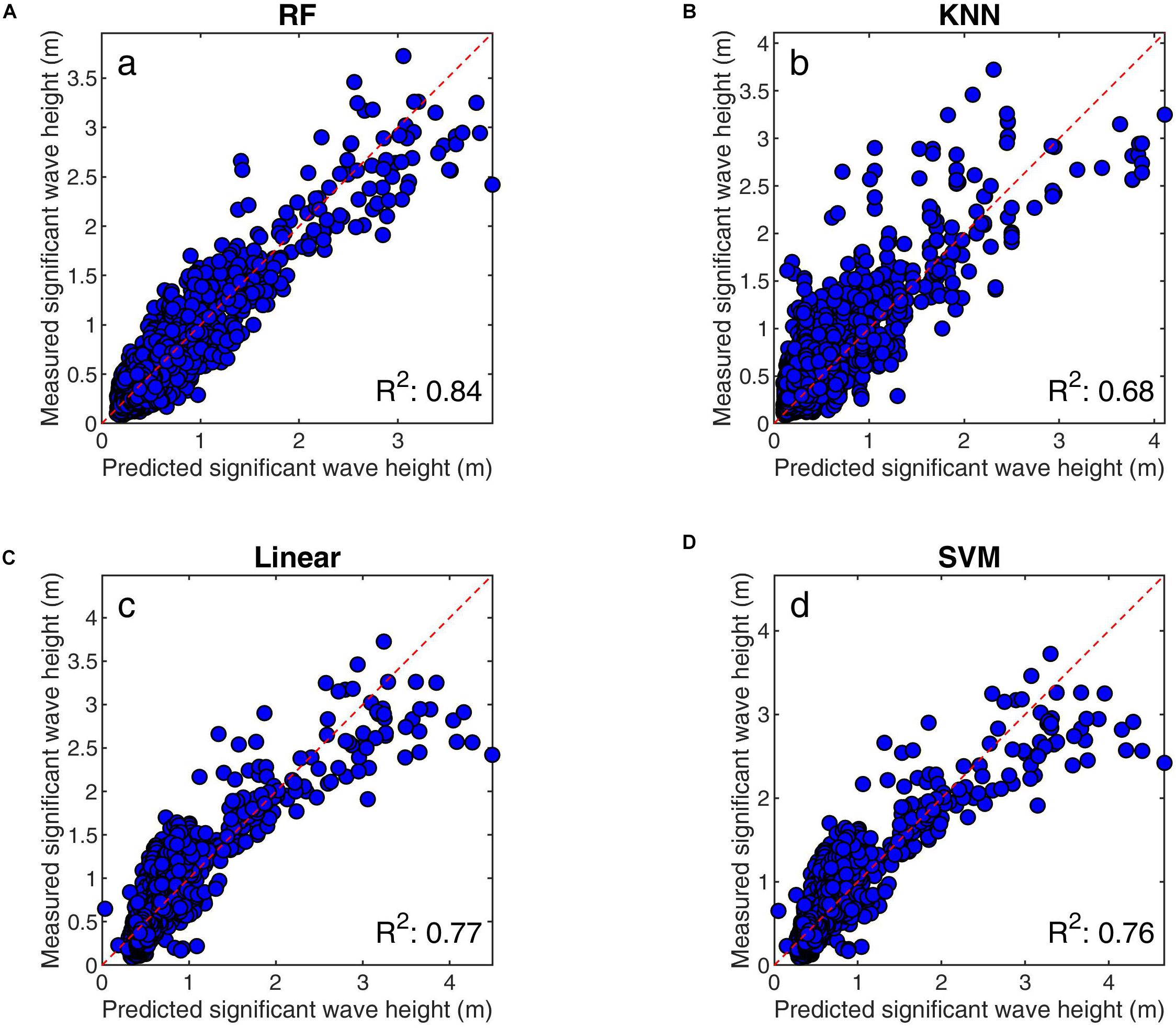
Figure 14. Scatter plots showing the measured versus the predicted significant wave heights of the Cetraro buoy from 1 September to 31 December 2014. The prediction was carried out by RF regression (A), KNN regression (B), linear regression (C), and SVM regression (D). The red dashed line in (A–D) is the y = x line. The value of the determination coefficient (R²) is also reported in the bottom right corner of the plots.

Results

Microseism recorded in Eastern Sicily shows the highest amplitude in the bands 2.5–5.0 and 5–10 s (SPSM and SM, respectively) at all the considered stations (Figures 3, 4). Moreover, evident amplitude seasonal modulation is shown in Figures 4, 5, with maxima reached during the winter (December–February) and minima during the summer (June–August).

As for the array analysis, the summit ring of Mt. Etna seismic permanent network turned out to be effective in locating the microseism sources in the SPSM band (Figure 6A). During Ionian stormy days, the back azimuth values indicate the Catania Gulf, while during Tyrrhenian stormy days the back azimuth rotates, pointing north–westward. In both cases, the SPSM sources appear to be located in areas of extended shallow water depths (Figure 7). Concerning the median error in the back azimuth estimations obtained by the jackknife technique, it was equal to 21° and 12° for back azimuths oriented toward the Tyrrhenian and Ionian Seas, respectively. As for the apparent seismic velocity estimations, the histograms in Figure 8 show values of ∼1.5–2.0 km/s.

Finally, MLTs have been able to reconstruct the time series of significant sea wave height on the basis of microseism data. The technique showing the best performance was RF regression (Figures 10A,B), allowing to get the minimum MAEs equal to 0.14 ± 0.02 m and 0.18 ± 0.05 m for the Catania (the Ionian Sea) and Cetraro (the Tyrrhenian Sea) data, respectively. It has to be underlined that the RF, linear, and SVM regressions show very similar MAE values, especially in the case of the Catania buoy. The RF approach has the advantage of easily supplying an index of predictor importance (Figures 10C,D), calculated by exploiting the random permutation of out-of-bag samples (Breiman, 2001). To get information on the importance of the different microseism bands in the prediction, aggregation through summation was performed (Figures 10E,F), showing how the SPSM band has the highest weight in reconstructing the significant wave height time series at the two buoys. In addition, aggregation through summation was performed also for the station importance and exhibited how the importance tends to decrease with increasing distance of station–buoy (Figures 10G,H).

Finally, the comparison between the measured and predicted significant wave height data during the testing period (September–December 2014; Figures 11–14) showed very similar patterns for the two time series, as also confirmed by the high values of determination coefficient equal to 0.7 and 0.84 for the Catania and Cetraro buoys, respectively, in the case of RF regressions.

Discussion and Conclusion

We investigated the microseism recorded close to the Eastern Sicily coasts and its relationship with the significant wave height recorded by two buoys installed in the Ionian and Tyrrhenian Seas. Concerning the microseism characterization, as measured in the seismic signals acquired worldwide (e.g., Aster et al., 2010), most of its energy is contained in the SPSM and SM bands (Figures 3, 4). Also, the observed seasonal amplitude modulations (Figures 4, 5) are a common feature of the microseism recorded at temperate latitudes, characterized by stormier seas during the winters (e.g., Aster et al., 2008; Stutzmann et al., 2009).

Taking into account the array analysis, performed by the seven seismic stations in Figure 1b by the f–k array technique in the SPSM band, we were able to obtain the slowness vector direction and, therefore, to get an idea on the locations of the microseism source in the SPSM band. It was observed that the SPSM sources appear to be located in areas of extended shallow water depths: the Catania Gulf and a part of the Northern Sicily coastlines (Figure 7).

The array analysis results are in agreement with Chen et al. (2011), who analyzed microseism data collected in Taiwan and showed how a stronger excitation in SPSM takes place in the narrow Taiwan Strait where the water depth is very shallow, while the excitations are relatively weak in the eastern offshore area, an open sea with water depth increasing rapidly off the coast. Although Juretzek and Hadziioannou (2017) focused on a different frequency band (PM), they also constrained the source locations of the microseism recorded in Europe in regions with extended shallow water areas, that is, Norwegian and Scottish coasts.

It has to be noted that the error associated with the microseism source locations is higher in the case of the Northern Sicily coastlines compared to the Catania Gulf. It derives from both the higher back azimuth error (21° for the Tyrrhenian Sea versus 12° for the Ionian Sea) as well as from the longer distance array–Northern Sicily coastlines (∼45 km) compared to the distance array–Catania Gulf (∼20 km).

The apparent seismic velocity estimations of 1.5–2.0 km/s in the SPSM band (Figure 8) are in agreement with the Rayleigh wave velocity calculated by using beamforming analysis, applied on the ambient seismic noise in New Zealand, by Brooks et al. (2009), as well as with the results obtained from investigating the seismic noise in the northeast of the Netherlands by Kimman et al. (2012). In addition, Rivet et al. (2015) also estimated comparable velocities (of 1.5 km/s at 1 Hz and 2.0 km/s at 0.5 Hz) by using a time–frequency analysis to measure the group velocity of Rayleigh wave on noise cross-correlation.

Finally, we propose an innovative method, based on up-to-date MLTs, able to reconstruct the time series of significant wave height by using microseism recorded in different period bands by distinct seismic stations. Such a method allows to reliably compute the significant wave height in two locations, coinciding with the two buoys in the Ionian and Tyrrhenian Seas, with fairly low error (MAE equal to ∼0.14 m for the Catania buoy and ∼0.18 m for the Cetraro buoy; Figures 10A,B). In particular, the MLT which showed the best performance was the RF regression. This can be related to several factors, such as: (i) the performance of the RF regression is not much affected by parameter selection (e.g., Li et al., 2011; Kuhn and Johnson, 2013); (ii) by making use of an ensemble of decision trees, RF regression does not overfit with respect to the source data (e.g., Li et al., 2011); and (iii) RF shows robustness to outliers and noise (Breiman, 2001). Finally, compared to linear regressions, RF regression is able to deal with non-linear relationships between the input and output. Indeed, according to Essen et al. (2003) and Craig et al. (2016), the relationship linking microseism amplitude and significant wave height is likely to be non-linear.

Focusing on the comparison between the highest measured and predicted (by RF regression) significant wave height data during the testing period, it is possible to note a slight underestimation and overestimation of the predicted values compared to the measured ones in the Catania and Cetraro cases, respectively (Figures 13A, 14A). These different behaviors could be related to the different distances between the seismic stations and the buoys.

Although buoys are considered the most used and reliable instruments for in situ measurements of sea waves (Orasi et al., 2018), the high maintenance costs, together with the recurring damages and then lack of data, make the proposed microseism-based method a valid complementary tool for the monitoring of the sea state. Furthermore, once the regression model has been determined and if the seismic data are available, such a method could allow reconstructing the time series of sea wave height during periods prior to the buoy installation, with wide applications in many fields, first of all climate studies.

The RF regression also provides an index of importance of the distinct predictor variables, which are the seismic RMS amplitude time series. The aggregated importance of the different frequency bands exhibits how the SPSM band contains most of the information for the buoy data reconstruction (Figures 10E,F). According to the literature (e.g., Bromirski et al., 2005; Chen et al., 2011; Gualtieri et al., 2015), such a microseism band, characterized by high frequencies and then by quick attenuation with distance, is mostly generated by sources located in relatively shallow water close to the shelf break, close to the seismic stations. Such sources are likely related to local nearshore non-linear wave–wave interaction (e.g., Bromirski et al., 2005). This is in agreement with the location of the considered buoys, close to the coastlines, in shallow water conditions (90 and 100 m for Catania and Cetraro, respectively; Bencivenga et al., 2012). Both PM and SM turned out to have a much smaller importance for the buoy data reconstruction. Indeed, as for PM, its dominant source regions can be located thousands of kilometers away from the seismic stations (Gualtieri et al., 2019). Concerning SM, it has been shown how it can also have pelagic sources in deep ocean (e.g., Chevrot et al., 2007; Kedar et al., 2008).

In addition, the difference in the predictors with the maximum importance for the two buoys (EPOZ-SPSM for the Catania buoy and MSRU-SPSM for the Cetraro buoy; Figures 10C,D) reflects the different locations of the seismic stations. Indeed, EPOZ is very close to the coastline of the Ionian Sea, where the Catania buoy is installed, while MSRU is placed nearby the Tyrrhenian Sea, where the Cetraro buoy is located (Figures 1, 10G,H). Hence, the closer the seismic station is to the sea, the more information concerning the sea state are contained in the recorded microseism. From a future perspective, this finding is important to build an experimental monitoring system of the sea conditions (mainly in terms of significant wave height) based on microseism recordings.

Data Availability Statement

Seismic data are provided by the Istituto Nazionale di Geofisica e Vulcanologia, Osservatorio Etneo-Sezione di Catania. Buoy data are provided by the Istituto Superiore per la Protezione e la Ricerca Ambientale (http://dati.isprambiente.it/dataset/ron-rete-ondametrica-nazionale/). Bathymetric data shown in Figures 1, 7 come from https://portal.emodnet-bathymetry.eu/. Hindcast maps of significant wave height shown in Figure 7 are provided by http://marine.copernicus.eu/services-portfolio/access-to-products/.

Author Contributions

SM and AC initiated the concepts. SM, AC, GD, and SG performed the seismic analyses. FC, SM, and AC performed the machine learning investigations. MF, GN, AO, and MP analyzed buoy data. All the authors wrote the manuscript and contributed to the interpretation of results.

Conflict of Interest

The authors declare that the research was conducted in the absence of any commercial or financial relationships that could be construed as a potential conflict of interest.

Funding

This research was partially funded by Programma Nazionale di Ricerca in Antartide, grant no. PNRA14_00011, called ICE-VOLC project (“MultiparametrIC Experiment at antarctica VOLCanoes: data from volcano and cryosphere–ocean–atmosphere dynamics,” www.icevolc-project.com).

Acknowledgments

We thank the two reviewers and the Associate Editor for their critical reading of the manuscript and constructive comments, which helped us to improve the manuscript. We are indebted to the technicians of the Istituto Nazionale di Geofisica e Vulcanologia, Osservatorio Etneo-Sezione di Catania for enabling the acquisition of seismic data. This study has been conducted using E.U. Copernicus Marine Service Information. The array f–k analysis was performed by “Seizmo – Passive Seismology Toolbox,” version 0.6.16 Otgontenger 11-Jul-2014 (http://epsc.wustl.edu/g̃geuler/codes/m/seizmo/).

References

Almendros, J., Ibáñez, J. M., Alguacil, G., and Del Pezzo, E. (2002). Array analysis using circular-wave-front geometry: an application to locate the nearby seismo-volcanic source. Geophys. J. Int. 136, 159–170. doi: 10.1046/j.1365-246x.1999.00699.x

CrossRef Full Text | Google Scholar

Altman, N. S. (1992). An introduction to kernel and nearest-neighbor nonparametric regression. Am. Stat. 46, 175–185. doi: 10.1080/00031305.1992.10475879

CrossRef Full Text | Google Scholar

Ardhuin, F., Balanche, A., Stutzmann, E., and Obrebski, M. (2012). From seismic noise to ocean wave parameters: general methods and validation. J. Geophys. Res. 117:C05002. doi: 10.1029/2011JC007449

CrossRef Full Text | Google Scholar

Ardhuin, F., Gualtieri, L., and Stutzmann, E. (2015). How ocean waves rock the Earth: two mechanisms explain microseisms with periods 3 to 300 s. Geophys. Res. Lett. 42, 765–772. doi: 10.1002/2014GL062782

CrossRef Full Text | Google Scholar

Aster, R. C., McNamara, D. E., and Bromirski, P. D. (2008). Multidecadal climate-induced variability in microseisms. Seismol. Res. Lett. 79, 194–202. doi: 10.1785/gssrl.79.2.194

CrossRef Full Text | Google Scholar

Aster, R. C., McNamara, D. E., and Bromirski, P. D. (2010). Global trends in extremal microseism intensity. Geophys. Res. Lett. 37:L14303. doi: 10.1029/2010GL043472

CrossRef Full Text | Google Scholar

Bencivenga, M., Nardone, G., Ruggiero, F., and Calore, D. (2012). The italian data buoy network (RON). Adv. Fluid Mech. 74, 321–332. doi: 10.2495/AFM120291

CrossRef Full Text | Google Scholar

Breiman, L. (2001). Random forests. Mach. Learn. 45, 5–32. doi: 10.1023/A:1010933404324

CrossRef Full Text | Google Scholar

Bromirski, P. D., and Duennebier, F. K. (2002). The near-coastal microseism spectrum: spatial and temporal wave climate relationships. J. Geophys. Res. 107:2166. doi: 10.1029/2001JB000265

CrossRef Full Text | Google Scholar

Bromirski, P. D., Duennebier, F. K., and Stephen, R. A. (2005). Mid-ocean microseisms. Geochem. Geophys. Geosyst. 6:Q04009. doi: 10.1029/2004GC000768

CrossRef Full Text | Google Scholar

Bromirski, P. D., Flick, R. E., and Graham, N. (1999). Ocean wave height determined from inland seismometer data: implications for investigating wave climate changes in the NE Pacific. J. Geophys. Res. 104, 20753–20766. doi: 10.1029/1999JC900156

CrossRef Full Text | Google Scholar

Bromirski, P. D., Stephen, R. A., and Gerstoft, P. (2013). Are deep-ocean-generated surface-wave microseisms observed on land? J. Geophys. Res. Solid Earth 118, 3610–3629. doi: 10.1002/jgrb.50268

CrossRef Full Text | Google Scholar

Brooks, L. A., Townend, J., Gerstoft, P., Bannister, S., and Carter, L. (2009). Fundamental and higher-mode Rayleigh wave characteristics of ambient seismic noise in New Zealand. Geophys. Res. Lett. 36:L23303. doi: 10.1029/2009GL040434

CrossRef Full Text | Google Scholar

Cannata, A., Cannavò, F., Moschella, S., Gresta, S., and Spina, L. (2019). Exploring the link between microseism and sea ice in Antarctica by using machine learning. Sci. Rep. 9:13050. doi: 10.1038/s41598-019-49586-z

PubMed Abstract | CrossRef Full Text | Google Scholar

Cannata, A., Di Grazia, G., Montalto, P., Ferrari, F., Nunnari, G., Patanè, D., et al. (2010). New insights into banded tremor from the 2008–2009 Mount Etna eruption. J. Geophys. Res. 115:B12318. doi: 10.1029/2009JB007120

CrossRef Full Text | Google Scholar

Capon, J. (1973). Signal processing and frequency-wavenumber spectrum analysis for a large aperture seismic array. Methods Comput. Phys. 13, 1–59. doi: 10.1016/b978-0-12-460813-9.50007-2

CrossRef Full Text | Google Scholar

Chen, Y.-N., Gung, Y., You, S.-H., Hung, S.-H., Chiao, L.-Y., Huang, T.-Y., et al. (2011). Characteristics of short period secondary microseisms (SPSM) in Taiwan: the influence of shallow ocean strait on SPSM. Geophys. Res. Lett. 38:L04305. doi: 10.1029/2010GL046290

CrossRef Full Text | Google Scholar

Chevrot, S., Sylvander, M., Benahmed, S., Ponsolles, C., Lefevre, J. M., and Paradis, D. (2007). Source locations of secondary microseisms in western Europe: evidence for both coastal and pelagic sources. J. Geophys. Res. 112:B11301. doi: 10.1029/2007JB005059

CrossRef Full Text | Google Scholar

Craig, D., Bean, C., Lokmer, I., and Möllhoff, M. (2016). Correlation of wavefield-separated ocean-generated microseisms with North Atlantic Source regions. Bull. Seism. Soc. Am. 106, 1002–1010. doi: 10.1785/0120150181

CrossRef Full Text | Google Scholar

De Caro, M., Monna, S., Frugoni, F., Beranzoli, L., and Favali, P. (2014). Seafloor seismic noise at Central Eastern Mediterranean sites. Seismol. Res. Lett. 85, 1019–1033. doi: 10.1785/0220130203

CrossRef Full Text | Google Scholar

Drucker, H., Burges, C., Kaufman, L., Smola, A., and Vapnik, V. (1997). Support vector regression machines. Adv. Neural Inform. Proc. Syst. 28, 779–784.

Google Scholar

Efron, B. (1982). The Jackknife, the Bootstrap and Other Resampling Plans. Philadelphia, PA: Soc. for Ind. and Appl. Math.

Google Scholar

EMODnet Bathymetry Consortium (2018). “EMODnet Digital Bathymetry (DTM 2018)”, in EMODnet Bathymetry Consortium. Available at: https://doi.org/10.12770/18ff0d48-b203-4a65-94a9-5fd8b0ec35f6

Google Scholar

Essen, H.-H., Krüger, F., Dahm, T., and Grevemeyer, I. (2003). On the generation of secondary microseisms observed in northern and central Europe. J. Geophys. Res. Space Phys. 2003, 1–15. doi: 10.1029/2002JB002338

CrossRef Full Text | Google Scholar

Ferretti, G., Barani, S., Scafidi, D., Capello, M., Cutroneo, L., Vagge, G., et al. (2018). Near real-time monitoring of significant sea wave height through microseism recordings: an application in the Ligurian Sea (Italy). Ocean Coast. Manag. 165, 185–194. doi: 10.1016/j.ocecoaman.2018.08.023

CrossRef Full Text | Google Scholar

Ferretti, G., Zunino, A., Scafidi, D., Barani, S., and Spallarossa, D. (2013). On microseisms recorded near the Ligurian coast (Italy) and their relationship with sea wave height. Geophys. J. Int. 194, 524–533. doi: 10.1093/gji/ggt114

CrossRef Full Text | Google Scholar

Grevemeyer, I., Herber, R., and Essen, H. (2000). Microseismological evidence for a changing wave climate in the northeast Atlantic Ocean. Nature 408, 349–352. doi: 10.1038/35042558

PubMed Abstract | CrossRef Full Text | Google Scholar

Gualtieri, L., Stutzmann, E., Capdeville, Y., Ardhuin, F., Schimmel, M., Mangeney, A., et al. (2013). Modelling secondary microseismic noise by normal mode summation. Geophys. J. Int. 193, 1732–1745. doi: 10.1093/gji/ggt090

CrossRef Full Text | Google Scholar

Gualtieri, L., Stutzmann, E., Capdeville, Y., Farra, V., Mangeney, A., and Morelli, A. (2015). On the shaping factors of the secondary microseismic wavefield. J. Geophys. Res. 120, 6241–6262. doi: 10.1002/2015jb012157

CrossRef Full Text | Google Scholar

Gualtieri, L., Stutzmann, E., Juretzek, C., Hadziioannou, C., and Ardhuin, F. (2019). Global scale analysis and modelling of primary microseisms. Geophys. J. Int. 218, 560–572. doi: 10.1093/gji/ggz161

CrossRef Full Text | Google Scholar

Hasselmann, K. A. (1963). Statistical analysis of the generation of microseisms. Rev. Geophys. Space Phys. 1, 177–210. doi: 10.1029/RG001i002p00177

CrossRef Full Text | Google Scholar

Haubrich, R. A., and McCamy, K. (1969). Microseisms: coastal and pelagic sources. Rev. Geophys. Space Phys. 7, 539–571. doi: 10.2183/pjab.93.026

PubMed Abstract | CrossRef Full Text | Google Scholar

Hirn, A., Nercessian, A., Sapin, M., Ferrucci, F., and Wittlinger, G. (1991). Seismic heterogeneity of Mt. Etna: structure and activity. Geophys. J. Int. 105, 139–153. doi: 10.1111/j.1365-246x.1991.tb03450.x

CrossRef Full Text | Google Scholar

Ho, T. (1995). “Random Decision Forests,” in Proceedings of the Third Int’l Conf. Document Analysis and Recognition, Montreal, 278–282.

Google Scholar

Ho, T. (1998). The random subspace method for constructing decision forests. IEEE Trans. Pattern Anal. Mach. Intell. 13, 340–354.

Google Scholar

Jia, K., Liu, J., Tu, Y., Li, Q., Sun, Z., Wei, X., et al. (2019). Land use and land cover classification using Chinese GF-2 multispectral data in a region of the North China Plain. Front. Earth Sci. 13, 327–335. doi: 10.1007/s11707-018-0734-8

CrossRef Full Text | Google Scholar

Jiao, P., and Alavi, A. H. (2019). Artificial intelligence in seismology: advent, performance and future trends. Geosci. Front. 19:30198. doi: 10.1016/j.gsf.2019.10.004

CrossRef Full Text | Google Scholar

Juretzek, C., and Hadziioannou, C. (2017). Linking source region and ocean wave parameters with the observed primary microseismic noise. Geophys. J. Int. 211, 1640–1654. doi: 10.1093/gji/ggx388

CrossRef Full Text | Google Scholar

Kedar, S., Longuet-Higgins, M. S., Graham, F. W. N., Clayton, R., and Jones, C. (2008). The origin of deep ocean microseisms in the North Atlantic Ocean. Proc. R. Soc. A 464, 777–793. doi: 10.1098/rspa.2007.0277

CrossRef Full Text | Google Scholar

Kimman, W. P., Campman, X., and Trampert, J. (2012). Characteristics of seismic noise: fundamental and higher mode energy observed in the Northeast of the Netherlands. Bull. Seismol. Soc. Am. 102, 1388–1399. doi: 10.1785/0120110069

CrossRef Full Text | Google Scholar

Kirkwood, C., Cave, M., Beamish, D., Grebby, S., and Ferreira, A. (2016). A machine learning approach to geochemical mapping. J. Geochem. Explorat. 167, 49–61. doi: 10.1016/j.gexplo.2016.05.003

CrossRef Full Text | Google Scholar

Kong, Q., Allen, R. M., Schreier, L., and Kwon, Y.-W. (2016). MyShake: a smartphone seismic network for earthquake early warning and beyond. Sci. Adv. 2:e1501055. doi: 10.1126/sciadv.1501055

PubMed Abstract | CrossRef Full Text | Google Scholar

Kong, Q., Trugman, D. T., Ross, Z. E., Bianco, M. J., Meade, B. J., and Gerstoft, P. (2018). Machine learning in seismology: turning data into insights. Seismol. Res. Lett. 90, 3–14. doi: 10.1785/0220180259

CrossRef Full Text | Google Scholar

Kuhn, M., and Johnson, K. (2013). Applied Predictive Modeling. New York: Springer.

Google Scholar

Kuhn, S., Cracknell, M. J., and Reading, A. M. (2018). Lithologic mapping using Random Forests applied to geophysical and remote-sensing data: a demonstration study from the Eastern Goldfields of Australia. Geophysics 82, 183–193. doi: 10.1190/geo2017-0590.1

CrossRef Full Text | Google Scholar

Lepore, S., and Grad, M. (2018). Analysis of the primary and secondary microseisms in the wavefield of the ambient noise recorded in northern Poland. Acta Geophys. 66, 915–929. doi: 10.1007/s11600-018-0194-2

CrossRef Full Text | Google Scholar

Li, J., Heap, A. D., Potter, A., and Daniell, J. J. (2011). Application of machine learning methods to spatial interpolation of environmental variables. Environ. Model. Softw. 26, 1647–1659. doi: 10.1016/j.envsoft.2011.07.004

CrossRef Full Text | Google Scholar

Li, Y., and Cheng, B. (2009). “An improved K-Nearest neighbor algorithm and its application to high resolution remote sensing image classification,” in Proceedings of the IEEE Geoinformatics Conference, Fairfax, VA, 1–4.

Google Scholar

Liaw, A., and Wiener, M. (2002). Classification and regression by random Forest. R News 2, 18–22.

Google Scholar

Longuet-Higgins, M. S. (1950). A theory of the origin of microseisms. Philos. Trans. R. Soc. Lond. Ser. A 243, 1–35. doi: 10.1098/rsta.1950.0012

CrossRef Full Text | Google Scholar

Mansouri, E., Feizi, F., Rad, A. J., and Arian, M. (2018). Remote-sensing data processing with the multivariate regression analysis method for iron mineral resource potential mapping: a case study in the Sarvian area, central Iran. Solid Earth 9:373. doi: 10.5194/se-9-373-2018

CrossRef Full Text | Google Scholar

Noi, P. T., and Kappas, M. (2018). Comparison of random forest, k-nearest neighbor, and support vector machine classifiers for land cover classification using sentinel-2 imagery. Sensors 18:18. doi: 10.3390/s18010018

PubMed Abstract | CrossRef Full Text | Google Scholar

Oliver, J., and Page, R. (1963). Concurrent storms of long and ultralong period microseisms. Bull. Seismol. Soc. Am. 53, 15–26.

Google Scholar

Orasi, A., Picone, M., Drago, A., Capodici, F., Gauci, A., Nardone, G., et al. (2018). HF radar for wind waves measurements in the Malta-Sicily Channel. Measurement 128, 446–454. doi: 10.1016/j.measurement.2018.06.060

CrossRef Full Text | Google Scholar

Patanè, D., Privitera, E., Ferrucci, F., and Gresta, S. (1994). Seismic activity leading to the 1991-1993 eruption of Mt. Etna and its tectonic implications. Acta Vulcanol. 4, 47–55.

Google Scholar

Povak, N. A., Hessburg, P. F., McDonnell, T. C., Reynolds, K. M., Sullivan, T. J., Salter, R. B., et al. (2014). Machine learning and linear regression models to predict catchment-level base cation weathering rates across the southern Appalachian Mountain region, USA. Water Resour. Res. 50, 2798–2814. doi: 10.1002/2013wr014203

CrossRef Full Text | Google Scholar

Pratt, M. J., Wiens, D. A., Winberry, J. P., Anandakrishnan, S., and Euler, G. G. (2017). Implications of Sea ice on Southern Ocean microseisms detected by a seismic array in West Antarctica. Geophys. J. Int. 209, 492–507. doi: 10.1093/gji/ggx007

CrossRef Full Text | Google Scholar

Reza Pourghasemi, H., Jirandeh, A. G., Pradhan, B., Xu, C., and Gokceoglu, C. (2013). Landslide susceptibility mapping using support vector machine and GIS at the Golestan Province. Iran. J. Earth Syst. Sci. 122, 349–369. doi: 10.1007/s12040-013-0282-2

CrossRef Full Text | Google Scholar

Rivet, D., Campillo, M., Sanchez-Sesma, F., Shapiro, N. M., and Singh, S. K. (2015). Identification of surface wave higher modes using a methodology based on seismic noise and coda waves. Geophys. J. Int. 203, 856–868. doi: 10.1093/gji/ggv339

CrossRef Full Text | Google Scholar

Rost, S., and Thomas, C. (2002). Array seismology: methods and applications. Rev. Geophys. 40:1008. doi: 10.1029/2000RG000100

CrossRef Full Text | Google Scholar

Schweitzer, J., Fyen, J., Mykkeltveit, S., Gibbons, S. J., Pirli, M., Kühn, D., et al. (2012). “Seismic arrays,” in IASPEI New Manual of Seismological Observatory Practice 2 (NMSOP-2), ed. P. Bormann (Potsdam: IASPEI). doi: 10.2312/GFZ.NMSOP-2_ch9

CrossRef Full Text | Google Scholar

Steele, K. E., and Mettlach, T. (1993). “NDBC wave data – current and planned,” in Measurement and Analysis - Proceedings of the Second International Symposium (Reston: ASCE), 198–207.

Google Scholar

Stutzmann, E., Schimmel, M., Patau, G., and Maggi, A. (2009). Global climate imprint on seismic noise. Geochem. Geophys. Geosyst. 10:Q11004. doi: 10.1029/2009GC002619

CrossRef Full Text | Google Scholar

Tanimoto, T., Heki, K., and Artru-Lambin, J. (2015). “Interaction of Solid Earth, Atmosphere, and Ionosphere,” in Treatise in Geophysics, 2nd Edn, ed. G. Schubert (Amsterdam: Elsevier), 421–444. doi: 10.1016/b978-044452748-6.00075-4

CrossRef Full Text | Google Scholar

Trnkoczy, A. (2012). “Understanding and parameter setting of STA/LTA trigger algorithm,” in IASPEI New Manual of Seismological Observatory Practice 2 (NMSOP-2), ed. P. Bormann (Potsdam: IASPEI), 1–20. doi: 10.2312/GFZ.NMSOP-2_IS_8.1

CrossRef Full Text | Google Scholar

Tsai, V. C., and McNamara, D. E. (2011). Quantifying the influence of sea ice on ocean microseism using observations from the Bering Sea, Alaska. Geophys. Res. Lett. 38:L22502. doi: 10.1029/2011GL049791

CrossRef Full Text | Google Scholar

Vapnik, V. N. (2000). The Nature of Statistical Learning Theory. New York: Springer.

Google Scholar

Welch, P. D. (1967). The use of Fast Fourier Transform for the estimation of power spectra: a method based on time averaging over short, modified periodograms. IEEE Trans. Audio Electroacoust. 15, 70–73. doi: 10.1109/TAU.1967.1161901

CrossRef Full Text | Google Scholar

Wiszniowski, J., Plesiewicz, B. M., and Trojanowski, J. (2014). Application of real time recurrent neural network for detection of small natural earthquakes in Poland. Acta Geophys. 62, 469–485. doi: 10.2478/s11600-013-0140-2

CrossRef Full Text | Google Scholar

Yang, X. S., Sherratt, S., Dey, N., and Joshi, A. (2019). Fourth International Congress on Information and Communication Technology: ICICT 2019. London: Springer Nature.

Google Scholar