 Mareen Lösing
 Jörg Ebbing
 Wolfgang Szwillus
- Institute of Geosciences, Kiel University, Kiel, Germany
Geothermal heat flux under the Antarctic ice is one of the least known parameters. Different methods (based on e.g., magnetic or seismic data) have been applied in recent years to quantify the thermal structure and the geothermal heat flux, resulting in vastly different estimates. In this study, we use a Bayesian Monte-Carlo-Markov-Chain approach to explore the consistency of such models and to which degree lateral variations of the thermal parameters are required. Hereby, we evaluate the input from different lithospheric models and how they influence surface heat flux. We demonstrate that both Curie isotherm and heat production are dominating parameters for the thermal calculation and that use of incorrect models or sparsely available data lead to unreliable results. As an alternative approach, geological information should be coupled with geophysical data analysis, as we demonstrate for the Antarctic Peninsula.
1. Introduction
As the climate changes, the Antarctic ice sheet represents a large potential source of sea level rise. However, one key parameter controlling ice sheet dynamics (e.g., Bell, 2008) remains poorly constrained: geothermal heat flux (GHF), the contribution of heat at the base of the ice sheets (Larour et al., 2012; Llubes et al., 2013). Despite some recent drilling initiatives (Risk and Hochstein, 1974; Decker and Bucher, 1982; Morin et al., 2010; Schroeder et al., 2011; Fisher et al., 2015), the remoteness and vastness of the continent limits the possibility to achieve a good, homogeneous coverage of the entire continent. Only very few GHF measurements have been taken in boreholes into subglacial lake sediments (e.g., Fisher et al., 2015) and seafloor sedimentary strata (e.g., Schroeder et al., 2011) or derived from basal temperature gradients in deep ice boreholes (e.g., Engelhardt, 2004). Further, the thick blanketing ice sheet, which covers >99% of the continent makes accessing and measuring GHF extremely challenging. Poorly-constrained thermal effects within the ice sheet itself, like ice flow, coupled with the fluctuations of surface temperatures recorded in the ice column, implies that GHF is hard to de-convolve from these other signals (Cuffey and Paterson, 2010).
However, some of the recent drilling initiatives indicate a GHF of more than 115 mW/m2, far exceeding the GHF normally measured over the continental crust (Risk and Hochstein, 1974; Morin et al., 2010; Fisher et al., 2015). Such a high GHF, especially if valid on a regional scale, indicates a remarkably hot subsurface and would clearly have an effect on ice sheet dynamics. Furthermore, this would also influence glacial-isostatic adjustment (GIA), since a hot upper mantle is less viscous. However, there are concerns that the individual high heat flux measurements reflect locally anomalous conditions and are thus not representative for a wider area (Pollack et al., 1993).
Direct measurements of heat flux can be complemented for example by exploiting the indirect sensitivity of the magnetic field, seismic wave propagation and the gravity field to the thermal structure or as by-product from ice sheet temperature modeling.
As already stated, a variety of geothermal heat flux models has been published for Antarctica over the last years (see summary in Van Liefferinge, 2018). Estimates have been done using for example satellite and airborne magnetic data (e.g., Fox Maule et al., 2005; Martos et al., 2017, Figures 1A,C). The magnetic field is affected by the temperature structure, since rocks lose their magnetic properties at the Curie temperature. This is often associated with the 580 degree isotherm, which is the Curie temperature of magnetite (e.g., Lanza and Meloni, 2006), apparently the most abundant ferromagnetic mineral in the crust. Magnetic data do not directly provide the isotherm, but are used by spectral approaches or magnetic dipole methods to define either the deepest magnetic sources (Ravat et al., 2007) or the thickness of the magnetic crust (Fox Maule et al., 2005). These are then interpreted to correlate to the Curie isotherm (e.g., Spector and Grant, 1970; Purucker et al., 1998) and by assuming some thermal parameters for the crust, the geothermal heat flux is calculated for a steady state model.
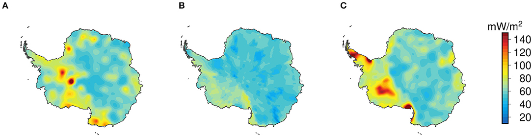
Figure 1. Geothermal heat flux models based on different geophysical methods. (A) Satellite magnetic analysis (Fox Maule et al., 2005), (B) Seismic analysis (An et al., 2015), and (C) Airborne and satellite magnetic analysis (Martos et al., 2017).
Alternatively, the propagation velocities of long-period (≥100s) surface waves are strongly sensitive to lithospheric temperature, since the shear wave velocity of mantle rocks depends strongly on temperature (e.g., Afonso et al., 2013). An et al. (2015) have used surface waves to determine the lithosphere-asthenosphere boundary (LAB) and the Curie isotherm for Antarctica. The difference between these models is significant (Figure 1) and demonstrates the need to consolidate the different methods in an integrated framework.
All these earlier studies apply specific boundary conditions, e.g., laterally constant heat production and thermal conductivity (Table 1), which are rather simplifying assumptions. While Fox Maule et al. (2005) and Martos et al. (2017) used exponentially decreasing heat production in the crust and a constant value for the crustal thermal conductivity, An et al. (2015) differentiated between upper, middle, and lower crust and upper mantle with overall lower values.
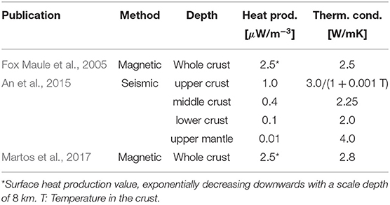
Table 1. Boundary conditions used in previous publications for surface heat flux calculations.
To reconcile the different models and/or to predict their uncertainties, Bayesian analysis can be applied that produces a variety of different combinations of the thermal parameters. We can then efficiently find an optimal model that reproduces the prior information and the input data, which in our case are lithospheric boundary depths from several different models. Furthermore, we use geological and heat production data of the Antarctic Peninsula (Burton-Johnson et al., 2017) as constraints to limit the number of variables to invert.
2. Materials and Methods
2.1. Thermal Modeling
We assume that heat flux is purely vertical (a common assumption, e.g., Afonso et al., 2013) and that the lithospheric columns are in thermal equilibrium. Then, the temperature equation becomes:
where T is the temperature, z the depth and k1 and h(z) are the heat conductivity and productivity in the crust.
We also assume that no heat is produced inside the lithospheric mantle. Thus, the temperature increases linearly with depth. The temperature gradient inside the lithospheric mantle is determined by the temperature and heat flux at the Moho boundary, since crust and mantle are assumed to be in thermal equilibrium. This leads to the following expression for the temperature structure inside the lithospheric mantle:
Here M is the Moho boundary depth, qD is the heat flux at the Moho boundary and k2 is the heat conductivity of the mantle.
In order to obtain an expression for the temperature and heat flux as a function of depth, we first define the following two quantities:
and
Integrating over the temperature equation once from z′ = 0 to z leads to an expression for the heat flux at a specific depth:
That is, the heat flux at one specific depth is always equal to the surface heat flux q0 minus the total heat production above that depth H(z).
Another integration step leads to the temperature expression:
Specifically, at the Moho boundary we find:
and likewise for the temperature:
2.1.1. Constant Heat Production
If the heat production is simply constant with depth throughout the crust, we have:
where A is the total crustal heat production. Specifically at the Moho (z = M):
The temperature distribution becomes:
2.1.2. Exponentially Decreasing Heat Production
Let us consider the case of exponentially decaying heat production. Then
where H0 is the heat production rate at the surface and hr is the scale depth at which H0 decreased to 1/e of its surface value. By integrating this, it follows:
For large z, H(z) approaches H0hr.
The second integral is:
Thus, the heat flux at the Moho becomes:
The temperature at the Moho is:
2.2. Inversion Approach
If temperature values Ti at specific depths zi are known (in our case at the surface, the Curie depth and the LAB) and we know the Moho depth M, what do we have to assume to determine geothermal heat flux? In the case of constant heat production, there are four unknown parameters: qD, A, k1, and k2, and in the case of exponentially decreasing heat production hr enters as an additional variable. Since we only have three known values, there will necessarily be trade-offs between the parameters. Alternatively, at least one parameter needs to be fixed. Furthermore, the different observations might simply be irreconcilable, i.e., no combination of parameters can explain all observations.
For these reasons, we want to explore the whole set of possible model parameters applying a Monte-Carlo-Markov-Chain (MCMC) approach.
The problem set-up is the following. For a single column, we place the thermal parameters in a vector θ. E.g., θ = (qD, A, k1, k2). The vector-valued forward operator F(θ) predicts the temperature at all isotherm depths z = (z1, z2, …) and the temperatures at the isotherms are gathered in the vector T = (T1, T2, …). The goal is then to obtain a set of θ, with F(θ) ≈ T.
In order to use the MCMC methodology, a statistical description must be used. Each θ is assigned a likelihood based on how well it fits the temperatures and how well it agrees with prior knowledge. We use an independent Gaussian misfit distribution for temperature:
where σT describes how well the temperatures should be fitted. Note that instead of keeping the depths zi fixed, we could also have used variable depths and fixed temperatures. However, this would require re-arranging the temperature equation. This is not per se challenging, but this needs to be repeated for any new heat production function. In addition, the temperature σT basically corresponds to a depth uncertainty of . For the prior we simply use independent uniform distributions with a wide range.
Using Bayes theorem, we find the following expression for the probability of a model θ:
Since the value of σT has a strong impact on the behavior of the inversion, we apply a hierarchical approach (Bodin et al., 2012) to co-invert for σT. Then, the probability is modified:
where we assume that σT is between 0 and 10 K.
In order to generate samples of θ and σT we use the Metropolis-Hastings algorithm (see Figure 2): At each iteration of the algorithm, a new value for either θ or σT is proposed. A random perturbation is added to either one randomly chosen element of θ or σT. The perturbation is drawn from a zero mean normal distribution. The probability of the new proposed model is evaluated. If it is higher than the current model's probability, the change is accepted, and the proposed model becomes the new model. If the new probability is lower than the previous probability, the new model is accepted with a probability pnew/pold. Then, the iteration proceeds with a new proposed value. The sequence of θ and σT values is called a Markov chain and samples the distribution p(θ|σT|T). However, the chain requires a certain number of burn-in iterations until its elements are representative for the distribution. For this reason, we remove the first 50, 000 out of at least 100, 000 iterations and determine the arithmetic mean of the remaining iterations as the resulting parameter. We show that the number of iterations can have an influence on the result (Figure S1) and thus, in the following we calculated the inversion with 1, 000, 000 iterations to limit the influence of random fluctuations.
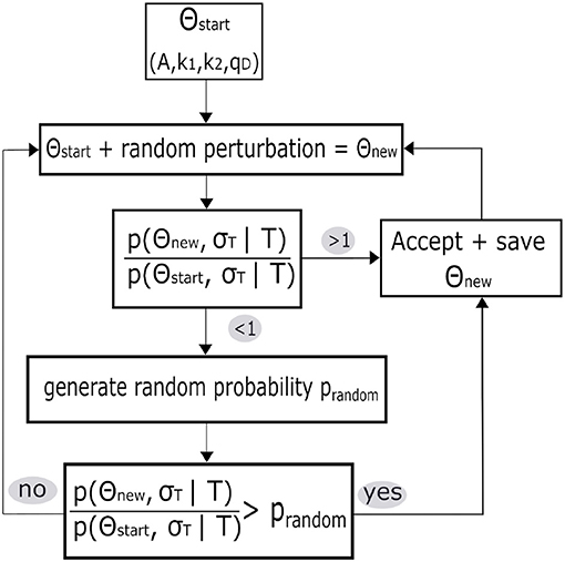
Figure 2. A simplified flow chart for the first iteration of the Metropolis–Hastings algorithm, as described in the text, for the example of a changed parameter vector.
The samples from the Markov chain can be used to derive further summary statistics like median and standard deviation. In addition the correlation between parameters can be investigated to determine which parameters are strongly interdependent and thus hard to resolve.
The applied prior range of the thermal parameters, according to the typical physical properties of crustal and mantle rocks (e.g., Turcotte and Schubert, 2014; Goodge, 2018), their start values and allowed iteration step size are given in Table 2. For the temperatures we assume values of 0°C at the surface, 580°C at the Curie depth and 1315°C at the LAB, similar to previous studies (Martos et al., 2017; An et al., 2015).
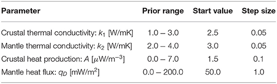
Table 2. Prior information of the thermal parameters for the inversion: allowed range, start value, and step size for each iteration.
2.3. Synthetic Test
To test the inversion, we use three synthetic columns representing very hot West Antarctica (Curie depth = 10 km, Moho depth = 25 km and LAB depth = 100 km), a slightly less hot West Antarctica (Curie depth = 20 km, Moho depth = 25 km and LAB depth = 100 km) and relatively cold East Antarctica (Curie depth = 30 km, Moho depth = 40 km and LAB depth = 220 km). The synthetic examples are used to explore which combination of thermal parameters is in agreement with the input data. Therefore, first equation 6 is solved for the crustal thermal conductivity with the given Curie depth, heat flux from 60 to 180 mW/m2 in steps of 20 mW/m2 and heat production values ranging from 0.1 to 7.0 μW/m3 (e.g., Burton-Johnson et al., 2017; Goodge, 2018). Equation (7) is then used to calculate the mantle heat flux and finally, the mantle thermal conductivity is calculated with Equation (2) and the previously determined parameters. We then limit the results only to realistic thermal conductivities (see Table 2) and get a variety of parameter combinations that are possible for the given range of GHFs and heat production rates within the synthetic columns with fixed temperatures.
A shallow Curie depth of only 10 km depth, as found by Martos et al. (2017) in West Antarctica restricts the parameter space (assuming a LAB of 100 km) to high heat production rates and a small range of possible mantle heat fluxes (Figure 3A). Only high surface heat fluxes between about 160 to 180 mW/m2 are possible in these conditions.
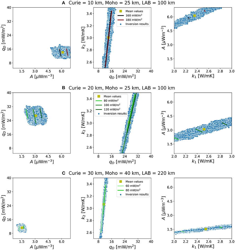
Figure 3. Correlations of possible values for mantle heat flux qD, heat production A, crustal and mantle thermal conductivity, k1 and k2, from synthetic test columns (solid lines indicating the different solutions for fixed discrete GHF values that range from 60 to 180 mW/m2 in steps of 20 mW/m2) and inversion results (blue dots). Curie isotherm, Moho and LAB depths are set for representative regions in (A) West Antarctica with a 10 km Curie depth, (B) West Antarctica with a 20 km Curie depth and (C) East Antarctica. We only plot and calculate the mean values of the final 950, 000 iterations (yellow rectangles).
Figure 3B shows that for a slightly deeper Curie depth in West Antarctica, only specifying the lithospheric structure is compatible with a wider range of GHFs (80–20 mW/m2) depending on the chosen thermal parameters. This is because the two isotherms at these depths are inherently incapable of constraining all thermal parameters. The range of possible solutions widens or thins depending on the distance between Curie and LAB depth.
For the East Antarctic case (Figure 3C), the resulting GHF is more limited, because the deep LAB limits mantle heat flux again between 9 and 14 mW/m2. Therefore, the total heat production for this synthetic column cannot exceed 2.0μW/m3. In this example, otherwise heat would be flowing from the crust into the mantle. Please note that the heat production represents an average for the crust, but that real heat productions might exceed this range on a local scale (see Goodge, 2018 and Discussion). It follows that the GHF only takes on values between 60 and 80 mW/m2. For all the cases, west or east, the possible parameter combination is most confined for the heat production—crustal thermal conductivity relation indicating that a good knowledge of one of the parameters would help to constrain the inversion considerably.
The inversion results are in the same parameter range as the synthetic input results. We calculate the mean values from these parameters which lead to calculated mean GHFs of 169.06 and 103.99 mW/m2 for West and 68.29 mW/m2 for East Antarctica. The wide parameter ranges for the western examples (besides regions with Curie depths shallower than 10 km) indicate that non-uniqueness is more problematic here and that the inversion has more freedom to move within the given prior boundaries. In contrast, the eastern part seems to be more constrained due to deeper lithospheric structures and therefore, a smaller range of possible GHFs reduces the uncertainties.
2.4. Data and Model Setup
We use depth information from models based on seismological studies, airborne and satellite data as well as combinations of these. Primarily we focus on Curie, Moho, and LAB depths from An et al. (2015) (AN1), inferred from Rayleigh and S-waves (Figure 4). We decided to take this model, because it is one of the two prevailing GHF studies of Antarctica (An et al., 2015 and Martos et al., 2017) which is internally consistent and provides information about all three boundary layers that are needed in the inversion. A clear distinction between East and West Antarctica is visible in the input data with shallower Curie, LAB and Moho depths in West Antarctica compared to East Antarctica.
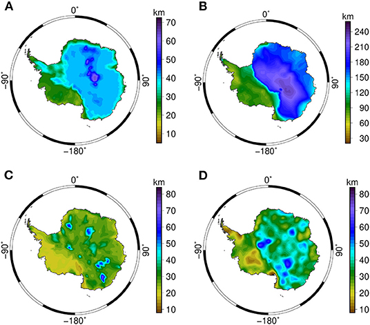
Figure 4. (A) Moho depth, (B) Lithosphere-asthenosphere boundary depth, (C) Curie isotherm depth from the seismologically inferred lithosphere model by An et al. (2015) and (D) the Curie isotherm depth derived from spectral magnetic analysis by Martos et al. (2017).
We use the AN1 model as reference case and then replace either the Moho or Curie isotherm depths in order to investigate the compatibility of the differently derived models and interdependencies between the inverted thermal parameters. Therefore, different Moho depths from the mostly seismic ANT model (Baranov and Morelli, 2013) and its updated version (Baranov et al., 2018), here referred to as “Baranov”; a global crustal model CRUST1.0 (Laske et al., 2013); a satellite gravity inversion “GravInv” (Pappa et al., 2019) and a Kriging interpolation from a global data compilation of active seismics (Szwillus et al., 2019) are used. Furthermore, we compare the seismological Curie isotherm from the AN1 model with the magnetically derived Curie from Martos et al. (2017), which is called “Martos” hereinafter for abbreviation (Figure S5A). It is noticeable that the Martos Curie is overall deeper than the AN1 Curie isotherm model in East Antarctica while it exhibits some extremely shallow structures in West Antarctica at the Ross Ice Shelf, Marie-Byrd-Land, and the Peninsula.
In addition, we use a map of predicted upper crustal heat production rates for the Antarctic Peninsula from geological information and geochemical analyses from Burton-Johnson et al. (2017) to explore the effect of heterogeneity of heat producing elements.
All these models were resampled on a uniform grid with a resolution of 50 by 50 km.
3. Results
3.1. AN1 Model
The thermal parameters (crustal heat production, mantle heat flux and thermal conductivity) obtained from inverting the seismological model AN1 reflect the pronounced partition between East and West Antarctica (Figure 5). The mantle heat flux (Figure 5D) as expected correlates strongly with the LAB depths and is around 10−20 mW/m2 in East Antarctica and above 30 mW/m2 in West Antarctica. A similar pattern is observed for crustal heat production, very low in East Antarctica, but more than 3.0μWm−3 in West Antarctica (Figure 5A), which correlates with the Moho depth (Figure 4A). For the thermal conductivity, the inversion results displays random fluctuations around the center of the prior range (Figures 5B,C). Both, heat production and the calculated GHF (Figure 5E) strongly resemble the Curie isotherm. In areas of deeper Curie depths down to 65 km the GHF is between 30 and 40 mW/m2 with low heat production below 1.0μWm−3. In shallower Curie depth regions between 15 and 20 km, like in Victoria Land along the Transantarctic Mountains, the GHF reaches up to 140 mW/m2 and exhibibts higher heat production rates around 6.0μWm−3.
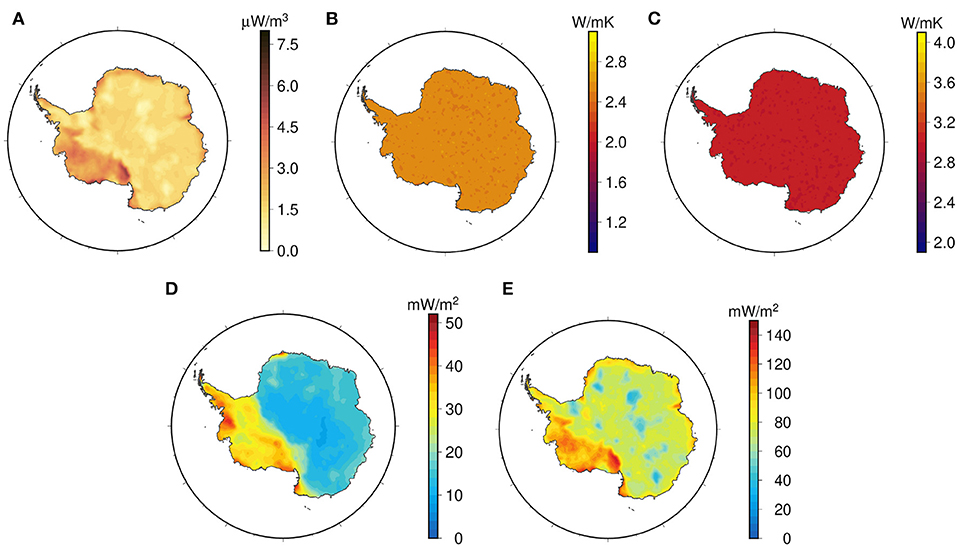
Figure 5. Thermal parameters from the probabilistic inversion of the AN1 model and the derived surface heat flux with 1, 000, 000 iterations per column. (A) Crustal heat production rates, (B) Crustal thermal conductivity, (C) Mantle thermal conductivity, (D) Mantle heat flux, (E) Surface heat flux.
The relations between the different parameters are visualized separately for the western (A) and eastern (B) part in Figure 6. Reciprocal correlations can be observed between heat production and Moho or Curie depth, as well as between GHF and Curie depth and between mantle heat flux and LAB, meaning that deeper lithospheric boundaries correlate with a decrease of heat flux and heat production. Additionally, there is a strong linear relation between heat production and GHF, which has been demonstrated empirically already by Roy et al. (1968). Other combinations show a rather minor or no correlation, e.g., crustal and mantle thermal conductivity. It is noticeable that the correlations for East Antarctica are thinned out with respect to West Antarctica, indicating that the eastern part is geologically more homogeneous and therefore more constrained. Likewise, the standard deviations of heat production and mantle heat flux are slightly higher in West Antarctica (Figures S2A,B). Especially in the region of the Ross Ice Shelf they reach values of about 1.2 μW/m3 and 5 mW/m2, respectively, where the depths of the AN1 model are notably shallow and the resulting GHF is high. The uncertainty of the GHF is therefore also higher in West Antarctica with values around 20 mW/m2, while indicating low values in the East around 5 mW/m2 (Figure S3A). Standard deviations of thermal conductivities (Figures S2C,D), as the parameters themselves, show no spatial dependence.
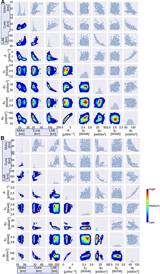
Figure 6. Correlations between different input (marked with blue rectangles) and output parameters resulting from the inversion with the AN1 model for (A) West and (B) East Antarctica. The lower triangles of both plots show the density of the parameter combinations. The frequency of each parameter is on the diagonal and the upper triangles show all inversion results as scattered dots.
The temperatures at the Curie and LAB isotherms are fitted relatively close to the specified values of 580 and 1, 315°C (Figures S4A,B) and deviations are about ±1°C at the Curie and ±2°C at the LAB isotherm. In particular, the region with a deeper crust, and a respectively thinner lithospheric mantle, which is also a complex region of transition between East and West Antarctica is slightly below the pre-defined LAB temperature. The mean σT (Figure S4C) is evenly scattered with values around 5.4 − 5.6°C as average of the allowed range from 1.0°C to 10.0°C. In this case, a temperature uncertainty of C would mean a maximum depth uncertainty of about σCurie = 1.5 km (with k2, max = 3.0 W/mK and qS, min = 20 mW/m2) and σLAB = 8 km (with k2, max = 4.0 W/mK and qD, min = 5 mW/m2).
3.2. Variation of Moho Depth
Seven different Moho depth models are tested (as described in section 2.4), while we constantly use the LAB and Curie depth of the AN1 model. We find that the Moho depth has an influence on the crustal heat production, i.e., a thin crust is compensated with higher rates of heat production (Figure 6). The relation between different Moho depths and GHF is visualized in Figure S5, which shows that the Moho can have an influence on the shape of the correlation, due to the different depth ranges of the distinct models. Though, the magnitude of the heat flux remains almost the same, with differences only up to 2 mW/m2 of the mean GHF. In general we do not see significant changes in the output of the thermal parameters by varying the Moho, suggesting that distinct methods and small uncertainties in determining this depth have no significant impact on our heat flux results.
3.3. Variation of Curie Isotherm
Here we investigate the influence of the model by Martos et al. (2017) (Figure 4D) in comparison to the seismological model from An et al. (2015) (Figure 4C) and additionally a Curie isotherm depth which is set equal to the Moho depth (with the Moho depth from AN1 Figure 4A).
The results of the inversion with the Martos Curie are shown in Figure 7. It is noticeable that the GHF is most affected by changing the Curie depth. It is overall lower, especially in East Antarctica, where it is almost homogeneously around 50 mW/m2. In West Antarctica we get distinct areas of higher GHF, correlating with shallow Curie depths, that reach up to 190 mW/m2 with strong contrasts to their surroundings. These areas also correspond to higher uncertainties of GHF around 30 mW/m2 (Figure S3B). The remaining inverted thermal parameters do not show significant differences from the AN1 results, besides slightly lower crustal conductivities and an anomaly in the region of the Transantarctic Mountains, where the Martos Curie is deeper than the AN1 Moho (Figure S6B) and the LAB is shallow.
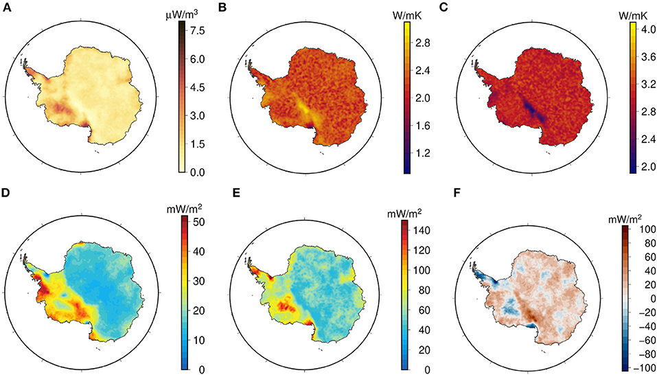
Figure 7. Thermal output parameters from the probabilistic inversion for the combination of the AN1 model with the magnetic Curie depth from Martos et al. (2017) and the subsequently calculated and residual GHF between both versions (AN1 - Martos). (A) Crustal heat production rates, (B) Crustal thermal conductivity, (C) Mantle thermal conductivity, (D) Mantle heat flux, (E) Surface heat flux, (F) Residual surface heat flux (AN1 model - AN1 model with Martos Curie).
The reciprocal correlation between the Curie depth and the GHF is noticeably different when we use the magnetically derived Curie depth (Figure 8). Furthermore, the density of the parameter combinations shows that the average AN1 Curie isotherm lies much shallower in about 25 km depth than the magnetically derived Curie isotherm, which mainly is around 40 km, equal to the median Moho depth from the AN1 model. Therefore, we only get minor differences by using either a Curie depth equal to the AN1 Moho (Figure 8B) or the Martos Curie (Figure 8C) with mean GHF of 63.08 mW/m2 and 68.78 mW/m2, respectively. A deeper Curie isotherm results in a significantly colder model with less radiogenic heat production and an incorrect determination can therefore have a strong and important impact on the results.
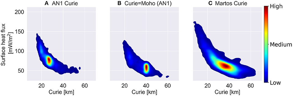
Figure 8. Density plot of Curie depths and surface heat fluxes for the AN1 model showing their anticorrelation for different Curie depths models. (A) AN1 model, (B) Curie is set equal to the Moho depth from the AN1 model and (C) with the Martos Curie isotherm which exhibits a noticeable aberration of the surface heat flux—Curie depth—correlation.
3.4. Influence of Heat Production
3.4.1. Exponential Decrease
A first approximation of more geologically realistic parameters is to assume that the heat production is not vertically constant but decreases exponentially (e.g., Lachenbruch, 1970). This approach preserves the observed linear relation between surface heat production and GHF as well as differential erosion at the surface (Lachenbruch, 1970; Turcotte and Schubert, 2014). The influence of the exponentially decreasing heat production on the inversion results is shown in Figure S8, indicating that much higher values, up to about 4 μW/m3, are needed in order to balance the depth decrease. Moreover, the crustal thermal conductivity features a clearer separation of East and West Antarctica with overall lower values of about 1.5 W/mK and 2.0 W/mK, respectively, and a stronger correlation with the Curie isotherm. The GHF shows the opposite and appears uncorrelated.
3.4.2. Spatial Variability
The correlations between the different thermal parameters in Figure 6 indicate a strong heterogeneity of West Antarctica and the considerable non-uniqueness was shown by the synthetic tests (section 2.3). Thus, more constraints are needed, which could be based on geological information. Heat production measurements can only be made at few locations where rock outcrops allow sampling. Here, we exploit the heat production map of the Antarctic Peninsula from Burton-Johnson et al. (2017) and use this as a constraint in the inversion. We fix the heat production to spatially varying surface values and thus one parameter less needs to be adjusted probabilistically.
This set-up leads to more pronounced patterns of the different thermal parameters. Figure 9 shows this for the GHF and crustal thermal conductivity with and without the geological constraints. As shown in section 2.3, the fixation of the heat production limits the ranges of the crustal thermal conductivity and thus, we get a different distribution that shows the correlation between these parameters. With these constraints (Figures 9B,E) we obtain clearly accentuated provinces with high GHF of about 110 mW/m2 and crustal thermal conductivities, about 3.5 W/mK, surrounded by lower values of approximately 70 mW/m2 and 1.5 W/mK. Overall we get lower GHF and higher crustal thermal conductivities with differences between both models that reach up to approximately ±80 mW/m2 and ±1.5 W/mK, respectively (Figures 9C,F). As expected, the spatial distribution of the thermal properties reflect the geological input from Burton-Johnson et al. (2017). In their study, Burton-Johnson et al. (2017) also used the AN1 model and the same parameter set-up (with a layered crust, see Table 1) as An et al. (2015) for the heat flux calculation, which is similar to our results.
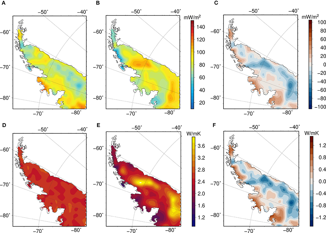
Figure 9. Surface heat flux (A–C) and crustal thermal conductivity (D–F) for the Antarctic Peninsula with the AN1 depth model. Left: with unconstrained heat production. Middle: with geologically constrained heat production values from Burton-Johnson et al. (2017). Right: residuals (without constraints—with heat production constraints).
4. Discussion
The MCMC approach gives reasonable results for the GHF that are comparable to previous studies without restricting the lateral variance of thermal conductivity, heat production and mantle heat flux. While the crustal and mantle conductivity could not be resolved well and only reproduce the mean of the assumed prior information, heat production and mantle heat flux show clear lateral variations depending on the input models for Curie, Moho, and LAB depth.
The spatial distribution of the GHF calculated with the AN1 model in this study has a similar spatial pattern as the original estimates (Figure 1D), but are overall higher by about 20 mW/m2 (see Figure S7A). In our analysis, the prior range of heat production values ranges from 0.0 to 7.0μWm−3, whereas An et al. (2015) used laterally constant and comparably low values that decrease step wise with depth (see Table 1). Likewise, their applied thermal conductivity is laterally constant but changes with depth depending on the temperature within the crust, while the inversion leads to values of about 2.5 W/mK for the crust and 3.0 W/mK for the mantle.
Similarly, the GHF calculated with the Martos Curie depth is comparable to the results from the study of Martos et al. (2017) (Figure 1E) although they used exponentially decreasing and laterally constant heat production rates with a surface value of H0 = 2.5μWm−3 and a reference depth of hr = 8 km. However, they assumed a constant crustal thermal conductivity of 2.8 W/mK which is only slightly higher than the inversion results which lie between 2.0 and 2.5 W/mK. Therefore the average residual heat flux between the inversion with the Martos Curie and the original study is only around ±5 mW/m2 (Figure S7B) indicating the strong influence of the Curie isotherm for the heat flux calculation.
Changing either the Moho or Curie depths has distinct impacts on the modeling of heat flux. The geometry of the Moho depth has a minor effect (Figure 10), hence the changes in thermal properties between crust and mantle play a secondary role. Yet, we see lower heat production rates in East Antarctica as a result of its correlation with the Moho and Curie depths. In fact, a colder and deeper crust implies a higher proportion of Archean rocks in East Antarctica, which have been shown to have a lower radiogenic content (e.g., Morgan, 1985 or Rudnick and Nyblade, 1999). Though this correlation might lead to a weakened relation between GHF and crustal thickness, which explains the comparatively small variations in GHF for different Moho depth models (Figure 10). Constraints on heat production from geological studies would help to reconcile this limitations of the inversion. In contrasts, the depth of the Curie isotherm has a significant influence on our modeled results. Thus, it would be important to determine this isotherm as accurately as possible.
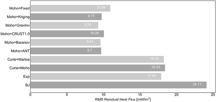
Figure 10. RMS residual surface heat flux between different tested model variations and the inverted AN1 model. Varying the Moho depth leads to slight but similar changes of the heat flux. The variation of the Curie depth and the exponential decreasing heat production (“Exp”) in contrast show significantly higher differences, whereas the geological constraints of Burton-Johnson et al. (2017) (“BJ”) indicate the highest deviation.
However, the seismological model does not consider variable mineralogy or water composition and the exact relation between velocity anomalies and temperature is unknown, hence the resulting Curie isotherm has a high uncertainty, which also holds for the magnetic approach. For example, the Curie depth from Martos et al. (2017) is over large areas deeper than the seismic Moho depth. It is generally accepted that the Moho boundary as a compositional boundary limits magnetization in depths (Wasilewski and Mayhew, 1992) and that the mantle contributes to a lesser degree. Therefore, the large magnetic Curie isotherm depths point a structural rather than a thermal source of the lateral changes (Frost and Shive, 1986; Wasilewski and Mayhew, 1992). Figure 10 shows that we get comparable results by either using a Curie depth equal to the AN1 Moho depth or the magnetic Curie depth. Both set-ups result in a residual heat flux of about 18 mW/m2 compared to the AN1 model. In our analysis, we showed that the combination of the seismological lithospheric model with the magnetically derived Curie depth, results in large differences. Especially in regions of a deep magnetic Curie depth and shallow seismic LAB, the models are not compatible. There, the temperature would increase rapidly over a short distance, requiring unrealistically high crustal and low mantle thermal conductivities. Changing the Curie depth leads to completely different GHF similar to the published results from An et al. (2015) and Martos et al. (2017), respectively. The spatial distribution of the GHF is mirrored by the Curie isotherm and in the case of the magnetic Curie we also get similar magnitudes.
However, we observe that a deep LAB in East Antarctica leads to more constrained mantle heat fluxes and heat production rates and thus, less scope for the inversion. In any case, the interplay between the lithospheric boundaries influences the inversion results considerably and consistent depth models would be beneficial. Note that this study does not intent to give new absolute heat flux estimations, but to give an overview of the consistency of some of the available Antarctic models and the interdependencies and importance of the different thermal parameters.
Different approaches for the heat production in our model show that this parameter has an essential influence on the magnitude and spatial distribution of GHF and thermal conductivity. Assuming exponentially decreasing heat production like Martos et al. (2017) and Fox Maule et al. (2005), leads to models of elevated rates at the surface with no more correlation to the Curie isotherm. In contrast, the crustal thermal conductivity is significantly lower and more correlated to the Curie. The resulting GHF is slightly lower and the separation between East and West Antarctica is less evident. For example, measurements of heat production of a suite of Proterozoic (1.2−2.0 Ga) granitoids sourced within the Byrd and Nimrod glacial drainages of central East Antarctica indicate average upper crustal heat production of about 2.6±1.9μWm−3 (Goodge, 2018). Such high values can easily be explained by an exponentially decreasing heat production in order to explain the generally low heat flux. However, the applicability of the exponential relationship is still under discussion as it has not been validated by direct measurements and may only apply to a systematically differentiated granitoid crust (Lachenbruch, 1970). A generally downward-decreasing, but laterally high variable heat production in the crust was shown to equally explain the linear correlation between heat production and GHF (e.g., Fountain et al., 1987; Kukkonen and Lahtinen, 2001). However, there is no simple heat production trend with depth that is consistent on a global scale due to perturbations by for example fluid circulation and/or magmatic activity (Ĉermák et al., 1991) and local crustal features need to be taken into account.
The strongest change of the GHF with respect to the AN1 model is obtained by introducing the geological constrained heat production rates from Burton-Johnson et al. (2017) with a difference of about 24 mW/m2 (Figure 10). We see more pronounced patterns of GHF and thermal conductivity in contrast to their irregular distribution by inverting for heat production without geological constraints (Figure 9). These substantial differences emphasize that laterally constant heat production values, as used by previous studies, are not appropriate and more geological information is required. Therefore, it would be important to get a well-defined heat production map for Antarctica.
In the case of Antarctica with a sparse knowledge about tectonics, composition, and heat flux, every indication of a more natural (and not apparently random or laterally constant) distribution of thermal parameters can be seen as an improvement. Pollett et al. (2019) interpreted measurements of GHF in a Gondwana framework by kriging interpolation. Such interpolation with sparse data points results in high uncertainties. We suggest instead to combine this approach with a definition of preliminary tectonic provinces as for example by multivariate analysis (e.g., Stål et al., 2019). In the combined set-up data from the formerly adjacent continents can be used as proxies to adjust our prior parameter ranges, at least to study GHF in East Antarctica. A continent-wide geological and geochemical database, e.g., from extrapolation of geological information from former adjacent continents like Africa, India and Australia, would be ideal in order to get meaningful heat flux models as important constraints for ice sheet modeling. In contrast to previous studies, the MCMC approach would still leave some freedom for lateral variance of the thermal parameters, while at the same time it would be geologically constrained. For West Antarctica, such an approach is not possible, but here one should make use of the wealth of geophysical high-resolution data acquired over the last years (e.g., Golynsky et al., 2018; Scheinert et al., 2016; Shen et al., 2018) and couple these in the analysis.
5. Conclusions
This paper gives an overview of the influences of different thermal parameters on the Antarctic GHF and presents a probabilistic approach which makes lateral variations for the Antarctic continent accessible. The Bayesian Monte-Carlo-Markov-Chain method gives horizontally variable heat production rates and mantle heat fluxes that correlate strongly with Curie depth and LAB, respectively. Both parameters get more constrained with deeper lithospheric structures so that East Antarctica exhibits lower uncertainties than West Antarctica. Geological information on the Antarctic Peninsula gives thoroughly different GHF results and helps to restrict the crustal thermal conductivity.
Data Availability Statement
Martos, Y. M. (2017): Antarctic geothermal heat flux distribution and estimated Curie Depths, links to gridded files. PANGAEA, https://doi.org/10.1594/PANGAEA.882503, Supplement to: Martos et al. (2017).
An, M. and Feng, M. (2015): http://www.seismolab.org/, Supplement to: An et al. (2015).
Burton-Johnson, A., Halpin, J. A., Whittaker, J. M., Graham, F. S., and Watson, S. J. (2017): https://doi.org/10.1002/2017GL073596, Supplement to: Burton-Johnson et al. (2017).
The inversion code can be found on GitHub.
Author Contributions
ML drafted the manuscript and performed all calculations. JE contributed to the conception of the study. WS wrote sections 2.1 and 2.2 of the manuscript and the inversion code. All authors contributed to manuscript revision, read and approved the submitted version.
Funding
This work was supported by the Deutsche Forschungsgemeinschaft (DFG) in the framework of the priority programme Antarctic Research with comparative investigations in Arctic ice areas by a grant (Grant No. EB 255/8-1).
Conflict of Interest
The authors declare that the research was conducted in the absence of any commercial or financial relationships that could be construed as a potential conflict of interest.
Supplementary Material
The Supplementary Material for this article can be found online at: https://www.frontiersin.org/articles/10.3389/feart.2020.00105/full#supplementary-material
References
Ĉermák, V., Bodri, L., and Rybach, L. (1991). Terrestrial heat flow and the lithosphere structure,? in Exploration of the Deep Continental Crust, eds V. Ĉermák and L. Rybach (Berlin; Heidelberg: Springer-Verlag), 23–69.
Afonso, J., Fullea, J. C., Griffin, W. L., Yang, Y., Jones, A. G., Connolly, J. A. D., et al. (2013). 3-D multiobservable probabilistic inversion for the compositional and thermal structure of the lithosphere and upper mantle. I: a priori petrological information and geophysical observables. J. Geophys. Res. Solid Earth 118, 2586–2617. doi: 10.1002/jgrb.50124
An, M., Wiens, D. A., Zhao, Y., Feng, M., Nyblade, A., Kanao, M., et al. (2015). Temperature, lithosphere-asthenosphere boundary, and heat flux beneath the Antarctic plate inferred from seismic velocities. J. Geophys. Res. Solid Earth 120, 8720–8742. doi: 10.1002/2015JB011917
Baranov, A., and Morelli, A. (2013). The moho depth map of the Antarctica region. Tectonophysics 609, 299–313. doi: 10.1016/j.tecto.2012.12.023
Baranov, A., Tenzer, R., and Bagherbandi, M. (2018). The moho depth map of the Antarctica region. Surv. Geophys. 39, 23–56. doi: 10.1007/s10712-017-9423-5
Bell, R. E. (2008). The role of subglacial water in ice-sheet mass balance. Nat. Geosci. 1, 297–304. doi: 10.1038/ngeo186
Bodin, T., Sambridge, M., Tkalcić, H., Gallagher, K., and Rawlinson, N. (2012). Transdimensional inversion of receiver functions and surface wave dispersion. J. Geophys. Res. 117:B02301. doi: 10.1029/2011JB008560
Burton-Johnson, A., Halpin, J. A., Whittaker, J. M., Graham, F. S., and Watson, S. J. (2017). A new heat flux model for the Antarctic peninsula incorporating spatially variable upper crustal radiogenic heat production. Geophys. Res. Lett. 44, 5436–5446. doi: 10.1002/2017GL073596
Decker, E. R., and Bucher, G. J. (1982). Geothermal Studies in the Ross Island-Dry Vally Region, Vol. 4. Madison, WI: University of Wisconsin Press.
Engelhardt, H. (2004). Ice temperature and high geothermal flux at Siple Dome, west Antarctica, from borehole measurements. J. Glaciol. 50, 251–256. doi: 10.3189/172756504781830105
Fisher, A. T., Mankoff, K. D., Tulaczyk, S. M., Tyler, S. W., Foley, N., and the WISSARD Science Team (2015). High geothermal heat flux measured below the west Antarctic ice sheet. Am. Assoc. Adv. Sci. 1, 2375–2548. doi: 10.1126/sciadv.1500093
Fountain, D. M., Salisbury, M. H., and Furlong, K. P. (1987). Heat production model of a shield area and its implications for the heat flow - heat production relationship. Geophys. Res. Lett. 14, 283–286. doi: 10.1029/GL014i003p00283
Fox Maule, C., Purucker, M. E., Olsen, N., and Mosegaard, K. (2005). Heat flux anomalies in Antarctica revealed by satellite magnetic data. Science 309, 464–467. doi: 10.1126/science.1106888
Frost, B. R., and Shive, P. N. (1986). Magnetic mineralogy of the lower continental crust. J. Geophys. Res. 91, 6513–6521. doi: 10.1029/JB091iB06p06513
Golynsky, A. V., Ferraccioli, F., Hong, J. K., Golynsky, D. A., von Frese, R. R. B., Young, D. A., et al. (2018). New magnetic anomaly map of the Antarctic. Geophys. Res. Lett. 45, 6437–6449. doi: 10.1029/2018GL078153
Goodge, J. W. (2018). Crustal heat production and estimate of terrestrial heat flow in central east Antarctica, with implications for thermal input to the east Antarctic ice sheet. Cryosphere 12, 491–504. doi: 10.5194/tc-12-491-2018
Kukkonen, I. T., and Lahtinen, R. (2001). Variation of radiogenic heat production rate in 2.8-1.8 ga old rocks in the central Fennoscandian shield. Phys. Earth Planet. Interiors 126, 279–294. doi: 10.1016/S0031-9201(01)00261-8
Lachenbruch, A. H. (1970). Crustal temperature and heat production: implications of the linear heat-flow relation. J. Geophys. Res. 75, 3291–3300. doi: 10.1029/JB075i017p03291
Larour, E., Seroussi, H., Morlighem, M., and Rignot, E. (2012). Continental scale, high order, high spatial resolution, ice sheet modeling using the ice sheet system model (ISSM). J. Geophys. Res. 117:F01022. doi: 10.1029/2011JF002140
Laske, G., Masters, G., Ma, Z., and Pasyanos, M. (2013). Update on crust1.0 - a 1-degree global model of Earth's crust. Geophys. Res. Abstracts 15:2658. Available online at: http://igppweb.ucsd.edu/~gabi/rem.html
Llubes, M., Lanseau, C., and Rémy, F. (2013). Relations between basal conditions, subglacial hydrological networks and geothermal flux in Antarctica. Earth Planet. Sci. Lett. 241, 655–662. doi: 10.1016/j.epsl.2005.10.040
Martos, Y. M., Catalán, M., Jordan, T. A., Golynsky, A., Golynsky, D., Eagles, G., et al. (2017). Heat flux distribution of Antarctica unveiled. Geophys. Res. Lett. 44, 11417–11426. doi: 10.1002/2017GL075609
Morgan, P. (1985). Crustal radiogenic heat production and the selective survival of ancient continental crust. J. Geophys. Res. 90, C561?C570. doi: 10.1029/JB090iS02p0C561
Morin, R. H., Williams, T., Henrys, S. A., Magens, D., Niessen, F., and Hansaraj, D. (2010). Heat flow and hydrologic characteristics at the and-1b borehole, andrill mcmurdo ice shelf project, Antarctica. Geosphere 6, 370–378. doi: 10.1130/GES00512.1
Pappa, F., Ebbing, J., and Ferraccioli, F. (2019). Moho depths of antarctica: Comparison of seismic, gravity, and isostatic results. Geochem. Geophys. Geosyst. 20, 1629–1645. doi: 10.1029/2018GC008111
Pollack, H. N., Hurter, S. J., and Johnson, J. R. (1993). Heat flow from the earth's interior: analysis of the global data set. Rev. Geophys. 31, 267–280. doi: 10.1029/93RG01249
Pollett, A., Hasterok, D., Raimondo, T., Halpin, J. A., Hand, M., Bendall, B., et al. (2019). Heat flow in southern Australia and connections with east Antarctica. Geochem. Geophys. Geosyst. 20:2019GC008418. doi: 10.1029/2019GC008418
Purucker, M. E., Langel, R. A., Rajaram, M., and Raymond, C. (1998). Global magnetization models with a priori information. J. Geophys. Res. Solid Earth 103, 2563–2584. doi: 10.1029/97JB02935
Ravat, D., Pignatelli, A., Nicolosi, I., and Chiappini, M. (2007). A study of spectral methods of estimating the depth to the bottom of magnetic sources from near-surface magnetic anomaly data. Geophys. J. Int. 169, 421–434. doi: 10.1111/j.1365-246X.2007.03305.x
Risk, G. F., and Hochstein, M. P. (1974). Heat flow at arrival heights, Ross island, Antarctica. N. Z. J. Geol. Geophys. 17, 629–644. doi: 10.1080/00288306.1973.10421586
Roy, R. F., Blackwell, D. D., and Birch, F. (1968). Heat generation of plutonic rocks and continental heat flow provinces. Earth Planet. Sci. Lett. 5, 1–12. doi: 10.1016/S0012-821X(68)80002-0
Rudnick, R. L., and Nyblade, A. A. (1999). The thickness and heat production of Archean lithosphere: constraints from xenolith thermobarometry and surface heat flow. Mantle Petrol. 6, 3–12.
Scheinert, M., Ferraccioli, F., Schwabe, J., Bell, R., Studinger, M., Damaske, D., et al. (2016). New Antarctic gravity anomaly grid for enhanced geodetic and geophysical studies in Antarctica. Geophys. Res. Lett. 43, 600–610. doi: 10.1002/2015GL067439
Schroeder, H., Paulsen, T., and Wonik, T. (2011). Thermal properties of the and-2a borehole in the southern Victoria land basin, Mcmurdo sound, Antarctica. Geosphere 7, 1324–1330. doi: 10.1130/GES00690.1
Shen, W., Wiens, D. A., Anandakrishnan, S., Aster, R. C., Gerstoft, P., Bromirski, P. D., et al. (2018). The crust and upper mantle structure of central and west Antarctica from Bayesian inversion of Rayleigh wave and receiver functions. J. Geophys. Res. Solid Earth 123, 7824–7849. doi: 10.1029/2017JB015346
Spector, A., and Grant, F. S. (1970). Statistical model for interpreting aeromagnetic data. Geophysics 35, 293–302. doi: 10.1190/1.1440092
Stål, T., Reading, A. M., Halpin, J. A., and Whittaker, J. M. (2019). A multivariate approach for mapping lithospheric domain boundaries in east Antarctica. Geophys. Res. Lett. 46, 10404–10416. doi: 10.1029/2019GL083453
Szwillus, W., Afonso, J. C., Ebbing, J., and Mooney, W. D. (2019). Global crustal thickness and velocity structure from geostatistical analysis of seismic data. J. Geophys. Res. Solid Earth 124, 1626–1652. doi: 10.1029/2018JB016593
Turcotte, D., and Schubert, G. (2014). Geodynamics, 3rd Edn. Cambridge, UK: Cambridge University Press. doi: 10.1017/CBO9780511843877
Van Liefferinge, B. (2018). Thermal state uncertainty assessment of glaciers and ice sheets: Detecting promising Oldest Ice sites in Antarctica (dissertation). Free University of Brussels, Brussels, Belgium.
Keywords: heat flux, Bayesian inversion, Monte-Carlo, numerical modeling, Antarctica
Citation: Lösing M, Ebbing J and Szwillus W (2020) Geothermal Heat Flux in Antarctica: Assessing Models and Observations by Bayesian Inversion. Front. Earth Sci. 8:105. doi: 10.3389/feart.2020.00105
Received: 22 January 2020; Accepted: 23 March 2020;
Published: 21 April 2020.
Edited by:
Pier Paolo Bruno, University of Naples Federico II, ItalyReviewed by:
Tom Aldo Jordan, British Antarctic Survey (BAS), United KingdomYasmina M. Martos, Goddard Space Flight Center (NASA), United States
Copyright © 2020 Lösing, Ebbing and Szwillus. This is an open-access article distributed under the terms of the Creative Commons Attribution License (CC BY). The use, distribution or reproduction in other forums is permitted, provided the original author(s) and the copyright owner(s) are credited and that the original publication in this journal is cited, in accordance with accepted academic practice. No use, distribution or reproduction is permitted which does not comply with these terms.
*Correspondence: Mareen Lösing, bWFyZWVuLmxvZXNpbmcmI3gwMDA0MDtpZmcudW5pLWtpZWwuZGU=