Calculation of the Vertical Velocity in the Asian Summer Monsoon Anticyclone Region Using the Thermodynamic Method With in situ and Satellite Data

Correctly calculating the vertical velocity of the Asian summer monsoon anticyclone (ASMA) region is helpful for accurately knowing the ozone stratosphere–troposphere exchange, so as to explore the variation of ozone in the ASMA region. Therefore, the vertical velocity over the ASMA in June, July, August, and September 2012 and 2016 was calculated using the thermodynamic method, which may avoid the deviations produced by the kinematics method using the mass continuity equation. In order to improve the accuracy, we used high-resolution heating rate datasets obtained via the radiation model in Canadian Atmospheric Global Climate Model called CanAM4.3_RAD based on in situ observations and revised satellite data from MLS/AIRS. The vertical velocity calculated by the thermodynamic method (V_T) is then compared with the data from ERA-Interim (V_ERA–I). In the daytime, values of V_T were similar to V_ERA–I and were dominated by ascending motion, although V_T showed descending motion at the western edge of the ASMA below 100 hPa. The intensity of V_T was slightly smaller than that of V_ERA–I at lower levels (200–100 hPa) over the ASMA region and significantly weaker above 100 hPa. The situation was more complex at night. Both V_T and V_ERA–I showed the convergence of vertical wind at 150 hPa and the divergence at 80 hPa, but V_T had a smaller standard deviation. V_T showed descending in the western and northern ASMA, but V_ERA–I only descended in the west. The descending motion in the west, seen in both V_T and V_ERA–I, is produced by the heating difference between the Qinghai–Tibet Plateau and the Iranian Plateau. The difference of the two vertical velocities in the northern ASMA may indicate the different understandings of the local Hadley Circulation and local Brewer-Dobson Circulation.

Introduction

About ∼99% of all weather phenomena occur in the troposphere, but the stratosphere, which accounts for ∼15% of the total mass of the Earth’s atmosphere, has an important role in atmospheric studies (Holton, 1990; Dessler and Sherwood, 2004; Aschmann et al., 2009; Bian, 2009; Randel and Jensen, 2013; Zhang et al., 2016). Ozone is mainly present in the ozone layer, about 20 km above the Earth’s surface in the stratosphere (Lv et al., 2009; London and Park, 2011; Newman, 2014). The ozone layer absorbs ultraviolet radiation from the Sun and protects the surface biosphere from damaging radiation. Atmospheric fluctuations in the troposphere are uploaded to the stratosphere (Shepherd, 2002; Xie et al., 2012; He et al., 2020a, b; Yu et al., 2020), leading to the abnormal distribution of ozone in the stratosphere (Chen et al., 2019) and affecting the Earth’s climate (Bian et al., 2013; Lu and Ding, 2013; Xie et al., 2016; Li et al., 2017). Some anthropogenic ozone-depleting substances (ODSs), such as chlorofluorocarbons (CFCs) and halons, may also be transported to the stratosphere and influence the stratospheric ozone, while stratospheric ozone may transport to the troposphere and influence the tropospheric ozone (Elliot and Rowland, 1987; Schauffler et al., 1999; Butchart and Scaife, 2001; Newman et al., 2009; Oram et al., 2017; Wang et al., 2019, 2020). Research on stratosphere–troposphere exchange is therefore important in studying stratospheric ozone evolution (Liu et al., 2003; Tian et al., 2008; Bian et al., 2011a, 2020; Guo et al., 2012, 2015, 2017; Xie et al., 2012; Pavlov et al., 2013; Zhang H. et al., 2014; Gerber, 2015; Zhang J. et al., 2018). Previous studies have determined the structural distribution, vertical transport, and dynamics (Antokhin and Belan, 2013) of ozone in the stratosphere via LiDAR measurements (Kuang et al., 2012; Pavlov et al., 2013) the inversion of occultation data (Sofieva et al., 2017) and numerical simulations (Yang et al., 2004; Considine et al., 2008).

The Qinghai–Tibet Plateau, with an altitude of about 4,000 m, has an important role in global stratospheric–tropospheric exchange (Liu, 1998, 2007; Fu et al., 2006; Fan et al., 2008; Bian et al., 2011b, 2020; Tian et al., 2017). More research is required into upward transport over the Qinghai–Tibet Plateau as this is the most representative component of ozone in stratospheric–tropospheric exchange (Vaughan et al., 1994; Holton et al., 1995; Lv et al., 2009). The Asian summer monsoon anticyclone (ASMA) region, a stable high-pressure system over the Qinghai–Tibet Plateau in the summer, is the most important region of stratosphere–troposphere exchange (Zhou et al., 1995a; Cong et al., 2001; Chen et al., 2010; Deng et al., 2015; Fan et al., 2017a, b; Li et al., 2017, 2005; Yu et al., 2017; Shi et al., 2018; Yan et al., 2019) and accounts for almost 75% of this exchange process (Rosenlof, 1995; Stohl et al., 2003; Hu et al., 2009; Tian et al., 2009). Because of its existence, the structure and variation of ozone concentrations in the Qinghai–Tibet Plateau region are significantly different from the global average (Zhou and Luo, 1994; Zhou et al., 1995b; Zou and Gao, 1997; Zheng et al., 1998; Gettelman et al., 2004; Park et al., 2007; Vernier et al., 2009; Tang et al., 2019). Using satellite observations, Randel et al. (2010) confirmed that the ASMA region is an important channel for the mass transport from the troposphere to the stratosphere in summer. Ploeger et al. (2010) found that the timescales, paths, and diffusion of the mass flux are mainly determined by vertical transport. Bergman et al. (2012) proved that this vertical transport mainly relies on the vertical motion caused by the deviation of large-scale horizontal circulation over the ASMA region. Therefore, accurate calculations of the vertical velocity over the ASMA region are required to accurately estimate the transport of ozone.

The reliable calculation of the vertical velocity is a longstanding issue in numerical weather prediction (Krishnamurti and Bounoua, 1996). The vertical velocity is typically inferred from the mass continuity equation, which has been called the kinematics method by previous researchers (Eluszkiewicz et al., 2000; Mahowald et al., 2002; Schoeberl et al., 2003; Chipperfield, 2006). This method has a more simplified form (Cong et al., 2001; Gettelman et al., 2004; Chen et al., 2010; Zhan and Li, 2012). Sherman (1953) estimated the vertical velocity using the vertical equation and Lord and Jacqueline (1988), Uma and Rao (2009), Ploeger et al. (2010), and de Roode et al. (2012) assessed the impact of the vertical velocity scheme on the modeling of transport. Davis et al. (2007) used Doppler radar to estimate the mean vertical velocity of air.

The magnitude of the horizontal divergence is partially canceled in the ASMA region as a result of the opposite signs of the zonal and meridional divergence of the horizontal and vertical winds (Guo et al., 2012) and the divergence is insensitive to small perturbations in the large-scale horizontal circulation (Rex et al., 2008; Ploeger et al., 2010). Therefore, the deviations in calculating the divergence by the kinematic method will be carried over. The thermodynamic method has been used to avoid deviations from the kinematic method in the upper troposphere and lower stratosphere (UTLS) (Kistler et al., 2001; Rex et al., 2008; Ploeger et al., 2010). This method uses the diabatic heating rate to reflect the vertical motion of the atmosphere across the isentropic (θ) surface, and the vertical velocity is determined in a θ coordinate system (Rosenlof, 1995; Eluszkiewicz et al., 1996; Randel et al., 2002; Fueglistaler et al., 2005; Rex et al., 2008). Bergman et al. (2013) showed that numerical solutions are affected by the accuracy and resolution of the heating rates in the thermodynamic method. Some researchers have used satellite data and assimilation datasets to calculate heating rates (Rosenlof, 1995; Eluszkiewicz et al., 1996; Randel et al., 2002) and the results were clearly different (Liu et al., 2003; Yang et al., 2004).

Although some studies have applied the thermodynamic method, there is a lack of such research in the ASMA region. We used the revised satellite detection data from the microwave limb sounder (MLS) and the atmospheric infrared sounder (AIRS) for 2012 and 2016 reported by Shi et al. (2017) and the radiation model in Canadian Atmospheric Global Climate Model called CanAM4.3_RAD (Appendix A) to calculate the heating rate. We then applied the thermodynamic equation (Zhou et al., 2014) in isentropic coordinates to introduce a method to calculate the vertical velocity over the ASMA region.

Section “Materials and Methods” of this paper presents the data and methodology. Section “Results” compares the thermodynamic vertical velocity with the reanalysis data in different ways. We discuss the possible reasons for the deviations and the potential factors influencing the results in section “Discussion and Conclusions.”

Materials and Methods

Data

ERA-Interim Reanalysis Data

The ERA-Interim (ERA-I) reanalysis dataset has a higher credibility in the Qinghai–Tibet Plateau region than other reanalysis datasets, especially in the UTLS region, and realizes a more accurate description of the interannual variability (Monge-Sanz et al., 2007; Hu et al., 2009; Guo et al., 2017; Huang et al., 2018; Shi et al., 2018). The vertical velocity in the ERA-I dataset has previously been used as the kinematic vertical velocity in this region. We downloaded the ERA-I data directly from the European Centre for Medium-Range Weather Forecasts’ website¹, including the horizontal wind (u, v), vertical velocity (ω), and temperature (T) fields. The u, v, T, and p were used to determine the vertical velocity by thermodynamic method, and the ω was compared with the vertical velocity we calculated. The vertical resolution in the isobaric surfaces is 13 layers from 300 to 10 hPa. The horizontal grid resolution is 0.75° × 0.75° and the temporal resolution is 12 h. We used the dataset for the time period June, July, August, and September (JJAS) in 2012 and 2016.

Heating Rate Data

We substituted the heating rate with only the radiative heating rate data and ignored the sensible heat and latent heat. This is because the water vapor phase transition over the ASMA region is not significant as a result of the small amount of water vapor present and the low temperatures. The exchange of sensible heat is weak due to the small vertical temperature lapse rate and convection in the UTLS region. We used the CanAM4.3_RAD developed by Salzen et al. (2013) to calculate the radiative heating rate. This model can provide a high-accuracy simulation of the cloud radiation effect and the Earth’s radiation system (Zhang et al., 2013). The concentration of ozone, the temperature, and the water vapor content were required to drive the model and these data were obtained from the in situ observational profile of Ali station and the revised satellite dataset from MLS/AIRS.

The Ali dataset was obtained using a balloon-borne electrochemical concentration cell sonde at the Indus River (32.5°N, 80°E) in the central region of the ASMA. The electrochemical concentration cell measured the profiles with an accuracy within 10% in the troposphere and 5% in the stratosphere (Shi et al., 2017). The sounding balloons were launched at midnight from June to September 2016 to an altitude of 30 km. A total of 17 valid ozone profiles were obtained. In order to reduce the deviation taken by the time, human operation, and weather process, the JJAS average of Ali data was used to represent the summer mean.

The revised satellite dataset from the MLS/AIRS was corrected using the Ali dataset based on the MLS Level 2 Version 4 and the AIRS Version 6 Level 2 (L2) Support by different methods in JJAS 2012 and 2016. The original AIRS data had 55 layers from 515 to 10 hPa, and the original MLS data had 33 layers in total from upper troposphere to 0.1 hPa in the vertical direction (Yan et al., 2015; Gamelin and Carvalho, 2017; Herman et al., 2017; Shi et al., 2017). According to the spatial and temporal characteristics of the two data themselves, MLS was observed only in the longitudinal direction, along the horizontal plane of the flight path, while AIRS was observed in both the latitudinal and longitudinal directions, so we processed the MLS/AIRS into different analytical data. In the center of ASMA (about 25°N–42°N, 40°E–100°E), MLS and AIRS were revised by subtracting the summer mean deviation profile of Ali, and in the other area of ASMA, data were corrected by subtracting the half of the summer mean deviation profile of Ali (Shi et al., 2017). Their horizontal resolutions were 1.9° × 2.5° and 1° × 1°, respectively. In this way, we obtained the average heating rate at station Ali in JJAS 2016, the mean semi-monthly MLS heating rate, and the daily AIRS heating rate in JJAS 2012 and 2016.

Data Processing

The heating rate and ERA-I reanalysis data were interpolated in the horizontal and vertical directions to obtain the same temporal and spatial resolution before carrying out our calculations. We used typical linear interpolation for u, v, T, ω in the ERA-Interim dataset in the new horizontal grids of 1.9° × 2.5° and 1° × 1°, which are consistent with the MLS and AIRS heating rate data. We then interpolated the ERA-Interim data and the heating rate data into the same isentropic layers in the vertical direction. The layers were selected based on a combination of the vertical resolution between the two datasets. In this way, the resolution advantage of each dataset was preserved. The area was limited to (23°N–39°N, 70°E–107°E).

Methods

Calculation of Vertical Velocity

Previous studies (Eluszkiewicz et al., 2000; Mahowald et al., 2002; Schoeberl et al., 2003; Chipperfield, 2006) have shown that the vertical velocity can be determined using the kinematics equation in isobaric coordinates:

$$\mathrm{\omega }={\int }_{p1}^{p0}\left(\frac{\partial u}{\partial x}+\frac{\partial v}{\partial y}\right)\text{d}p(1)$$

which indicates that ω mainly depends on changes in the divergence term $\frac{\partial u}{\partial x}+\frac{\partial v}{\partial y}$. However, the term $\frac{\partial u}{\partial x}+\frac{\partial v}{\partial y}$ is insensitive to small perturbations in u and v and deviations from the observational data are common. We therefore applied the isentropic (θ) coordinate system:

$$\mathrm{\omega }={\left({\displaystyle \frac{\text{d}p}{\text{d}t}}\right)}_{\mathrm{\theta }}(2)$$

$$\mathrm{\omega }={\left({\displaystyle \frac{\text{d}p}{\text{d}t}}\right)}_{\mathrm{\theta }}={\left({\displaystyle \frac{\partial p}{\partial t}}\right)}_{\mathrm{\theta }}+{\left(\overrightarrow{V}\cdot \nabla p\right)}_{\mathrm{\theta }}(3)$$

$$\mathrm{\omega }={\left({\displaystyle \frac{\partial p}{\partial t}}\right)}_{\mathrm{\theta }}+{\left(u{\displaystyle \frac{\partial p}{\partial x}}+v{\displaystyle \frac{\partial p}{\partial y}}+{\mathrm{\omega }}_{\mathrm{\theta }}{\displaystyle \frac{\partial p}{\partial \mathrm{\theta }}}\right)}_{\mathrm{\theta }}(4)$$

Eq. 2 gives a method to determine the vertical wind by directly solving the pressure change rate in the isentropic coordinate system. This is then expanded in θ-coordinates in Eqs 3 and 4.

ω_θ is the vertical wind in θ-coordinates:

$${\mathrm{\omega }}_{\mathrm{\theta }}=\frac{\text{d}\mathrm{\theta }}{\text{d}t}(5)$$

The general form of the thermodynamic energy equation gives:

$$c_P\frac{\text{d}T}{\text{d}t}+p\frac{\text{d}\mathrm{\alpha }}{\text{d}t}=\stackrel{.}{Q}(6)$$

where $\stackrel{.}{Q}$ (J s^–1) is the diabatic heating rate, which means the change of adiabatic heating over time, c_P = 1,000 J/K⋅kg, is the specific heat at constant pressure, T (K) is the temperature, and p (Pa) is the atmosphere pressure.

Logarithmic differentiation of the potential temperature equation $\mathrm{\theta }=T{\left(\frac{P0}{P}\right)}^{R/Cp}$ gives

$$c_P\text{d}\ln \mathrm{\theta }=c_P\text{d}\ln \text{T-Rd}\ln p(7)$$

where R is the gas constant.

Combine Eq. 7 with Eq. 6 and let s = c_Pln⁡θ, so that the thermodynamic equation can be written as

$$\frac{\text{d}s}{\text{d}t}=\frac{\stackrel{.}{Q}}{T}(8)$$

Transforming this with θ gives

$$\frac{\text{d}\mathrm{\theta }}{\text{d}t}=\frac{\stackrel{.}{q}}{T}(9)$$

where $\stackrel{.}{q}=\frac{\text{d}\stackrel{\_}{Q}}{\text{d}t}=\frac{\mathrm{\theta }}{C_{\text{P}}}\stackrel{.}{Q}$.

Substituting Eq. 9 into Eq. 4, the diagnostic equation for the vertical velocity in isentropic coordinate system is obtained:

$$\mathrm{\omega }={\left(\frac{\partial p}{\partial t}\right)}_{\mathrm{\theta }}+{\left(u\frac{\partial P}{\partial x}+v\frac{\partial P}{\partial y}\right)}_{\mathrm{\theta }}+\frac{\partial P}{\partial \mathrm{\theta }}\frac{\mathrm{\theta }}{T\cdot C_P}\stackrel{.}{Q}(10)$$

The first term on the right-hand side is the local pressure tendency term, which represents the vertical velocity caused by the isentropic surface moving up and down locally. The second is the airflow advection term along the isentropic surface, which can be used to judge the direction of vertical velocity when the air flows from high to low pressure, producing an ascending motion and vice versa. The last diabatic term indicates that because $\frac{\partial P}{\partial \mathrm{\theta }}<0$, there is ascending motion when there is diabatic heating $(\stackrel{.}{Q}>0)$ and descending motion when there is diabatic cooling $(\stackrel{.}{Q}<0)$ (Zhou et al., 2014).

Statistical Analysis

We introduced some statistical variables for quantitative analysis (Rodgers, 1990; Von Clarmann, 2006; Shi et al., 2017):

$$\mathrm{\sigma }=\sqrt{{\displaystyle \frac{{\sum }_{i=1}^n{\left(V_i-\overline{V}\right)}^2}{n}}}(11)$$

$$b={\displaystyle \frac{{\sum }_{i=1}^n[V_{\text{AIRS}}(i)-V_{\mathrm{ERA}-\mathrm{I}}(i)]}{n}}(12)$$

$$\text{se}=\sqrt{{\displaystyle \frac{{\sum }_{i=1}^n{[(V_{\text{AIRS}}(i)-V_{\mathrm{ERA}-\mathrm{I}}(i))-b]}^2}{n(n-1)}}}(13)$$

Eq. 11 is the standard deviation (σ) of a variable where V_i is one of the vertical velocity values, the subscript i indicates the different times, and $\overline{V}$ is the mean value. This variable can illustrate the degree of discretization of each vertical velocity. The mean bias (b) in Eq. 12 was applied to describe the degree of deviation between the vertical velocity of the AIRS and ERA-I data. The standard error (se) is used in Eq. 13 to reduce the inaccuracy caused by abnormal or accidental conditions in Eq. 12. It is stipulated that when the interval (b - se, b + se) does not contain the value 0, then the difference between the two datasets described by b will be accepted and the result is considered to be statistically significant.

Results

Substituting three different heating rates into Eq. 10, we calculated the average vertical velocity profiles for Ali station in JJAS (V_Ali), the daily vertical velocity data of the AIRS (V_AIRS), and the monthly average vertical velocity of the MLS (V_MLS). We then compared these results with the vertical velocity in the ERA-Interim (V_ERA–I) dataset, which had been interpolated at the same spatiotemporal resolution. We used V_Ali, V_AIRS, and V_ERA–I to analyze the results for Ali station. We compared V_MLS with V_ERA–I for the ASMA region distribution analysis.

Results for Ali Station

Figure 1 shows the profiles of the nighttime vertical velocity at Ali station. It can be seen that V_Ali and V_ERA–I had a similar tendency, with a decreasing rate with height below 150 hPa, between 70 and 50 hPa, and an increasing rate with height in the other layers. In terms of the absolute values, the values in V_Ali and V_ERA–I approach each other below 80 hPa, but are different above 80 hPa. To make the difference clearer, we reduced the range of abscissa in (-0.1 to 0.4) in Figure 1A. V_ERA shows weaker ascending motion in the range of 70-50 hPa than that below 80 hPa, while V_Ali is mainly concentrated near the zero line, indicating insignificant vertical movement in the upper levels. They both indicate the vertical motions in the lower stratosphere (70-50 hPa) is weaker. For two vertical velocities, the wind reversed from ascending to descending around 200 hPa and the intensity of descending motion decreased gradually with increasing height. The vertical velocity reached zero near 80 hPa and the wind direction reversed again to a dominant ascending movement. The characteristics of low convergence and high divergence over the Qinghai–Tibet Plateau are described simultaneously by these two vertical velocities.

FIGURE 1

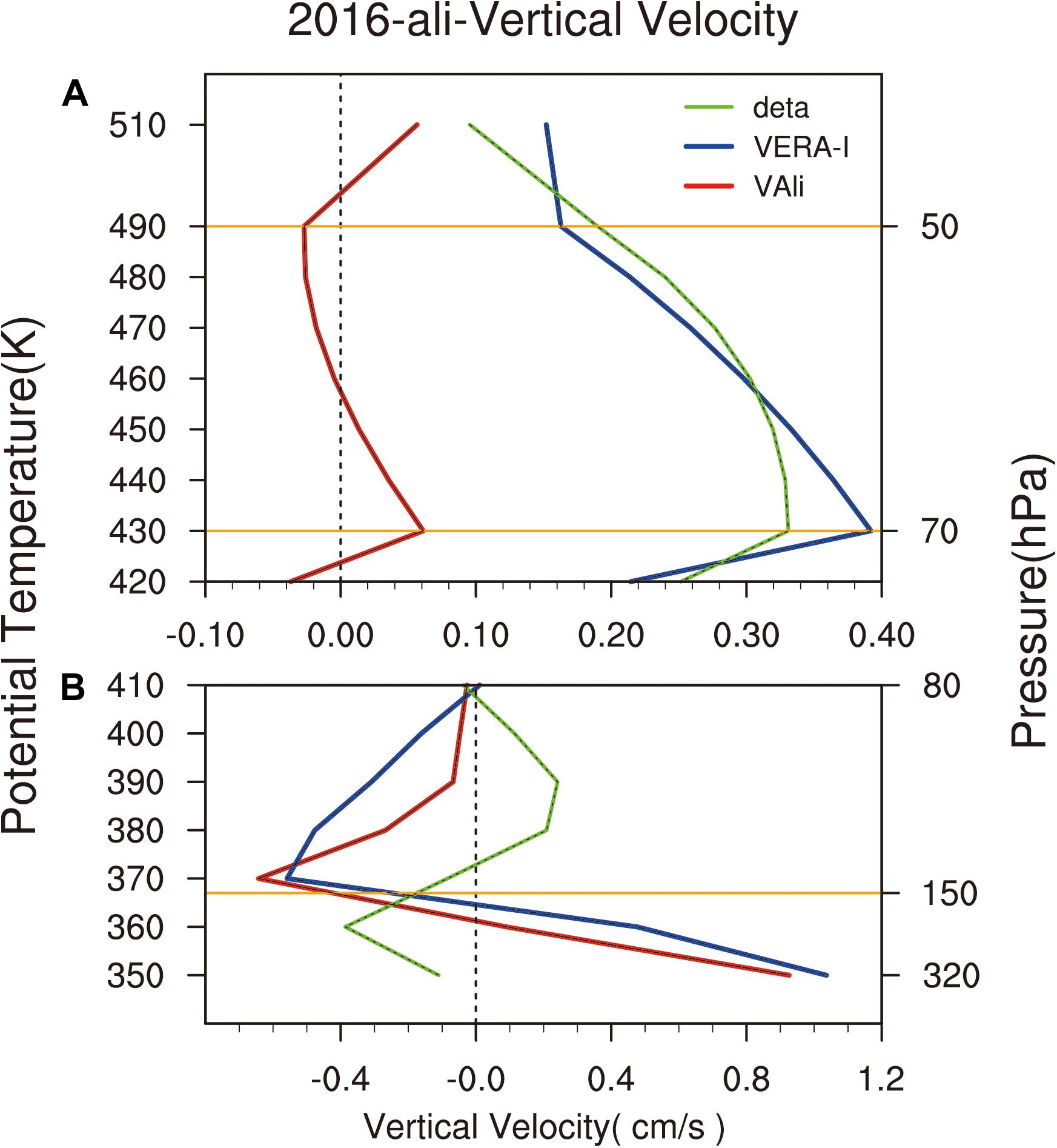
Figure 1. Vertical velocity profile at Ali station. The red line is V_Ali, the blue line is V_ERA–I, and the green line is the difference between the two. The three yellow lines represent levels of 50, 70, and 150 hPa. (A) and (B) had the different range of abscissa.

To avoid the influence of a single station, we compared V_AIRS with V_ERA–I in different layers (Figure 2). We chose the regional average over (32.5±2°N, 80.5±2°E) around Ali station to represent the single-point data. Figure 2 clearly shows that there are significant differences between day and night.

FIGURE 2

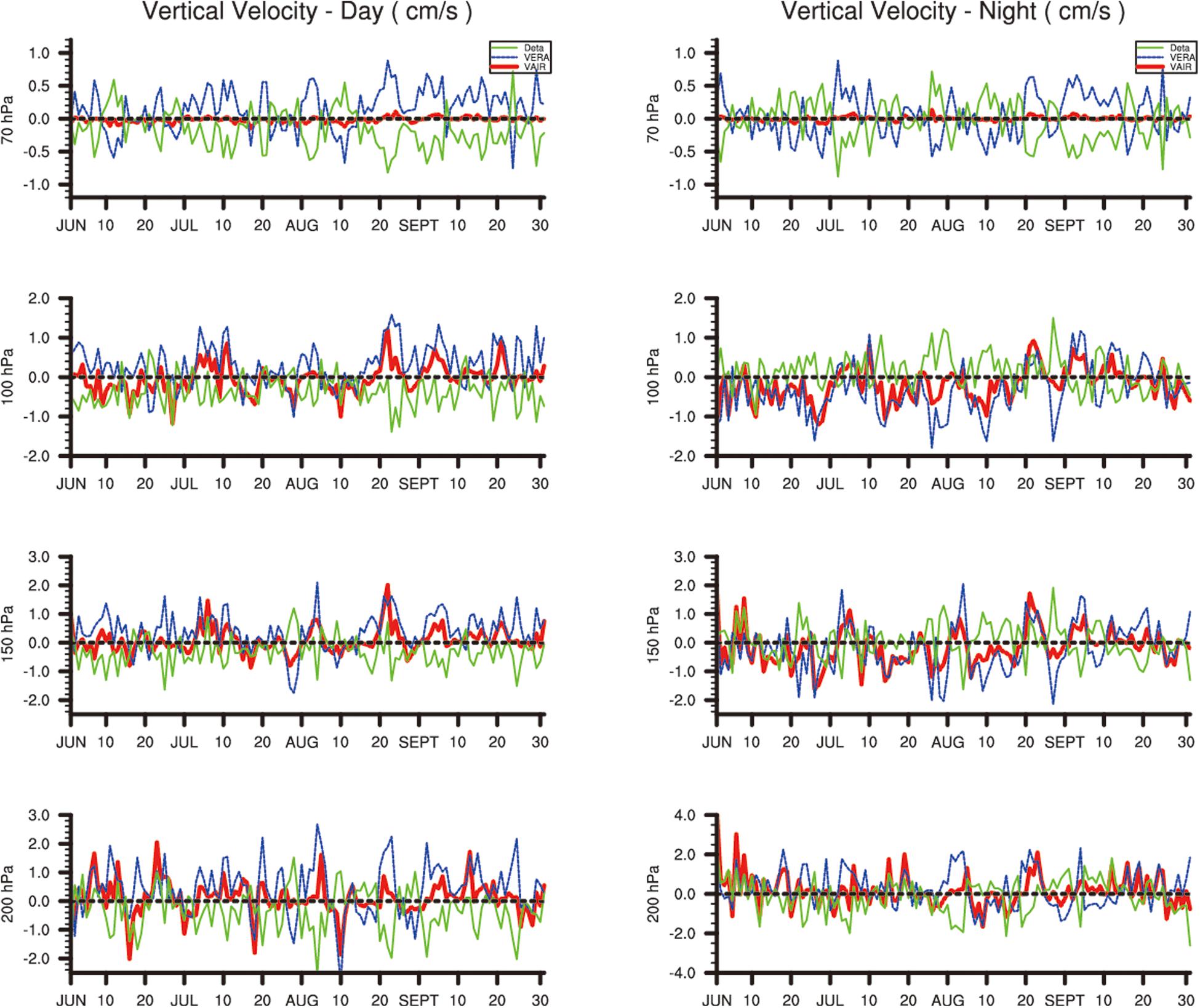
Figure 2. Time series of daily vertical velocity at different pressure layers in JJAS (June–September) 2012. The red and blue lines indicate V_AIRS and V_ERA–I, respectively, and the green lines represent the difference between the two values. The daytime and nighttime vertical velocity are shown in the left- and right-hand panels, respectively.

In the daytime, V_ERA–I (blue) describes a more pronounced upward movement in the region around Ali station that decreases with height. By contrast, V_AIRS only shows a clear ascending motion in the lower layers (200 and 150 hPa) and the values are much lower than V_ERA–I. V_AIRS approaches zero at 70 hPa.

At night, V_ERA–I shows an alternation from ascending to descending motion at 200 hPa and is dominated by descending motion in the range 150–100 hPa. V_ERA–I shows a remarkable upward motion in the higher layers around 70 hPa most of the time. V_AIRS shows the same variation as V_ERA–I, but with smaller values. This is because the radiation heating rate of the atmosphere in the UTLS in the daytime is mainly caused by shortwave solar radiation, which has a strong positive heating effect, leading to upward motion. Most of the heating at night is caused by longwave radiation from the ground, so the heating rate is negative, representing descending motion. The nighttime characteristic represented by V_AIRS is consistent with the results of V_Ali.

We examined the mean and standard deviation of V_AIRS and V_ERA–I in JJAS to conduct a more intuitive quantitative analysis and comparison (Figure 3). For the vertical velocity in 2012, V_AIRS and V_ERA–I are mostly positive in all the layers in the daytime (Figure 3A) and V_AIRS shows a much weaker updraft than V_ERA–I. V_AIRS reverses from positive to negative between 150 and 100 hPa, leading to wind convergence with a lower standard deviation; but this is not seen for V_ERA–I. The consistency of the distribution of V_AIRS and V_ERA–I increases during the night-time (Figure 3C), especially in the upper stratosphere. The reversal of winds appears near 150 and 80 hPa, consistent with V_Ali (Figure 1). The standard deviations also show that the dispersion of both V_AIRS and V_ERA–I gradually decreases with height in the daytime.

FIGURE 3

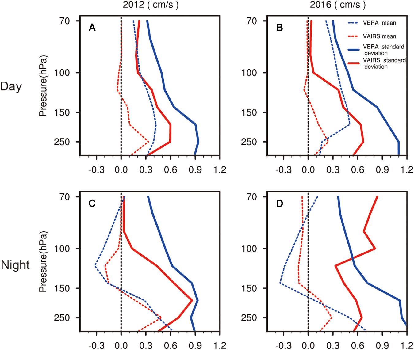
Figure 3. Mean (dashed lines) and standard deviation (solid lines) of V_AIRS and V_ERA–I in JJAS (units: cm s^–1) in 2012 (A,C) and 2016 (B,D). The blue lines are V_ERA–I and the red are V_AIRS. The upper panels are daytime and the bottom panels nighttime.

The overall distribution of the mean and standard deviation in 2016 were similar to those in 2012, but the differences between two vertical velocities were more significant than in 2012, especially in the lower stratosphere. The results in 2016 had a greater deviation, especially for V_AIRS at night.

We substituted V_AIRS and V_ERA–I into Eq. 13 and obtained the range (b - se, b + se) to investigate the mean bias and standard error of the vertical velocity (Figure 4). According to the daytime results for 2012 (Figure 4A) and 2016 (Figure 4B), the mean bias is concentrated near zero below 250 hPa, but is almost positive above 250 hPa. This shows that V_ERA–I differs slightly from V_AIRS in the lower layers, but that the difference is more pronounced at higher levels in the daytime. Above 250 hPa, the range (b - se, b + se) with the error bars does not contain 0. These results show that, in the daytime, the deviations all have more statistical significance above 250 hPa. In other words, V_ERA–I is generally higher than V_AIRS above 250 hPa.

FIGURE 4

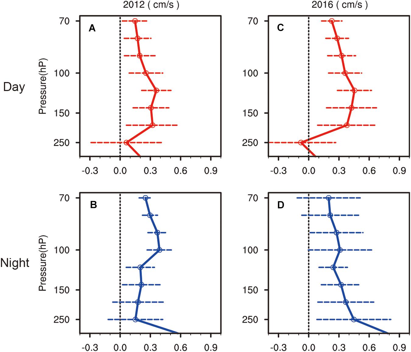
Figure 4. Average deviation (solid lines) and standard error (dashed lines) between V_AIRS and V_ERA–I for 2012 (A,B) and 2016 (C,D). The upper panels are daytime and the bottom panels nighttime.

The results for nighttime are different. In 2012, the mean bias was positive at all layers, which means that V_AIRS was smaller than V_ERA–I. But combined with the values of error bars, the results were statistically significant above 180 hPa, but insignificant at lower levels. Therefore V_ERA–I is larger than V_AIRS in the lower stratosphere and the deviation between them in the upper troposphere has more uncertainty. The situation was the opposite in 2016 and was statistically significant at lower levels (250–110 hPa), but not at higher levels.

Regional Comparison Analysis

Using (32.5°N, 80.5°E) as the center point, V_MLS was expanded along 32.5°N and 80.5°E to obtain the longitudinal and latitudinal vertical profiles. Figure 5 shows the characteristics of V_MLS and V_ERA–I during the daytime in 2012. The latitudinal profiles in Figures 5A,B show that both V_MLS and V_ERA–I have clear ascending motion in most areas of the ASMA and convergence at 80 hPa near 91.25°E (the center of the Qinghai–Tibet Plateau). But V_MLS shows descending motion in the west of 91.25°E and below 100 hPa, which is not shown in V_ERA–I. In terms of the deviation in Figure 5C, V_MLS has a weaker latitudinal ascending motion than V_ERA–I, especially above 100 hPa, where the differences pass the significance test. According to the longitudinal section in Figures 5D,E, upward motion appears simultaneously in most areas of V_ERA–I and V_MLS. Below 150 hPa, the ascending motion for V_MLS (Figure 5D) is as strong as V_ERA–I (Figure 5E), but above 150 hPa, V_MLS is clearly weaker than V_ERA–I. These differences also have passed the significance test (Figure 5F). In contrast, V_MLS is negative north of 34.4°N and near 100 hPa, although the intensity is not as strong as for the ascending motion.

FIGURE 5

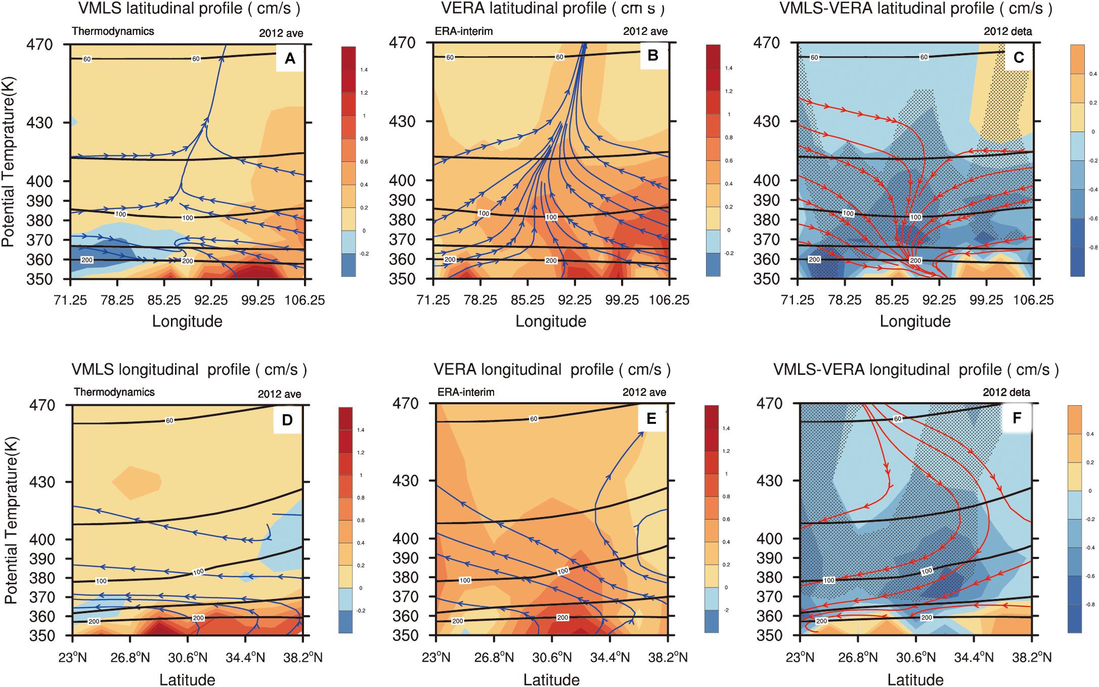
Figure 5. Daily mean V_MLS (A,D), V_ERA–I (B,E) and the deviation between them (C,F) for daytime in JJAS 2012. Panels (A–C) are the latitudinal profiles along 80.5°E and (D–F) are the longitudinal profiles along 32.5°N. The shading represents the vertical velocity field, the streamlines are the vertical and horizontal wind fields and the contour lines are the air layer. The dotted regions in panels (C,F) represent the area that passed the 95% significance test.

The nighttime conditions (Figure 6) are different from the daytime conditions (Figure 5). In the latitudinal profiles (Figures 6A,B), V_MLS shows strong descending motion below 150 hPa, whereas V_ERA–I shows significant ascending. Above 150 hPa, V_MLS is negative west of 91.25°E and positive to the east. Compared with the daytime, the area in which V_MLS is descending has expanded to lower and higher layers in the vertical direction. For V_ERA–I, descending motion is seen to the west of 91.25°E with a center of intensity near 100 hPa, but the vertical depth of the descending air is less than for V_MLS. The latitudinal profiles for V_MLS at nighttime and daytime both show descending motion in the west over the ASMA region. That probably indicates there is a difference in the descending branch of the Hadley Circulation in this region between V_MLS and V_ERA–I. The Hadley Circulation originally leads to a descending motion, but the stronger heating of the Qinghai–Tibet Plateau in the east and the weaker heating of the Iranian Plateau in the west (Zhang F. et al., 2017) finally introduced a more clearly upward motion over the Qinghai–Tibet Plateau. Thus, the atmosphere in the west descends while the atmosphere in the east ascends. V_MLS is more consistent with this explanation both day and night. Meanwhile, V_MLS and V_ERA–I both clearly show ascending movement in the east of the ASMA region. In the east of 99.25°E, between 100 and 70 hPa, V_MLS ascends significantly slowly than V_ERA–I, as illustrated in the test of deviation (Figure 6C).

FIGURE 6

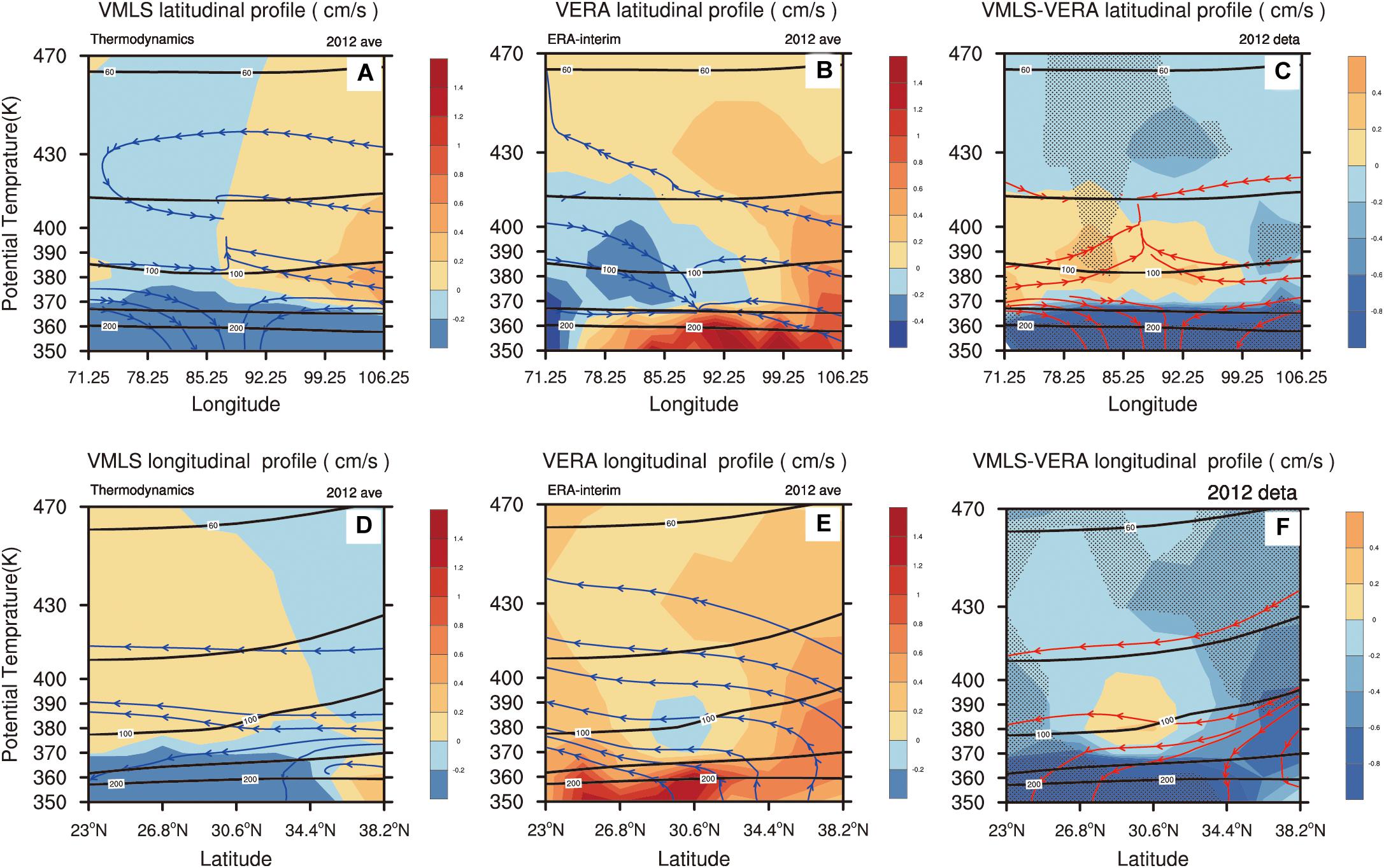
Figure 6. Daily mean V_MLS (A,D), V_ERA–I (B,E) and the deviation between them (C,F) for the nighttime in JJAS 2012. Panels (A–C) are the latitudinal profiles along 80.5°E and (D–F) are the longitudinal profiles along 32.5°N. The shading represents the vertical velocity field, the streamlines are the vertical and horizontal wind fields and the contour lines are the air layer. The dotted regions in panels (C,F) represent the area that passed the 95% significance test.

The longitudinal sections in Figures 6D,E show V_ERA–I ascending, but V_MLS descending in the northern part of the ASMA and in the lower layers below 150 hPa. With the local Hadley Circulation and the local Brewer-Dobson Circulation existing here, a downdraft occurs in this region. We suggest that V_MLS can describe the descending motion more clearly. The ascending movement of V_MLS is significantly weaker than V_ERA–I in the same region.

Figure 6 shows that V_MLS is mainly subsiding in the northwest and reaches the upper troposphere, whereas V_ERA–I is mainly subsiding in the lower layers in the west with a stronger intensity center. The descending motion of V_MLS below 150 hPa shows that there is a vertical divergence at 150 hPa in the west and north of the ASMA region. This result is consistent with that of V_Ali and V_AIRS at night.

Figure 7 shows the overall daily mean vertical velocity of JJAS in 2012. The distributions of both V_MLS and V_ERA–I are more consistent with the characteristics in daytime (Figure 5), indicating that the vertical motion in the ASMA region depends mainly on the vertical velocity in the daytime. The ascending movement of V_MLS is weaker than that of V_ERA–I, but still reflects the subsiding circulation in the western and northern ASMA.

FIGURE 7

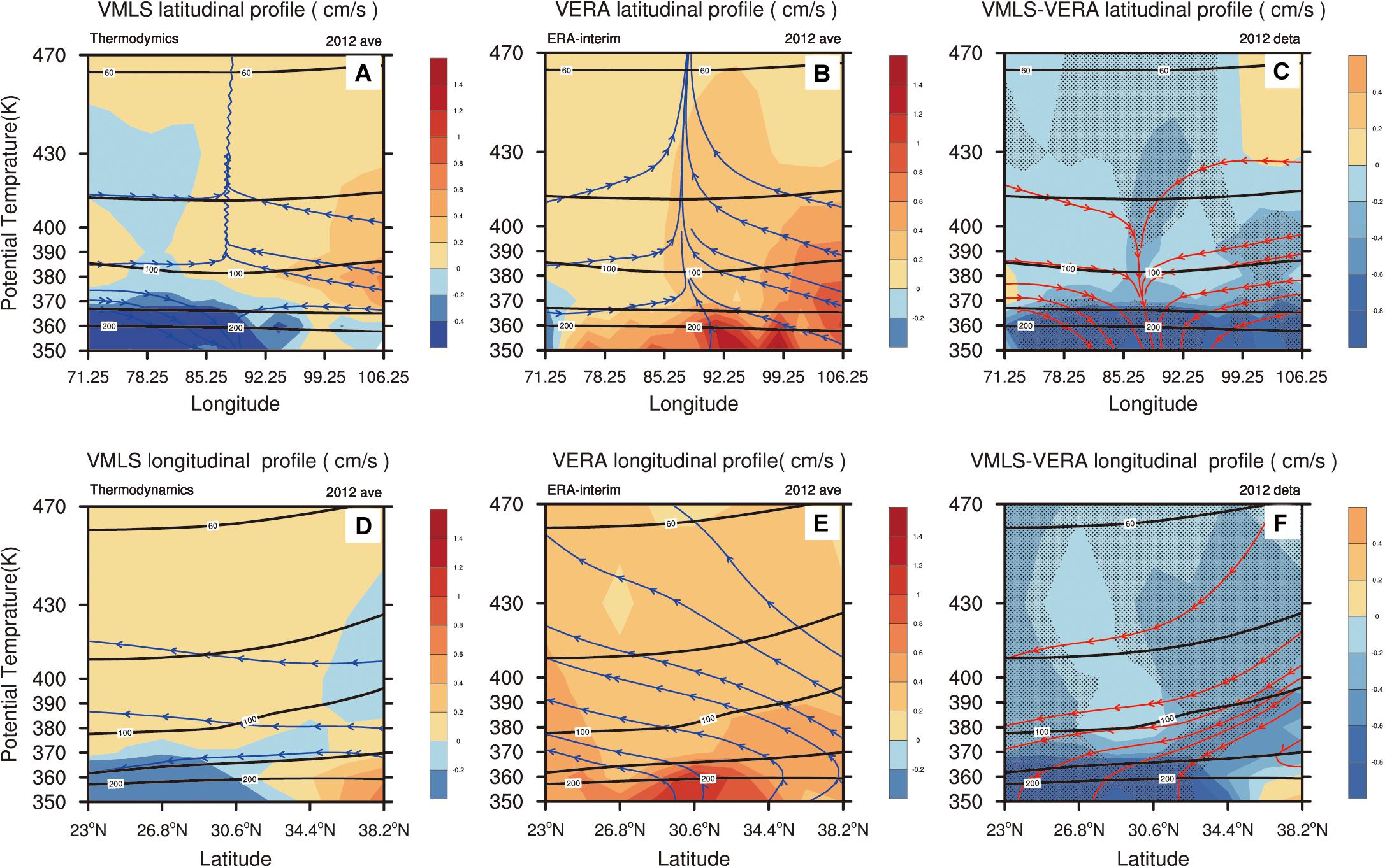
Figure 7. Daily mean V_MLS (A,D), V_ERA–I (B,E) and the deviation between them (C,F) in JJAS 2012. Panels (A–C) are the latitudinal profiles along 80.5°E and (D–F) are the longitudinal profiles along 32.5°N. The shading represents the vertical velocity field, the streamlines are the vertical and horizontal wind fields and the contour lines are the air layer. The dotted regions in panels (C,F) represent the area that passed the 95% significance test.

Discussion and Conclusion

Conclusion

The thermodynamic method has theoretical advantages over the kinematic method for calculating the vertical velocity over the ASMA region. We established a method based on the thermodynamic equation and introduced heating rate data obtained from in situ observations and revised satellite data from MLS/AIRS to determine the vertical velocity in JJAS 2012 and 2106. By comparing V_AIRS, V_Ali, and V_MLS with V_ERA–I, we found that V_Ali and V_ERA–I present similar behavior in upper troposphere, with a reversal of the wind direction near 150 and 80 hPa during the night in JJAS 2012. A comparison of V_AIRS and V_ERA–I showed that V_AIRS behaved differently from V_ERA–I at daytime. V_AIRS ascended weakly below 150 hPa and reversed to descending then reaches zero at 100 hPa, while V_ERA–I was clearly shown ascending in all layers. At nighttime, V_AIRS has similar behaviors of V_ERA–I with a weaker vertical motion intensity, which are also consistent with V_Ali. The differences between them have statistical significance with the degree of credibility in one standard error. We consider that V_AIRS is more in line with V_ERA–I in 2012 and better describes the vertical motion in the ASMA region.

The vertical profiles both day and night of V_MLS along (32.5°N, 80.5°E) illustrated that upward motions are in the east and south, and descending motions are in the west and north over the ASMA region, while V_ERA–I only showed descending motions in the west and north at the nighttime. The local flow of the Hadley Circulation and the Brewer-Dobson Circulation in this region may show a downdraft directly in the north. Besides, as a result of the weaker heating of the Iranian Plateau in the west than the Qinghai–Tibet Plateau in the east, the ascending motion over the Iranian Plateau is weaker than that over the Qinghai–Tibet Plateau (Zhang F. et al., 2017). Therefore, the vertical motions over the Iranian Plateau mainly present descending. We suggest that V_MLS can describe the vertical motions over the ASMA more accurately—that is, descending in the west and north and ascending in the east and south. The two vertical velocity profiles were similar in the ASMA region during the night-time. Based on the daily mean vertical velocity, we found that the vertical motion over the ASMA region mainly depends on the vertical velocity in the daytime.

Discussion

The thermodynamic vertical velocity we calculated is slightly weaker than the reanalysis data in some areas over the ASMA, which is inconsistent with the expectation that the velocity obtained by the kinematics method is insufficient. The probable reasons for this deviation are as follows. (1) The radiative heating rate used in this paper resulted in an inaccurate diabatic calculation. (2) For consistency, the variables u, v, T, and $\stackrel{.}{Q}$ were interpolated vertically to fixed isentropic (θ) levels. However, a variable in adjacent grids has different staggered changes in the vertical direction. After interpolation, the original vertical distribution characteristics would be eliminated, thereby introducing a deviation (Rex et al., 2008). (3) The deviations in the ERA-I dataset cannot be neglected and new reanalysis data should be analyzed in the future (Gao et al., 2014; Gianpaolo et al., 2015).

Data Availability Statement

The datasets generated for this study are available on request to the corresponding author.

Author Contributions

DG initiated and coordinated the work. DG and PS provided the calculation and analysis of vertical velocities. DG, PS, and MW wrote the manuscript. CS, YL, and MW gave valuable suggestions for revisions. CS and CZ revised the MLS and AIRS satellite data. WL calculated the heating rates.

Funding

This study was jointly supported by The National Key Research and Development Program of China (2018YFC1505602) and The National Science Foundation of China (91537213, 91837311, 41675039, and 41875048).

Conflict of Interest

The authors declare that the research was conducted in the absence of any commercial or financial relationships that could be construed as a potential conflict of interest.

Acknowledgments

We thank Professor Xiangdong Zheng from the Chinese Academy of Meteorological Sciences for providing the ozonesonde profiles and Professor Feng Zhang from Fudan University for providing the CanAM4.3_RAD model.

Footnotes

1. ^ https://apps.ecmwf.int/datasets/

References

Antokhin, P. N., and Belan, B. D. (2013). Control of the dynamics of tropospheric ozone through the stratosphere. J. Atmos. Ocean. Opt. 26, 207–213. doi: 10.1134/S1024856013030032

CrossRef Full Text | Google Scholar

Aschmann, J., Sinnhuber, B.-M., and Atlas, E. L. (2009). Modeling the transport of very short-livedsubstances into the tropical upper troposphere and lower stratosphere. Atmosp. Chem. Phys. 3, 9237–9247.

Google Scholar

Bergman, J. W., Fierli, F., Jensen, E. J., Honomichl, S., and Pan, L. L. (2013). Boundary layer sources for Asian anticyclone: regional contributions to a vertical conduit. J. Geophys. Res. 118, 2560–2575. doi: 10.1002/jgrd.50142

CrossRef Full Text | Google Scholar

Bergman, J. W., Jensen, E. J., and Pfister, L. (2012). Seasonal differences of vertical-transport efficiency in the tropical tropopause layer: on the interplay between tropical deep cobvection, large-scale vertical ascent, and horizontal circulations. J. Geophys. Res. 117:D05302. doi: 10.1029/2011JD016992

CrossRef Full Text | Google Scholar

Bian, J. C. (2009). Recent advances in the study of atmospheric vertical structures in upper troposphere and lower stratosphere. Adv. Earth Sci. 16(Suppl. 1), 116–122.

Google Scholar

Bian, J. C., Fan, Q. J., and Yan, R. C. (2013). Summertime stratosphere-tropospherestratosphere–troposphere exchange over the tibetan plateau and its climatic impact. Adv. Meteor. Sci. Technol. 2, 22–28.

Google Scholar

Bian, J. C., Li, D., Bai, Z. X., Li, Q., Lyu, D., and Zhou, X. (2020). Transport of Asian surface pollutants to the global stratosphere from the Tibetan Plateau region during the Asian summer monsoon. Natl. Sci. Rev. 5:nwaa005.

Google Scholar

Bian, J. C., Yan, R. C., and Chen, H. B. (2011a). Tropospheric pollutant transport to the stratosphere by Asian summer monsoon. Chin. J. Atmos. Sci. 35, 897–902.

Google Scholar

Bian, J. C., Yan, R. C., Chen, H. B., Lu, D., and Massie, S. T. (2011b). Formation of the summertime ozone valley over the Tibetan Plateau: the Asian summer monsoon and air column variations. Adv. Atmos. Sci. 28, 1318– 1325.

Google Scholar

Butchart, N., and Scaife, A. A. (2001). Removal of chlorofluorocarbons by increased mass exchange between stratosphere and troposphere in a changing climate [climate [J]. Nature 2001, 799–802.

Google Scholar

Chen, B., Xu, X. D., and Bian, J. C. (2010). Sources, path ways and time scales for the troposphere to stratosphere transport over Asian m on snoon regions in boreal summer. J. Chinese J. Atmos. Sci. 34, 495–505.

Google Scholar

Chen, D., Zhou, T. J., Ma, L. Y., Shi, C. H., Guo, D., and Chen, L. (2019). Statistical analysis of the spatiotemporal distribution of ozone induced by cut-off lows in the upper troposphere and lower stratosphere over northeast Asia. Atmosphere 10:696. doi: 10.3390/atmos10110696

CrossRef Full Text | Google Scholar

Chipperfield, M. P. (2006). New version of the TOMCAT/SLIMCAT offline chemical transport model: intercomparison of stratospheric tracer experiments. Q. J. R. Meteorol. Soc. 132, 1179–1203. doi: 10.1256/qj.05.51

CrossRef Full Text | Google Scholar

Cong, C. H., Li, W. L., and Zhou, X. J. (2001). Mass exchange between stratosphere and troposphere over the qinghai-tibet Qinghai–Tibet plateau and its vicinity. J. Chinese Sci. Bull. 46, 1914–1918.

Google Scholar

Considine, D. B., Logan, J. A., and Olsen, M. A. (2008). Evaluation of near-tropopause ozone distributions in the global modeling initiative combined stratosphere/troposphere model with ozonesonde data. Atmos. Chem. Phys. 8, 2365–2385.

Google Scholar

Davis, J., Collier, C., Davies, F., and Burton, R. (2007). Vertical velocity observed by Doppler lidar during cops – A case study with a convective rain event. Meteorol. Z. 22, 463–470.

Google Scholar

Deng, F., Jones, D. B. A., and Walker, T. W. (2015). Sensitivity analysis of the potential impact of discrepancies in stratosphere-tropospherestratosphere–troposphere exchange on inferred sources and sinks of CO2. Atmos. Chem. Phys. 15, 10813–10851.

Google Scholar

Dessler, A. E., and Sherwood, S. C. (2004). Effect of convection on the summertime extratropical lower stratosphere. J. Geophys. Res. 109:D23301.

Google Scholar

Dobbie, J. S., Li, J., and Chýlek, P. (1999). Two- and four-stream optical properties for water clouds and solar wavelengths. J. Geophys. Res. Atmos. 104, 2067–2080. doi: 10.1029/1998JD200039

CrossRef Full Text | Google Scholar

Elliot, S., and Rowland, F. S. (1987). Chlorofluorocarbons and stratospheric ozone [ozone. J. Chem. Educ. 64, 387–380.

Google Scholar

Eluszkiewicz, J., David, C., Richard, Z., Lee, E., Evan, F., Lucien, F., et al. (1996). Residual circulation in the stratosphere and lower mesosphere as diagnosed from Microwave Limb Sounder data. J. Atmos. Sci. 53, 217–240. doi: 10.1175/1520-04691996053<0217:RCITSA>2.0.CO;2

CrossRef Full Text | Google Scholar

Eluszkiewicz, J., Hemler, R. S., Mahlman, J. D., Bruhwiler, L., and Takacs, L. L. (2000). Sensitivity of age-of-air calculations to the choice of advection scheme. J. Atmos. Sci. 57, 3185–3201.

Google Scholar

Fan, Q. J., Bian, J. C., and Pan, L. L. (2017a). Atmospheric boundary layer sources for upper tropospheric air over the Asian summer monsoon region. Atmos. Oceanic Sci. Lett. 10, 358–363.

Google Scholar

Fan, Q. J., Bian, J. C., and Pan, L. L. (2017b). Stratospheric entry point for upper-tropospheric air within the Asian summer monsoon anticyclone. Sci. China Earth Sci. 60, 1685–1693.

Google Scholar

Fan, W. X., Wang, W. G., and Bian, J. C. (2008). The distribution of cross-tropopause mass flux over the Tibetan Plateau and its surrounding regions. Chin. J. Atmos. Sci. 32, 1309–1318.

Google Scholar

Fu, R., Hu, Y. L., Wright, J. S., Jiang, J. H., Dickinson, R. E., Chen, M., et al. (2006). Short circuit of water vapor and polluted air to the global stratosphere by convective transport over the Tibetan Plateau. Proc. Natl. Acad. Sci. U.S.A. 103, 5664–5669.

Google Scholar

Fueglistaler, S., Bonazzola, M., Haynes, P. H., and Peter, T. (2005). Stratospheric water vapor predicted from the Lagrangian temperature history of air entering the stratosphere in the tropics. J. Geophys. Res. Atmos. 110. doi: 10.1029/2004JD005516

CrossRef Full Text | Google Scholar

Gamelin, B., and Carvalho, L. (2017). Tropopause Ozone and Water Vapor Concentrations During the South American Monsoon System With AIRS Satellite Observations and MERRA-2 Data. Washington, DC: American Geophysical Union.

Google Scholar

Gao, L., Hao, L., and Chen, X. W. (2014). Evaluation of ERA-interim monthly temperature data over the Tibetan Plateau. J. Mountain Sci. 11, 1154– 1168.

Google Scholar

Gerber, E. P. (2015). The stratosphere and its coupling to the troposphere and beyond. J. Encycl. Appl. Comput. Mat. 2015:1676. doi: 10.1007/978-3-540-70529-1_573

CrossRef Full Text | Google Scholar

Gettelman, A., Kinnison, D. E., and Dunkerton, T. J. (2004). Impact of monsoon circulations on the upper troposphere and lower stratosphere. J. Geophys. Res. 109:D22101.

Google Scholar

Gianpaolo, B., Albergel, C., and Beljaars, A. (2015). ERA-Interim/Land: a global land surface reanalysis dataset. Hydrol. Earth Syst. Sci. 19, 389–407.

Google Scholar

Guo, D., Su, Y. C., Shi, C. H., and Xu, J. (2015). Double core of ozone valley over the Tibetan Plateau and its possible mechanisms. J. Atmos. Solar Terres. Phys. 13, 127–131.

Google Scholar

Guo, D., Su, Y. C., and Zhou, X. (2017). Evaluation of the trend uncertainty in summer ozone valley over the Tibetan Plateau in three reanalysis datasets. J. Meteorol. Res. 31, 431–437.

Google Scholar

Guo, D., Wang, P., Zhou, X., Liu, Y., and Li, W. (2012). Dynamic effects of the South Asian high on the ozone valley over the Tibetan Plateau. Acta Meteorol. Sin. 26, 216–228.

Google Scholar

He, Y., Sheng, Z., and He, M. (2020a). Spectral analysis of gravity waves from near space high-resolution balloon data in Northwest China. Atmosphere 11:133. doi: 10.3390/atmos11020133

CrossRef Full Text | Google Scholar

He, Y., Sheng, Z., and He, M. (2020b). The first observation of turbulence in northwestern china by a near-space high-resolution balloon sensor. Sensors 20:677. doi: 10.3390/s20030677

CrossRef Full Text | Google Scholar

Herman, R., Rosenlof, K. H., Ray, E. A., Bedka, K. M., Read, W. G., Chin, K., et al. (2017). Enhanced stratospheric water vapor over the summertime continental United States and the role of overshooting convection. Atmos. Chem. Phys. 17, 6113–6124.

Google Scholar

Holton, J. R. (1990). On the global exchange of mass between the stratosphere and troposphere. J. Atmos. Sci. 47, 331–344.

Google Scholar

Holton, J. R., Haynes, P. H., and McIntyre, M. E. (1995). Stratosphere troposphere exchange. Rev. Geophys. 33, 403–439.

Google Scholar

Hu, Y. Y., Ding, F., and Xia, Y. (2009). Long-term trend of stratospheric atmosphere under global changing conditions. J. Adv. Earth Sci. 024, 242–251.

Google Scholar

Huang, R., Wen, C., and Ke, W. (2018). Atmospheric dynamics in the stratosphere and its interaction with tropospheric processes: progress and problems. Chinese J. Atmos. Sci. 42, 463–487. doi: 10.3878/j.issn.1006-9895.1802.17250

CrossRef Full Text | Google Scholar

King, M. D., Menzel, W. P., Kaufman, Y. J., Tanre, D., Gao, B.-C., Platnick, S., et al. (2003). Cloud and aerosol properties, precipitable water, and profiles of temperature and humidity from MODIS. IEEE Trans. Geosci. Remote Sens. 41, 442–458. doi: 10.1109/TGRS.2002.808226

CrossRef Full Text | Google Scholar

Kishcha, P., Starobinets, B., and Alpert, P. (2007). Latitudinal variations of cloud and aerosol optical thickness trends based on MODIS satellite data. Geophys. Res. Lett. 34:L05810. doi: 10.1029/2006GL028796

CrossRef Full Text | Google Scholar

Kistler, R. E., Kalnay, E., Collins, W., and Saha, S. (2001). The NCEP-NCAR 50-year reanalysis: monthly means CD-ROM and documentation. Bull. Am. Meteorol. Soc. 82, 247–268.

Google Scholar

Krishnamurti, T. N., and Bounoua, L. (1996). An Introduction to Numerical Weather Prediction Techniques. Boca Raton, FL: CRC Press.

Google Scholar

Kuang, S., Newchurch, M. J., Burris, J., Wang, L., Knupp, K., and Huang, G. (2012). Stratosphere-to-troposphere transport revealed by ground-based lidar and ozonesonde at a midlatitude site. J. Geophys. Res. Atmos. 117:305. doi: 10.1029/2012JD017695

CrossRef Full Text | Google Scholar

Li, C. M., Hu, J. X., and Xu, J. H. (2005). Prediction on the influence of ozone depletion substance to the stratospheric ozone. China Environ. Sci. 25, 142–145.

Google Scholar

Li, J. N., and Barker, H. (2005). A radiation algorithm with correlated-k distribution. J. Atmos. Sci. 62, 286–309. doi: 10.1175/JAS-3396.1

CrossRef Full Text | Google Scholar

Li, J. N., Ma, X., Salzen, K.V., and Dobbie, S. (2008). Parameterization of sea salt optical properties anda related radiative forcing study. Atmos. Chem. Phys. 8, 4787–4798. doi: 10.5194/acp-8-4787-2008

CrossRef Full Text | Google Scholar

Li, Z. K., Qin, H., and Guo, D. (2017). Impact of ozone valley over the Tibetan Plateau on the South Asian high in CAM5. Adv. Meteorol. 2017:9383495. doi: 10.1155/2017/9383495

CrossRef Full Text | Google Scholar

Lindner, T. H., and Li, J. (2000). Parameterization of the optical properties for water clouds in the infrared. J. Climate 13, 1797–1805. doi: 10.1175/1520-0442(2000)013<1797:POTOPF>2.0.CO;2

CrossRef Full Text | Google Scholar

Liu, Y. (1998). Atmospheric ozone layer, ultraviolet radiation and human health. Adv. Geophys. 13, 103–110.

Google Scholar

Liu, Y. (2007). Trends of stratospheric ozone and aerosols over tibetan plateau. J. Acta 65, 938–945.

Google Scholar

Liu, Y., Li, W., and Zhou, X. (2003). Mechanism of formation of the ozone valley over the Tibetan Plateau in summer— transport and chemical process of ozone. Adv. Atmos. Sci. 20, 103–109.

Google Scholar

London, J., and Park, J. H. (2011). The interaction of ozone photochemistry and dynamics in the stratosphere. Three Dimens. Atmos. Model. 52, 1599– 1609.

Google Scholar

Lord, S. J., and Jacqueline, M. L. (1988). Vertical velocity structures in an axisymmetric, nonhydrostatic tropical cyclone model. J. Atmos. Sci. 45, 1453–1461.

Google Scholar

Lu, C. H., and Ding, Y. H. (2013). Advances in the study of stratospheric and tropospheric interactions. J. Prog. Meteorol. Technol. 2013, 6–21. doi: 10.3969/j.issn.2095-1973.2013.02.001

CrossRef Full Text | Google Scholar

Lv, D. R., Bian, J. C., and Chen, B. H. (2009). The frontier and importance of the study of stratospheric atmospheric processes. Adv. Earth Sci. 24, 221–228.

Google Scholar

Mahowald, N. M., Plumb, R. A., and Rasch, P. J. (2002). Stratospheric transport in a three-dimensional isentropic coordinate model. J. Geophys. Res. Atmos. 107, ACH3-1–ACH3-14.

Google Scholar

Monge-Sanz, B. M., Chipperfield, M. P., Simmons, A. J., and Uppala, S. M. (2007). Mean age of air and transport in a CTM: comparison of different ECMWF analyses. Geophys. Res. Lett. 34:L04801.

Google Scholar

Newman, P. (2014). “The Future of the Stratosphere and the Ozone Layer[C],” in Proceedings of the Agu Fall Meeting, (Washington, DC: AGU).

Google Scholar

Newman, P. A., Oman, L. D., and Douglass, A. R. (2009). What would have happened to the ozone layer if chlorofluorocarbons (CFCs) had not been regulated? Atmos. Chem. Phys. 9, 2113–2128.

Google Scholar

Oram, D. E., Ashfold, M. J., Laube, J. C., Gooch, L. J., Humphrey, S., Sturges, W. T., et al. (2017). A growing threat to the ozone layer from short-lived anthropogenic chlorocarbons. Atmos. Chem. Phys. Discuss. 2017, 1–20.

Google Scholar

Park, M., Randel, W. J., Gettelman, A., Massie, S. T., and Jiang, J. H. (2007). Transport above the Asian summer monsoon anticyclone inferred from Aura Microwave Limb Sounder tracers. J. Geophys. Res. Atmos. 112:309. doi: 10.1029/2006JD008294

CrossRef Full Text | Google Scholar

Pavlov, A. N., Stolyarchuk, S. Y., Shmirko, K. A., and Bukin, O. A. (2013). Lidar measurements of variability of the vertical ozone distribution caused by the stratosphere-troposphere exchange in the Far East Region. J. Atmos. Ocean. Opt. 26, 126–134. doi: 10.1134/S1024856013020115

CrossRef Full Text | Google Scholar

Ploeger, F., Konopka, P., Gunther, G., Groob, J. U., and Muller, R. (2010). Impact of the vertical velocity scheme on modeling transport in the tropical tropopause layer. J. Geophys. Res. Atmos. 115:301. doi: 10.1029/2009JD012023

CrossRef Full Text | Google Scholar

Platnick, S., King, M. D., Ackerman, S. A., Menzel, W. P., Baum, B. A., Riedi, J. C., et al. (2003). The modis cloud products: algorithms and examples from terra. IEEE Trans. Geosci. Remote Sens. 41, 459–473. doi: 10.1109/TGRS.2002.808301

CrossRef Full Text | Google Scholar

Randel, W. J., Garcia, R. R., and Wu, F. (2002). Time-dependent upwelling in the tropical lower stratosphere estimated from the zonal-mean momentum budget. J. Atmos. Sci. 59, 2141–2152.

Google Scholar

Randel, W. J., and Jensen, E. (2013). Physical processes in the tropical tropopause layer and their role in a changing climate. Nat. Geosci. 6, 169–176.

Google Scholar

Randel, W. J., Park, M., and Emmons, L. (2010). Asian monsoon transport of pollution to the stratosphere. Science 328, 611–613.

Google Scholar

Rex, M., Lehmann, R., and Wohltmann, I. (2008). Ascent rates, dehydration and vertical diffusion in the tropical tropopause region and lower stratosphere. Reunion Island Symposium 37:2605.

Google Scholar

Rodgers, C. D. (1990). Characterization and error analysis of profiles retrieved from remote sonde measurements. Geophys. Res. 95, 5587–5595.

Google Scholar

Rosenlof, K. (1995). Seasonal cycle of the residual mean meridional circulation in the stratosphere. J. Geophys. Res. Atmos. 100:5173. doi: 10.1029/94jd03122

CrossRef Full Text | Google Scholar

de Roode, S. R., Siebesma, A. P., Jonker, H. J. J., and de Voogd, Y. D. (2012). Parameterization of the vertical velocity equation for shallow cumulus clouds. J. Mon. Weather Rev. 140:2424. doi: 10.1175/MWR-D-11-00277.1

CrossRef Full Text | Google Scholar

Salzen, K. V., Scinocca, J. F., Mcfarlane, N. A., Li, J., Cole, J. N. S., Plummer, D., et al. (2013). The canadian fourth generation atmospheric global climate model (canam4). Part I: representation of physical processes. Atmos. Ocean 51, 104–125. doi: 10.1080/07055900.2012.755610

CrossRef Full Text | Google Scholar

Schauffler, S. M., Atlas, E. L., Blake, D. R., Flocke, F., Lueb, R. A., Lee-Taylor, J. M., et al. (1999). Distributions of brominated organic compounds in the troposphere and lower stratosphere. J. Geophys. Res. 104: 21513.

Google Scholar

Schoeberl, M. R., Douglass, A. R., Zhu, Z., and Pawson, S. (2003). Comparison of the lower stratospheric age spectra derived from a general circulation model and two data assimilation systems. J. Geophys. Res. 108:4113.

Google Scholar

Shepherd, T. (2002). Issues in stratosphere-tropospherestratosphere–troposphere coupling. J. Meteorol. Soc. Jpn. 80, 769–792.

Google Scholar

Sherman, L. (1953). Estimates of the vertical velocity based on the vorticity equation. J. Atmos. Sci. 10, 399–400.

Google Scholar

Shi, C. H., Huang, Y., and Guo, D. (2018). Comparison of trends and abrupt change of Asia High from 1979 to 2010 in Reanalysis and Radiosonde data. J. Atmos. Solar Terrest. Phys. 170, 48–54. doi: 10.1016/j.jastp.2018.02.005

CrossRef Full Text | Google Scholar

Shi, C. H., Zhang, C. X., and Guo, D. (2017). Comparison of electrochemical concentration cell ozonesonde and microwave limb sounder satellite remote sensing ozone profile for the center of the South Asian High. Remote Sens. 9:1012.

Google Scholar

Sofieva, V. F., Ialongo, I., Hakkarainen, J., Kyölä, E., Tamminen, J., Laine, M., et al. (2017). Improved GOMOS/Envisat ozone retrievals in the upper troposphere and the lower stratosphere. J. Atmos. Meas. Tech. 10, 231–246. doi: 10.5194/amt-10-231-2017

CrossRef Full Text | Google Scholar

Stohl, A., Bonasoni, P., Cristofanelli, P., Collins, W., Feichter, J., Frank, A., et al. (2003). Stratosphere-roposphere exchange: a review, and what we have learned from STACCATO. J. Geophys. Res. Atmos. 108, 469–474.

Google Scholar

Tang, Z., Guo, D., and Su, Y. C. (2019). Double cores of the Ozone Low in the vertical direction over the Asian continent in satellite data sets. Earth Planet. Phys. 3, 11–19.

Google Scholar

Tian, H. Y., Tian, W. S., Luo, J., Zhang, J., and Zhang, M. (2017). Climatology of cross-tropopause mass exchange over the Tibetan Plateau and its surroundings. Int. J. Climatol. 37, 3999–4014.

Google Scholar

Tian, W. S., Martyn, C., and Huang, Q. (2008). Effects of the Tibetan Plateau on total column ozone distribution. Tellus B 60, 622–635.

Google Scholar

Tian, W. S., Zhang, M., and Shu, J. C. (2009). Application and development prospect of middle atmosphere model. J. Adv. Earth Sci. 024, 252–261.

Google Scholar

Uma, K. N., and Rao, T. N. (2009). Characteristics of vertical velocity cores in different convective systems observed over Gadanki, India. Am. Meterol. Soc. 2009, 954–975.

Google Scholar

Vaughan, G., Price, J. D., and Howells, A. (1994). Transport into the troposphere in a tropopause fold. Q. J. R. Meteorol. Soc. 120, 1085–1103.

Google Scholar

Vernier, J. P., Pommereau, J. P., Garnier, A., Pelon, J., Larsen, N., Nielsen, J., et al. (2009). Tropical stratospheric aerosol layer from CALIPSO lidar observations. J. Geophys. Res. Atmos. 114:D00H10. doi: 10.1029/2009JD011946

CrossRef Full Text | Google Scholar

Von Clarmann, T. (2006). Validation of remotely sensed profiles of atmospheric state variables: strategies and terminology. Atmos. Chem. Phys. 6, 4311–4320.

Google Scholar

Wang, H., Wang, W., Ding, A., and Huang, X. (2019). Impacts of stratosphere-troposphere-transport on summertime surface ozone over Eastern China. J. Sci. Bull. 65, 253–334. doi: 10.1016/j.scib.2019.11.017

CrossRef Full Text | Google Scholar

Wang, Y., Wang, H., and Wang, W. A. (2020). Stratospheric intrusion-influenced ozone pollution episode associated with an intense horizontal-trough event. Atmosphere 11:164.

Google Scholar

Xie, F., Li, J., Tian, W., Feng, J., and Huo, Y. (2012). The Signals of El Niño Modoki in the tropical tropopause layer and stratosphere. Atmos. Chem. Phys. 12, 5259–5273.

Google Scholar

Xie, F., Li, J., Tian, W., Fu, Q., Jin, F.-F., Hu, Y., et al. (2016). A connection from Arctic stratospheric ozone to El Niño-Southern oscillation. Environ. Res. Lett. 11:124026.

Google Scholar

Yan, X., Zheng, X., Zhou, X., Vomel, H., Song, J. Y., Li, W., et al. (2015). Validation of Aura Microwave Limb Sounder water vapor and ozone profiles over the Tibetan Plateau and its adjacent region during boreal summer. Sci. China Earth Sci. 58, 589–603.

Google Scholar

Yan, X. L., Konopka, P., and Ploeger, F. (2019). The efficiency of transport into the stratosphere via the Asian and North American summer monsoon circulations. Atmos. Chem. Phys. 19, 15629–15649.

Google Scholar

Yang, J., Shen, Z., and Lu, D. (2004). Simulation of stratosphere–troposphere exchange effecting on the distribution of ozone over eastern Asia. Chin. J. Atmos. Sci. 28, 579–588.

Google Scholar

Yu, P., Rosenlof, K. H., and Liu, S. (2017). Efficient transport of tropospheric aerosol into the stratosphere via the Asian summer monsoon anticyclone. Proc. Natl. Acad. Sci. U.S.A. 2017, 6972–6977.

Google Scholar

Yu, Z. X., Guo, D., and Li, L. P. (2020). The characteristics and mechanism of Rossby-wave energy vertical propagation crosssing tropopause in South Asia High region. Chinese Grophys. 63, 73–85. doi: 10.6038/cjg2020L0626

CrossRef Full Text | Google Scholar

Zhan, R. F., and Li, J. P. (2012). Relationship of interannual variations of the stratosphere –troposphere exchange of water vapor with the Asian summer monsoon. Chinese J. Geophys. 55, 3181–3193. doi: 10.6038/j.issn.0001-5733.2012.10.001

CrossRef Full Text | Google Scholar

Zhang, F., Kun, W., and Li, J. N. (2018). Radiative transfer in the region with solar and infrared spectra overlap. J. Quant. Spectrosc. Radiat. Trans. 219, 366–378.

Google Scholar

Zhang, F., and Li, J. (2013). Doubling-adding method for delta-four-stream spherical harmonic expansion approximation in radiative transfer parameterization. J. Atmos. Sci. 70, 3084–3101.

Google Scholar

Zhang, F., Shen, Z., and Li, J. (2013). Analytical delta-four-stream doubling-adding method for radiative transfer parameterizations. J. Atmos. Sci. 70, 794–808.

Google Scholar

Zhang, F., Wu, K., Li, J., Yang, Q., Zhao, J.-Q., and Li, J. (2016). Analytical infrared delta-four-stream adding method from invariance principle. J. Atmos. Sci. 73, 4171–4188.

Google Scholar

Zhang, F., Wu, K., Liu, P., Jing, X. W., and Li, J. (2017). Accounting for Gaussian quadrature in four-stream radiative transfer algorithms. J. Quant. Spectrosc. Radiat. Trans. 192, 1–13.

Google Scholar

Zhang, H. X., Li, W. J., and Li, W. P. (2017). Spatial and temporal distribution characteristics of surface heat fluxes over both Tibetan Plateau and Iranian Plateau in boreal spring and summer and their relationships. J. Acta Meteorol. Sin. 75, 260–274.

Google Scholar

Zhang, H., Jing, X., and Li, J. (2014). Application and evaluation of a new radiation code under McICA scheme in BCC_AGCM2.0.1. Geosci. Model Dev. 7, 737–754.

Google Scholar

Zhang, H., Wang, Z., and Zhang, F. (2015). Impact of four-stream radiative transfer algorithm on aerosol direct radiative effect and forcing. Int. J. Climatol. 35, 4318–4328.

Google Scholar

Zhang, J., Tian, W., and Chipperfield, M. P. (2015). Persistent shift of the Arctic polar vortex towards the Eurasian continent in recent decades. Nat. Clim. Change 6:1094.

Google Scholar

Zhang, J., Tian, W., Xie, F., Chipperfield, M. P., Feng, W., Son, S.-W., et al. (2018). Stratospheric ozone loss over the Eurasian continent induced by the polar vortex shift. Nat. Commun. 9: 206.

Google Scholar

Zhang, J., Tian, W., Xie, F., Tian, H., Luo, J., Zhang, J., et al. (2014). Climate warming and decreasing total column ozone over the Tibetan Plateau during winter and spring. Tellus B 66:23415.

Google Scholar

Zheng, X. D., Tang, J., and Li, W. L. (1998). Observational study on total ozone amount and its vertical profile over Lhasa in the summer of 1998. J. Appl. Meteor. Sci. 11, 173–179.

Google Scholar

Zhou, X. G., Wang, X. M., and Tao, Z. Y. (2014). Review and Discussion of Isentropic Thinking and Isentropic Potential Vorticity Thinking. Meteorological 40, 521–529.

Google Scholar

Zhou, X. J., and Luo, C. (1994). Ozone valley over Tibetan plateau. J. Meteor. Res. 8, 505–506.

Google Scholar

Zhou, X. J., Luo, C., and Li, W. L. (1995a). The change of total ozone in China and the low value center of qinghai-tibet Qinghai–Tibet plateau. J. Chinese Sci. Bull. 40:1396.

Google Scholar

Zhou, X. J., Luo, C., and Li, W. L. (1995b). The column ozone variation in China and the low value ozone center over Tibetan Plateau. Chin. Sci. Bull. 40, 1396–1398.

Google Scholar

Zou, H., and Gao, Y. Q. (1997). Vertical ozone profile over Tibet using SAGE I and II data. Adv. Atmos. Sci. 14, 505–512.

Google Scholar

Appendix A

Beijing Climate Center Radiation Transfer Model

A radiation model in Canadian Atmospheric Global Climate Model called CanAM4.3_RAD (Salzen et al., 2013) is used in this study. In this model, the correlated-k distribution (CKD) method of Li and Barker (2005) is used for gaseous transmission, including most of the greenhouse gases H₂O, O₃, CH₄, CO₂, N₂O, CO, O₂, CFC and so on. To improve the accuracy of the calculation in the ASMA region, the H₂O and O₃ were introduced from the in situ observations at Ali station and the revised satellite sounding data of the MLS and AIRS (Shi et al., 2017). The cloud properties (e.g., cloud top pressure, cloud effective radius, cloud water path, cloud fraction) were provided by Level 3 Moderate Resolution Imaging Spectroradiometer (MODIS) gridded global monthly products (MOD08_M3) data (King et al., 2003; Platnick et al., 2003; Kishcha et al., 2007). The other gases components were constant set in model. Four solar bands are adopted in wavenumber ranges 14500–50000, 8400–14500, 4200–8400, 2500–4200 cm⁻¹ and nine infrared bands are adopted in wavenumber ranges 2200–2500, 1900–2200, 1400–1900, 1100–1400, 980–1100, 800–980, 540–800, 340–540, 0–340 cm⁻¹. Optical properties of aerosols and cloud particles vary relatively slowly with wavenumber so they are parameterized as appropriately weighted mean values over each of the wavenumber intervals with aerosols and cloud optical properties respectively (Dobbie et al., 1999; Lindner and Li, 2000; Li et al., 2008). To achieve the high accuracy of heating/cooling rates, we use the adding method of four-stream spherical harmonic expansion approximation (4SDA) for solar radiation (Zhang and Li, 2013) and the adding method of four-stream discrete ordinates (4DDA) for infrared radiation (Zhang et al., 2016; Zhang J. et al., 2018; Zhang H.X. et al., 2017).