Englacial Warming Indicates Deep Crevassing in Bowdoin Glacier, Greenland

All around the margins of the Greenland Ice Sheet, marine-terminating glaciers have recently thinned and accelerated. The reduced basal friction has yielded increased flow velocity, while the rate of longitudinal stretching has been limited by ice viscosity, which itself critically depends on temperature. However, ice temperature has rarely been measured on such fast-flowing and heavily crevassed glaciers. Here, we present a 3-year record of englacial temperatures obtained 2 (in 2014) to 1 km (in 2017) from the calving front of Bowdoin Glacier (Kangerluarsuup Sermia), a tidewater glacier in northwestern Greenland. Two boreholes separated by 165 (2014) to 197 m (2017) show significant temperature differences averaging 2.07°C on their entire depth. Englacial warming of up to 0.39°C a⁻¹, an order of magnitude above the theoretical rate of heat diffusion and viscous dissipation, indicates a deep and local heat source within the tidewater glacier. We interpret the heat source as latent heat from meltwater refreezing in crevasses reaching to, or near to, the bed of the glacier, whose localization may be controlled by preferential meltwater infiltration in topographic dips between ogives.

1. Introduction

In many parts of the world, glaciers have recently slowed down as they thinned (Heid and Kääb, 2012; Dehecq et al., 2019). Yet this behavior has not been not ubiquitous. Around the margins of the Greenland Ice Sheet, marine-terminating outlet glaciers have also thinned, but they have accelerated and retreated faster than any of its other parts (e.g., Krabill et al., 2000; Rignot and Kanagaratnam, 2006; Pritchard et al., 2009; Moon et al., 2012, 2015; Hill et al., 2017), significantly impacting the total mass loss of the ice sheet (e.g., Enderlin et al., 2014; Khan et al., 2015; McMillan et al., 2016).

These tidewater glaciers are partly submerged in sea water, so that, as the glaciers have thinned, the gravitational force acting on the ice have increasingly been counterbalanced by buoyancy forces from the ocean. Basal friction has been reduced and the glaciers have flown faster, thus thinning even more (Meier and Post, 1987). When the glaciers come close to floatation, basal drag is drastically reduced (Shapero et al., 2016). Longitudinal stress coupling then becomes apparent through the upstream propagation of tidal velocity variations (Walters, 1989; Walter et al., 2012; Sugiyama et al., 2014; Podolskiy et al., 2017; Seddik et al., 2019). In such conditions, the increased flow velocities and longitudinal stretching are largely controlled by the ice viscosity. However, ice viscosity depends critically on temperature. Between −15°C and the pressure-melting point, ice softness varies by as much as an order of magnitude (Cuffey and Paterson, 2010, p. 72). Numerical models show that such differences in ice viscosity influence the flow and shape of entire glaciers and ice sheets (e.g., Figures 2, 7 of Seguinot et al., 2016).

Previous measurements show that glacier ice temperatures can be below the pressure-melting point (cold ice), at the pressure-melting point (temperate ice), or both (polythermal glacier) (Ahlmann, 1935; Cuffey and Paterson, 2010, p. 399). Glacier temperatures are primarily controlled by air temperatures, geothermal heat flux, viscous dissipation, and internal heat advection and diffusion (de Q. Robin, 1955), but can also be affected by latent heat released by meltwater refreezing in crevasses (Phillips et al., 2010, 2013; Colgan et al., 2011; Lüthi et al., 2015).

Much of this knowledge comes from measurements conducted on mountain glaciers and the interior of ice sheets. Ice temperature measurements from tidewater glaciers are presently available near the calving front for Svalbard (Jania et al., 1996) but limited to upstream areas in Greenland (Iken et al., 1993; Lüthi et al., 2002; Lüthi et al., 2015; Doyle et al., 2018), as heavy crevassing has typically hindered accessibility and posed practical and technical challenges to instrumentation near the glacier front.

Here, we present a new, 3-year, continuous record of englacial temperature from Bowdoin Glacier (Kangerluarsuup Sermia), a tidewater outlet glacier of the northwestern Greenland Ice Sheet. Despite some data gaps, the record reveals new mechanisms controlling temperature variations in a tidewater glacier.

2. Methods

2.1. Bowdoin Glacier

Bowdoin Glacier (Kangerluarsuup Sermia) is a tidewater glacier located in northwestern Greenland. It is a medium-size outlet glacier of the Greenland Ice Sheet with a catchment of about 60 × 60 km, and drains into Bowdoin Fjord across a 3 km-wide calving front (Figures 1a, 2a). The glacier front is located ca. 30 km from the settlement of Qaanaaq (see Figure 1 of Sugiyama et al., 2015, for a map).

FIGURE 1

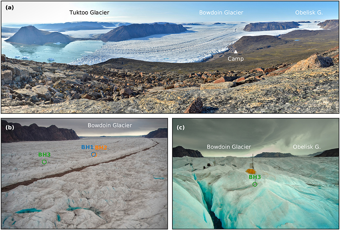
Figure 1. (a) Bowdoin Glacier panoramic view on 2015 July 17. The calving front is ca. 3 km wide and 50 m high. Note the steeper section of the glacier above the confluence of Obelisk Glacier. (b) Bowdoin Glacier lower drilling site and BH3 data loggers for thermistor strings and the basal piezometers on 2016 July 19. The data logger for the digital inclinometers was removed after cable damage related to the opening of the crevasse pictured. (c) Aerial view of the drilling sites on 2016 July 21. The location of BH1 and BH3 could be inferred from visible field installations.

FIGURE 2

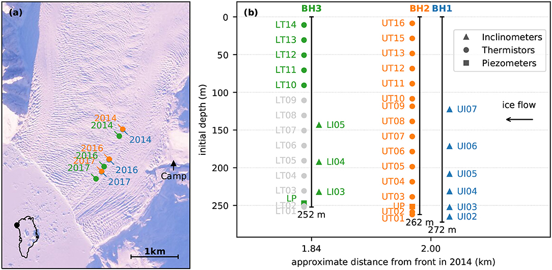
Figure 2. (a) Bowdoin borehole locations from drilling in July 2014 to dismantling in July 2017 and background satellite image from 2017 Mars 10, 17:41:29 UTC. Contains modified Copernicus Sentinel data, processed with Sentinelflow. (b) Initial ice thickness and sensor depths. Inclinometers and piezometers are also equipped with thermistors.

The glacier was chosen for fieldwork due to its accessibility, and the previously observed propagation of the mass loss of the Greenland Ice Sheet from the south to the northwest (Khan et al., 2010), although the more recent satellite gravimetry data shows that virtually all margins of the Greenland Ice Sheet are now loosing mass (Groh and Horwath, 2016). The surface of Bowdoin Glacier is heavily crevassed but parts of it are accessible on feet (Figures 1b,c). Crevasses are particularly few along a ca. 20 m-wide medial moraine (Figure 68 of Chamberlin, 1897), which can generally be walked down to the glacier front (Figures 1a,b).

Bowdoin Glacier was first visited by western explorers in the late-nineteenth century, who reported a “daily movement” of 0.85 m for July 1893 “at the fastest point” of the glacier (Chamberlin, 1894). Photographs indicate that Bowdoin Glacier was thicker at that time, but its frontal position was only a few kilometers downstream from the present calving front (Chamberlin, 1895, p. 668; Figures 64, 65 of Chamberlin, 1897; Figure 1 of Podolskiy et al., 2016) and has been relatively stable since then.

However, a two-fold increase of surface velocity in the early 2000s was followed by a rapid frontal retreat of Bowdoin Glacier by ca. 2 km between 2007 and 2013 (Figure 2 of Sugiyama et al., 2015), a behavior synchronous to that of other tidewater glaciers in the area (Sakakibara and Sugiyama, 2018). Since 2013, the ice front has appeared once again stable, yet the terminal tongue has continued to experience surface lowering at an alarming rate of ca. 4.1 m a⁻¹, which is primarily the expression of continued dynamic thinning (Tsutaki et al., 2016).

Bowdoin Glacier longitudinal strain and seismicity has varied in response to tides (Podolskiy et al., 2016, 2017) indicating a low basal drag and near plug-flow conditions (Seddik et al., 2019). Major icebergs have calved according to a recurring pattern in which fractures have propagated nearly parallel the to ice front (Jouvet et al., 2017). The emergence of subglacial meltwater has formed several submarine plumes of highly variable surface imprint (Jouvet et al., 2018) and entrained nutrients from the bottom to the surface of Bowdoin Fjord (Kanna et al., 2018).

2.2. Drilling Sites

During the field campaign in July 2014, three boreholes BH1 (272 m deep), BH2 (262 m), and BH3 (252 m) were drilled with hot water in the marine (glacier bed below sea level) part of Bowdoin Glacier using meltwater from the crevasses. After the successful drilling of BH1 and BH2, 7 m apart, at the first (upper) drilling site, 2 km from the calving front, it was planned that two other boreholes would be drilled upstream in the thicker part of the glacier. Due to unfavorable weather the hot water drilling equipment could not be transported upstream. Thus, a third and last hole was drilled 158 m downstream of the first borehole site to be equipped with all instruments left (Figures 1b, 2a).

Although the experiment was originally planned for 1 year, some of the instruments were let on the glacier for up to 3 years as more funding was obtained and additional field campaigns were planned for parallel experiments. From the drilling in July 2014 to the last data retrieval in July 2017, the boreholes were displaced by 997 (BH1) to 1191 m (BH3), their surface lowered from 89 (BH1, 2014) to 54 m above sea level (BH3, 2017) and the distance between the lower (BH3) and upper (BH1) drilling sites increased from 158 to 191 m (Figure 2a). New crevasses appeared on the glacier surface, some causing damage to the instruments (Figure 1c).

2.3. Instrumentation

The boreholes were equipped with three types of sensors: strings of simple, regularly-spaced thermistors arranged to span the entire depth of the glacier, two piezometers near the base of the glacier, and digital inclinometer units at different depths. Besides their primary sensors, the piezometers and digital inclinometers were equipped with additional thermistors, so that ice temperature could be measured at multiple depths in the glacier. This manuscript focuses on the temperature data. The tilt data are used to estimate strain heating.

At the first (upper) drilling site, one borehole (BH1) was equipped with seven digital inclinometers (Figure 2b, blue triangles) and the other (BH2) with one basal piezometer (Figure 2b, orange square) and two thermistor strings (Figure 2b, orange circles). At the second (lower) drilling site, the borehole (BH3) was equipped with five digital inclinometers (Figure 2b, green triangles), one basal piezometer (Figure 2b, green square) and two thermistor strings (Figure 2b, green and gray circles).

Due to the relocation of the second drilling site the thermistor strings were re-arranged to fit a smaller ice thickness. However, the deeper thermistor string depict temperatures incompatible with those recorded by digital inclinometers in the same hole. The depths of digital inclinometers were calibrated from independent pressure sensors and are thus more robust than those of sensors on the thermistor string. Thus, we think that sensors on the thermistor string were misplaced due to a manipulation error and mark their positions and data as erratic (ERR, Figure 2b, gray circles). The error most likely occurred when cables were re-arranged and taped together for the installation of all remaining instruments in a single (BH3) borehole instead of the two originally planned. This decision was made in light of the observed diminishing availability of surface meltwater for drilling in this part of the glacier.

The basal piezometers (Geokon 4500) were connected to Campbell CR10X data loggers via Campbell AVW1 vibrating wire interfaces. The thermistor strings (NTC Fenwal 135-103FAG-J01, Ryser, 2014) were connected to Campbell CR1000 data loggers via Campbell AM416 relay multiplexers. The piezometers and thermistor strings data loggers were each powered by a 12 V, 24 Ah lead battery, and mounted in polyester cases on tetrapods (Figure 1c). These batteries were recharged during the 2015 and 2016 field campaigns using a petrol generator at the camp. For the thermistor strings, in addition to automatic measurements, manual readings were performed in 2015, 2016, and 2017 using a hand-held ohmmeter.

The digital inclinometers units (DIBOSS, Ryser, 2014; Ryser et al., 2014a,b) are equipped with VTI Technologies SCA103T inclinometers and iST TSic 716 temperature sensors and were connected to CR1000 data loggers. Each data logger was set-up in a hard plastic case including three 12 V, 65 Ah lead batteries and a solar panel on the outside, and anchored to an aluminum pole drilled into the ice. In the case of digital inclinometers, the observed resistance from the thermistors were converted to temperature values in situ by the englacial digitizers, thus avoiding to record the resistance of the borehole cables and their potential variations due to cable deformation. The deployment and maintenance of the borehole installations was eased by the medial moraine (Figure 1b).

Finally, a dual frequency Global Positioning System (GPS) receiver was installed near the first borehole (BH1). A GPS antenna (JAVAD GrAnt-G3T) was mounted on an aluminum stake re-drilled every summer in the ice to accommodate melt. It was connected to a GPS receiver (GNSS Technology Inc. GEM-1) set-up in a hard plastic case and powered by an external ca 30 Ah lead battery and a solar panel. The same GPS instruments were installed near the camp site as a reference station for post-processing (Figure 2a, black triangle).

2.4. Experiment Duration

Of the total 44 sensors installed, 41 worked after the installation, 38 recorded data for 1 year, 35 were still functional after 2 years (of which 16 were not connected to a data logger any longer but were used for a manual temperature reading), and only two were left working after 3 years. Contact to sensors was progressively lost due to a battery issue (2014 July 28 and again 2015 July 26, one sensor) cable damage during the installation (2014 July 16 and 23, three sensors) cable damage at depth (2014 Oct. 25, 2017 Jan. 28, Feb. 03, and June 21, five sensors), and most importantly, cable damage at the surface (2015 Nov. 12 and unknown dates, 33 sensors, Table 1, Figure 1c).

TABLE 1

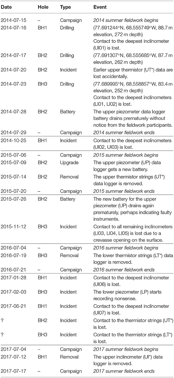
Table 1. Timeline of events including borehole drilling locations and initial depths, instrumental failures, and final removal (dates as YYYY-MM-DD).

2.5. Temperature Calibration

For the thermistor strings, the conversion from resistance to temperature is performed during post-processing following the Steinhart-Hart equation:

$\begin{array}{ll}\frac{1}{T}=a_0+a_{1}log(R)+a_{3}log{(R)}^3,& (1)\end{array}$

where R is the measured resistance, T the ice temperature, and a₀, a₁, and a₃ are coefficients calibrated individually for each sensor prior to fieldwork in the lab for temperatures of −15, −12, −9, −6, −3, and 0 °C (Table 2). The basal piezometers use temperature calibration coefficients published by the manufacturer (Table 2). The thermistors included in digital inclinometers were calibrated by the manufacturer and deliver direct temperature values with a published accuracy of 70 mK and resolution of 4 mK (Ryser, 2014, p. 44).

TABLE 2

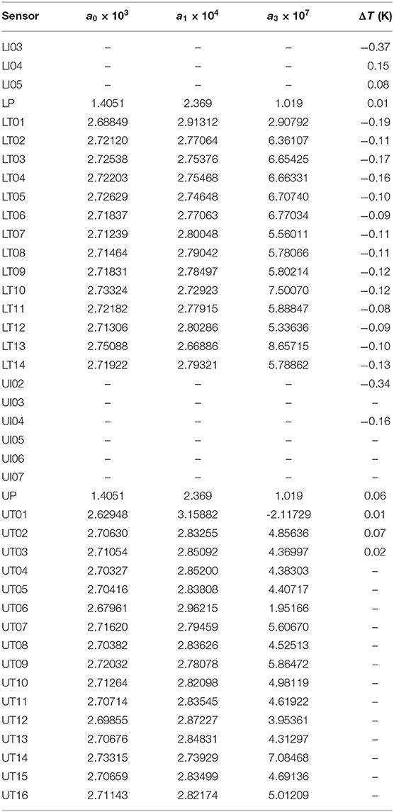
Table 2. Temperature calibration coefficients and melt offset corrections.

Despite the pre-field calibration, the temperatures observed in the meltwater-filled borehole immediately after drilling were not at the pressure-melting point but instead up to 0.16 °C colder. As we can not exclude that the initial calibration was affected by the transport of the instruments to Greenland, an in-situ recalibration is applied in post-processing by correcting for the initial temperature offset to the pressure melting-point, ΔT (Table 2). Unfortunately some of these initial temperature data were lost so that the recalibration was possible for some sensors only. The pressure-melting point was computed as

$\begin{array}{ll}{T}_m=-\beta \rho gz,& (2)\end{array}$

where β is the Clausius-Clapeyron constant, ρ is the ice density, g is the standard acceleration due to gravity, and z is the depth below the ice surface (parameter values given in Table 3). Because the Clausius-Clapeyron constant may be affected by impurities, we use a value determined in similar condition for another water-filled borehole in Greenland (Lüthi et al., 2002).

TABLE 3

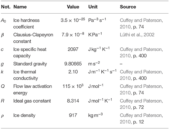
Table 3. Parameter values used to compute the theoretical englacial warming.

3. Results

3.1. Temperature Time Series

After the drillings, some sensors in BH2 record hourly air temperature variations as they are temporarily located above the borehole water level. However, most sensors are immersed and temperatures are measured at or near the pressure-melting point (Table 2). For most sensors temperatures then drop off the pressure-melting point and follow an S-curve before stabilizing at −0.25 to −6.04 °C (Figure 3; cf. Figure 3.6 of Ryser, 2014). This initial phase lasts for hours to months depending on the sensor and relating to the equilibrium temperature. While most records reach a thermal equilibrium within 3 months, sensors LT03 and LT02 recorded freezing after 11 and 15 months, reaching respective minimum temperatures of −0.35 and −0.25 °C (Figure 3).

FIGURE 3

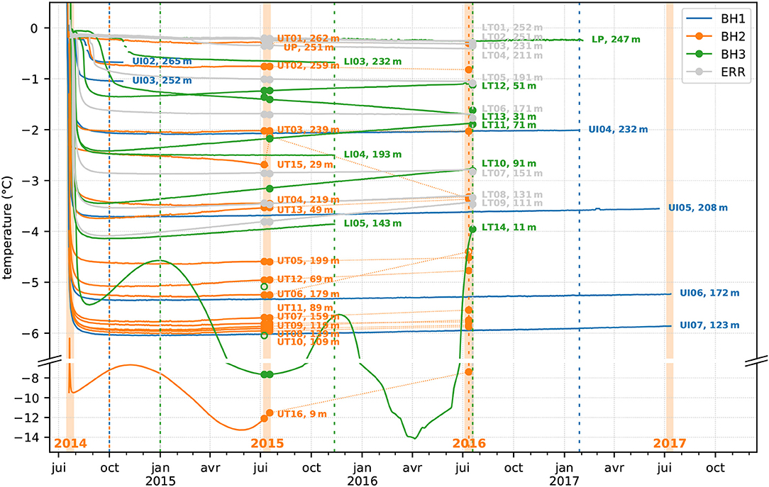
Figure 3. Ice temperature time series from the three boreholes (BH1, BH2, and BH3) including BH3 erratic data (ERR, see text) from the drilling in July 2014 to the last data retrieval in July 2017, and manual temperature readings (circles, with outliers marked as empty circles, and 2017 values off the graph). Field campaigns (verical orange spans) and the dates selected for temperature profiles (vertical dashed lines; Figure 4) are indicated.

The sensors nearest to the ice surface exhibit a seasonal temperature cycle, which is out-of-phase with the atmospheric temperature cycle (Figure 3, lowermost curves). The amplitude increases with time as the thermistor strings progressively melt-out toward the glacier surface, and may be affected by sunlight penetrating the ice. Temperature records for sensors installed deeper down in the ice do not show a seasonal cycle, but many exhibit a slow warming trend of 0.1 to 0.4°C a⁻¹ (Figure 3).

Manual temperature readings are generally compatible with the automatic records (Figure 3, filled circles), but some of these measurement are off by a few degrees, perhaps due to wet connectors (Figure 3, empty circles). Manual readings were also performed in 2017 but yielded values well-off the expected range, which is certainly due to surface cable damage visibly caused by opening crevasses (Figure 1b).

3.2. Temperature Profiles

After the refreezing of the entire boreholes, vertical profiles depict temperatures below the pressure-melting point except for the base of the glacier where temperatures reach the pressure-melting point (Figure 4a, Table 4). A thin layer of temperate ice possibly exists near the base but it is not revealed by the resolution of our measurements. The coldest temperatures of −6.03 (BH1), −5.98 (BH2) and −4.10 °C (BH3) are reached in the middle part of the ice column. Both profiles exhibit a subsurface layer with warmer temperatures up to −3.74 (BH2) and −1.35 °C (BH3), and a surface layer with seasonal temperature variations (Figure 4a).

FIGURE 4

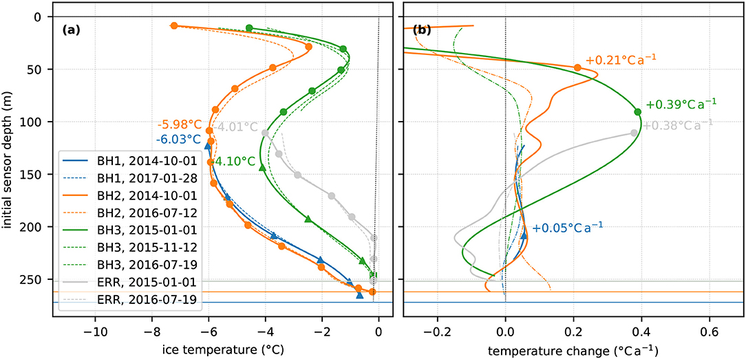
Figure 4. (a) Temperature profiles for selected dates (see Figure 3) ca. 2–5 months after the drilling (solid lines) and toward the end of the available record (dashed lines), for the three boreholes (BH1, BH2, and BH3) including BH3 erratic data (ERR, see text). The second profile from BH2 (orange dashed lines) corresponds to manual readings. Other values are daily means from the automated record. Borehole initial basal depths (thin horizontal lines) and minimum observed non-seasonal temperatures are indicated (dates as YYYY-MM-DD). (b) Observed rate of change between the two first profiles (solid lines) and theoretical change due to heat diffusion and viscous dissipation (dash-dotted lines) for the corresponding time period. The maximum observed warming is indicated. All curves were interpolated using cubic splines.

TABLE 4

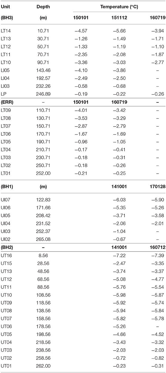
Table 4. Selected daily mean temperature values corresponding to profiles shown on Figure 4a (dates as YYMMDD).

The upper boreholes, BH1 and BH2, which are only separated by seven meters, show compatible temperature profiles with differences within 0.52°C (Figure 4a, blue and orange lines). For the lower borehole, the deepest thermistor string (ERR, Figure 4a, gray lines) depict temperatures incompatible with those recorded by digital inclinometers in the same hole (BH3, Figure 4a, green lines), whose depths were calibrated using independent pressure sensors.

Remarkably, the upper (BH1, BH2) and lower (BH3, ERR) drilling sites are located on the same flow line and separated by only 158 (2014) to 191 m (2017) but show temperature differences around 2°C prevailing over the entire glacier depth. BH1 and BH3 are separated by 158 (2014) to 191 m and show an average temperature difference of 1.81°C and a maximum of 2.11°C after interpolation over the lower part of the ice column where BH1 data are available (Figure 4a, blue and green lines). BH2 and BH3 are separated by 165 (2014) to 197 m (2017) and show an average temperature difference of 2.07 °C and a maximum of 2.86°C after interpolation (Figure 4a, orange and green lines).

All three temperature profiles show a general warming trend, except for their base (Figures 4a,b, solid lines). The warming trend of the upper drilling site (BH1, BH2) is within 0.1°C a⁻¹ except for the upper part where a maximum warming of 0.21°C a⁻¹ is observed (Figure 4, blue and orange lines). On the other hand, the lower (BH2, ERR) drilling site experiences significant englacial warming over much of the ice column with a maximum rate of 0.39°C a⁻¹ (Figure 4, green and gray lines).

4. Discussion

4.1. Theoretical Warming

The theoretical englacial warming due to vertical heat diffusion and viscous dissipation can be expressed by the temperature evolution equation,

$\begin{array}{ll}\rho c\frac{\partial T}{\partial t}=k\frac{{\partial }^{2}T}{\partial z^2}+H,& (3)\end{array}$

where T is the ice temperature, ρ the ice density, k the thermal conductivity of ice, and c its specific heat capacity (Table 3). The source term, H, corresponds to the energy dissipation due to strain heating, which can be expressed as

$\begin{array}{ll}H=\text{tr}(\tau \dot{ϵ}),& (4)\end{array}$

where τ is the deviatoric stress tensor, and $\dot{ϵ}$ the strain-rate tensor (Clarke et al., 1977; Cuffey and Paterson, 2010, p. 417). Stresses and strains can be related by the constitutive law for ice (Glen, 1952; Nye, 1953),

$\begin{array}{ll}\dot{ϵ}=A{\tau }_{\text{e}}^{n-1}\tau ,& (5)\end{array}$

where the effective stress, τ_e, is defined by ${{\tau }_{\text{e}}}^2=\frac{1}{2}\text{tr}({\tau }^2)$. The ice softness coefficient, A, depends on the ice temperature, T, and depth below the surface, z, through an Arrhenius-type law, $A=A_{0}exp[\frac{-Q}{R}(\frac{1}{T_{\text{pa}}}-\frac{1}{T_{\text{th}}})]$, where T_pa is the pressure-adjusted ice temperature calculated using the Clapeyron relation, T_pa = T + βρgz, and T_th a temperature threshold defined by T_th = 263 + βρgz (Cuffey and Paterson, 2010, p. 72). The strain heating can then be rewritten as a function of either the deviatoric stresses or the strain rates only,

$\begin{array}{ll}H=2A{\tau }_{\text{e}}^{n+1}=2A^{-1/n}{\dot{ϵ}}_{\text{e}}^{1+1/n}.& (6)\end{array}$

Assuming deformation within a two-dimensional cross-section in the vertical, z, and horizontal along-flow, x, dimensions, the effective strain rate, ${\dot{ϵ}}_{\text{e}}^2=\frac{1}{2}\text{tr}({\dot{ϵ}}^2)$, can be expressed in terms of its Cartesian components, ${\dot{ϵ}}_{\text{e}}^2=\frac{1}{2}({\dot{ϵ}}_{xx}^2+{\dot{ϵ}}_{zz}^2)+{\dot{ϵ}}_{xz}^2$. Incompressibility yields $\text{div}(\dot{ϵ})={\dot{ϵ}}_{xx}+{\dot{ϵ}}_{zz}=0$ so that the effective strain can be simplified to a function of its longitudinal and shear components,

$\begin{array}{ll}{\dot{ϵ}}_{\text{e}}^2={\dot{ϵ}}_{xx}^2+{\dot{ϵ}}_{xz}^2.& (7)\end{array}$

The longitudinal strain rate can be estimated from the observed borehole positions. The distance between BH1 and BH3 has increased from 158 to 191 m between 2014 July 20 (midpoint between the two observation dates 17 and 23) and 2017 July 17. This corresponds to a longitudinal strain rate, ${\dot{ϵ}}_{xx}$, of 2.01 × 10⁻⁹ s⁻¹. Measured horizontal shear strain rates, ${\dot{ϵ}}_{xz}$, average to 3.66 × 10⁻⁹ (BH1, also used for nearby BH2) and 2.97 × 10⁻⁹ s⁻¹ (BH3), yielding an effective strain rate, ${\dot{ϵ}}_{\text{e}}$, of respectively 4.17 × 10⁻⁹ and 3.59 × 10⁻⁹ s⁻¹. These numbers are first-order estimates. More detailed calculations would need to account for temporal and vertical variations in strain rates, and temporal variations in ice thickness.

Heat diffusion was approximated by z-central, time-explicit differences on the first temperature profile. At the base of the profile, where some sensors took several months to refreeze after the boreholes were drilled, cooling is observed (Figure 4b, solid lines) which exceeds the theoretical temperature evolution (Figure 4b, dash-dotted lines). This discrepancy could be explained by the late refreezing and continued slow cooling of some sensors toward an equilibrium with the surrounding ice, enhanced vertical diffusion due to basal melt affecting the distance between sensors, or cable stretching yielding increased cable length and reduced diameter. Both contribute to an increased electric resistance, yielding decreased apparent temperature.

Over much of the temperature profile, the observed warming trend (Figure 4b, solid lines) is up to an order of magnitude higher than the theoretical warming resulting from viscous dissipation and heat diffusion (Figure 4b, dash-dotted lines), indicating the presence of another heat source within the glacier during the measurements period.

4.2. Latent Heat

The ice temperatures recorded in Bowdoin Glacier are generally higher than for other outlet glaciers of the Greenland ice sheet (Iken et al., 1993; Lüthi et al., 2002; Lüthi et al., 2015; Harrington et al., 2015). This is most likely related to the smaller catchment size and relatively low elevation of the Bowdoin Glacier accumulation area than for the outlet glaciers of central western Greenland where measurements have been made so far. Nevertheless, the main annual air temperature at Qaanaaq airport, ca. 30 km south-west and seawards from the drilling sites, from 2005 to 2015, is −8.5°C (Sugiyama et al., 2014; Tsutaki et al., 2017). The ice temperatures of −3.74 (BH2) and −1.35 °C measured in Bowdoin Glacier below the penetration depth of seasonal variations (Figure 4a) are significantly higher than this value. Similarly on Hansbreen, a tidewater glacier in northern Spitsbergen, ice temperatures recorded 10 m below the ice surface and 2 to 3°C higher than the mean annual air temperature have been explained by latent meltwater refreezing (Jania et al., 1996).

Longitudinal variations in ice temperature have previously been observed in Arctic tidewater glaciers. In Sermeq Avannarleq, a tidewater glacier in western Greenland, temperature differences up to 5°C were measured between two boreholes only 86 m apart down to a depth of ca. 300 m (Lüthi et al., 2015). Such temperature differences have been explained by the release of latent heat from meltwater refreezing in crevasses, a process sometimes called cryo-hydrologic warming (Phillips et al., 2010). Year after year, surface meltwater penetrates in crevasses during summer and refreeze throughout the year, generating latent heat that diffuses in the glacier, potentially reducing ice viscosity and enhancing ice flow (Phillips et al., 2013). However, such temperature variations have so far never been reported to extend to the full depth of a glacier.

Nevertheless, the temperature profiles at the upper and lower drilling sites of Bowdoin Glacier show significant differences over the entire depth of the glacier (Figure 4a). If these differences were a relict advected from upstream areas of Bowdoin Glacier, the longitudinal diffusion of temperature should cause both profiles to evolve toward more similar temperatures. However, the temperature difference between the two profiles is actually increasing over time (Figure 4b). Thus, the different temperature profiles and warming trend can only be explained by involving a spatially localized source of latent heat, extending over the entire or nearly entire depth of the glacier.

4.3. Deep Crevassing

The penetration of meltwater to the bed of Bowdoin Glacier is evident from the subglacial discharge of ice-dammed lakes, the formation of sediment plumes at the calving front (Jouvet et al., 2018; Kanna et al., 2018), and diurnal speed variations (Sugiyama et al., 2014; Podolskiy et al., 2016). Although locally warmer ice temperatures could be explained by the proximity of a moulin, no large moulins have been observed in the vicinity of the borehole sites or elsewhere on Bowdoin Glacier during the field campaigns. Smaller moulins with apparent diameters of ca. 1 m have occasionally been observed on the glacier. However, small englacial conduits would be unsustainable in the middle part of the ice column where ice temperatures are well below the melting point and the ca. 10 cm-diameter borehole was observed to refreeze within a few days (Figure 3). They would most likely refreeze over the winter and thus could not explain the observed continuous warming trend nor the 2°C difference between the two drilling sites, a result of several years of englacial warming according to the observed rate of up to 0.39°C a⁻¹.

As a tidewater glacier, Bowdoin Glacier has been subject to low basal friction (Seddik et al., 2019) and thus continuous longitudinal extension yielding to the formation of numerous surface transverse crevasses (Figures 1, 2). Surface GPS records have indicated that the longitudinal extension is most important at lowering tide and correlated with intense seismic activity most likely symptomatic of crevasse opening (Podolskiy et al., 2016, 2017). The Bowdoin Glacier boreholes were drilled in a highly crevassed area in 2014 and newly opened crevasses could be observed as the drilling sites were advected downstream and drifted further apart over the subsequent field seasons (Figure 1b).

Assuming that crevasses penetrate to a depth, d, where the maximum horizontal stress change from tensile to compressive, a theoretical maximum depth of dry crevasses can be computed as (Nye, 1955; Cuffey and Paterson, 2010, p. 449).

$\begin{array}{ll}d=\frac{2}{\rho g}{(\frac{\dot{ϵ}}{A})}^{1/n}.& (8)\end{array}$

Using values for ice hardness, A, corresponding to the minimum observed temperatures, yields maximum depths of dry crevasses of 30 (BH1), 33 (BH2), and 28 m (BH3). However, full-depth crevasse propagation through kilometer-thick ice has already been observed in Greenland in association with the drainage of a supraglacial lake (Das et al., 2008). In fact more recent theories including hydrostatic pressure (Benn et al., 2007) or based on fracture mechanics (van der Veen, 2007) show that, after crevasse initiation, propagation to the bed of the glacier is theoretically possible if enough water is supplied. This condition is met on a tidewater glacier, where crevasses can be expected to remain water filled at least up to sea level even after connecting to the subglacial drainage system. If surrounded by cold ice, meltwater filling the crevasses would progressively refreeze generating latent heat. Therefore, we interpret the englacial warming observed at Bowdoin Glacier to relate to meltwater refreezing in deep crevasses reaching to or near the glacier bed.

4.4. Ogive Banding

Overprinted on the heavy crevassing pattern (Figure 5a), the topography of Bowdoin Glacier exhibits surface undulations transverse to the flow direction. This banding is best visualized on low-solar angle satellite images (Figure 2a) or shaded relief images (Figure 5b). The undulations are advected by the movement of the glacier, and thus appear to be related to spatial variations in ice thickness rather than reflecting a pattern in the bed topography (Figure 5c; Figure 3 of Tsutaki et al., 2016). They have a wavelength of ca. 350 m and an amplitude of ca. 10 m (Figure 5d). The undulations seem to originate from a steeper part of the glacier ca. 8 km upstream from the calving front immediately above the confluence zone of Bowdoin and Obelisk Glaciers (Figure 1a; Figure 3 of Tsutaki et al., 2016), and could thus be considered as some kind of ogives.

FIGURE 5

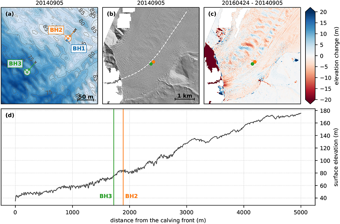
Figure 5. (a) Glacier surface topography in the vicinity of the boreholes sites in the early phase of the experiment (Arctic DEM, 2014 Sep. 5) and corresponding locations of the boreholes. The locations of BH2 and BH3 are estimated from their initial locations in July 2014 (color crosses) and the displacement of BH1 measured by continuous GPS during the corresponding time intervals. (b) Multiple illumination shaded relief map of the terminal tongue of Bowdoin Glacier from the same data. (c) Elevation change between 2014 Sep. 5 and 2016 Apr. 24 (Arctic DEM) showing generalized thinning, local thinning near the calving front, and the advection of glacier surface undulations. (d) Glacier surface topographic profile along a flow line passing near BH1 and the estimated location of BH3.

The upper borehole site (BH1, BH2) is located on a topographic high and the lower borehole site (BH3) is located in a topographic low (Figure 5a). Although this was not at all foreseen, the distance between the two boreholes is roughly equal to half the ogive wavelength. Because the surface topography of Bowdoin Glacier is overprinted by a dense crevasse pattern and abundant smaller-scale topography (Figures 1, 5a), the undulations are not obvious in the field. But in fact it could be observed during field seasons that the upper drilling site offered a more extensive view than the lower drilling site.

The lower borehole (BH3), located in a topographic dip, exhibits a warmer and faster-warming temperature profile than the upper boreholes (BH1, BH2), located on a topographic high. In light of the above observations we speculate that topographic dips may tend to localize deep crevassing. This localization of crevassing could be the result of increased longitudinal stretching due to thinner ice, increased meltwater infiltration ponding between ogives, or a combination of these two processes.

5. Conclusions

Following hot water drilling of the highly crevassed terminal tongue of Bowdoin Glacier in northwestern Greenland, we present the first continuous, multi-year temperature record from one of many marine-terminating outlet glaciers of the Greenland Ice Sheet, which have recently experienced a generalized thinning and accelerated retreat. From this record we identify potential new mechanisms that govern the englacial temperature of tidewater glaciers and thereby their viscosity.

• Temperature profiles from two drilling sites separated by 158 (2014) to 191 m (2017) differ by up to ca. 2°C indicating strong, full-depth longitudinal temperature variations in the glacier.

• Englacial warming up to 0.39°C a⁻¹, an order of magnitude above the theoretical warming from heat diffusion and viscous dissipation, indicates a deep and local heat source within the tidewater glacier.

• In the absence of visible moulins on the glacier surface, we interpret these results as the expression of latent heat released from meltwater refreezing in crevasses reaching to, or near to, the base of the glacier.

• We speculate that the localization of such deep crevasses may be controlled by preferential meltwater infiltration in topographic dips associated with ogive banding.

These results are a somewhat fortuitous conclusion of a last-minute relocation of the Bowdoin Glacier second drilling site due to unfavorable weather. They are limited by the number of sampling points (two), and need to be validated through a more systematical experiment. However, our measurements indicate a potential new mechanism for full-depth englacial warming and local ice softening that may contribute to the recently observed dynamic thinning of Greenlandic tidewater glaciers.

Data Availability Statement

The Bowdoin boreholes temperature data is available at https://doi.org/10.5281/zenodo.3695960.

Author Contributions

MF, SS, and AB set-up the Bowdoin Glacier project and first field campaign. TW and CS assembled and calibrated the borehole instruments. MF, SS, AB, and TW organized the first fieldwork and drilled the boreholes. SS processed the DGPS data. JS maintained the stations, processed the borehole data, and wrote most of the manuscript.

Funding

The current work was supported by the Swiss National Science Foundation grants no. 200020-169558 and 200021-153179/1 to MF and by the Japanese Ministry of Education, Culture, Sports, Science of Technology through the GRENE Arctic Climate Change Research Project and Arctic Challenge for Sustainability (ArCS) project. Publication fees were paid by ETH Zurich.

Conflict of Interest

The authors declare that the research was conducted in the absence of any commercial or financial relationships that could be construed as a potential conflict of interest.

Acknowledgments

We would like to thank Toku Oshima and Kim Petersen for their warm welcome in Qaanaaq, for the shooting lessons and for assistance with field preparations. Many thanks to Takanobu Sawagaki, Naoki Katayama, Jun Saito, and Shun Tsutaki for their participation in the drilling and to Evgeniy Podolskiy and Lukas Preiswerk for their precious help retrieving data from instruments and instruments from crevasses. We thank Martin Lüthi for his constructive comments and great help to interpret the data, and Eef van Dongen for insightful discussions and her help proofreading this manuscript.

References

Ahlmann, H. W. (1935). Contribution to the physics of glaciers. Geog. J. 86:97. doi: 10.2307/1786585

CrossRef Full Text | Google Scholar

Benn, D. I., Hulton, N. R., and Mottram, R. H. (2007). ‘calving laws', ‘sliding laws' and the stability of tidewater glaciers. Ann. Glaciol. 46, 123–130. doi: 10.3189/172756407782871161

CrossRef Full Text | Google Scholar

Chamberlin, T. C. (1894). Recent glacial studies in Greenland. Geol. Soc. Am. Bull. 6, 199–220. doi: 10.1130/GSAB-6-199

CrossRef Full Text | Google Scholar

Chamberlin, T. C. (1895). Glacial studies in Greenland. VII: the Redcliff peninsula. J. Geol. 3, 668–681. doi: 10.1086/607317

CrossRef Full Text | Google Scholar

Chamberlin, T. C. (1897). Glacial studies in Greenland. x. J. Geol. 5, 229–240. doi: 10.1086/607767

CrossRef Full Text | Google Scholar

Clarke, G. K. C., Nitsan, U., and Paterson, W. S. B. (1977). Strain heating and creep instability in glaciers and ice sheets. Rev. Geophys. 15:235. doi: 10.1029/RG015i002p00235

CrossRef Full Text | Google Scholar

Colgan, W., Steffen, K., McLamb, W. S., Abdalati, W., Rajaram, H., Motyka, R., et al. (2011). An increase in crevasse extent, West Greenland: hydrologic implications. Geophys. Res. Lett. 38:L18502. doi: 10.1029/2011GL048491

CrossRef Full Text | Google Scholar

Cuffey, K. M., and Paterson, W. S. B. (2010). The Physics of Glaciers. Amsterdam: Elsevier.

Google Scholar

Das, S. B., Joughin, I., Behn, M. D., Howat, I. M., King, M. A., Lizarralde, D., et al. (2008). Fracture propagation to the base of the Greenland ice sheet during supraglacial lake drainage. Science 320, 778–781. doi: 10.1126/science.1153360

PubMed Abstract | CrossRef Full Text | Google Scholar

de Q. Robin, G. (1955). Ice movement and temperature distribution in glaciers and ice sheets. J. Glaciol. 2, 523–532. doi: 10.3189/002214355793702028

CrossRef Full Text | Google Scholar

Dehecq, A., Gourmelen, N., Gardner, A. S., Brun, F., Goldberg, D., Nienow, P. W., et al. (2019). Twenty-first century glacier slowdown driven by mass loss in high mountain Asia. Nat. Geosci. 12, 22–27. doi: 10.1038/s41561-018-0271-9

CrossRef Full Text | Google Scholar

Doyle, S. H., Hubbard, B., Christoffersen, P., Young, T. J., Hofstede, C., Bougamont, M., et al. (2018). Physical conditions of fast glacier flow: 1. Measurements from boreholes drilled to the bed of Store Glacier, West Greenland. J. Geophys. Res. Earth Surf. 123, 324–348. doi: 10.1002/2017JF004529

CrossRef Full Text | Google Scholar

Enderlin, E. M., Howat, I. M., Jeong, S., Noh, M.-J., van Angelen, J. H., and van den Broeke, M. R. (2014). An improved mass budget for the Greenland ice sheet. Geophys. Res. Lett. 41, 866–872. doi: 10.1002/2013GL059010

CrossRef Full Text | Google Scholar

Glen, J. (1952). Experiments on the deformation of ice. J. Glaciol. 2, 111–114. doi: 10.1017/S0022143000034067

CrossRef Full Text | Google Scholar

Groh, A., and Horwath, M. (2016). “The method of tailored sensitivity kernels for GRACE mass change estimates,” in EGU General Assembly Conference Abstracts, Vol. 18 (Vienna), 12065.

Google Scholar

Harrington, J. A., Humphrey, N. F., and Harper, J. T. (2015). Temperature distribution and thermal anomalies along a flowline of the Greenland ice sheet. Ann. Glaciol. 56, 98–104. doi: 10.3189/2015AoG70A945

CrossRef Full Text | Google Scholar

Heid, T., and Kääb, A. (2012). Repeat optical satellite images reveal widespread and long term decrease in land-terminating glacier speeds. Cryosphere 6, 467–478. doi: 10.5194/tc-6-467-2012

CrossRef Full Text | Google Scholar

Hill, E. A., Carr, J. R., and Stokes, C. R. (2017). A review of recent changes in major marine-terminating outlet glaciers in northern Greenland. Front. Earth Sci. 4:111. doi: 10.3389/feart.2016.00111

CrossRef Full Text | Google Scholar

Iken, A., Echelmeyer, K., Harrison, W., and Funk, M. (1993). Mechanisms of fast flow in Jakobshavns Isbræ, West Greenland: Part I. Measurements of temperature and water level in deep boreholes. J. Glaciol. 39, 15–25. doi: 10.1017/S0022143000015689

CrossRef Full Text | Google Scholar

Jania, J., Mochnacki, D., and Ga̧dek, B. (1996). The thermal structure of Hansbreen, a tidewater glacier in southern Spitsbergen, Svalbard. Polar Res. 15, 53–66. doi: 10.1111/j.1751-8369.1996.tb00458.x

CrossRef Full Text | Google Scholar

Jouvet, G., Weidmann, Y., Kneib, M., Detert, M., Seguinot, J., Sakakibara, D., et al. (2018). Short-lived ice speed-up and plume water flow captured by a VTOL UAV give insights into subglacial hydrological system of Bowdoin Glacier. Remote Sens. Environ. 217, 389–399. doi: 10.1016/j.rse.2018.08.027

CrossRef Full Text | Google Scholar

Jouvet, G., Weidmann, Y., Seguinot, J., Funk, M., Abe, T., Sakakibara, D., et al. (2017). Initiation of a major calving event on the Bowdoin Glacier captured by UAV photogrammetry. Cryosphere 11, 911–921. doi: 10.5194/tc-11-911-2017

CrossRef Full Text | Google Scholar

Kanna, N., Sugiyama, S., Ohashi, Y., Sakakibara, D., Fukamachi, Y., and Nomura, D. (2018). Upwelling of macronutrients and dissolved inorganic carbon by a subglacial freshwater driven plume in Bowdoin Fjord, northwestern Greenland. J. Geophys. Res. Biogeo. 123, 1666–1682. doi: 10.1029/2017JG004248

CrossRef Full Text | Google Scholar

Khan, S. A., Aschwanden, A., Bjørk, A. A., Wahr, J., Kjeldsen, K. K., and Kjær, K. H. (2015). Greenland ice sheet mass balance: a review. Rep. Prog. Phys. 78:046801. doi: 10.1088/0034-4885/78/4/046801

PubMed Abstract | CrossRef Full Text | Google Scholar

Khan, S. A., Wahr, J., Bevis, M., Velicogna, I., and Kendrick, E. (2010). Spread of ice mass loss into northwest Greenland observed by GRACE and GPS. Geophys. Res. Lett. 37:L06501. doi: 10.1029/2010GL042460

CrossRef Full Text | Google Scholar

Krabill, W., Abdalati, W., Frederick, E., Manizade, S., Martin, C., Sonntag, J., et al. (2000). Greenland ice sheet: high-elevation balance and peripheral thinning. Science 289, 428–430. doi: 10.1126/science.289.5478.428

PubMed Abstract | CrossRef Full Text | Google Scholar

Lüthi, M., Funk, M., Iken, A., Gogineni, S., and Truffer, M. (2002). Mechanisms of fast flow in Jakobshavns Isbræ, West Greenland: part III. Measurements of ice deformation, temperature and cross-borehole conductivity in boreholes to the bedrock. J. Glaciol. 48, 369–385. doi: 10.3189/172756502781831322

CrossRef Full Text | Google Scholar

Lüthi, M. P., Ryser, C., Andrews, L. C., Catania, G. A., Funk, M., Hawley, R. L., et al. (2015). Heat sources within the Greenland ice sheet: dissipation, temperate paleo-firn and cryo-hydrologic warming. Cryosphere 9, 245–253. doi: 10.5194/tc-9-245-2015

CrossRef Full Text | Google Scholar

McMillan, M., Leeson, A., Shepherd, A., Briggs, K., Armitage, T. W. K., Hogg, A., et al. (2016). A high-resolution record of Greenland mass balance. Geophys. Res. Lett. 43, 7002–7010. doi: 10.1002/2016GL069666

CrossRef Full Text | Google Scholar

Meier, M. F., and Post, A. (1987). Fast tidewater glaciers. J. Geophys. Res. 92:9051. doi: 10.1029/JB092iB09p09051

CrossRef Full Text | Google Scholar

Moon, T., Joughin, I., and Smith, B. (2015). Seasonal to multiyear variability of glacier surface velocity, terminus position, and sea ice/ice mélange in northwest Greenland. J. Geophys. Res. Earth Surf. 120, 818–833. doi: 10.1002/2015JF003494

CrossRef Full Text | Google Scholar

Moon, T., Joughin, I., Smith, B., and Howat, I. (2012). 21st-century evolution of Greenland outlet glacier velocities. Science 336, 576–578. doi: 10.1126/science.1219985

PubMed Abstract | CrossRef Full Text | Google Scholar

Nye, J. F. (1953). The flow law of ice from measurements in glacier tunnels, laboratory experiments and the Jungfraufirn borehole experiment. Proc. R. Soc. London Ser. A 219, 477–489. doi: 10.1098/rspa.1953.0161

CrossRef Full Text | Google Scholar

Nye, J. F. (1955). Comments on Dr. Loewe's letter and notes on crevasses. J. Glaciol. 2, 512–514. doi: 10.1017/S0022143000032652

CrossRef Full Text | Google Scholar

Phillips, T., Rajaram, H., Colgan, W., Steffen, K., and Abdalati, W. (2013). Evaluation of cryo-hydrologic warming as an explanation for increased ice velocities in the wet snow zone, Sermeq Avannarleq, West Greenland. J. Geophys. Res. Earth Surf. 118, 1241–1256. doi: 10.1002/jgrf.20079

CrossRef Full Text | Google Scholar

Phillips, T., Rajaram, H., and Steffen, K. (2010). Cryo-hydrologic warming: a potential mechanism for rapid thermal response of ice sheets. Geophys. Res. Lett. 37:L20503. doi: 10.1029/2010GL044397

CrossRef Full Text | Google Scholar

Podolskiy, E. A., Genco, R., Sugiyama, S., Walter, F., Funk, M., Minowa, M., et al. (2017). Seismic and infrasound monitoring of Bowdoin Glacier, Greenland, low temperature science. Low Temp. Sci. 75, 15–36.

Google Scholar

Podolskiy, E. A., Sugiyama, S., Funk, M., Walter, F., Genco, R., Tsutaki, S., et al. (2016). Tide-modulated ice flow variations drive seismicity near the calving front of Bowdoin Glacier, Greenland. Geophys. Res. Lett. 43, 2036–2044. doi: 10.1002/2016GL067743

CrossRef Full Text | Google Scholar

Pritchard, H. D., Arthern, R. J., Vaughan, D. G., and Edwards, L. A. (2009). Extensive dynamic thinning on the margins of the Greenland and Antarctic ice sheets. Nature 461, 971–975. doi: 10.1038/nature08471

PubMed Abstract | CrossRef Full Text | Google Scholar

Rignot, E., and Kanagaratnam, P. (2006). Changes in the velocity structure of the Greenland ice sheet. Science 311, 986–990. doi: 10.1126/science.1121381

PubMed Abstract | CrossRef Full Text | Google Scholar

Ryser, C. (2014). Cold ice in an alpine glacier and ice dynamics at the margin of the Greenland ice sheet. (PhD thesis). Zürich: ETH Zürich.

Google Scholar

Ryser, C., Lüthi, M. P., Andrews, L. C., Catania, G. A., Funk, M., Hawley, R., et al. (2014a). Caterpillar-like ice motion in the ablation zone of the Greenland ice sheet. J. Geophys. Res. Earth Surf. 119, 2258–2271. doi: 10.1002/2013JF003067

CrossRef Full Text | Google Scholar

Ryser, C., Lüthi, M. P., Andrews, L. C., Hoffman, M. J., Catania, G. A., Hawley, R. L., et al. (2014b). Sustained high basal motion of the Greenland ice sheet revealed by borehole deformation. J. Glaciol. 60, 647–660. doi: 10.3189/2014JoG13J196

CrossRef Full Text | Google Scholar

Sakakibara, D., and Sugiyama, S. (2018). Ice front and flow speed variations of marine-terminating outlet glaciers along the coast of Prudhoe Land, northwestern Greenland. J. Glaciol. 64, 300–310. doi: 10.1017/jog.2018.20

CrossRef Full Text | Google Scholar

Seddik, H., Greve, R., Sakakibara, D., Tsutaki, S., Minowa, M., and Sugiyama, S. (2019). Response of the flow dynamics of Bowdoin Glacier, northwestern Greenland, to basal lubrication and tidal forcing. J. Glaciol. 65, 225–238. doi: 10.1017/jog.2018.106

CrossRef Full Text | Google Scholar

Seguinot, J., Rogozhina, I., Stroeven, A. P., Margold, M., and Kleman, J. (2016). Numerical simulations of the Cordilleran ice sheet through the last glacial cycle. Cryosphere 10, 639–664. doi: 10.5194/tc-10-639-2016

CrossRef Full Text | Google Scholar

Shapero, D. R., Joughin, I. R., Poinar, K., Morlighem, M., and Gillet-Chaulet, F. (2016). Basal resistance for three of the largest Greenland outlet glaciers. J. Geophys. Res. Earth Surf. 121, 168–180. doi: 10.1002/2015JF003643

CrossRef Full Text | Google Scholar

Sugiyama, S., Sakakibara, D., Matsuno, S., Yamaguchi, S., Matoba, S., and Aoki, T. (2014). Initial field observations on Qaanaaq ice cap, northwestern Greenland. Ann. Glaciol. 55, 25–33. doi: 10.3189/2014AoG66A102

CrossRef Full Text | Google Scholar

Sugiyama, S., Sakakibara, D., Tsutaki, S., Maruyama, M., and Sawagaki, T. (2015). Glacier dynamics near the calving front of Bowdoin Glacier, northwestern Greenland. J. Glaciol. 61, 223–232. doi: 10.3189/2015JoG14J127

CrossRef Full Text | Google Scholar

Tsutaki, S., Sugiyama, S., Sakakibara, D., Aoki, T., and Niwano, M. (2017). Surface mass balance, ice velocity and near-surface ice temperature on Qaanaaq ice cap, northwestern Greenland, from 2012 to 2016. 58:181–192. doi: 10.1017/aog.2017.7

CrossRef Full Text | Google Scholar

Tsutaki, S., Sugiyama, S., Sakakibara, D., and Sawagaki, T. (2016). Surface elevation changes during 2007–13 on Bowdoin and Tugto glaciers, northwestern Greenland. J. Glaciol. 62, 1083–1092. doi: 10.1017/jog.2016.106

CrossRef Full Text | Google Scholar

van der Veen, C. J. (2007). Fracture propagation as means of rapidly transferring surface meltwater to the base of glaciers. Geophys. Res. Lett. 34:L01501. doi: 10.1029/2006GL028385

CrossRef Full Text | Google Scholar

Walter, J. I., Box, J. E., Tulaczyk, S., Brodsky, E. E., Howat, I. M., Ahn, Y., et al. (2012). Oceanic mechanical forcing of a marine-terminating Greenland glacier. Ann. Glaciol. 53, 181–192. doi: 10.3189/2012AoG60A083

CrossRef Full Text | Google Scholar

Walters, R. A. (1989). Small-amplitude, short-period variations in the speed of a tide-water glacier in south-central Alaska, U.S.A. Ann. Glaciol. 12, 187–191. doi: 10.3189/S0260305500007175

CrossRef Full Text | Google Scholar