Re-evaluation of the Power of the Mann-Kendall Test for Detecting Monotonic Trends in Hydrometeorological Time Series

The Mann-Kendall (MK) statistical test has been widely applied in the trend detection of the hydrometeorological time series. Previous studies have mainly focused on the null hypothesis of “no trend” or the “Type I Error.” However, few studies address the capability of the MK test to successfully recognize the trends. In some cases, especially when the trend test is jointly applied with hydropower station design, flood risk assessment, and water quality evaluation, the “Type II error” is equally important and should not be neglected. To cope with this problem, we carry out Monte Carlo simulations and the results indicate that in addition to the significance level and the sample length, the MK test power has a close relationship with the sample variance and the magnitude of the trend. For a given time series with fixed length, the power of the MK test increases as the slope increases and declines with increasing sample variance. A deterministic relationship between the slope and the standard deviation of the white noise that can be used for evaluating the power of the MK test has also been detected. Furthermore, we find that a positive autocorrelation contained in the time series will increase both the Type I and the Type II errors due to the enlargement of the variance in the MK statistics. Finally, we recommend that researchers slightly increase the significance level and lengthen the time series sample to improve the power of the MK test in future studies.

Introduction

Stationarity has drawn much attention since the publication of the article in the journal Science by Milly et al. (2008), which announced “Stationarity is dead.” As one of the co-authors, Hirsch (2011) argued that non-stationarity came from many other sources other than climate change, some of which may even have more significant influences. It was noted by Bayazit (2015) that the impacts of climate change and anthropogenic activities on river basins and low-frequency climatic variability were the main reasons for non-stationarity. Milly et al. (2015) stated that non-stationary conditions can come from local human activities (such as land use and land cover change, land drainage, dams, diversions, water withdrawals, and groundwater depletion) and anthropogenic climate change (ACC), whose influences are extensive, imperceptible, and growing (Shao et al., 2016, 2018; Wang et al., 2017; Zhu et al., 2018; Bai et al., 2019; Wang K. et al., 2019; Yu et al., 2019).

Many studies worldwide have investigated anthropogenic changes in the form of gradual trends or abrupt changes in the time series of hydrological variables (Serinaldi et al., 2018). Statistical hypothesis tests together with deterministic hydrological models (Kan et al., 2017a,b, 2018), climate models, and expert opinion are undoubtedly indispensable tools for trend recognition, as chaos theory stats that even a deterministic system may perform unpredictably (Yevjevich, 1974; Milly et al., 2015).

The Mann-Kendall (MK) statistical test (Mann, 1945; Kendall, 1975), a rank-based non-parametric method, has been widely used for detecting trends in hydrometeorological time series such as groundwater (Helsel and Hirsch, 1992), water quality (Hirsch et al., 1982; Hirsch and Slack, 1984; Hipel et al., 1988; Burn et al., 2012), streamflow (Douglas et al., 2000; Yue et al., 2002b; Cong et al., 2010; Sang et al., 2014; Serinaldi et al., 2018), lake level (Chebana et al., 2017), temperature, and precipitation (Lettenmaier et al., 1994; Sang et al., 2014; Wang S. et al., 2019). Compared to parametric tests (e.g., regression coefficient test), non-parametric tests (e.g., the MK test and Spearman' rho test) have no requirements of homoscedasticity or prior assumptions on the distribution of the data sample (Önöz and Bayazit, 2003) and are less sensitive to outliers (Hamed and Ramachandra Rao, 1998; Hamed, 2007). As the MK test statistic is determined by the ranks and sequences of time series rather than the original values, it is robust when dealing with non-normally distributed data, censored data, and time series with missing values (Hirsch and Slack, 1984), which are commonly encountered in hydrometeorological time series (Duan et al., 2018, 2019; Gao et al., 2018, 2019; Dong et al., 2019).

Although the MK test is relatively effective and robust, it still has a basic requirement that the data should be independent (Wasserstein et al., 2019). In other words, the MK test is not robust against serial correlation, which may be statistically significant in some hydrological and climate time series (Tian et al., 2018a,b). The positive serial correlation contained in the data will lead to over-rejection of the null hypothesis of no trend (Cox and Stuart, 1955), which has long been discussed and well-documented (Kulkarni and Von Storch, 1995; Von Storch and Navarra, 1995; Hamed and Ramachandra Rao, 1998; Yue and Wang, 2002; Yue et al., 2002a, 2003; Bayazit and Önöz, 2007; Bayazit, 2015). Two main approaches have been proposed to eliminate the influence of serial correlation, the first is applying pretreatment to the data, and the second is modifying the MK test to account for serial correlation (Hamed, 2008). Since Von Storch and Navarra (1995) and Kulkarni and Von Storch (1995) quantified the influence of serial correlation on the MK test by Monte Carlo simulation and proposed the “pre-whitening (PW)” procedure to eliminate it, PW has been widely applied. Similar to other hypothesis tests, the MK test also has two types of errors, rejecting H0 when there is no trend (Type I error) and accepting H0 when there is a true trend (Type II error). PW can significantly reduce the Type I error caused by serial correlation but will also increase the risk of Type II error, because the presence of a trend alters the estimate of the magnitude of serial correlation and the power of MK will deteriorate after PW, as Yue et al. (2002b) stated. Yue et al. (2002b, 2003) advocated that a trend first be removed in a series before the PW procedure, which is known as the “trend free pre-whitening (TFPW)” approach, as well as its modified version TFPWcu from Serinaldi and Kilsby (2016). Hamed (2009) suggested the correction of bias in the correlation coefficient to enhance the effectiveness of PW. The mutual interaction between serial correlation and trend makes this quite complicated and brings extensive debate on how to apply PW properly (Yue and Wang, 2002; Bayazit and Önöz, 2004; Zhang and Zwiers, 2004). Yue and Wang (2002) and Bayazit and Önöz (2007) suggest that PW should be avoided when the sample size and the magnitude of the trend slope are large. Based on another thought known as effective sample size, which was proposed by Bayley and Hammersley (1946) and first applied by Lettenmaier (1976) with Spearman's rho test and the Mann-Whitney test, Hamed and Ramachandra Rao (1998) proposed a variance correction approach for the MK test, as Yue et al. (2002b) stated that serial correlation influences the MK test by altering the variance in the estimate of the statistic. Eventually, the debate around different approaches dealing with serial correlation and trend becomes a mathematical game and compromises the balance between the significance and power of the MK test, and the only thing that matters is which error is more unacceptable in specific cases.

Stationarity and non-stationarity elements coexist in most hydrometeorological systems, and there are always time-invariant mechanisms in hydrological systems, as Montanari and Koutsoyiannis (2014) argued. Hypothesis tests such as the MK test are utilized to recognize the non-stationary components, which appear deterministic, apart from uncertain and random stationary components. For a specific trend test, the capability of recognizing a significant trend depends on whether the non-stationary (trend) components are strong enough to shine through the stationary (random) components, which should be considered when the power of a test is assessed. What should be noted is that for various hydrometeorological variables, there can be vast differences in the magnitudes of the involved uncertainties. The magnitude can be very small with annual maximum or minimum temperature data, or be quite large with annual runoff time series, as implied by the variance in the data samples. Even though thousands of trend detection studies have been published, most of them only concentrate on the null hypothesis of “no trend,” Vogel et al. (2013) argued, while little or no attention is paid to the power. The above-reviewed articles have little consideration of the magnitude of the uncertainty when assessing the power of the MK test.

The objectives of this study are as follows: (a) to explore the power of the MK test against different uncertainty levels; (b) to investigate the effect of serial correlation on the Type I error of the MK test against different uncertainty levels; (c) to document the effect of serial correlation on the power of the MK test against different uncertainty levels; and (d) to propose some reasonable suggestions in using the MK test in future studies.

Methodology

Description of the MK Test

The Mann–Kendall trend test (Mann, 1945; Kendall, 1975) is based on the correlation between the ranks and sequences of a time series. For a given time series {X_i, i = 1, 2…, n}, the null hypothesis H0 assumes it is independently distributed, and the alternative hypothesis H1 is that there exists a monotonic trend. The test statistic S is given by:

$\begin{array}{ll}S={{\displaystyle \sum }}_{i=1}^{n-1}{{\displaystyle \sum }}_{j=i+1}^n\text{sgn}({\text{X}}_j-{\text{X}}_i)& (1)\end{array}$

where X_i and X_j are the values of sequence i, j; n is the length of the time series and

$\begin{array}{ll}\text{sgn}(\theta )=\{\begin{array}{c}1if\theta >0\\ 0if\theta =0\\ -1if\theta <0\end{array}& (2)\end{array}$

Mann (1945) and Kendall (1975) have documented that the statistic S is approximately normally distributed when n ≥ 8, with the mean and the variance of statistics S as follows:

$\begin{array}{ll}E(S)=0& (3)\end{array}$

$\begin{array}{ll}V(S)=\frac{n(n-1)(2n+5)-{\displaystyle {\sum }_{i=1}^m}{T}_{i}i(i-1)(2i+5)}{18}& (4)\end{array}$

where T_i is the number of data in the tied group and m is the number of groups of tied ranks. The standardized test statistic Z is computed by

$\begin{array}{ll}Z=\{\begin{array}{c}\frac{S-1}{\sqrt{V(S)}}S>0\\ 0S=0\\ \frac{S+1}{\sqrt{V(S)}}S<0\end{array}& (5)\end{array}$

The standardized MK statistic Z follows the standard normal distribution with E(Z) = 0 and V(Z) = 1, and the null hypothesis is rejected if the absolute value of Z is larger than the theoretical value Z_1−α/2 (for two-tailed test) or Z_1−α (for one-tailed test), where α is the statistical significance level concerned.

Synthetic Study Using Monte Carlo Simulation

A synthetic study using Monte Carlo simulation is carried out in this study. Monte Carlo simulation has been extensively utilized to assess the effect of serial correlation on statistical hypothesis tests (Kulkarni and Von Storch, 1995; Yue and Wang, 2002; Yue et al., 2002a,b) and the power of statistical hypothesis tests (Hirsch et al., 1982; Lettenmaier, 1988; Yue and Pilon, 2004; Yue and Wang, 2004; Sang et al., 2014). In this study, the time series with trend is generated by

$\begin{array}{ll}{Y}_t=T_t+B+N_t& (6)\end{array}$

where N_t is white noise, B is a constant parameter, and T_t can be defined as:

$\begin{array}{ll}{T}_t=At& (7)\end{array}$

where A is the slope value. For time series Y_t, T_t + B represents the trend term, and N_t represents the random term.

The serial correlation is presented by an autoregressive process of first order, the AR(1) process, the same as Kulkarni and Von Storch (1995) used.

$\begin{array}{ll}{X}_t=\rho X_{t-1}+N_t& (8)\end{array}$

where ρ is the lag-1 autocorrelation coefficient and N_t is white noise. What else has been taken into consideration is the variance in white noise, named power spectral density (PSD), because it is the main influencing factor of the variance in a given sample, which to some extent can reflect the uncertainty.

For a time series in which the trend term and correlation term coexist, the variance in the sample is determined by three factors: PSD, the length of the time series and the magnitude of the trend value. The influence of the length of the time series and the magnitude of the trend value are reflected in the trend term. For time series Y_t = At + B (t = 1 ~ n), the variance is

$\begin{array}{ll}Variance\text{\_}Trend=\frac{n^2+11}{12}{A}^2& (9)\end{array}$

Based on the abovementioned equation, the variance from the trend term will be quite small with limited slope value A. Therefore, the influence from the trend term to the magnitude of sample variance is limited, and the variance will be close to the PSD of white noise. This factor will be evaluated in the following study using gauged data.

Evaluation of the Power of the MK Test

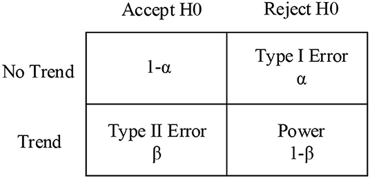
For the statistical hypothesis test, the significance level α is the probability of rejecting the null hypothesis when there is no trend. The power of the MK test is the probability of rejecting the null hypothesis, 1 − β, when there is a trend contained in the data sample (see Figure 1).

FIGURE 1

Figure 1. Probability matrix for the MK test, with the null hypothesis H0 showing no trend.

For samples with a specific length and significance level, the power and the size of the confidence interval are contradictory (see Figure 2), which means that a small significance level (probability of Type I error) will reduce the power of the test. While applying the hypothesis test, the Type I error can be controlled by the significance level α, but the Type II error depends on the sample length in addition to α. In specific cases, the Type II error should also be controlled in addition to reducing the Type I error, especially when the MK test is associated with hydropower station design, flood risk assessment, and water quality evaluation. The power seems more important in such situations, as Vogel et al. (2013) argued, because the power informs us about the likelihood of whether society is prepared to accommodate and respond to such trends. Delaying action should be made when designing flood control engineering if there are no sufficient historical data (Rehan and Hall, 2014).

FIGURE 2

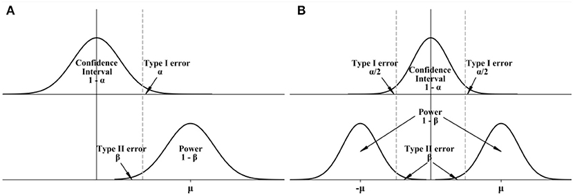
Figure 2. Relationship of confidence interval, critical region and power for (A) one-tailed test and (B) two-tailed test.

In Monte Carlo simulation experiments, the power of the MK test can be estimated by the following equation, as Yue et al. (2002a) and Yue and Pilon (2004) stated:

$\begin{array}{ll}Power=\frac{N_{rej}}{N}& (10)\end{array}$

where N is the total number of experiments and N_rej is the number of experiments whose observed value is larger than the critical value (see Figure 2).

Results and Discussion

Power of the MK Test Against PSD

Monte Carlo simulations under various combinations of the trend term and the random term are conducted to observe the power of the MK test against the PSD of white noise. In the first simulation experiment, the sample length is set to 50, 100, 200, and 400. The PSD of white noise varies from 10⁻⁴ to 10⁴ with a multiplier of 10^0.08, and the value of the slope varies from 10⁻³ to 10⁻¹ with a multiplier of 10^0.02. Therefore, we can obtain a square matrix with a size of 101 × 101, and each element represents a combination of the PSD and the value of the slope. The serial correlation is not taken into consideration in this part and therefore is set to zero. With each combination of PSD and slope, 1,000 time series are generated with the abovementioned method, and the rejection number of the MK test is recorded and demonstrated in a heat map (see Figure 3). The dashed line is shown as a boundary, the left of which the rejection number is larger than 950 and the right is <950. The solid line is the line on which the variance of the trend term is equal to the PSD of white noise.

FIGURE 3

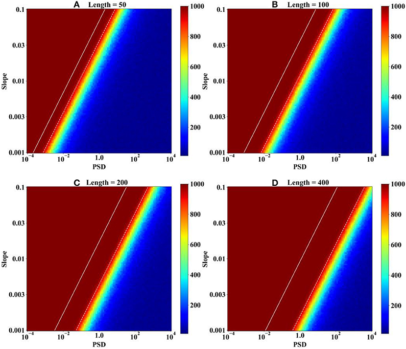
Figure 3. Heat map of the rejection number under different combinations of PSD and slope. (A) Sample lengths = 50; (B) sample lengths = 100; (C) sample lengths = 200; and (D) sample lengths = 400.

It is obvious that for a given sample length, the rejection number, which can represent the power of the MK test, increases as the slope increases and decreases with increasing PSD. A clearly linear boundary, on the left of which the rejection number is larger than 950 and on the right is <950, divides the space into a high rejection region and a low rejection region. The equation of those dashed lines can be estimated by multiple simulations, which are:

$\begin{array}{ll}\{\begin{array}{c}\begin{array}{c}A=\sqrt{PSD}\times 10^{-1.44}=SD\times 10^{-1.44}n=50\\ A=\sqrt{PSD}\times 10^{-1.92}=SD\times 10^{-1.92}n=100\end{array}\\ A=\sqrt{PSD}\times 10^{-2.36}=SD\times 10^{-2.36}n=200\\ A=\sqrt{PSD}\times 10^{-2.80}=SD\times 10^{-2.80}n=400\end{array}& (11)\end{array}$

where A is the slope value and SD is the standard deviation of the white noise.

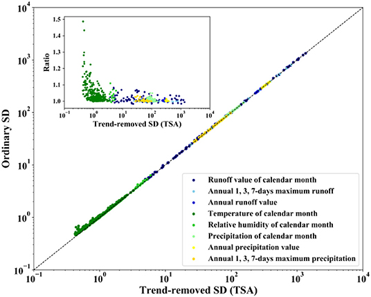
What those equations interpreted is that there is a deterministic relation between the slope and the PSD of white noise, which can be used for evaluating the power of the MK test. When a sample of hydrometeorological time series is collected and analyzed by the MK test, the magnitude of the slope beyond which the test is effective can be estimated by the length of the sample and the PSD or SD of the white noise. The paradox is, as mentioned above, that the variance in the sample data is not exactly equal to the PSD of the white noise because of the influence of the trend term. The solid line in Figure 3 indicates that the influence of the trend term is increasing with the increase in the length of the sample and the magnitude of the trend, which could be the determinant of the sample variance if the ratio of the slope value to the SD of white noise is large enough. However, in actual situations, the coexistence situation of the slope value and the variance in the sample are limited: the situation in which a large slope value and white noise with a small PSD coexist in one sample is rare, and the influence of the trend on the variance in the sample is finite. To verify this, 11 variables extracted from 30 hydrologic gauges and 9 variables extracted from 20 meteorological stations, i.e., a total of 510 samples with the length of each sample equal to 55, are analyzed. The Theil–Sen approach (TSA) proposed by Theil (1950) and Sen (1968) is used to estimate the trend. The ordinary SD of the sample and the trend-removed SD, which can be assumed as the SD of the white noise, are calculated and shown in Figure 4 using logarithmic coordinates. The trends of the sample data are removed by

$\begin{array}{l}{Y}_t^{\prime }=Y_t-T_t=Y_t-At\end{array}$

As Figure 4 shows, the ordinary SD values and the trend-removed SD values are almost the same, as all the data points are close to the dashed line whose gradient is 1. To better illustrate this, the variation in the ratio of the two SDs is shown in the subfigure of Figure 4. The influence of the trend on the variance decreases with increasing PSD of white noise. For the 510 samples analyzed in this study, the difference between the variance in the sample and the PSD of white noise is quite small. Therefore, the magnitude of the slope beyond which the MK test is effective can be roughly estimated by the length and the variance in the sample, which is practically meaningful.

FIGURE 4

Figure 4. Comparison of ordinary SD and trend-removed SD.

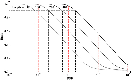
The power of the MK test is a monotonically increasing function of the sample length, as shown in Figure 3 and more obviously demonstrated in Figure 5. For example, the rejection ratios are ~0.98, 0.8, 0.6, and 0.4 when the PSD equals 1 and the sample lengths are 400, 200, 100, and 50, respectively, and the ratios will increase to 0.1, 0.04, 0.03, and 0.025, respectively, when the PSDs are equal to 100. The fact should be noted is that the rejection ratios in this figure cannot perfectly represent the power of the MK test because, in this simulation, the scope of the slope value is limited; however, it is still meaningful and interpretive. From another perspective, Figure 5 indicates that if the desired power is specified, the way to resist the PSD for maintaining the power is to extend the sample length to a required minimum value. For a power of 0.9, represented in Figure 5 as a black dashed line, the minimum sample length required will be 50 if the variance in the sample is ~0.08, and the required length will increase to 400 if the variance in the sample is 1.7. However, those values largely depend on the evaluation method of the power of the test. As mentioned in the above paragraphs, the scope of the slope values is limited from 0.001 to 0.1 in this simulation, which means that the ratios in Figure 5 are incomplete expressions of the power of the MK test.

FIGURE 5

Figure 5. The rejection ratio of the MK test against the PSD of white noise.

Therefore, a comparison of the distributions of test statistics against different PSDs is made and shown in Figure 6. In each subfigure, 10,000 time series are simulated. Figure 6A shows the distribution of the MK test statistic where there is no trend; Figure 6B shows the distribution of the MK test statistic against different PSDs where the slope value varies from 0.001 to 0.1; Figure 6C shows the distribution of the MK test statistic against different PSDs where the slope values vary from 10⁻⁵ to 10⁻² × SD; and Figure 6D shows the distribution of the MK test statistic against different PSDs where the slope values vary from 10⁻⁵ to 10⁻¹ × SD.

FIGURE 6

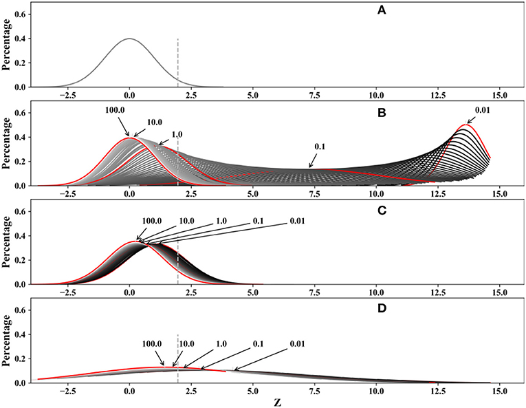
Figure 6. Comparison of the distribution of test statistics against different PSDs with sample lengths equal to 100. The critical region is marked by the dashed line. (A) Slope value = 0; (B) slope value = 0.001 – 0.1; (C) slope value = 10⁻⁵ to 10⁻² × SD; and (D) slope value = 10⁻⁵ to 10⁻¹ × SD.

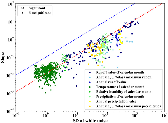
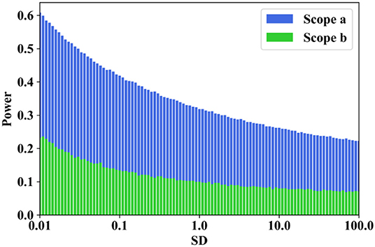
Figure 6B indicates that the difference between the power of the MK test under a distinct PSD of white noise can be quite large when the scope of the slope value is 0.001 to 0.1. In addition, the variance in the MK test statistics is significantly large when the sample variance is between 0.1 and 1.0. This can be explained by Equation (11). Taking samples whose SDs are equal to 1 as examples, the rejection rate will be close to 1 when the slope value is larger than 10^−1.92 according to Equation (11). The statistics become quite sensitive to the slope value when it is larger than 10^−1.92, and the distribution type is no longer normal. Contrastive simulations are conducted where the scope of the slope values are from 10⁻⁵ to 10⁻¹ × SD and from 10⁻⁵ to 10⁻² × SD, which means the upper limit of the slope is controlled by the PSD of the white noise. The results are shown in Figures 6C,D. These two subfigures signify that no matter how large the PSD of the white noise is, the power of the test could always be large enough if the upper scope of the slope is set with a sufficiently high value. Therefore, when evaluating the power of the MK test, it is unreasonable to consider the power of the MK test with a fixed scope of slope or even neglecting the scope of slope; however, this factor is neglected by most of the existing studies. A variable upper limit associated with the PSD of white noise should be adopted to assess the power of the MK test. The reason is that in practice, the magnitude of the slope would be limited in a time series with a specific PSD. The 510 samples used above are performed as a case study of this situation, as shown in Figure 7. The slope values are estimated by TSA and then removed to obtain the SD of the white noise. Two dashes are drawn as references: the blue dash is A = 10⁻¹ × SD, and the red dash is A = 10^−1.92 × SD, which is slightly off the theoretical value of Equation (11) as the sample length is 55. This result might be caused by the influence of serial correlation or the approach used for estimating the slope. All the significant results are located between the two lines, and the blue line is chosen as the upper limit analyzed in Figure 6D. Rejection rates in these two situations were recorded, and the results are shown in Figure 8, which indicate that the power of the MK test varies from 0.24 to 0.07 when the upper limit of the slope value is set as 10⁻² × SD (Scope b) and will increase to 0.61 and 0.22 when the upper limit of the slope value is set to 10⁻¹ × SD (Scope a).

FIGURE 7

Figure 7. Slope values against the SD of white noise.

FIGURE 8

Figure 8. Power of the MK test against different SD values and different slope scopes.

Generally, for a given population, the power of a statistical hypothesis test is just a function of the sample length if the significance level is set. For tests utilized for seeking trends in time series with different variances, it is meaningful to evaluate the power by separating it with the different conditions of the sample variance because the sample variance can always be calculated and is an unbiased estimation of the variance in the population. Even though it is difficult to evaluate the power of the general population, it becomes operable when the population of hydrometeorological variables is classified according to variance, as discussed above.

Effect of Serial Correlation on the Type I Error of the MK Test Against PSD

As stated by Kulkarni and Von Storch (1995), Von Storch and Navarra (1995), and Yue et al. (2002b), the existence of positive serial correlation will increase the Type I error of the MK test. To investigate the influence of serial correlation on the MK test against different PSDs and sample lengths, two simulation experiments were conducted with sample lengths set as 50 and 100, the PSD varying from 10⁻⁴ to 10⁴ and serial correlations varying from 0 to 0.9. For each combination of serial correlation and the PSD, 1,000 simulations were conducted. As the significance level is set to 0.05, the theoretical value of the rejection rate should be 0.05 when there is no trend. However, as shown in Figure 9, the rejection rate increases as the serial correlation increases and will be ~0.15 when the serial correlation is 0.3, which is the same as the result of Kulkarni and Von Storch (1995) Additionally, it indicates that the rejection rate remains unchanged with various PSDs, which means the effect of serial correlation on Type I error is the same for time series with different variances. Little differences in rejection rates can be observed between the two subfigures, and the rejection rate in Figure 9B is slightly higher than that in Figure 9A. The difference may not come from the variation in sample lengths but from the fact that the actual serial correlation value is not exactly the one added into the time series through Equation (8), which is more obvious with a short sample lengths. By Monte Carlo simulation, we find that the serial correlations within different time series added through Equation (8) show negative skewness rather than a normal distribution. The mean value becomes larger and the coefficient of variation decreases with increasing sample length. This should be the source of the slight differences in rejection rates between various sample lengths.

FIGURE 9

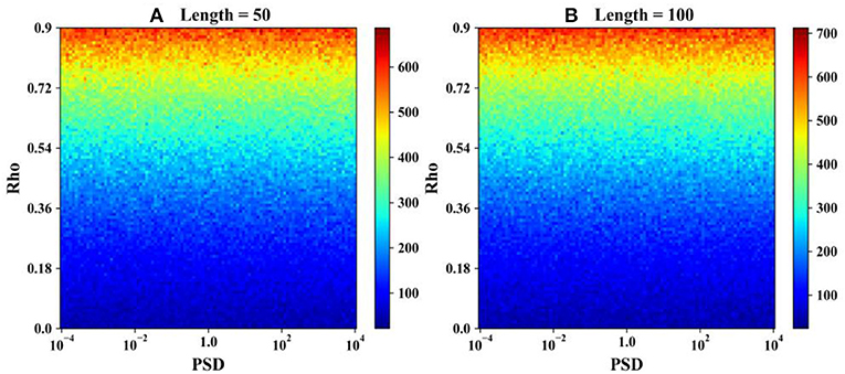
Figure 9. Heat map of the rejection number under different serial correlation coefficients. (A) Sample lengths = 50 and (B) sample lengths = 100.

Figure 10 shows the distributions of the standardized MK statistics against different serial correlations, while no trend exists in the time series. In this simulation, the sample lengths are both set as 100, the PSDs of white noise are both set as 1, and the autocorrelation coefficients are 0 and 0.9. As illustrated by the box-plot and the violin-plot, neither the asymptotic normality nor the mean of the MK statistic changes with the serial correlation. The variance in the standardized MK statistics increases from 1 to 13.2, while the serial correlation increases from 0 to 0.9. This result explains why the existence of positive serial correlation causes an increase in rejection rates when there are no trends, in other words, the probability of Type I error. The positive serial correlation increases the variance in the standardized MK statistics and keeps the mean value of the standardized MK statistics as zero; therefore, the probability that statistics fall into the critical region is increasing.

FIGURE 10

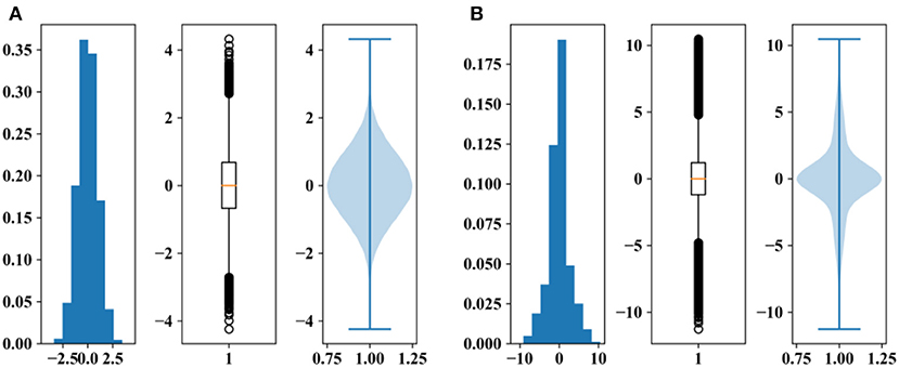
Figure 10. Distributions of the standardized MK statistics with different autocorrelation coefficients. (A) Autocorrelation coefficient = 0 and (B) autocorrelation coefficient = 0.9.

Effect of Serial Correlation on the Power of the MK Test Against PSD

To investigate the effect of serial correlation on the power of the MK test against PSD, another two simulation experiments were conducted, the first one with fixed PSD and the second one with fixed slope value, and the results are shown in Figures 11, 12, respectively. Figure 11 shows that for a specific PSD and slope value, the variations in the rejection rate show different patterns with increasing serial correlations. Taking Figure 11A as an example, the rejection rate increases with serial correlation when the slope value is 0.001, while it decreases with increasing serial correlation when the slope value is 0.01. Therefore, for time series with specific PSD values, the effect of serial correlation on the power of the MK test will be different from variable slope values. This is contradictory to previous studies that suggested that the positive serial correlation makes the MK test overestimate the significance of the trend. For time series with large slope values, the effect would be negative with the existence of serial correlation. With increasing PSD, the threshold of the slope value increases, as shown in Figure 11B.

FIGURE 11

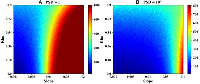
Figure 11. Heat map of the rejection rate with different combinations of slope values and serial correlation values, where the sample length is 100 and PSD values are equal to 1 and 100 respectively. (A) PSD = 1 and (B) PSD = 10².

FIGURE 12

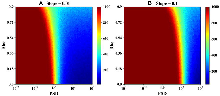
Figure 12. Heat maps of the rejection rate with different combinations of PSD values and serial correlation values, where the sample length is 100 and the slope values are equal to 0.01 and 0.1, respectively. (A) Slope value = 0.01 and (B) slope value = 0.1.

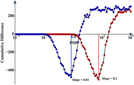
The same law can be observed from Figure 12, which indicates that with a fixed slope value, the effect of serial correlation on the power of the MK test changes with the PSD values. Furthermore, there is a region outside which the serial correlation has no effect on the power of the MK test. To determine the thresholds of the affected region, we calculate the cumulative difference of the rejection number of each row against the rejection number of time series whose serial correlation is zero. Two lines corresponding to Figures 12A,B are made and shown in Figure 13. These two lines have the same pattern, which indicates that the cumulative difference of the rejection number begins to decrease when the PSD is equal to ${\left(\frac{Slp}{10^{-0.92}}\right)}^2$; when the PSD is equal to ${\left(\frac{Slp}{10^{-1.92}}\right)}^2$, it arrives at the minimum value; and the cumulative difference becomes positive when the PSD is larger than ${\left(\frac{Slp}{10^{-2.2}}\right)}^2$.

FIGURE 13

Figure 13. Cumulative difference of the rejection number against different PSD values.

Based on Equation (11), for time series whose sample length is 100, the MK test is effective when the slope term and the random term satisfy $A>\sqrt{PSD}\times 10^{-1.92}$. Therefore, in the effective domain of the MK test, the effect of serial correlation on the power of the MK test is negative, which means positive serial correlation will decrease the power of the MK test; in other words, it will increase the probability of Type II error. To explore this phenomenon, the distributions of the standardized MK statistics against different serial correlations while trend terms exist in the time series were analyzed and are shown in Figure 14. Similar to the influence of positive serial correlation on the MK test statistics when there is no trend, the variance in standardized MK statistics increases with the serial correlation. However, the mean value of the standardized MK statistics decreases with the serial correlation rather than remaining zero, as it does when there is no trend.

FIGURE 14

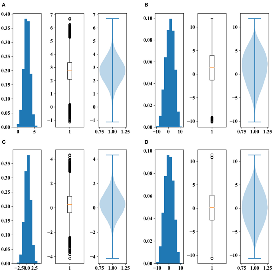
Figure 14. Distributions of the standardized MK statistics, where the sample length is 100 and the slope value is equal to 0.01: (A) PSD = 1, autocorrelation coefficient = 0; (B) PSD = 1, autocorrelation coefficient = 0.9; (C) PSD = 100, autocorrelation coefficient = 0; and (D) PSD = 100, autocorrelation coefficient = 0.9.

By comparing the subfigures of Figure 14, we find that the mean value of the MK statistics decreases with the serial correlation and the PSD value, and the variance in the MK statistics increases with the serial correlation but remains the same as the variation in the PSD. Compared to the variance in the MK statistics, the effect of the mean value is more significant to the rejection rate. The impact of the variance becomes larger when the mean value is small. The effect of the PSD is more pronounced on the mean value of the MK statistics, and the effect of the serial correlation is more obvious on the variance in the MK statistics. Therefore, we conclude that the serial correlation influences the power of the MK test mainly by enlarging the variance in the MK statistics and by decreasing the mean value of the MK statistics. When the mean value of the MK statistics is large, which usually happens with time series that have large slope values and small PSDs, the influence of serial correlation is small and negative. When the mean value of the MK statistics is close to zero, which commonly occurs with time series that have small slope values and large PSDs, the influence of serial correlation on the power of the MK test is large and positive.

Conclusions

For a long time, statistical hypothesis tests have been regarded as “silver bullets” for analysing climate change. However, in a recently published article, the American Statistical Association (ASA) encouraged “Moving to a World Beyond ‘p < 0.05”’ because the significance testing is not as powerful as it seems. Researchers should be more thoughtful when applying these tests (Wasserstein et al., 2019). In this study, we investigated the power of the MK test for detecting monotonic trends in hydrometeorological time series against random terms of different uncertainty levels. The results of Monte Carlo simulation experiments indicate that there is a deterministic relation (Equation 11) between the slope value and the PSD of white noise, which can be used for evaluating the power of the MK test. Based on those equations, the magnitude of the slope beyond which the MK test is effective can be roughly estimated by the length and the variance in the sample. A variable upper limit of the slope value that is associated with the PSD of white noise has been adopted to evaluate the power of the MK test, which is different from the previous studies using a fixed upper limit but seems more accordant with practical situations. When the scope of the slope value is set from 10⁻⁵ to 10⁻¹ × SD, the power of the MK test ranges from ~0.61 to 0.22, corresponding to PSD values equal to 10⁻⁴ and 10⁴, respectively. The way to resist the PSD of white noise for maintaining a specific power is extending the sample length to a required minimum value because the power of the MK test is an increasing function of the sample length. Simulation experiments show that the positive serial correlation existing in the time series will increase the Type I error by increasing the variance in the MK test statistics, and the effects are unconcerned with the variance in the sample. Moreover, the positive serial correlation existing in the time series will decrease the power of the MK test, in other words, increase the probability of Type II error. This influence is mainly from enlarging the variance in the MK statistics and from decreasing the mean value of the MK statistics. By presenting this article, we hope that researchers who use the MK test in their future studies realize that the power of the MK test is not as strong as it seems, especially for limited sample length and large sample variance. To improve the situation, we can slightly increase the significance level, such as from 0.05 to 0.1, or delay the analysis to lengthen the sample time series. For different variables, the required lengths could be very different, which can be much shorter for temperature and humidity time series than for runoff and precipitation time series.

Data Availability Statement

The datasets generated for this study are available on request to the corresponding author.

Author Contributions

FW responses for the concept and design of the work and drafting papers. WS, HY, and GK responses for important revisions to papers. XH responses for approval of final papers to be published. DZ, MR, and GW responses for data collection.

Funding

This research was funded by the National Key R&D Program of China (2017YFC1502706), the National Key R&D Program of China (2018YFC1508003), the Beijing Natural Science Foundation (8181001 and 8184094), the IWHR Research & Development Support Program (JZ0145B022019 and JZ0145B772017), and the National Natural Science Foundation of China (41807286 and 51809281).

Conflict of Interest

The authors declare that the research was conducted in the absence of any commercial or financial relationships that could be construed as a potential conflict of interest.

References

Bai, X., Zeng, J., Chen, K., Li, Z., Zeng, Y., Wen, J., et al. (2019). Parameter optimization of a discrete scattering model by integration of global sensitivity analysis using SMAP active and passive observations. IEEE Trans. Geosci. Remote Sens. 57, 1084–1099. doi: 10.1109/TGRS.2018.2864689

CrossRef Full Text | Google Scholar

Bayazit, M. (2015). Nonstationarity of hydrological records and recent trends in trend analysis: a state-of-the-art review. Environ. Proces. 2, 527–542. doi: 10.1007/s40710-015-0081-7

CrossRef Full Text | Google Scholar

Bayazit, M., and Önöz, B. (2004). Comment on “Applicability of prewhitening to eliminate the influence of serial correlation on the Mann-Kendall test” by Sheng Yue and Chun Yuan Wang. Water Resour. Res. 40:W08801. doi: 10.1029/2002WR001925

CrossRef Full Text | Google Scholar

Bayazit, M., and Önöz, B. (2007). To prewhiten or not to prewhiten in trend analysis? Hydrol. Sci. J. 52, 611–624. doi: 10.1623/hysj.52.4.611

CrossRef Full Text | Google Scholar

Bayley, G. V., and Hammersley, J. M. (1946). The “Effective” number of independent observations in an autocorrelated time series. Suppl. J. R. Statist. Soc. 8, 184–197. doi: 10.2307/2983560

CrossRef Full Text | Google Scholar

Burn, D. H., Hannaford, J., Hodgkins, G. A., Whitfield, P. H., Thorne, R., and Marsh, T. (2012). Reference hydrologic networks II. using reference hydrologic networks to assess climate-driven changes in streamflow. Hydrol. Sci. J. 57, 1580–1593. doi: 10.1080/02626667.2012.728705

CrossRef Full Text | Google Scholar

Chebana, F., Aissia, M. A. B., and Ouarda, T. B. M. J. (2017). Multivariate shift testing for hydrological variables, review, comparison and application. J. Hydrol. 548, 88–103. doi: 10.1016/j.jhydrol.2017.02.033

CrossRef Full Text | Google Scholar

Cong, Z., Zhao, J., Yang, D., and Ni, G. (2010). Understanding the hydrological trends of river basins in China. J. Hydrol. 388, 350–356. doi: 10.1016/j.jhydrol.2010.05.013

CrossRef Full Text | Google Scholar

Cox, D. R., and Stuart, A. (1955). Some quick sign tests for trend in location and dispersion. Biometrika 42, 80–95. doi: 10.1093/biomet/42.1-2.80

CrossRef Full Text | Google Scholar

Dong, J., Crow, W. T., Duan, Z., Wei, L., and Lu, Y. (2019). A double instrumental variable method for geophysical product error estimation. Remote Sens. Environ. 225, 217–228. doi: 10.1016/j.rse.2019.03.003

CrossRef Full Text | Google Scholar

Douglas, E. M., Vogel, R. M., and Kroll, C. N. (2000). Trends in floods and low flows in the United States: impact of spatial correlation. J. Hydrol. 240, 90–105. doi: 10.1016/S0022-1694(00)00336-X

CrossRef Full Text | Google Scholar

Duan, Z., Chen, Q., Chen, C., Liu, J., Gao, H., Song, X., et al. (2018). Spatiotemporal analysis of nonlinear trends in precipitation over Germany during 1951-2013 from multiple observation-based gridded products. Int. J. Climatol. 39, 2120–2135. doi: 10.1002/joc.5939

CrossRef Full Text | Google Scholar

Duan, Z., Tuo, Y., Liu, J., Gao, H., Song, X., Zhang, Z., et al. (2019). Hydrological evaluation of open-access precipitation and air temperature datasets using SWAT in a poorly gauged basin in Ethiopia. J. Hydrol. 569, 612–626. doi: 10.1016/j.jhydrol.2018.12.026

CrossRef Full Text | Google Scholar

Gao, H., Birkel, C., Hrachowitz, M., Tetzlaff, D., Soulsby, C., and Savenije, H. H. G. (2019). A simple topography-driven and calibration-free runoff generation module. Hydrol. Earth Syst. Sci. 23, 787–809. doi: 10.5194/hess-23-787-2019

CrossRef Full Text | Google Scholar

Gao, H., Li, H., Duan, Z., Ren, Z., Meng, X., and Pan, X. (2018). Modelling glacier variation and its impact on water resource in the Urumqi Glacier no. 1 in Central Asia. Sci. Tot. Environ. 644, 1160–1170. doi: 10.1016/j.scitotenv.2018.07.004

PubMed Abstract | CrossRef Full Text | Google Scholar

Hamed, K. H. (2007). Improved finite-sample Hurst exponent estimates using rescaled range analysis. Water Resour. Res. 43, 797–809. doi: 10.1029/2006WR005111

CrossRef Full Text | Google Scholar

Hamed, K. H. (2008). Trend detection in hydrologic data: the Mann–Kendall trend test under the scaling hypothesis. J. Hydrol. 349, 350–363. doi: 10.1016/j.jhydrol.2007.11.009

CrossRef Full Text | Google Scholar

Hamed, K. H. (2009). Enhancing the effectiveness of prewhitening in trend analysis of hydrologic data. J. Hydrol. 368, 143–155. doi: 10.1016/j.jhydrol.2009.01.040

CrossRef Full Text | Google Scholar

Hamed, K. H., and Ramachandra Rao, A. (1998). A modified Mann-Kendall trend test for autocorrelated data. J. Hydrol. 204, 182–196. doi: 10.1016/S0022-1694(97)00125-X

CrossRef Full Text | Google Scholar

Helsel, D., and Hirsch, R. (1992). Statistical Methods in Water Resources. Amsterdam: Elsevier.

Google Scholar

Hipel, K. W., McLeod, A. J., and Weller, R. R. (1988). Data analysis of water quality time series in lake erie1. J. Am. Water Res. Assoc. 24, 533–544. doi: 10.1111/j.1752-1688.1988.tb00903.x

CrossRef Full Text | Google Scholar

Hirsch, R. M. (2011). A perspective on nonstationarity and water management1. J. Am. Water Resour. Assoc. 47, 436–446. doi: 10.1111/j.1752-1688.2011.00539.x

CrossRef Full Text | Google Scholar

Hirsch, R. M., and Slack, J. R. (1984). A nonparametric trend test for seasonal data with serial dependence. Water Resour. Res. 20, 727–732. doi: 10.1029/WR020i006p00727

CrossRef Full Text | Google Scholar

Hirsch, R. M., Slack, J. R., and Smith, R. A. (1982). Techniques of trend analysis for monthly water quality data. Water Resour. Res. 18, 107–121. doi: 10.1029/WR018i001p00107

CrossRef Full Text | Google Scholar

Kan, G., Li, J., Zhang, X., Ding, L., He, X., Liang, K., et al. (2017a). A new hybrid data-driven model for event-based rainfall–runoff simulation. Neural Comput. Appl. 28, 2519–2534. doi: 10.1007/s00521-016-2200-4

CrossRef Full Text | Google Scholar

Kan, G., Tang, G., Yang, Y., Hong, Y., Li, J., Ding, L., et al. (2017b). An improved coupled routing and excess storage (CREST) distributed hydrological model and its verification in Ganjiang River Basin, China. Water 9:904. doi: 10.3390/w9110904

CrossRef Full Text | Google Scholar

Kan, G., Zhang, M., Liang, K., Wang, H., Jiang, Y., Li, J., et al. (2018). Improving water quantity simulation & forecasting to solve the energy-water-food nexus issue by using heterogeneous computing accelerated global optimization method. Appl. Energy 210, 420–433. doi: 10.1016/j.apenergy.2016.08.017

CrossRef Full Text | Google Scholar

Kendall, M. G. (1975). Rank Correlation Methods. New York, NY: Oxford University Press.

Google Scholar

Kulkarni, A., and Von Storch, H. (1995). Monte carlo experiments on the effect of serial correlation on the Mann-Kendall test of trend. Meteorol. Zeitschrift 4, 82–85. doi: 10.1127/metz/4/1992/82

CrossRef Full Text | Google Scholar

Lettenmaier, D., Wood, E., and Wallis, J. (1994). Hydro-climatological trends in the continental United States, 1948-88. J. Climate. 7, 586–607. doi: 10.1175/1520-0442(1994)007<0586:HCTITC>2.0.CO;2

CrossRef Full Text | Google Scholar

Lettenmaier, D. P. (1976). Detection of trends in water quality data from records with dependent observations. Water Resour. Res. 12, 1037–1046. doi: 10.1029/WR012i005p01037

CrossRef Full Text | Google Scholar

Lettenmaier, D. P. (1988). Multi variate nonparametric tests for trend in water quality. Water Resour. Bullet. 24, 505–512. doi: 10.1111/j.1752-1688.1988.tb00900.x

CrossRef Full Text | Google Scholar

Mann, H. B. (1945). Nonparametric tests against trend. Econometrica 13, 245–259. doi: 10.2307/1907187

CrossRef Full Text | Google Scholar

Milly, P. C., Betancourt, J., Falkenmark, M., Hirsch, R. M., Kundzewicz, Z. W., Lettenmaier, D. P., et al. (2008). Stationarity is dead: whither water management? Science 319, 573–574. doi: 10.1126/science.1151915

PubMed Abstract | CrossRef Full Text | Google Scholar

Milly, P. C. D., Betancourt, J., Falkenmark, M., Hirsch, R. M., Kundzewicz, Z. W., Lettenmaier, D. P., et al. (2015). On critiques of “Stationarity is dead: whither water management?”. Water Resour. Res. 51, 7785–7789. doi: 10.1002/2015WR017408

CrossRef Full Text | Google Scholar

Montanari, A., and Koutsoyiannis, D. (2014). Modeling and mitigating natural hazards: stationarity is immortal! Water Resour. Res. 50, 9748–9756. doi: 10.1002/2014W.R.016092

CrossRef Full Text | Google Scholar

Önöz, B., and Bayazit, M. (2003). The power of statistical tests for trend detection. Turkish J. Eng. Environ. Sci. 27, 247–251. doi: 10.3906/sag-1205-120

CrossRef Full Text | Google Scholar

Rehan, B. M., and Hall, J. W. (2014). “Flood risk management decision analysis With finite historical records and highly variable climate effects,” Vulnerability, Uncertainty, and Risk, 2867–2879. doi: 10.1061/9780784413609.289

CrossRef Full Text | Google Scholar

Sang, Y.-F., Wang, Z., and Liu, C. (2014). Comparison of the MK test and EMD method for trend identification in hydrological time series. J. Hydrol. 510, 293–298. doi: 10.1016/j.jhydrol.2013.12.039

CrossRef Full Text | Google Scholar

Sen, P. K. (1968). Estimates of the regression coefficient based on Kendall's Tau. J. Am. Statist. Assoc. 63, 1379–1389. doi: 10.1080/01621459.1968.10480934

CrossRef Full Text | Google Scholar

Serinaldi, F., and Kilsby, C. G. (2016). The importance of prewhitening in change point analysis under persistence. Stochastic Environ. Res. Risk Assess. 30, 763–777. doi: 10.1007/s00477-015-1041-5

CrossRef Full Text | Google Scholar

Serinaldi, F., Kilsby, C. G., and Lombardo, F. (2018). Untenable nonstationarity: an assessment of the fitness for purpose of trend tests in hydrology. Adv. Water Resour. 111, 132–155. doi: 10.1016/j.advwatres.2017.10.015

CrossRef Full Text | Google Scholar

Shao, W., Bogaard, T., Bakker, M., and Berti, M. (2016). The influence of preferential flow on pressure propagation and landslide triggering of the Rocca Pitigliana landslide. J. Hydrol. 543, 360–372. doi: 10.1016/j.jhydrol.2016.10.015

CrossRef Full Text | Google Scholar

Shao, W., Coenders-Gerrits, M., Judge, J., Zeng, Y., and Su, Y. (2018). The impact of non-isothermal soil moisture transport on evaporation fluxes in a maize cropland. J. Hydrol. 561, 833–847. doi: 10.1016/j.jhydrol.2018.04.033

CrossRef Full Text | Google Scholar

Theil, H. (1950). “A rank invariant method of linear and polynomial regression analysis,” in Proceedings of the Royal Netherlands Academy of Sciences, Series A Mathematical Sciences, Vol. 53, Part I: 386-392, Part II: 521-525, Part III: 1397-1412 (Amsterdam).

Google Scholar

Tian, Y., Xu, Y.-P., and Wang, G. (2018a). Agricultural drought prediction using climate indices based on support vector regression in Xiangjiang River basin. Sci. Tot. Environ. 622–623, 710–720. doi: 10.1016/j.scitotenv.2017.12.025

PubMed Abstract | CrossRef Full Text | Google Scholar

Tian, Y., Zhang, K., Xu, Y.-P., Gao, X., and Wang, J. (2018b). Evaluation of potential evapotranspiration based on CMADS reanalysis dataset over China. Water 10:1126. doi: 10.3390/w10091126

CrossRef Full Text | Google Scholar

Vogel, R. M., Rosner, A., and Kirshen, P. H. (2013). Brief communication: likelihood of societal preparedness for global change: trend detection. Nat. Hazards Earth Syst. Sci. 13, 1773–1778. doi: 10.5194/nhess-13-1773-2013

CrossRef Full Text | Google Scholar

Von Storch, H., and Navarra, A. (1995). Analysis of Climate Variability Applications of Statistical Techniques. Berlin: Springer-Verlag. 1–26

Google Scholar

Wang, K., Liu, X., Tian, W., Li, Y., Liang, K., Liu, C., et al. (2019). Pan coefficient sensitivity to environment variables across China. J. Hydrol. 572, 582–591. doi: 10.1016/j.jhydrol.2019.03.039

CrossRef Full Text | Google Scholar

Wang, K., Yang, X., Liu, X., and Liu, C. (2017). A simple analytical infiltration model for short-duration rainfall. J. Hydrol. 555, 141–154. doi: 10.1016/j.jhydrol.2017.09.049

CrossRef Full Text | Google Scholar

Wang, S., Zuo, H., Yin, Y., Hu, C., Yin, J., Ma, X., et al. (2019). Interpreting rainfall anomalies using rainfall's nonnegative nature. Geophys. Res. Lett. 46, 426–434. doi: 10.1029/2018GL081190

CrossRef Full Text | Google Scholar

Wasserstein, R. L., Schirm, A. L., and Lazar, N. A. (2019). Moving to a world beyond “p <0.05”. Am. Statist. 73, 1–19. doi: 10.1080/00031305.2019.1583913

CrossRef Full Text | Google Scholar

Yevjevich, V. (1974). Determinism and stochasticity in hydrology. J. Hydrol. 22, 225–238. doi: 10.1016/0022-1694(74)90078-X

CrossRef Full Text | Google Scholar

Yu, W., Li, Y., Cao, Y., and Schillerberg, T. (2019). Drought assessment using GRACE terrestrial water storage deficit in Mongolia from 2002 to 2017. Water 11:1301. doi: 10.3390/w11061301

CrossRef Full Text | Google Scholar

Yue, S., and Pilon, P. (2004). A comparison of the power of the t test, Mann-Kendall and bootstrap tests for trend detection / Une comparaison de la puissance des tests t de Student, de Mann-Kendall et du bootstrap pour la détection de tendance. Hydrol. Sci. J. 49, 21–37. doi: 10.1623/hysj.49.1.21.53996

CrossRef Full Text | Google Scholar

Yue, S., Pilon, P., and Cavadias, G. (2002a). Power of the Mann–Kendall and Spearman's rho tests for detecting monotonic trends in hydrological series. J. Hydrol. 259, 254–271. doi: 10.1016/S0022-1694(01)00594-7

CrossRef Full Text | Google Scholar

Yue, S., Pilon, P., Phinney, B., and Cavadias, G. (2002b). The influence of autocorrelation on the ability to detect trend in hydrological series. Hydrol; Process. 16, 1807–1829. doi: 10.1002/hyp.1095

CrossRef Full Text | Google Scholar

Yue, S., Pilon, P., and Phinney, B. O. B. (2003). Canadian streamflow trend detection: impacts of serial and cross-correlation. Hydrol. Sci. J. 48, 51–63. doi: 10.1623/hysj.48.1.51.43478

CrossRef Full Text | Google Scholar

Yue, S., and Wang, C. (2004). The Mann-Kendall test modified by effective sample size to detect trend in serially correlated hydrological series. Water Resour. Manage. 18, 201–218. doi: 10.1023/B:WARM.0000043140.61082.60

CrossRef Full Text | Google Scholar

Yue, S., and Wang, C. Y. (2002). Applicability of prewhitening to eliminate the influence of serial correlation on the Mann-Kendall test. Water Resour. Res. 38, 4-1-4-7. doi: 10.1029/2001WR000861

CrossRef Full Text | Google Scholar

Zhang, X., and Zwiers, F. W. (2004). Comment on “Applicability of prewhitening to eliminate the influence of serial correlation on the Mann-Kendall test” by Sheng Yue and Chun Yuan Wang. Water Resour. Res. 40:W03805. doi: 10.1029/2003WR002073

CrossRef Full Text | Google Scholar

Zhu, Y., Liu, Y., Ma, X., Ren, L., and Singh, P. V. (2018). Drought analysis in the Yellow River Basin based on a short-scalar palmer drought severity index. Water 10:1526. doi: 10.3390/w10111526

CrossRef Full Text | Google Scholar