- 1Institute of Coastal Research, Helmholtz-Zentrum Geesthacht, Geesthacht, Germany
- 2Max Planck Institute for Meteorology, Hamburg, Germany
Regional coupled system models require a high-resolution discharge component to couple their atmosphere/land components to the ocean component and to adequately resolve smaller catchments and the day-to-day variability of discharge. As the currently coupled discharge models usually do not fulfill this requirement, we improved a well-established discharge model, the Hydrological Discharge (HD) model, to be globally applicable at 5 Min. resolution. As the first coupled high-resolution discharge simulations are planned over Europe and the Baltic Sea catchment, we focus on the respective regions in the present study. As no river specific parameter adjustments were conducted and since the HD model parameters depend on globally available gridded characteristics, the model is, in principle, applicable for climate change studies and over ungauged catchments. For the validation of the 5 Min. HD (HD5) model, we force it with prescribed fields of surface and subsurface runoff. As no large-scale observations of these variables exist, they need to be calculated by a land surface scheme or hydrology model using observed or re-analyzed meteorological data. In order to pay regard to uncertainties introduced by these calculations, three different methods and datasets were used to derive the required fields of surface and subsurface runoff for the forcing of the HD5 model. However, the evaluation of the model performance itself is hampered by biases in these fields as they impose an upper limit on the accuracy of simulated discharge. 10-years simulations (2000–2009) show that for many European rivers, where daily discharge observations were available for comparison, the HD5 model captures the main discharge characteristics reasonably well. Deficiencies of the simulated discharge could often be traced back to deficits in the various forcing datasets. As direct anthropogenic impact on the discharge, such as by regulation or dams, is not regarded in the HD model, those effects can generally not be simulated. Thus, discharges for many heavily regulated rivers in Scandinavia or for the rivers Volga and Don are not well represented by the model. The comparison of the three sets of simulated discharges indicates that the HD5 model is suitable to evaluate the terrestrial hydrological cycle of climate models or land surface models, especially with regard to the separation of throughfall (rain or snow melt) into surface and subsurface runoff.
Introduction
The hydrological cycle is crucially important to life on Earth since water is essential nourishment for all organisms. Consequently, the importance of the hydrological cycle is highlighted by the Global Energy and Water Cycle Experiment (GEWEX; e.g., Sorooshian et al., 2005), which is now in its third phase (2013–20221). The implications of changes in the hydrological cycle induced by climate change may affect the society more than any other changes, e.g., with regard to flood risks, water availability and water quality. For example, large irrigation activities in many parts of Middle Asia led to man-made climate change in the Aral Sea region that were caused by the lake’s catastrophic desiccation within the last five decades (Breckle and Geldyeva, 2012). This had severe consequences for the societies living in this area. Another example is the prominent drought period in the Sahel that began at the end of the 1960s and ended in the mid-1980s (Anyamba and Tucker, 2005). This caused a noticeable decline of per capita food production and food self-sufficiency ratios in the Sahel (Epule et al., 2014).
Discharge (or river runoff) is an important component of the global water cycle and comprises about one third of the precipitation over land areas. It closes the water cycle between land and ocean. On the one hand, the freshwater inflow affects the thermohaline circulation, especially in regions where deep convection occurs (Hordoir et al., 2008). For example, an increased freshwater anomaly may cause a weakening of the meridional overturning in the Northern Atlantic (Marzeion et al., 2007). An important source of stratification in the North−Western European Shelf is the outflow from the Baltic Sea (Hordoir and Meier, 2010) that is mainly induced by river runoff into and net precipitation over the Baltic Sea. Decadal variations in Baltic Sea salinity are caused largely by the accumulated runoff to the Baltic Sea (Väli et al., 2013). In addition, the thermohaline circulation of the Baltic Sea is also influenced by inflows of highly saline water from the North Sea that itself may be strongly impacted by uncertainties in precipitation and/or river runoff (Lehmann and Hinrichsen, 2000).
On the other hand, river discharge and the associated nutrient loads are important factors that influence the functioning of the marine ecosystem. Lateral inflows from land, carrying fresh, nutrient-rich water determine coastal physical conditions and nutrient concentration and, hence, dominantly influence primary production in the system. Since this forms the basis of the trophic food web, it impacts the variability of the whole ecosystem (Daewel and Schrum, 2017). This becomes even more relevant in systems like the Baltic Sea, which is almost decoupled from the open ocean and land-borne nutrients play a major role for determining ecosystem productivity (Thurow, 1997; Österblom et al., 2007). With respect to global biogeochemical cycles, a proper description of the transport of, e.g., nitrogen, phosphorus, carbon, and silicon, into the ocean requires a very detailed representation of stream characteristics (such as flow paths, lakes, ponds, reservoirs, wetlands, and floodplains) because the smallest water bodies may exhibit large parts of the retention on land (Bouwman et al., 2013).
In climate change studies, runoff is generated differently in hydrological and climate modeling communities. In hydrology, global hydrology models (GHMs) or local/regional hydrological models (HMs) are used that are forced with climate model input. This method has two major advantages. First, the GHMS and HMs are specific impact models focusing on hydrology, and, hence, hydrology is not just one of many processes such as it is in a climate model where the main purpose is to simulate the climate. Second, it is well known that general circulation models (GCMs) and regional climate models (RCMs) suffer from substantial biases, especially with regard to precipitation and the hydrological cycle (Flato et al., 2013; Kotlarski et al., 2014). When using GHMs or HMs, climate model input can still be bias-corrected before these data are fed into the hydrology model. Local and regional HMs are often calibrated. On the one hand, this leads to more accurate discharge simulations for current climate. On the other hand, the calibration may obscure deficiencies in process representations that may lead to erroneous behavior in ungauged catchments or different climates under global warming conditions. On the downside of the HM application is that no feedbacks to the atmosphere are considered, and the simulated hydrology may be inconsistent with climate model forcing. Using different models changes the uncertainty of the results (Hagemann et al., 2013). This is especially important when using a model chain comprising bias corrected GCM data fed into GHMs as being applied within the European Union (EU) project WATer and global Change (WATCH2; see, e.g., Harding et al., 2011) and the Inter-Sectoral Impact Model Intercomparison Project (ISIMIP; Warszawski et al., 2014).
In climate modeling, runoff is generated within the land surface schemes of global or regional climate models. Thus, the simulated runoff and other hydrological variables are consistent with the climate variables and hydrology – atmosphere feedbacks are regarded. A disadvantage is that potentially large biases exists due to climate model biases, especially in precipitation (see above). This approach is used for coupled system model studies, where interactions between the different compartments of the Earth system shall be considered. In a coupled Earth system model, the discharge is the interface between the land surface hydrology and the ocean, and thus an integral part of the coupled system.
For global applications of a discharge model within a fully coupled GCM or an Earth System Model (ESM), a grid resolution of 0.5° is usually sufficient. The same applies for regional applications of coupled system models where the main objective is an adequate representation of the mean monthly discharge of large rivers. If research and applications focus on the representation of daily discharge, consider smaller catchments or investigate the transport of biogeochemical compounds on the regional scale, higher resolutions are required for the appropriate simulation of discharge. Zhao et al. (2017) demonstrated the importance of the routing scheme (i.e., the discharge model) to simulate peak discharges. Their routing model did not only account for floodplain storage and backwater effects that are not represented in most GHMs, but also was using a higher resolution (0.25°) than the nine GHMs (0.5°) from which the forcing data were taken. While most of the GHMs use a 0.5° resolution, some of them are available at higher resolutions, e.g., LISFLOOD at 0.1° (Van Der Knijff et al., 2010), PCR-GLOBWB at 0.08° (López López et al., 2016) and WaterGap3 at 5 Min. (Flörke et al., 2013). Moreover, several large-scale regional HMs exist, such as E-Hype with a median catchment size of 215 km2 (Donnelly et al., 2016; Lindström et al., 2010), LISFLOOD at 5 km and mHM at 1–24 km (Samaniego et al., 2010) for Europe, and MODCOU at 1–8 km over France (Decharme et al., 2013). Bierkens et al. (2015) summarized ongoing and planned activities in large-scale high-resolution hydrological modeling.
In addition to traditional RCMs, regional coupled system models (RCSM) have been recently developed to conduct climate change studies at high spatial and temporal resolutions. These models require a high-resolution discharge component to couple their atmosphere/land components to the ocean component and to adequately resolve smaller catchments and the day-to-day variability of discharge. The current discharge models applied in coupled (or Earth system) models for global or regional climate simulations usually do not fulfill this requirement. In ESMs, discharge (or routing) models are frequently part of the coupled system (often as part of the land surface scheme) but their spatial resolution is usually 0.5° (Roeckner et al., 2003; Guimberteau et al., 2012) or coarser (Best et al., 2011; Lawrence et al., 2011; Milly et al., 2014). For RCSMs, a few setups exists where a discharge model is included, but its resolution is rarely higher than 0.5°. Examples comprise the HD model (Hagemann and Dümenil, 1998) at 0.5° (Elizalde, 2011; Sein et al., 2015; Sitz et al., 2017), TRIP (Oki and Sud, 1998) at 0.5° (Dell’Aquila et al., 2012; Sevault et al., 2014) and LARSIM (Bremicker, 2000) at 1/6° over Northern Europe (Lorenz and Jacob, 2014). Several studies exists where a RCM was coupled to a very-high resolution regional HM but currently these studies cover only short periods or relatively small catchments/areas (e.g., Mauser and Bach, 2009; Larsen et al., 2014; Shrestha et al., 2014; Senatore et al., 2015). Over Korea, the discharge model TRIP has been coupled to a RCM at 0.5°, 0.25°, and 0.125° in preparation of future RCMS studies (Lee et al., 2015). To our knowledge, none of the HMs used in the studies listed above has been used in a fully coupled RCSM setup that can be applied for climate time scales and large-scale areas.
At the Helmholtz-Zentrum Geesthacht, RCSM simulations are planned with GCOAST (Geesthacht Coupled cOAstal model SysTem) over Europe and the Baltic Sea (Ho-Hagemann et al., submitted). Consequently, to prepare high-resolution discharge simulations over these regions within GCOAST, we further developed a well-established discharge model, the Hydrological Discharge (HD) model (Hagemann and Dümenil, 1998), to be globally applicable at 5 Min. resolution. Here, we chose to follow the climate modeling approach (see above) to calculate discharge, as the simulated discharge should be consistent with the climate model forcing. For the planned application within a RCSM, we aim at simulating river discharge with a realistic daily variability and capturing the timing and magnitude of the main peaks and low flow periods on the daily time scale. The representation of minor short-term daily fluctuations is not required, as this is neither expected to be obtained from RCSM simulations nor from using coarse resolution forcing datasets as utilized for the evaluation of the model results in the present study. This study shows first results in comparison with available observations over Europe and the Baltic Sea catchment. The HD model, data and evaluation metrics are described in section “Data and Methods.” In section “Results,” the forcing data and the discharge simulations are evaluated and discussed, followed by section “Summary and Conclusion” where a summary and conclusions are provided.
Data and Methods
With regard to the lateral flow of water at the land surface, the term runoff is often used, which commonly leads to some communication problems. Sometimes it refers to the water from rain and snowmelt that is not infiltrated into the soil (surface runoff), to the whole amount of water that may be transported laterally at a certain location (total runoff), or to the amount of water that is already laterally transported as discharge by rivers (river runoff). In the long-term annual mean, total runoff equals discharge within a catchment, and in this case, runoff is equivalent to precipitation minus evaporation averaged over the catchment. To avoid these communication problems the clear specification of the term runoff is generally recommended and subsequently used in the present study. Here, runoff refers to the total runoff and comprises surface runoff and drainage from the soil (or subsurface runoff). The first represents water amounts that may flow laterally off at the surface or the near-surface layers of the soil, while the latter designates the respective water amounts in the deeper layers of the soil.
The HD Model
The HD model (Hagemann and Dümenil, 1998; Hagemann and Dümenil Gates, 2001) is used in this study for the calculation of river runoff. The HD model has already been used for many years in the global ESM of the Max Planck Institute for Meteorology (MPI-M), MPI-ESM (Giorgetta et al., 2013), and its predecessor ECHAM5/MPIOM (Roeckner et al., 2003; Jungclaus et al., 2006). Recently, it was also included in the regional ESMs ROM (Sein et al., 2015) and RegCM-ES (Sitz et al., 2017) as well as the regional climate model REMO-MPIOM (Elizalde, 2011). Furthermore, the HD model is currently implemented into the RCSMGCOAST of the Helmholtz-Zentrum Geesthacht. The HD model was designed to run on a fixed global regular grid of 0.5° horizontal resolution, and it uses a pre-computed river channel network to simulate the horizontal transport of water within model watersheds. Originally, the HD model used a daily time step, but some refinements made during the MPI-ESM development allow sub-daily time steps, e.g., hourly.
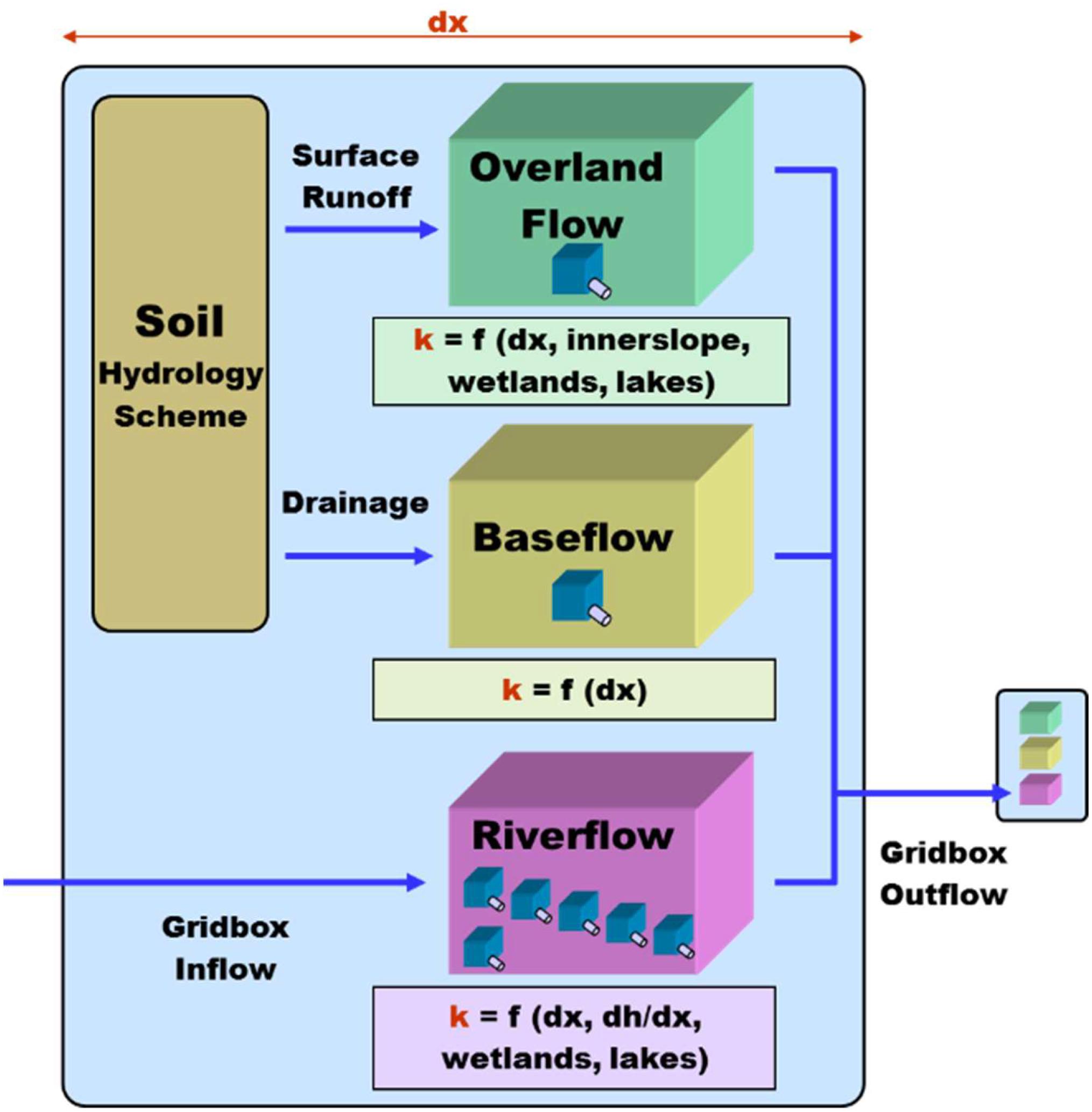
Figure 1 shows the structure of the HD model. It separates the lateral water flow into the three flow processes of overland flow, baseflow, and riverflow. Overland flow and baseflow represent the fast and slow lateral flow processes within a grid box, while riverflow represents the lateral flow between grid boxes. Overland flow and baseflow are both computed using a single linear reservoir. The first uses surface runoff as input, while the latter is fed by drainage from the soil. Riverflow receives the inflow from other grid boxes as input and it is simulated by a cascade of five equal linear reservoirs. The sum of the three flow processes is equal to the total outflow from a grid box. The model parameters are functions of the topography gradient between grid boxes, the slope within a grid box, the grid box length, the lake area, and the wetland fraction of a particular grid box. The model input fields of surface runoff and drainage resulting from the various climate or land surface model resolutions are interpolated to the HD grid before being fed into the HD model.
Model Improvements
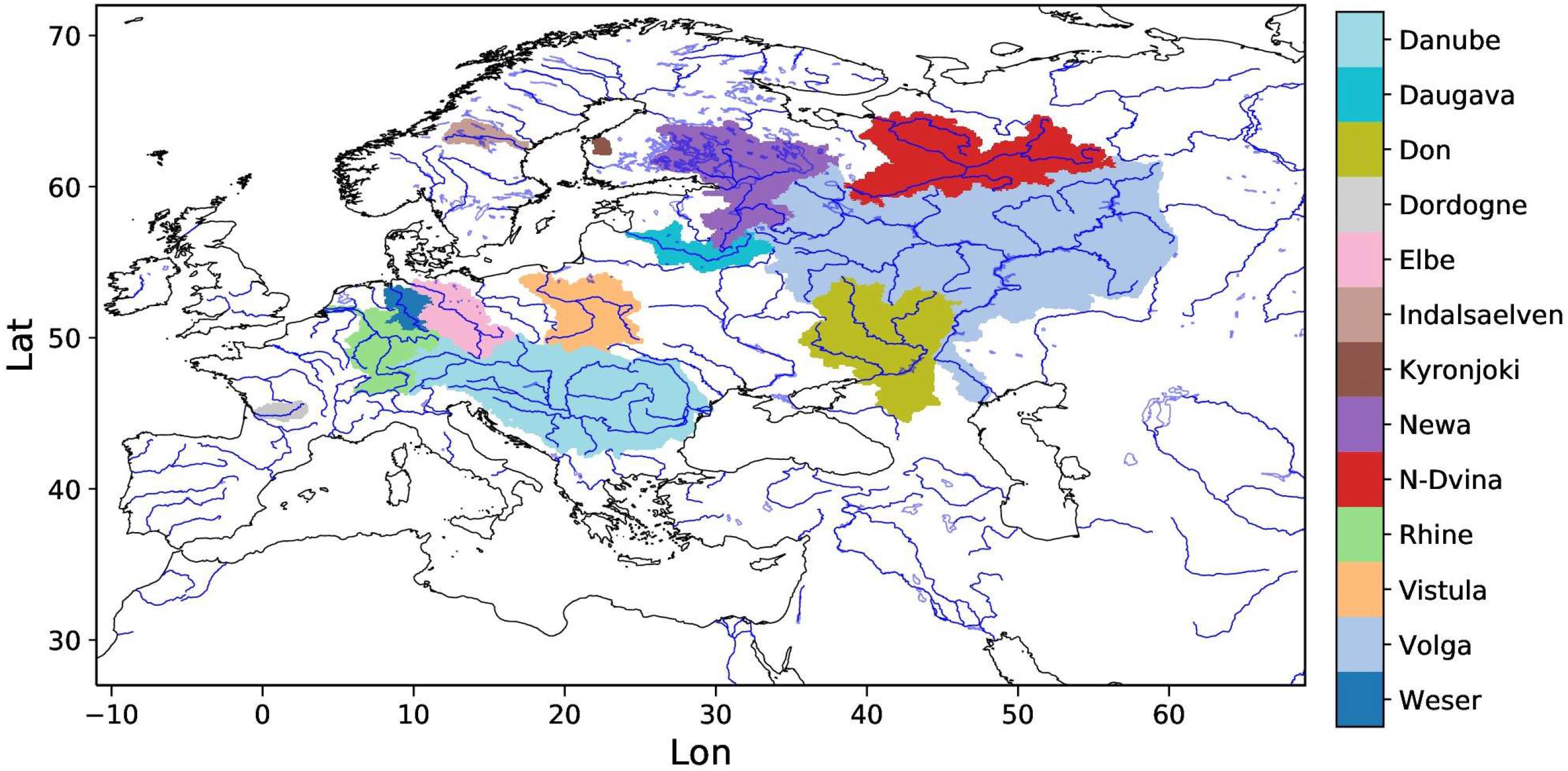
The HD model has been adapted to run on a regular grid of 5 Min. horizontal resolution, which corresponds to an average grid box size of 8–9 km. It can be forced with daily or sub-daily time series of surface runoff and drainage using a time step that equals the forcing time step. In the present study, the model time step was set to the respective forcing time step (see section “Forcing Data and Experimental Setup”). However, as the minimum travel time through a grid box is limited by the time step chosen, an internal time step of 0.5 h is used for riverflow. For the initial development and application of the 5 Min. HD version (HD5), a regional domain over Europe was chosen that covers the land areas between −1°W to 69°E and 27°N to 72°N. The domain is shown in Figure 2 together with the catchments areas for selected rivers that are specifically mentioned in the manuscript. River directions and digital elevation data were provided by Bernhard Lehner (pers. comm., 2014) and were derived from the HydroSHEDS (Lehner et al., 2006) database and from the Hydro1K dataset for areas north of 60°N3. We compared the HD5 catchment areas with literature values for the whole catchment and with station values for the station-related catchments. In general, we found a good agreement with the observed areas. Larger deviations between gridded and observed areas occur only for a few rivers that are mainly located north of 60°N, i.e., in the Hydro1K part of the HD5 grid. Lake fractions are taken from the European Space Agency (ESA) Land Cover Climate Change Initiative (LC_CCI) for epoch 2010 (version 2.0.7; available at4) and wetland fractions from the LSP2 (Land Surface Parameter vs. 2) dataset (Hagemann, 2002). To adapt the HD model parameters used at 0.5° resolution to the higher resolution, global scaling factors were applied to the reservoir retention coefficients of overland flow and base flow. These two factors are global constants and were applied in every HD model grid box. Thus, as for the operational HD model at 0.5° resolution, no river specific parameter adjustments were conducted. Since the HD model parameters depend on globally available grid box characteristics, it is, in principle, applicable for climate change studies and over ungauged catchments, i.e., river basins where no daily discharges are available at a downstream station. Here, we imply that if the HD5 model yields satisfactory simulated discharges for many rivers without river and time period specific calibration, then we can be confident that the model is likely to also provide reasonable discharge in climate change studies and over ungauged catchments where an evaluation is not possible.
Forcing Data and Experimental Setup
As mentioned in section “Introduction,” it is well known that climate models suffer from substantial biases, especially with regard to precipitation and the hydrological cycle. In order to avoid uncertainties introduced by model biases of the atmospheric component of a RCSM, the HD5 model was driven by pre-generated fields of surface and subsurface runoff. As no large-scale observations of these variables exist, they need to be calculated by a land surface scheme or hydrology model using observed or re-analyzed meteorological data. Figure 3 summarizes the main steps of generating simulated discharges with HD model in stand-alone mode and conducting their evaluation. These steps comprise three parts:
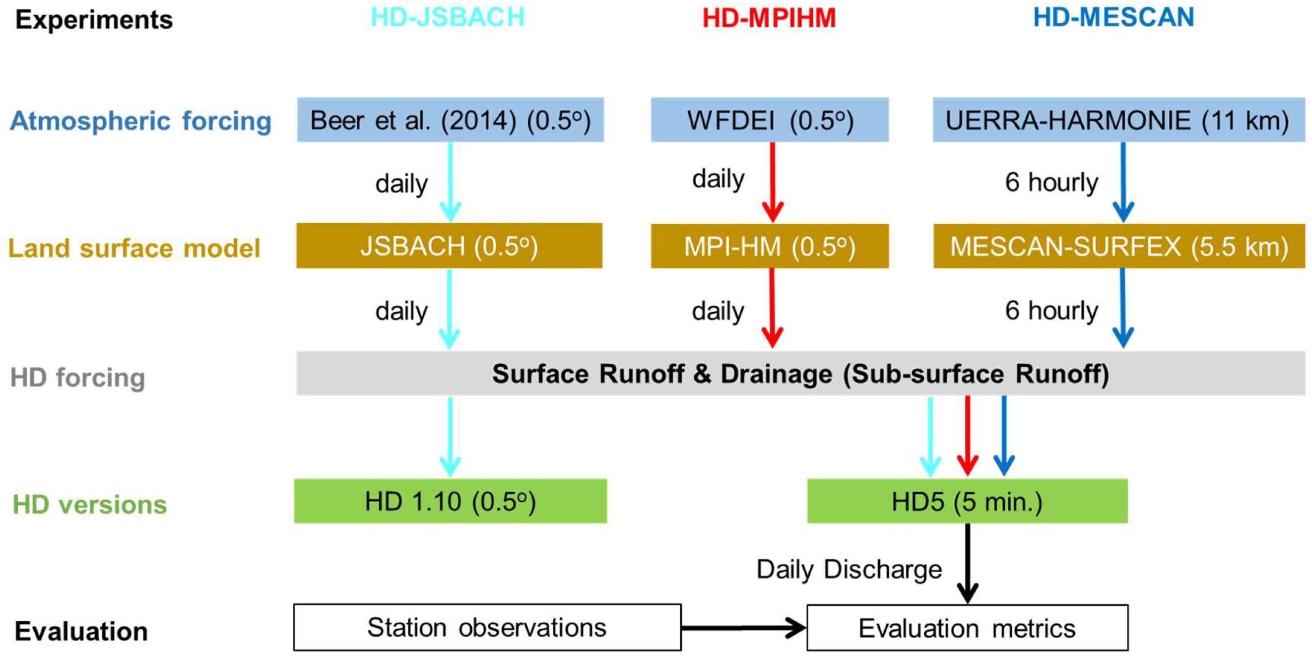
Figure 3. Flowchart showing the main steps of generating simulated discharges with the HD model and conducting their evaluation in the present study.
1. Preparation of HD model forcing: Choose an atmospheric forcing dataset and use a land surface (or hydrology) model to generate the forcing for the HD model,
2. Run the HD model: Interpolate the forcing data of surface runoff and drainage to the HD model grid and simulate daily discharges with the HD model,
3. Evaluation of results: Compare simulated and observed discharges at station location and calculate various evaluation metrics.
Note that in coupled HD model applications, part 1 is replaced by direct input from the respective RCM or GCM. In order to pay regard to uncertainties introduced by the inputs generated in part 1, three different methods and datasets were used to derive the required fields of surface and subsurface runoff for the forcing of the HD5 model. Table 1 provides an overview on these three forcing datasets and their characteristics.
HD5-JSBACH
In order to generate daily input fields of surface runoff and drainage, the land surface scheme JSBACH (vs. 3 + frozen soil physics; Ekici et al., 2014) was forced globally at 0.5° with daily atmospheric forcing data based on the Interim Re-Analysis of the European Center for Medium-Range Weather Forecast (ERA-Interim; Dee et al., 2011). These forcing data are bias-corrected (see Beer et al., 2014) toward the so-called WATCH forcing data (WFD; Weedon et al., 2011) that have been generated in the EU project WATCH. For our study, we spatially interpolated the surface runoff and drainage data to the European 5-Min. domain using conservative remapping and fed into the HD5 model. The simulation period is 1979–2009. This forcing was also used for an analogous simulation with the HD model at 0.5° resolution. This 0.5° simulation is denoted with HD 1.10 in the following.
HD5-MPIHM
The MPI-M hydrology model MPI-HM (Stacke and Hagemann, 2012) was driven by daily WATCH forcing data based on ERA-Interim (WFDEI; Weedon et al., 2014) from 1979–2009 to generate daily input fields of surface runoff and drainage. MPI-HM is a GHM operating at a spatial resolution of 0.5°. It has contributed to the WATCH Water Model Intercomparison Project (WaterMIP; Haddeland et al., 2011) and ISIMIP (Warszawski et al., 2014).
HD5-MESCAN
Six hourly data of surface runoff and drainage (variable name: percolation) were retrieved from the MESCAN-SURFEX regional surface reanalysis (Bazile et al., 2017) created in the EU project UERRA (Uncertainties in Ensembles of Regional ReAnalysis5). SURFEX (Masson et al., 2013) is a land surface platform that was driven by atmospheric forcing at 5.5 km. The forcing comprises 24 h-precipitation, near-surface temperature and relative humidity analyzed by the MESCAN surface analysis system as well as radiative fluxes and wind downscaled at 5.5 km from the 3DVar re-analysis conducted with the HARMONIE system at 11 km (Ridal et al., 2017). The latter has been generated using 6-hourly fields of the ERA-Interim reanalysis as boundary conditions and covers a domain comprising Europe and parts of the Atlantic, which is similar to the European domain of the Coordinated Downscaling Experiment (CORDEX) at 11 km.
Observed Discharge Data
Given the resolution of the HD5 model, an adequate simulation of discharge is not expected for small catchments. Therefore, we only considered rivers with catchment areas around 3000 km2 or larger. Most of the daily discharge data used in this study were provided by the GRDC (Global Runoff Data Center, 56068 Koblenz, Germany). Further data were obtained from various sources such as: Banque Hydro (France), Bundesanstalt für Gewässerkunde Koblenz (Germany), Office of Public Works (Ireland), Norwegian Water and Energy Directorate, Institute of Meteorology and Water Management (Poland), Sistema Nacional de Informação (Portugal), R-ArctivNET (Onega river), Sistema Integrado de Información del Agua (Spain), National River Flow Archive (United Kingdom), and various regional hydrological offices in Italy (Abruzzo, Emilia Romagna, Latio, Puglia, Toscana, Veneto). For each river, the most downstream river gauge was considered for which daily discharge data were available, i.e., from that measurement station, which is closest to the river mouth.
Evaluation Metrics
The discharge evaluation of the HD5 simulations was conducted for those grid boxes that correspond to the station locations within the river network of the respective discharge observations. All evaluation metrics were calculated using simulated and observed time series of daily discharge for the period 2000–2009.
Standard Deviation
The standard deviation σx of a time series xi with n values and the arithmetic mean μx is defined as
Note that we use the standard deviation of a sample (division by n-1), and not the one for the population (division by n).
Coefficient of Variation
The coefficient of variation CVx is defined as the ratio of the standard deviation σx to the mean μx of a time series xi. It shows the extent of variability in relation to the temporal mean.
Pearson Correlation Coefficient
The correlation of two time series xi and yi is expressed by the correlation coefficient rcor of the Pearson product-moment correlation. Alternative names of rcor are Bravais-Pearson correlation, Pearson correlation or just correlation coefficient.
Kling Gupta Efficiency
The Kling Gupta efficiency (KGE) developed by Gupta et al. (2009) is used to measure the agreement between simulated and observed discharge. It provides diagnostically interesting insights into the model performance due to its decomposition of the mean squared model error into correlation, variability and bias terms. This facilitates the analysis of the relative importance of these different components, which is frequently used to evaluate hydrological simulations. Here, we used a revised version of this index (Kling et al., 2012) to ensure that the bias and the variability ratio are not cross-correlated:
with c1 = rcor−1, ,
The computation of KGE comprises three main components:
1. The Pearson correlation coefficient rcor, with an ideal value of one.
2. The variability ratio that is computed by using the coefficients of variation (Kling et al., 2012) of simulated and observed data, with an ideal value of one. Note that in the original method, the ratio of the standard deviations was used (Gupta et al., 2009).
3. The ratio between the means of the simulated values μsim and the observed values μobs, with an ideal value of one. Note that c3 corresponds to the bias of the simulated values.
The Kling-Gupta efficiencies range from negative infinity to one. Essentially, the closer to one, the more accurate the model is. For a full discussion of the KGE-statistic and its advantages over the Nash–Sutcliffe efficiency (Nash and Sutcliffe, 1970) or the mean squared error, see Gupta et al. (2009).
Lag
The lag between two time series describes the temporal discrepancy between the centers of gravity between both time series. The cross correlation or lag correlation coefficient rτ of two time series, which are shifted to each other by τ time steps, is defined as:
The lag L between these two time series is the value of τ where rτ reaches its maximum. For τ = 0 the cross correlation coefficient corresponds to the Pearson correlation coefficient.
Root-Mean-Square-Error (RSME)
The root-mean-square error (RMSE) is a common measure of the differences between simulated (xi) and observed (yi) time series. It is defined as
In the present study, we used the normalized RMSE that facilitates the comparison between datasets or models with different scales, where the RMSE is divided by the range (defined as the maximum value minus the minimum value) of the observed data.
Results
First, a short evaluation of the forcing datasets is provided in this section, and then the impact of a higher spatial resolution on the simulated discharge is addressed. The results of the 5 Min. simulations are evaluated in section “Evaluation of 5 Min. Simulations,” which is followed by a discussion of the results. Note that since we do not have perfect forcing data of surface and subsurface runoff, the evaluation of simulated discharge is not straight forward, as deficiencies may be caused by shortcomings in the HD5 model or by deficits of the forcing data. Hence, if deficiencies in the simulated discharge for a specific river can be largely attributed to deficits of the forcing data, this would suggest that the HD5 model likely performs reasonably well for this river as HD5 is just transferring these deficits into the simulated discharge. In addition, if a certain metric shows a good agreement for those experimental setups with no noteworthy biases in the respective forcing, this would point to a good performance of HD5 for the considered river.
Evaluation of Forcing Datasets
Figure 4 (left column) compares the annual mean precipitation for 2000–2009 that was used to generate the forcing data of surface and subsurface runoff. To allow for an easier comparison, the precipitation was interpolated to the HD5 model grid using conservative remapping. While the general pattern agree between the three datasets, the HARMONIE precipitation provides a more detailed precipitation distribution than the other two datasets due to its higher resolution. Beer et al. (2014) and WFDEI precipitation are very similar as the monthly means of both datasets are based on two different versions of precipitation data from the Global Precipitation Climatology Centre (GPCC) using the same method of undercatch correction (cf. Weedon et al., 2011, 2014).
The biases of total runoff are shown for the three forcing datasets in Figure 4 (right column), whereat for each river, the bias is allocated to the respective catchment area. The JSBACH runoff tends to be overestimated for many catchments, especially in the Baltic area, the Volga River, central Europe and northern France. The MPI-HM runoff is often lower than the JSBACH data, showing similar positive biases only over Central Europe and France, and reduced biases over the southern Baltic area. However, in the Barents Sea area, northern and central Scandinavia, the runoff is underestimated for many rivers instead. The MESCAN data generally show the lowest runoff biases, having noticeable negative biases especially over Northern Russia and the British Isles. Note that the runoff of the Don River is largely overestimated by all forcing datasets, which is related to the large human water withdrawals that comprise more than 50% of the perennial discharge (Khublaryan, 2009). The same seems to be the case for several rivers in southern and eastern Spain where larger amounts of water are withdrawn for irrigation purposes (see, e.g., Merchán et al., 2013; Expósito, 2018).
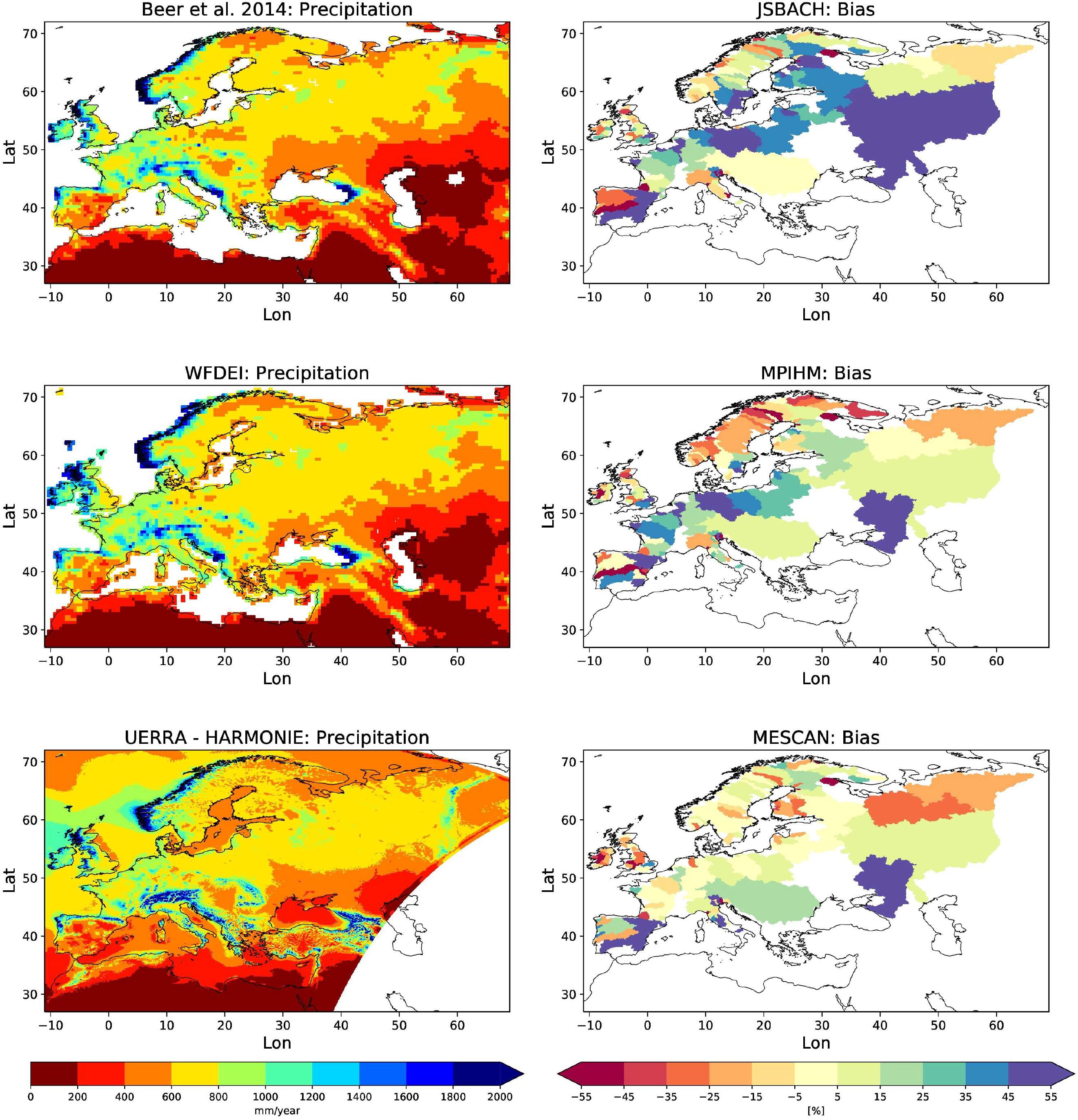
Figure 4. Mean precipitation [mm/a] (left column) and bias in total runoff (right column) of the forcing data for Beer et al. (2014) and JSBACH (1st row), WFDEI and MPI-HM (2nd row), and UERRA-HARMONIE and MESCAN (3rd row), respectively.
The runoff biases shown in Figure 4 impose an upper limit on the accuracy of simulated discharge. Except for rivers with large abstractions of water, biases in total runoff and discharge agree in long-term averages. Therefore, if the KGE of a specific river with a runoff bias c3 is considered, the maximum KGE that can be yielded after simulating the discharge is 1-c3.
Impact of Resolution
First, we consider whether it is beneficial to simulate the discharge at 5 Min. resolution compared to the HD standard resolution of 0.5°. While the answer is trivial for smaller catchments where using the coarse resolution model is not appropriate, this is not obvious for larger rivers.
In Figure 5, monthly discharges of HD5-JSBACH are compared to the 0.5° discharges of HD 1.10 for a few selected rivers. Note that for HD 1.10, we consider not only the grid boxes close to the location of the discharge observations, but also the simulated discharge at the river mouth. The reason is that flow directions at 0.5° were only adjusted for main river paths and at the catchment boundaries, but not for every grid box (Hagemann and Dümenil, 1998). Hence, in some cases, the 0.5° model catchment at a station location may deviate from the actual catchment. Figure 5 shows that it is difficult to judge whether the 5 Min. resolution leads to better discharges or the 0.5° resolution. Despite of some biases, the HD model is able to capture the monthly discharge reasonably well with both resolutions. Only for the Weser, the standard HD model is clearly worse if the grid box near the river gauge is considered. However, this clear discrepancy vanishes if the 0.5° discharge simulated at the river mouth is considered for the reasons mentioned above. Here, the 0.5° model catchment at the station location deviates from the actual catchment within the Weser basin.
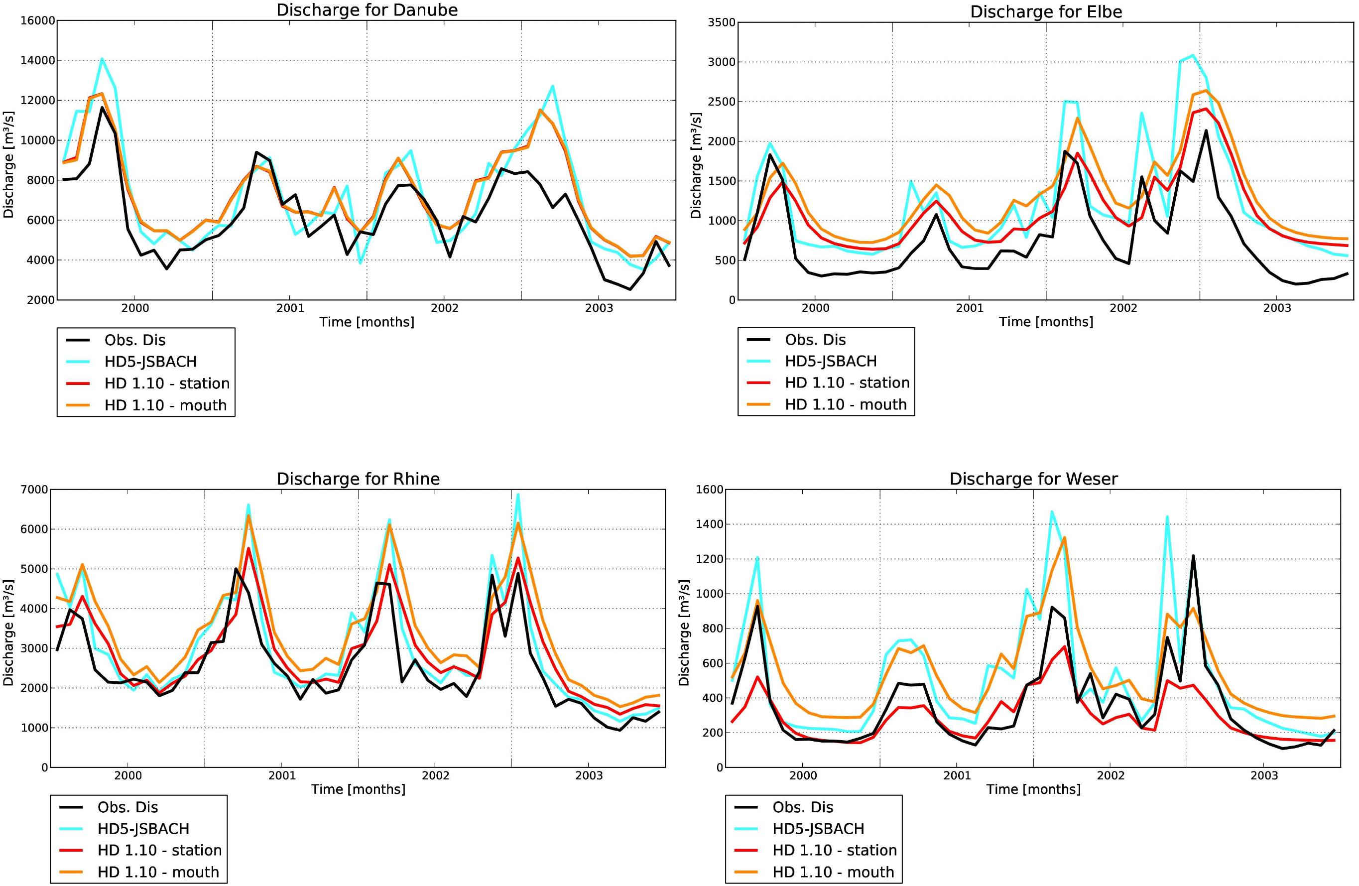
Figure 5. Simulated and observed monthly discharges for selected rivers from 2000–2003. Simulated discharges comprise HD5-JSBACH and HD 1.10 simulations at 0.5° whereat for the latter, discharges close to the discharge gauge and the river mouth are provided. Note that for the Danube, the station is close to the river mouth so that the related discharges are almost identical.
The situation is different when daily discharges are considered as clear improvements are caused by using the higher resolution (Figure 6). With the higher resolution, the variations of many discharge peaks are much better captured than by using the 0.5° resolution. This is also reflected by the increase in the variability ratio that is much closer to the observations with HD5-JSBACH than for HD 1.10 (Table 2). The improved simulation of daily discharges is especially obvious for the Elbe and Weser rivers, but also applies to the Rhine and the Danube. Note that positive runoff biases (see Figure 4) in the JSBACH forcing data limit the overall performance of simulated discharge (cf. discharge bias in Table 2) over the Elbe (runoff bias: 46.1%), Rhine (15.7%), and Weser (43.7%).
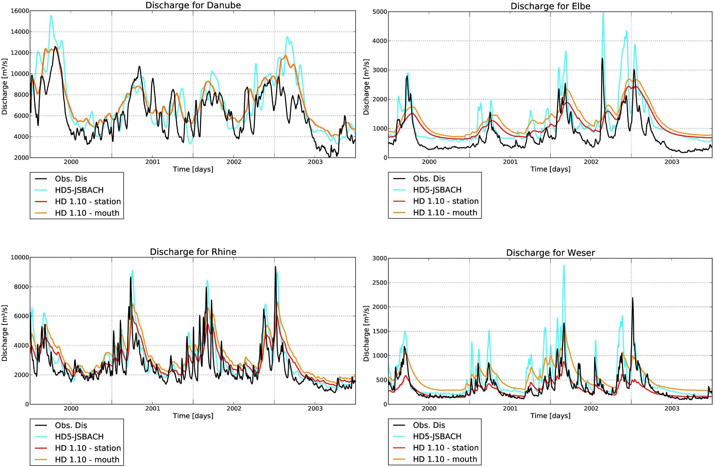
Figure 6. Simulated and observed daily discharges for selected rivers from 2000–2003. Simulated discharges comprise HD5-JSBACH and HD 1.10 simulations at 0.5° whereat for the latter, discharges close to the discharge gauge and the river mouth are provided. Note that for the Danube, the station is close to the river mouth so that the related discharges are almost identical.
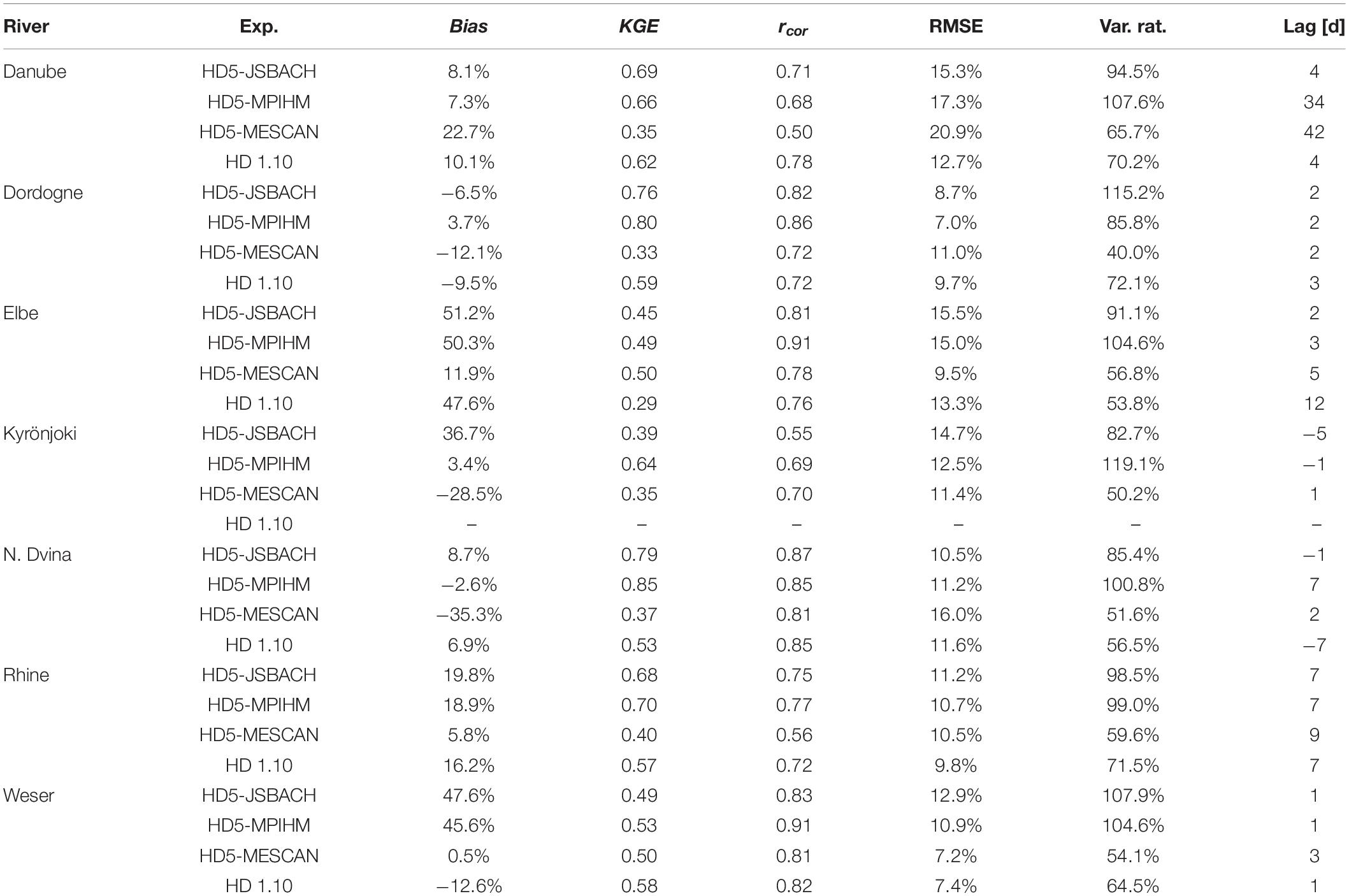
Table 2. Evaluation metrics (2000–2009) for all experiments and those rivers shown in Figures 4–6: Discharge bias, Kling-Gupta Efficiency (KGE), Pearson correlation rcor, normalized RMSE, variability ratio and lag.
Evaluation of 5 Min. Simulations
Figure 7 shows simulated and observed discharges for several rivers across a range of different catchment sizes (shown in brackets with regard to the discharge gauge), ranging from large scale catchments such as the Northern Dvina to small catchments as the Kyrönjoki. The corresponding evaluation metrics are provided in Table 2 for all experiments. As for the rivers shown in Figure 6, the timing of the main peaks is often captured by HD5 for many rivers across Europe, especially by HD5-JSBACH and HD5-MPIHM. In order to evaluate the simulated discharges in a more comprehensive way, various metrics (cf. section “Evaluation Metrics”) were calculated for the different rivers where observed discharge was available within the period of 2000–2009. For the graphical representation, these metrics were allocated to the respective catchment areas.
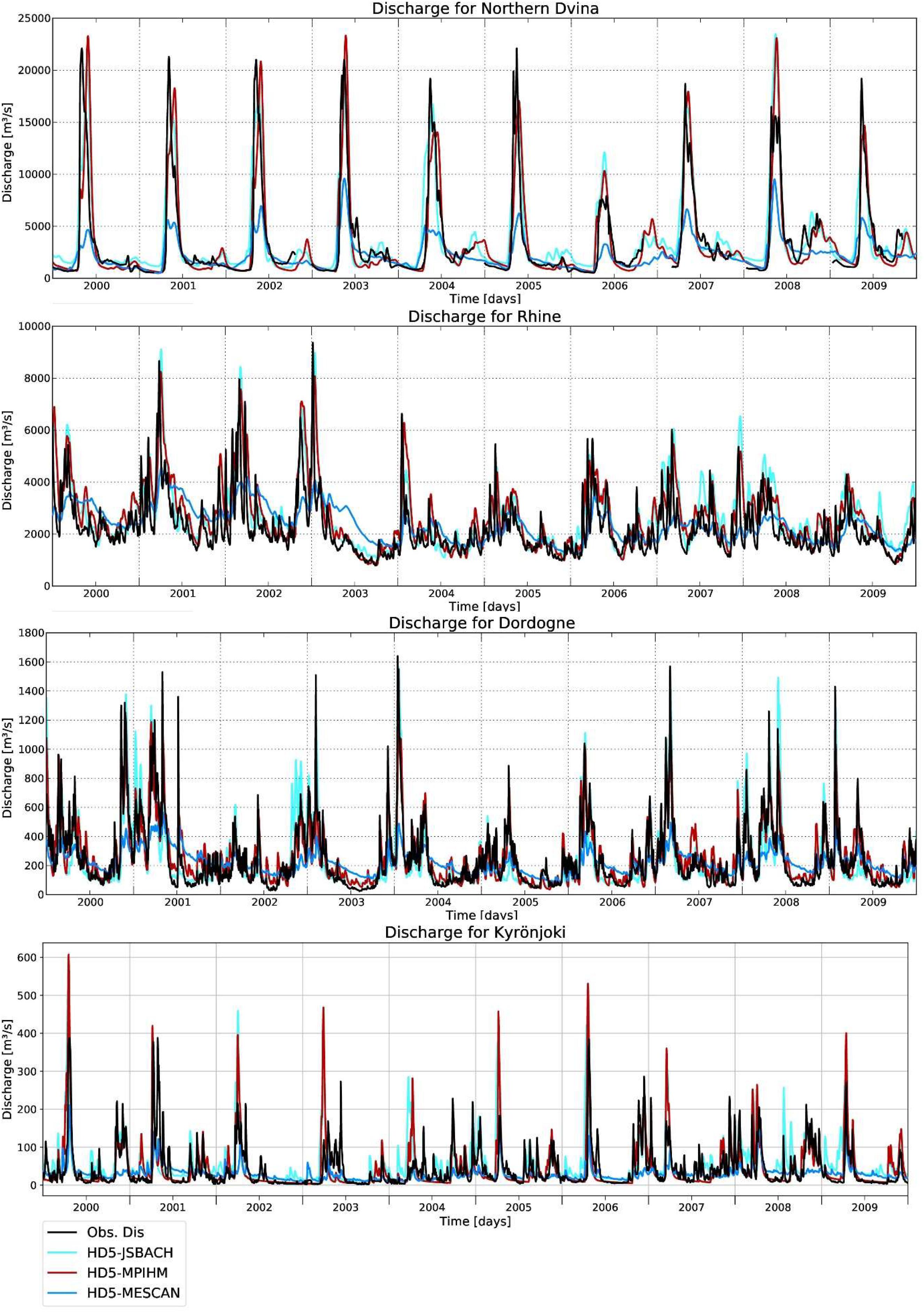
Figure 7. Simulated and observed discharges from 2000–2009 for Northern Dvina (384000 km2), Rhine (160800 km2), Dordogne (14925 km2) and Kyrönjoki (4833 km2). The maximum KGE values are yielded by HD5-MPIHM and are 0.85, 0.70, 0.80, and 0.64, respectively.
Figure 8 (left column) shows the spatial distribution of Kling-Gupta efficiencies (KGEs) across the European catchments for the three experiments. Over northern Russia, Central and Western Europe and Northern Iberia, HD5-JSBACH and HD5-MPIHM yield relatively high KGEs (>0.4, bluish colors). In addition, several rivers flowing into the Baltic Sea show some acceptable performance (>0.3), especially in the southern part. In the contrary, the discharge of many Scandinavian, south Russian and east Spanish rivers is not well represented. HD5-MESCAN shows less good, but still acceptable performance (>0.3) over northern Russia, Central and Western Europe, but an improved simulation of discharge over Scandinavia.
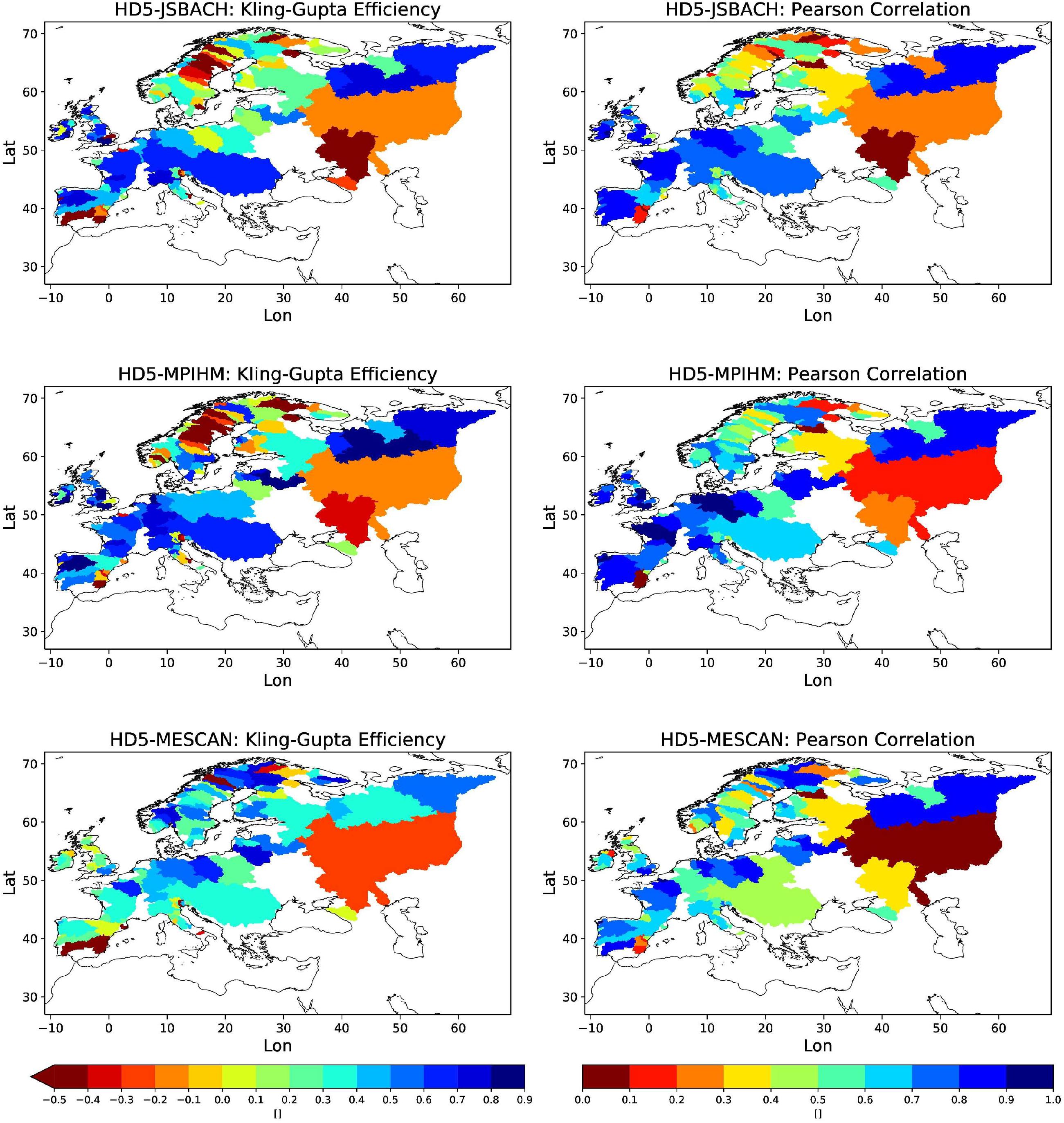
Figure 8. Kling Gupta efficiencies (left column) and Pearson correlations (right column) with the observed daily discharges for HD5-JSBACH (1st row), HD5-MPIHM (2nd row), and HD5-MESCAN (3rd row).
As KGE comprises contributions from correlation, bias and variability terms, correlation rcor, RMSE and the variability ratio of the coefficients of variation are considered in Figure 8 (right column) and Figure 9, left and right column, respectively. Over western Iberia, Central and Western Europe, correlation pattern are similar to the KGE distributions, with HD5-JSBACH and HD5-MPIHM having higher correlations (>0.6) than HD5-MESCAN (>0.4), while all experiments show high correlations (>0.7) over northern Russia. Acceptable correlations (>0.4) are also yielded for many Baltic rivers except for the Newa and some Scandinavian rivers, with HD5-MPIHM being somewhat better than the other two experiments. For the normalized RMSE, HD5-MESCAN tends to have lower values than the other two experiments and has values below 25% for most of the rivers. The other two experiments yield rather high values over some Baltic rivers, but also stay below 25% for many rivers. Again, all experiments have lowest RSME values over northern Russia, western Iberia, Central and Western Europe. A somewhat different picture is obtained for the variability ratios. Here, JSBACH and HD5-MPIHM yield rather good ratios close to one (deviations smaller than 15%) for most rivers in northern Russia, eastern Baltic, western Iberia, Central and Western Europe, but largely overestimate the variability for most Scandinavian rivers and the Don. HD5-MESCAN generally underestimates the variability across all European rivers, except for some Baltic rivers and the Don. Hence, this lower variability induces the main KGE differences to the other two experiments.
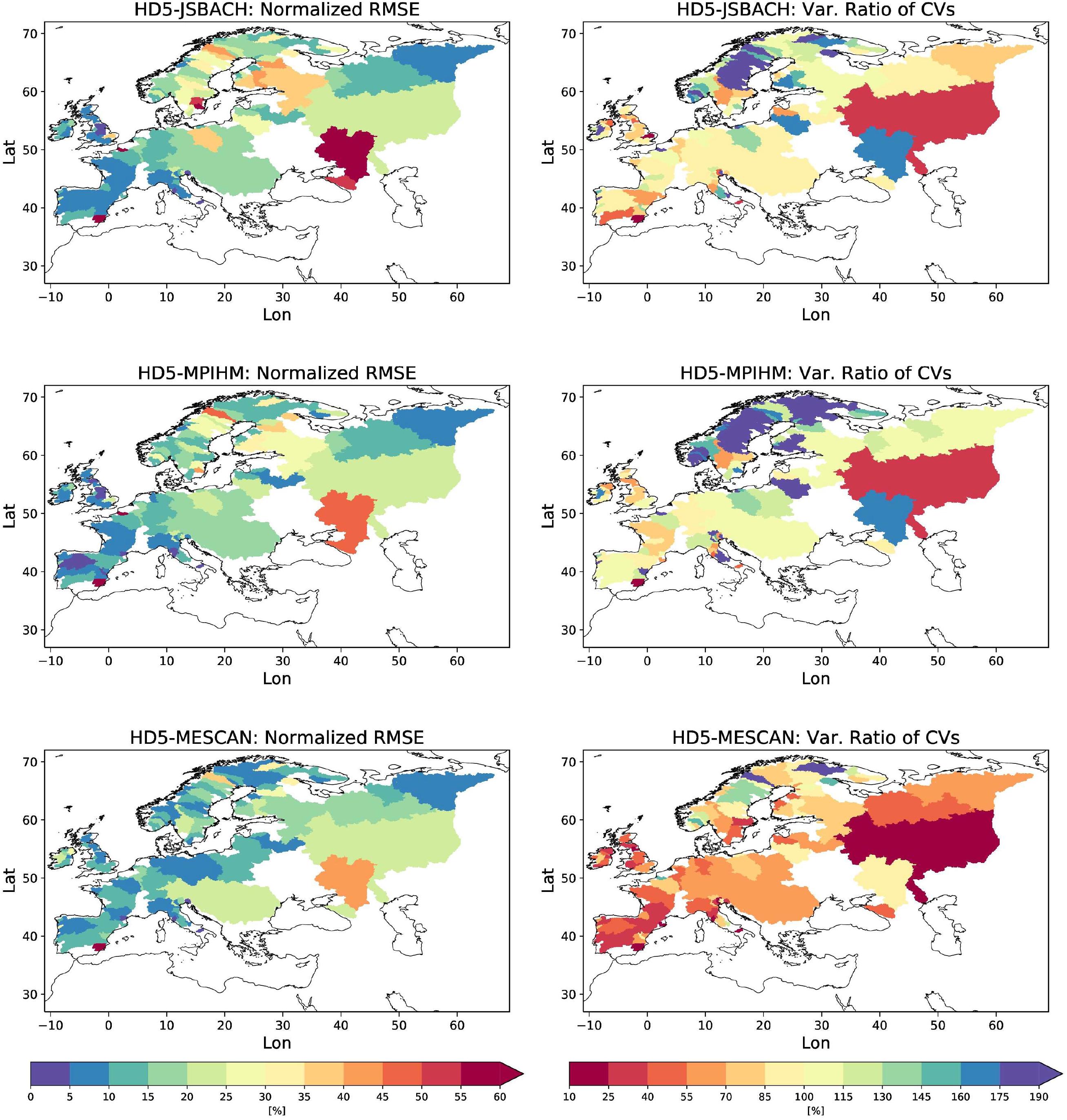
Figure 9. Normalized RSME (left column) and variability ratio of the coefficients of variation (right column) for HD5-JSBACH (1st row), HD5-MPIHM (2nd row), and HD5-MESCAN (3rd row).
To consider the temporal behavior of simulated discharge, the lags compared to the observations are considered in Figure 10. All experiments have low lags (<3 days) for Western Europe and tend to simulate late discharges over Central and especially over Eastern Europe. The HD5-JSBACH discharge generally arrives too early over Northern Europe, while HD5-MESCAN tends to be late across all considered rivers, with some exceptions over Northern Europe. HD5-MPIHM shows much lower lags over Northern Europe, even though it also tends to be too early in this region.
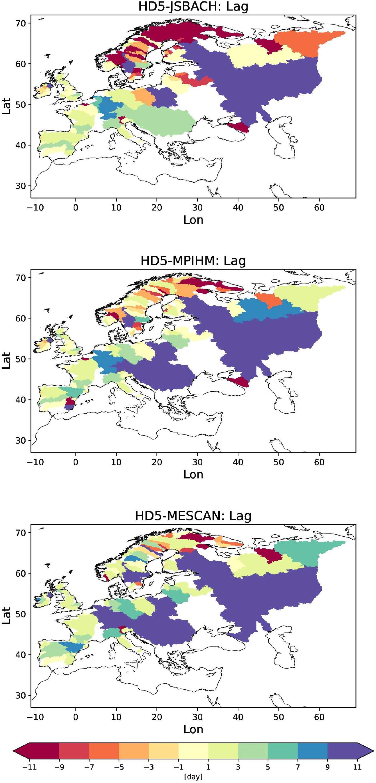
Figure 10. Lags to the observed daily discharges for HD5-JSBACH (upper panel), HD5-MPIHM (middle panel), and HD5-MESCAN (lower panel). A positive lag indicates that the simulated discharge is delayed compared to the observed one.
Discussion of Results
In Scandinavia, especially in Sweden, many rivers are regulated. As this regulation is not regarded in the HD model, its effects can generally not be simulated. A typical example is given for the Indalsaelven (Figure 11). On the one hand, apparent snowmelt induced discharge peaks in spring are simulated, but only weak indications of such peaks occur in the observed time series. On the other hand, there is only little variation in the observed low flow periods, while there is more variability and generally lower discharge in the simulations. This can be interpreted as extractions of water during the snowmelt season and supply of the stored water during low flow periods. It can be noted that rainfall induced discharge peaks outside the snowmelt season are rather well captured by the HD model, e.g., in the second halves of the years 2001, 2004, and 2005 for HD5-JSBACH and HD5-MPIHM.
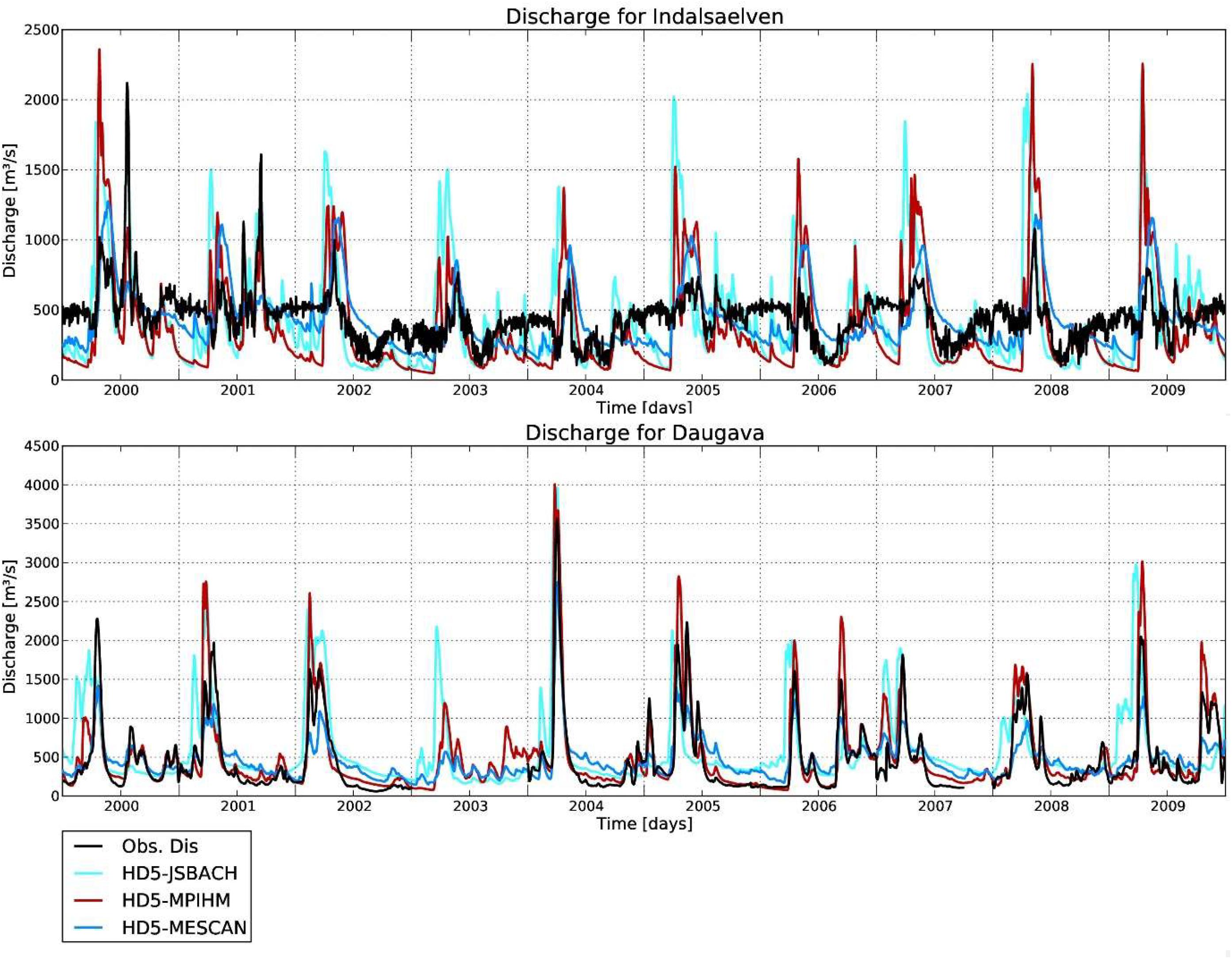
Figure 11. Simulated and observed discharges from 2000–2009 for Indalsälven (25761 km2), and Daugava (64500 km2).
In general, HD5-MESCAN simulates much lower discharge peaks and higher amounts of low flows than the other two experiments. This leads to a worse simulation of daily discharge for many rivers. This is demonstrated for the rivers Rhine and Dordogne (Figure 7) where the discharge peak values are poorly represented by HD5-MESCAN, while the low flows and especially the receding discharge curves after many peaks are strongly overestimated. This erroneous behavior is induced by a different separation of the lateral flow into surface and subsurface runoff in the MESCAN-SURFEX model (Figure 12). This behavior points to deficiencies in its land surface scheme that tends to produce largely under- and overestimated amounts of surface and subsurface runoff, respectively. The biased separation of the lateral flow toward subsurface runoff leads to a general smoothing of the simulated discharge curves. On the one hand, this smoothing leads to a lower variability (Figure 9) than in the observations and the two other experiments. On the other hand, the too strong contribution of slow flow components (subsurface runoff) compared to the fast flow component (surface runoff) leads to a delayed total flow as indicated by the generally larger lags in Figure 10. In a way, the general smoothing is a similar effect as caused by human river regulation. As the erroneous smoothing partially compensates for the missing river regulation process (see above), the simulated discharges are improved for many anthropogenically influenced rivers compared to the other two experiments, especially over Scandinavia. This is also indicated by larger KGE (Figure 8) and lower RSME (Figure 9) than in the other two experiments.
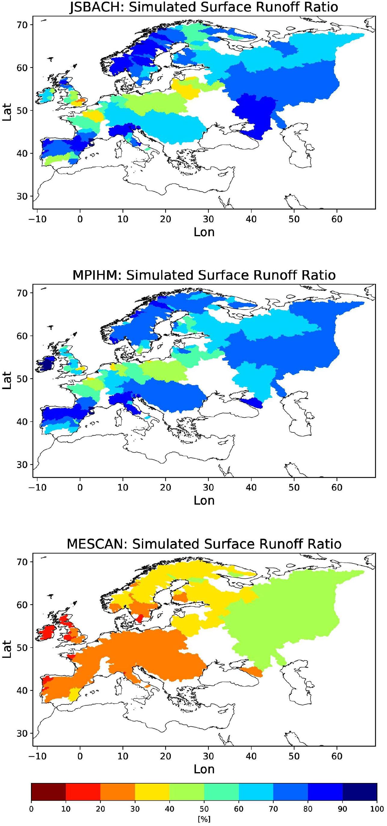
Figure 12. Simulated surface runoff ratio (catchment averaged surface runoff divided by total runoff) for JSBACH (upper panel), MPIHM (middle panel) and MESCAN (lower panel).
For many rivers where the discharge curve is characterized by a snowmelt induced discharge peak in spring, HD5-JSBACH tends to simulate earlier peaks than the other two experiments. This simulated peak often occurs also earlier than in the observations, such as can be seen for the Daugava (Figure 11). As this is not the case for the other two experiments, this points to a deficiency in the JSBACH land surface scheme in simulating a too early snowmelt. As the snowmelt peak in the spring is the dominant characteristic of the discharge curve for these rivers, this deficiency becomes also visible in the lag of the whole discharge time series considered in Figure 10 before.
Since the MESCAN data have a higher spatial resolution compared to other two experiments, it was originally expected that this would yield better-simulated discharge than for the two experiments using 0.5° forcing, particularly over smaller-scale basins with relatively complex terrain like in Scandinavia. With regard to the total bias (Figure 4) and RMSE (Figure 9), this expectation partially holds as HD5-MESCAN shows the lowest error for many rivers. But due to the too low surface runoff ratio, the high resolution advantage is often more than compensated if other metrics are considered (KGE and Pearson correlation in Figure 8, variability ratio of the coefficients of variation in Figure 9), where HD5-MESCAN performs less well than the other two experiments for many rivers, except for Scandinavia (see above).
Summary and Conclusion
In the present study, a well-established discharge model, the HD model, was further developed to be globally applicable at 5 Min. resolution. The improved HD5 model is one of the very first gridded discharge models that is (a) developed for applications in RCSMs, and (b) features a noticeably higher resolution than utilized in previous RCSMs. As the HD5 model shall be applied in climate change studies and over ungauged catchments, no river specific parameter adjustments, e.g., by calibration, were conducted. In order to prepare high-resolution discharge simulations over Europe and the Baltic Sea catchment within a RCSM setup, its initialdevelopment and evaluation wereconducted for a European domain. Note that the HD5 model has already been successfully coupled within the GCOAST-AHOI setup over this domain (Ho-Hagemann et al., submitted). For the validation of the HD5 model, three different methods and datasets were used to derive the required fields of surface and subsurface runoff for the forcing of the HD5 model. Biases in these fields impose an upper limit on the accuracy of simulated discharge that has to be regarded in the evaluation of the HD5 performance. Results from the three respective simulations show that the HD5 model is able to capture the general behavior of discharge for many European rivers, especially in northern Russia, northern Iberia, Western and Central Europe. Several biases could be traced back to deficits in the forcing data, especially with regard to the total amount of runoff, the early snowmelt in JSBACH and the too low surface runoff ratio in MESCAN. For many catchments affected by the deficits of a specific forcing, the corresponding biases are low in those simulations where the respective deficits are not present in the forcing. This indicates that the HD5 model is representing the discharge behavior well for these rivers. Larger deviations of the simulated from the observed discharges occur for rivers that are strongly affected by human impacts such as water abstractions, e.g., for irrigation, and regulation, e.g., by dams. Consequently, for the hydrological modeling of rivers and watersheds that are highly influenced by human activities, related processes need to be implemented into the HD5 model. This includes the implementation of dams and reservoirs (based on available global databases), their management of river flow regulations as well as modules to simulate water withdrawals, e.g., for irrigation.
Apart from lags induced by deficits in the forcing data and the missing representation of human river regulations and water abstractions, some lags may also be introduced if HD5 does not adequately capture the flow regime of a river. This can be caused by the impacts of lakes and wetlands on the river flow, which is currently only simply parameterized (Hagemann and Dümenil, 1998). Here, the Newa is an example whose discharge curve is largely determined by the outflow from the Lake Ladoga. Also a strong meandering, which slows down the flow, or human stream straightening, which accelerates the flow, are not specifically regarded by the model. To overcome such lags, Alwardt (2015) suggested adjusting the flow velocities of the main river flow path of the respective rivers. However, such a correction is not straight forward as it has to be ensured that the lag is caused neither by deficits in the forcing nor by the missing human impact. If a lag were caused by the latter, an adjustment of the flow velocity in the main river flow path would improve the current discharge simulation but may spoil later attempts to include human impacts into the HD model. Potentially, this may be done for rivers where the lag more or less agrees in discharge simulations with different forcings. Using the three forcings of the present study, such a correction may be feasible for the Rhine (lags of 7–9 days) and the Vistula (lags of 15–19 days), but not for the heavy regulated Volga and Don and the lake outflow dominated Newa.
The insufficient availability of daily discharge observations prevents an evaluation of HD5 over all larger European catchments. Figure 13 shows catchments where daily discharge observations were available to us at a downstream station for selected years across the recent decades. Note that we only considered rivers with catchment areas around 3000 km2 or larger. While the situation is rather good in Northern, Western and central Europe, almost no daily data are available for Southern Europe (except for Iberia and northern Italy) and some Eastern European rivers. The spatial coverage of daily data is largest in 1980 and decreases in later decades. Reasons for the data gaps are manifold. Either there are no available downstream stations, the data are not accessible or the available time series are rather short. Often data exists at National authorities, but they were neither making the data freely available nor via GRDC.
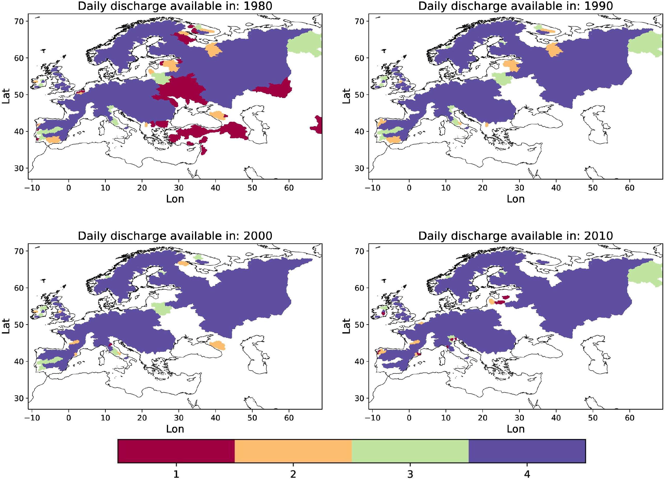
Figure 13. Catchments with daily discharge observations available at a downstream station for more than 90% of days in the years 1980, 1990, 2000, and 2010. Colors indicate the number of years within these 4 years, when discharge data are available.
Such lack of data is not only a south European problem as large-scale international archives of water data are insufficiently equipped in several areas of the world (Hannah et al., 2011). Dixon et al. (2013) pointed out that “globally, funding constraints and changing governmental priorities have resulted in a decline in some river gauging station networks, while concerns about misuse of data, commercial drivers, political sensitivities about transboundary resources and an overarching lack of understanding about the value of river flow information limit the exchange of the hydrological data that is collected.” They further noted that “freshwater environments, their drivers, controls and impacts are not constrained by national boundaries and, hence, international cooperation is vital to provide the information needed to further our understanding of hydrological systems.” Thus, future data policies in Europe should support the open access of discharge data, e.g., via public national data portals or via GRDC.
Despite some recommended developments with regard to human impacts on rivers, our results show that the HD5 model is already well suited for the application within a RCSM. In this respect, an interface to the OASIS coupler (Valcke, 2013) has already been developed which makes the HD model more flexible for coupling purposes. Hence, it may not only be coupled within the GCOAST system (see section “The HD Model”), but also to any other RCM and ocean model via the OASIS coupler. In addition, the comparison of the simulated discharges from the three experiments indicates that the HD5 model is also suitable to evaluate the terrestrial hydrological cycle of climate models or land surface models, especially with regard to the separation of throughfall (rain or snow melt) into surface and subsurface runoff. Currently, such evaluation attempts must be limited to rivers that are not highly influenced by human activities.
Author Contributions
SH carried out the HD model improvements, discharge simulations, analysis of results, and wrote the manuscript. HH-H initiated the study and helped with model adaptations suitable for the coupling within a RCSM. TS generated the MPIHM forcing data. TS and HH-H helped with the analysis and revised the manuscript.
Conflict of Interest
The authors declare that the research was conducted in the absence of any commercial or financial relationships that could be construed as a potential conflict of interest.
Acknowledgments
We are very grateful to Bernhard Lehner (World Wide Fund For Nature) who prepared the used river directions and digital elevation data at 5 Min. for us. We thank the Global Runoff Data Centre for providing most of the discharge observations used in this study. We also thank Sonja van Leuwen (Royal Netherlands Institute for Sea Research) for providing us with some further discharge data from various sources.
Footnotes
- ^ www.gewex.org
- ^ www.eu-watch.org
- ^ https://www.usgs.gov/centers/eros/science/usgs-eros-archive-digital-elevation-hydro1k
- ^ http://maps.elie.ucl.ac.be/CCI/viewer/
- ^ www.uerra.eu
References
Alwardt, C. (2015). Entwicklung eines Aggregierten Modellsystems zur Szenariobasierten Simulation der Wasserhaushalte von Flusseinzugsgebieten, unter Berücksichtigung klimatischer und sozioökonomischer Einflüsse. Ph.D. Thesis, Universität Hamburg, Hamburg.
Anyamba, A., and Tucker, C. J. (2005). Analysis of Sahelian vegetation dynamics using NOAA-AVHRRNDVI data from 19812003. J. Arid. Environ. 63, 596–614. doi: 10.1016/j.jaridenv.2005.03.007
Bazile, E., Abida, R., Szczypta, C., Verelle, A., Soci, C., and Moigne, P. L. (2017). Deliverable D2.9: Ensemble Surface Reanalysis Report. Technical Report No. 607193. Golden, CO: UERRA.
Beer, C., Weber, U., Tomelleri, E., Carvalhais, N., Mahecha, M., and Reichstein, M. (2014). Harmonized European long-term climate data for assessing the effect of changing temporal variability on land-atmosphere CO2 fluxes∗. J. Climate 27, 4815–4834. doi: 10.1175/jcli-d-13-00543.1
Best, M. J., Pryor, M., Clark, D. B., Rooney, G. G., Essery, R. L. H., Ménard, C. B., et al. (2011). The Joint UK Land Environment Simulator (JULES), model description - Part 1: energy and water fluxes. Geosci. Model Dev. 4, 677–699. doi: 10.5194/gmd-4-677-2011
Bierkens, M. F. P., Bell, V. A., Burek, P., Chaney, N., Condon, L. E., David, C. H., et al. (2015). Hyper-resolution global hydrological modelling: what is next? Hydrol. Process. 29, 310–320. doi: 10.1002/hyp.10391
Bouwman, A. F., Bierkens, M. F. P., Griffioen, J., Hefting, M. M., Middelburg, J. J., Middelkoop, H., et al. (2013). Nutrient dynamics, transfer and retention along the aquatic continuum from land to ocean: towards integration of ecological and biogeochemical models. Biogeosciences 10, 1–22. doi: 10.5194/bg-10-1-2013
Breckle, S.-W., and Geldyeva, G. V. (2012). “Dynamics of the Aral Sea in geological and historical times,” in Ecological Studies 218, Aralkum - a Man-Made Desert: The Desiccated Floor of the Aral Sea (Central Asia), eds S.-W. Breckle et al. (Berlin: Springer-Verlag), 13–35. doi: 10.1007/978-3-642-21117-1_2
Bremicker, M. (2000). Das Wasserhaushaltsmodell LARSIM - Modellgrundlagen und Anwendungsbeispiele. Freiburger Schriften zur Hydrologie 11. Freiburg im Breisgau: University of Freiburg im Breisgau.
Daewel, U., and Schrum, C. (2017). Low-frequency variability in North Sea and Baltic Sea identified through simulations with the 3-D coupled physical–biogeochemical model ECOSMO. Earth Syst. Dyn. 8:801. doi: 10.5194/esd-8-801-2017
Decharme, B., Martin, E., and Faroux, S. (2013). Reconciling soil thermal and hydrological lower boundary conditions in land surface models. J. Geophys. Res. Atmos. 118, 7819–7834. doi: 10.1002/jgrd.50631
Dee, D. P., Uppala, S. M., Simmons, A. J., Berrisford, P., Poli, P., Kobayashi, S., et al. (2011). The ERA-interim reanalysis: configuration and performance of the data assimilation system. Quart. J. Roy. Meteor. Soc. 137, 553–597. doi: 10.1002/qj.828
Dell’Aquila, A., Calmanti, S., Ruti, P., Struglia, M., Pisacane, G., Carillo, A., et al. (2012). Effects of seasonal cycle fluctuations in an a1b scenario over the euro-mediterranean region. Clim. Res. 52, 135–157. doi: 10.3354/cr01037
Dixon, H., Rodda, J., Jenkins, A., Demuth, S., and Looser, U. (2013). “Sharing water observations: turning local data into global information,” in Free Flow - Reaching Water Security Through Cooperation, eds J. Griffiths and R. Lambert (France: UNESCO).
Donnelly, C., Andersson, J. C. M., and Arheimer, B. (2016). Using flow signatures and catchment similarities to evaluate the e-hype multi-basin model across europe. Hydrol. Sci. J. 61, 255–273. doi: 10.1080/02626667.2015.1027710
Ekici, A., Beer, C., Hagemann, S., Boike, J., Langer, M., and Hauck, C. (2014). Simulating high-latitude permafrost regions by the JSBACH terrestrial ecosystem model. Geosci. Model Dev. 7, 631–647. doi: 10.5194/gmd-7-631-2014
Elizalde, A. (2011). The Water Cycle in the Mediterranean Region and the Impacts of Climate Change. Ph.D. Thesis. MPI for Meteorology, Hamburg, doi: 10.17617/2.1216556
Epule, E. T., Peng, C., Lepage, L., and Chen, Z. (2014). The causes, effects and challenges of Sahelian droughts: a critical review. Reg. Environ. Change 14, 145–156. doi: 10.1007/s10113-013-0473-z
Expósito, A. (2018). Irrigated agriculture and the cost recovery principle of water services: assessment and discussion of the case of the Guadalquivir river basin (Spain). Water 10:1338. doi: 10.3390/w10101338
Flato, G., Marotzke, J., Abiodun, B., Braconnot, P., Chou, S., Collins, W., et al. (2013). “Evaluation of climate models,” in Climate Change 2013: The Physical Science Basis. Contribution of Working Group I to the Fifth Assessment Report of the Intergovernmental Panel on Climate Change, eds T. Stocker, D. Qin, G.-K. Plattner, M. Tignor, S. Allen, J. Boschung, et al. (Cambridge: Cambridge University Press), 741–866.
Flörke, M., Kynast, E., Barlund, I., Eisner, S., Wimmer, F., and Alcamo, J. (2013). Domestic and industrial water uses of the past 60 years as a mirror of socio-economic development: a global simulation study. Glob. Environ. Change 23, 144–156. doi: 10.1016/j.gloenvcha.2012.10.018
Giorgetta, M. A., Jungclaus, J., Reick, C. H., Legutke, S., Bader, J., Böttinger, M., et al. (2013). Climate and carbon cycle changes from 1850 to 2100 in MPI-ESM simulations for the Coupled Model Intercomparison Project phase 5. J. Adv. Model. Earth Syst. 5, 572–597. doi: 10.1002/jame.20038
Guimberteau, M., Drapeau, G., Ronchail, J., Sultan, B., Polcher, J., Martinez, J.-M., et al. (2012). Discharge simulation in the sub-basins of the amazon using ORCHIDEE forced by new datasets. Hydrol. Earth Syst. Sci. 16, 911–935. doi: 10.5194/hess-16-911-2012
Gupta, H. V., Kling, H., Yilmaz, K. K., and Martinez, G. F. (2009). Decomposition of the mean squared error and NSE performance criteria: implications for improving hydrological modelling. J. Hydrol. 377, 80–91. doi: 10.1016/j.jhydrol.2009.08.003
Haddeland, I., Clark, D. B., Franssen, W., Ludwig, F., Voß, F., Arnell, N. W., et al. (2011). Multimodel estimate of the global terrestrial water balance: setup and first results. J. Hydrometeorol. 12, 869–884. doi: 10.1175/2011jhm1324.1
Hagemann, S. (2002). An Improved Land Surface Parameter Dataset for Global and Regional Climate Models. Max Planck Institute for Meteorology Report No. 336. Hamburg: MPI for Meteorology.
Hagemann, S., Chen, C., Clark, D. B., Folwell, S., Gosling, S. N., Haddeland, I., et al. (2013). Climate change impact on available water resources obtained using multiple global climate and hydrology models. Earth Syst. Dyn. 4, 129–144. doi: 10.5194/esd-4-129-2013
Hagemann, S., and Dümenil, L. (1998). A parametrization of the lateral waterflow for the global scale. Climate Dyn. 14, 17–31. doi: 10.1007/s003820050205
Hagemann, S., and Dümenil Gates, L. (2001). Validation of the hydrological cycle of ECMWF and NCEP reanalyses using the MPI hydrological discharge model. J. Geophys. Res. D 106, 1503–1510. doi: 10.1029/2000JD900568
Hannah, D. M., Demuth, S., van Lanen, H. A. J., Looser, U., Prudhomme, C., Rees, G., et al. (2011). Large-scale river flow archives: importance, current status and future needs. Hydrol. Process. 25, 1191–1200. doi: 10.1002/hyp.7794
Harding, R., Best, M., Blyth, E., Hagemann, S., Kabat, P., Tallaksen, L. M., et al. (2011). WATCH: current knowledge of the terrestrial global water cycle. J. Hydrometeorol. 12, 1149–1156. doi: 10.1175/jhm-d-11-024.1
Hordoir, R., and Meier, H. E. M. (2010). Freshwater fluxes in the Baltic Sea: a model study. J. Geophys. Res. 115:C08028. doi: 10.1029/2009jc005604
Hordoir, R., Polcher, J., Brun-Cottan, J.-C., and Madec, G. (2008). Towards a parametrization of river discharges into ocean general circulation models: a closure through energy conservation. Climate Dyn. 31, 891–908. doi: 10.1007/s00382-008-0416-4
Jungclaus, J. H., Keenlyside, N., Botzet, M., Haak, H., Luo, J.-J., Latif, M., et al. (2006). Ocean circulation and tropical variability in the coupled model ECHAM5/MPI-OM. J. Climate 19:3952. doi: 10.1175/jcli3827.1
Khublaryan, M. G. (2009). “Water resources for sustainable development, with particular reference to Russia,” in Area Studies (Regional Sustainable Development Review): Russia, Vol.I, ed. N. P. Laverov (Oxford: Eolss Publishers Co. Ltd), 81–94.
Kling, H., Fuchs, M., and Paulin, M. (2012). Runoff conditions in the upper Danube basin under an ensemble of climate change scenarios. J. Hydrol. 42, 264–277. doi: 10.1016/j.jhydrol.2012.01.011
Kotlarski, S., Keuler, K., Christensen, O. B., Colette, A., Déqué, M., Gobiet, A., et al. (2014). Regional climate modeling on European scales: a joint standard evaluation of the EURO-CORDEX RCM ensemble. Geosci. Model Dev. 7, 1297–1333. doi: 10.5194/gmd-7-1297-2014
Larsen, M. A. D., Refsgaard, J. C., Drews, M., Butts, M. B., Jensen, K. H., Christensen, J. H., et al. (2014). Results from a full coupling of the HIRHAM regional climate model and the MIKE SHE hydrological model for a danish catchment. Hydrol. Earth Syst. Sci. 18, 4733–4749. doi: 10.5194/hess-18-4733-2014
Lawrence, D. M., Oleson, K. W., Flanner, M. G., Thornton, P. E., Swenson, S. C., Lawrence, P. J., et al. (2011). Parameterization improvements and functional and structural advances in version 4 of the community land model. J. Adv. Model. Earth Syst. 3:M03001. doi: 10.1029/2011MS00045
Lee, J.-W., Hong, S.-Y., Kim, J.-E. E., Yoshimura, K., Ham, S., and Joh, M. (2015). Development and implementation of river-routing process module in a regional climate model and its evaluation in korean river basins. J. Geophys. Res. Atmos. 120, 4613–4629. doi: 10.1002/2014JD022698
Lehmann, A., and Hinrichsen, H.-H. (2000). On the thermohaline variability of the baltic sea. J. Mar. Syst. 25, 333–357. doi: 10.1016/s0924-7963(00)00026-9
Lehner, B., Verdin, K., and Jarvis, A. (2006). HydroSHEDS Technical Documentation. Washington, DC: World Wildlife Fund US.
Lindström, G., Pers, C., Rosberg, J., Strömqvist, J., and Arheimer, B. (2010). Development and testing of the HYPE (Hydrological Predictions for the Environment) water quality model for different spatial scales. Hydrol. Res. 41, 295–319. doi: 10.2166/nh.2010.007
López López, P., Wanders, N., Schellekens, J., Renzullo, L. J., Sutanudjaja, E. H., and Bierkens, M. F. P. (2016). Improved large-scale hydrological modelling through the assimilation of streamflow and downscaled satellite soil moisture observations. Hydrol. Earth Syst. Sci. 20, 3059–3076. doi: 10.5194/hess-20-3059-2016
Lorenz, P., and Jacob, D. (2014). BALTIMOS — a coupled modelling system for the Baltic Sea and its drainage basin. Theor. Appl. Climatol. 118:715. doi: 10.1007/s00704-014-1276-y
Marzeion, B., Levermann, A., and Mignot, J. (2007). The role of stratification-dependent mixing for the stability of the Atlantic overturning in a global climate model. J. Phys. Oceanogr. 37, 2672–2681. doi: 10.1175/2007jpo3641.1
Masson, V., Moigne, P. L., Martin, E., Faroux, S., Alias, A., Alkama, R., et al. (2013). The SURFEXv7.2 land and ocean surface platform for coupled or offline simulation of earth surface variables and fluxes. Geosci. Model Dev. 6, 929–960. doi: 10.5194/gmd-6-929-2013
Mauser, W., and Bach, H. (2009). PROMET - Large scale distributed hydrological modelling to study the impact of climate change on the water flows of mountain watersheds. J. Hydrol. 376, 362–377. doi: 10.1016/j.jhydrol.2009.07.046
Merchán, D., Causapé, J., and Abrahao, R. (2013). Impact of irrigation implementation on hydrology and water quality in a small agricultural basin in Spain. Hydrol. Sci. J. 58, 1400–1413. doi: 10.1080/02626667.2013.829576
Milly, P. C. D., Malyshev, S. L., Shevliakova, E., Dunne, K. A., Findell, K. L., Gleeson, T., et al. (2014). An enhanced model of land water and energy for global hydrologic and earth-system studies. J. Hydrometeorol. 15, 1739–1761. doi: 10.1175/jhm-d-13-0162.1
Nash, J., and Sutcliffe, J. (1970). River flow forecasting through conceptual models part I - A discussion of principles. J. Hydrol. 10, 282–290. doi: 10.1016/0022-1694(70)90255-6
Oki, T., and Sud, Y. C. (1998). Earth Interact. 2, 1–37. doi: 10.1175/1087-35621998002<0001:dotrip<2.3.co;2
Österblom, H., Hansson, S., Larsson, U., Hjerne, O., Wulff, F., Elmgren, R., et al. (2007). Human-induced trophic cascades and ecological regime shifts in the Baltic Sea. Ecosystems 10, 877–889. doi: 10.1007/s10021-007-9069-0
Ridal, M., Olsson, E., Unden, P., Zimmermann, K., and Ohlsson, A. (2017). Deliverable D2.7: HARMONIE Reanalysis Report of Results and Dataset. Resarch Report No. 607193 Golden, CO: UERRA.
Roeckner, E., Bäuml, G., Bonaventura, L., Brokopf, R., Esch, M., Giorgetta, M., et al. (2003). The Atmospheric General Circulation Model ECHAM 5. PART I: Model Description. Max Planck Institute for Meteor. Report No. 349, MPI for Meteorology, Hamburg.
Samaniego, L., Kumar, R., and Attinger, S. (2010). Multiscale parameter regionalization of a grid-based hydrologic model at the mesoscale. Water Resour. Res. 46:W05523. doi: 10.1029/2008WR007327
Sein, D. V., Mikolajewicz, U., Gröger, M., Fast, I., Cabos, W., Pinto, J. G., et al. (2015). Regionally coupled atmosphere-ocean-sea ice-marine biogeochemistry model ROM: 1. description and validation. J. Adv. Model. Earth Syst. 7, 268–304. doi: 10.1002/2014ms000357
Senatore, A., Mendicino, G., Gochis, D. J., Yu, W., Yates, D. N., and Kunstmann, H. (2015). Fully coupled atmosphere-hydrology simulations for the central mediterranean: impact of enhanced hydrological parameterization for short and long time scales. J. Adv. Model. Earth Syst. 7, 1693–1715. doi: 10.1002/2015ms000510
Sevault, F., Somot, S., Alias, A., Dubois, C., Lebeaupin-Brossier, C., Nabat, P., et al. (2014). A fully coupled mediterranean regional climate system model: design and evaluation of the ocean component for the 1980-2012 period. Tellus A 66:23967. doi: 10.3402/tellusa.v66.23967
Shrestha, P., Sulis, M., Masbou, M., Kollet, S., and Simmer, C. (2014). A scale-consistent terrestrial systems modeling platform based on COSMO. CLM, and ParFlow. Mon. Weather Rev. 142, 3466–3483. doi: 10.1175/mwr-d-14-00029.1
Sitz, L. E., Sante, F. D., Farneti, R., Fuentes-Franco, R., Coppola, E., Mariotti, L., et al. (2017). Description and evaluation of the earth system regional climate model (Reg CM-ES). J. Adv. Model. Earth Syst. 9, 1863–1886. doi: 10.1002/2017ms000933
Sorooshian, S., Lawford, R., Try, P., Rossow, W., Roads, J., Polcher, J., et al. (2005). Water and energy cycles: investigating the links. WMO Bull. 54, 58–64. doi: 10.3389/fmicb.2016.00214
Stacke, T., and Hagemann, S. (2012). Development and evaluation of a global dynamical wetlands extent scheme. Hydrol. Earth Syst. Sci. 16, 2915–2933. doi: 10.5194/hess-16-2915-2012
Thurow, F. (1997). Estimation of the total fish biomass in the Baltic Sea during the 20th century. ICES J. Mar. Sci. 54, 444–461. doi: 10.1006/jmsc.1996.0195
Valcke, S. (2013). The OASIS3 coupler: a european climate modelling community software. Geosci. Model Dev. 6, 373–388. doi: 10.5194/gmd-6-373-2013
Väli, G., Meier, H. E. M., and Elken, J. (2013). Simulated halocline variability in the Baltic Sea and its impact on hypoxia during 1961-2007. J. Geophys. Res. Oceans 118, 6982–7000. doi: 10.1002/2013jc009192
Van Der Knijff, J. M., Younis, J., and Roo, A. P. J. D. (2010). LISFLOOD: a GIS-based distributed model for river basin scale water balance and flood simulation. Int. J. Geogr. Inf. Sci. 24, 189–212. doi: 10.1080/13658810802549154
Warszawski, L., Frieler, K., Huber, V., Piontek, F., Serdeczny, O., and Schewe, J. (2014). The inter-sectoral impact model intercomparison project (ISIMIP): project framework. Proc. Natl. Acad. Sci. U.S.A. 111, 3228–3232. doi: 10.1073/pnas.1312330110
Weedon, G. P., Balsamo, G., Bellouin, N., Gomes, S., Best, M. J., and Viterbo, P. (2014). The WFDEI meteorological forcing data set: WATCH Forcing Data methodology applied to ERA-Interim reanalysis data. Water Resour. Res. 50, 7505–7514. doi: 10.1002/2014WR015638
Weedon, G. P., Gomes, S., Viterbo, P., Shuttleworth, W. J., Blyth, E., Österle, H., et al. (2011). Creation of the WATCH Forcing Data and its use to assess global and regional reference crop evaporation over land during the twentieth century. J. Hydrometeorol. 12, 823–848. doi: 10.1175/2011JHM1369.1
Keywords: discharge modeling, large-scale river routing, daily runoff, high resolution, Europe
Citation: Hagemann S, Stacke T and Ho-Hagemann HTM (2020) High Resolution Discharge Simulations Over Europe and the Baltic Sea Catchment. Front. Earth Sci. 8:12. doi: 10.3389/feart.2020.00012
Received: 17 October 2018; Accepted: 20 January 2020;
Published: 13 February 2020.
Edited by:
Martin Stendel, Danish Meteorological Institute (DMI), DenmarkReviewed by:
Deniz Bozkurt, University of Chile, ChileXander Wang, University of Prince Edward Island, Canada
Copyright © 2020 Hagemann, Stacke and Ho-Hagemann. This is an open-access article distributed under the terms of the Creative Commons Attribution License (CC BY). The use, distribution or reproduction in other forums is permitted, provided the original author(s) and the copyright owner(s) are credited and that the original publication in this journal is cited, in accordance with accepted academic practice. No use, distribution or reproduction is permitted which does not comply with these terms.
*Correspondence: Stefan Hagemann, stefan.hagemann@hzg.de
 Stefan Hagemann
 Tobias Stacke1,2