 Eleni Stavropoulou1
 Edward Andò1
 Emmanuel Roubin1
 Nicolas Lenoir1,2
 Alessandro Tengattini1,2
 Matthieu Briffaut1
 Pierre Bésuelle1*
- 1Univ. Grenoble Alpes, CNRS, Grenoble INP, 3SR, Grenoble, France
- 2Institute Laue-Langevin, Grenoble, France
The Callovo-Oxfordian claystone is a material with notoriously complex hydro-mechanical behaviour. Combined neutron and x-ray tomography modalities are used for the first time to characterise the dynamics of water absorption in this material by comparing material deformation as well as water arrival. Exploiting recent work on multimodal registration, neutron, and x-ray datasets are registered pairwise into a common coordinate system, meaning that a vector-valued field (i.e., neutron and x-ray reconstructed values) is available for each timestep, essentially making this a 5D dataset. The ability to cross-plot each field into a joint histogram (an inherent input into the registration) allows an improved identification of mineral phases in this complex material. Material deformation obtained from the application of Digital Volume Correlation on the x-ray timeseries data is locally compared to changes in water content available from the neutrons, opening the way toward a quantitative description of the hydro-mechanics of this process.
1. Introduction
The beginning of the study of clay-rich formations as a potential geological barrier for the storage of nuclear waste dates back to a couple of decades (Bonin, 1998; Andra, 2005; Delay et al., 2010). In France, the Callovo Oxfordian claystone (COx) is being studied by Andra (The French radioactive Waste Management Agency) through an impressive volume of in-field and lab-scale work. This claystone's properties (low permeability, self-sealing properties) make it a favourable host rock, however, the complex couplings that govern its hydromechanical behaviour are still under investigation.
The mechanical response of the COx claystone is strongly related to its water content (Armand et al., 2017), the variation of which (drying-wetting process) has been related to the modification of its microstructure (Montes et al., 2004; Robinet et al., 2012). The non-linear response observed at high relative humidity has not only been related to damage (Chiarelli et al., 2000; Escoffier, 2002), but also to the non-linear swelling of the clay mineral (Wang et al., 2014) under these conditions. The swelling properties of the Callovo Oxfordian are linked to the presence of smectite in the clay matrix, which is very sensitive to water content changes and triggers swelling at high degrees of relative humidity (Homand et al., 2006).
A number of authors have studied the kinematics of clay-rich rocks due to wetting using different imaging tools, such as environmental scanning electron microscopy (ESEM) (Montes et al., 2004; Wang et al., 2015), scanning electron microscopy (SEM) (Desbois et al., 2017), optical microscopy (Bornert et al., 2010), or x-ray tomography (Lenoir et al., 2007). All these methods allow structural modification due to water content changes to be captured and consequently the computation of strains, however, they do not provide direct information related to water presence.
Moisture change in geomaterials has been investigated through neutron tomography, since neutrons are sensitive to hydrogen (due to their high attenuation of cold neutrons itself due to elastic scattering of neutrons). DiStefano et al. (2017) measured imbibition into a shale using in-situ neutron imaging. Combined x-ray and neutron tomographies on shales Chiang et al. (2018) indicate that the combination of techniques allows a better identification of the composition of these complex materials. Stavropoulou et al. (2019) combined x-ray tomography and neutron radiography to study wate imbibition in COx (albeit on twin samples) linking the cracking and propagation to the water penetration. Even though interesting trends have been revealed, this study is limited by the use of similar but different samples, meaning that the characterisation of a mechanism linking crack opening and water penetration is difficult to quantify locally.
This paper presents a significant technical evolution of Stavropoulou et al. (2019) with the analysis of a wetting test on Callovo Oxfordian claystone using a simultaneous x-ray and neutron tomography on the same sample.
2. Experimental Setup
2.1. Sample Preparation
For sample preparation, a fresh claystone core was used (EST57917, h = 300 mm, d = 120 mm) extracted from a depth of 490 m. The samples have been cut to a cylindrical shape (h = d = 20 mm) using a wire saw in neighbouring locations within the core. The average water content () has been measured after drying at 105°C for at least 24 h equal to 6.54 %, a value a bit lower than what has been reported by Conil et al. (2018). This paper presents the analysis of the first sample of a series, the vertical axis of which is parallel to the bedding plane of the claystone.
Even though the experimental equipment that was designed and used for this study allows a confining pressure to be applied within a pressure vessel, this particular test is performed without confining pressure (other than that offered by the latex membrane). The experimental setup is shown in Figure 1. The sample is positioned on top of an aluminium base through which the water is supplied to the bottom of the sample. In order to ensure water arrival, a double hole and spiral passage is manufactured and placed on top of the aluminium base (see later Figure 3 bottom), while the uniform distribution of the water supply to the sample is achieved using a filter paper at its bottom.
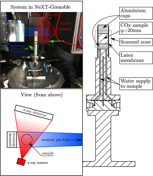
Figure 1. Design of experimental used in this work. Left: photo of setup set up on NeXT-Grenoble scanner, with the sample set up on pedestal. Right: illustrative top view (scales and angles not exact) showing the dual-modality scanning setup on NeXT-Grenoble.
An initial tomography (numbered 001) with both modalities (details in next section) is acquired of the sample before starting water imbibition. Thereafter the air is vacuumed out of the water supply lines, and the imaging systems are readied. Water is supplied to the sample and back-to-back scans are immediately started. Tomographies are recorded back-to-back starting from number 002, which is used as the reference state for the following analysis.
2.2. Neutron and x-Ray Tomography Acquisition
X-ray and neutron tomographies were acquired simultaneously on NeXT-Grenoble (Tengattini et al., 2017, 2019), which is equipped with an almost-parallel cold neutron beam and now a micro-focus x-ray setup with a flat panel detector. The addition of the x-ray setup is a significant improvement from our preliminary study Stavropoulou et al. (2019) where twin samples were required for separate scanning with the two different modalities (neutrons and x-rays).
For the x-ray tomographies, the geometric pixel size is 42.70 μm/px. The Hamamatsu L-12161-07 x-ray source is operated at 140 kV and 130 μA. The source focuses its electron stream into a small point, creating a divergent conical beam. The Varex 2530HE Flat-panel detector records the beam with an exposure time of 1/9 s behind a B4C filter. Each radiograph is the result of averaging 5 exposures.
Regarding neutron tomographies, NeXT-Grenoble is on a cold source, and the beam reaches the sample after going through a 30 mm diameter pinhole (with no filter). A very large collimation distance is used (around 10 m), meaning that at the sample the beam is practically parallel. A camera-mirror-scintillator system is used to detect neutrons, with a 25 x 25 mm field of view. The Hamamastu Orca Flash V2 is equipped with Canon 180 mm F3.5 optics. The camera is used in binning 4 yielding a pixel size of approximately 50 μm/px. The camera is set to 0.6 s exposure. The scintillator used is a 50 μm thick LiF.
The x-ray and neutron acquisitions are controlled together by a proprietary RX-Solutions system. For both modalities 896 radiographs are acquired meaning scans last around 8 min. The two beams are oriented roughly perpendicular to each other (but not exactly at 90° to optimise the use of the x-ray cone beam).
During the test an interruption was necessary, meaning that seven scans are missing around the middle of the test. Due to probable neutron capture effects some greyscale corrections (detailed below) were necessary particularly after this pause.
3. Data Analysis
Both series of simultaneously acquired x-ray and neutron tomographies are reconstructed individually using the usual Filtered Back-Projection technique: the Feldkamp algorithm for the divergent x-rays and a parallel algorithm for the neutrons. The software used is RX-Solutions' UniCT, and a software correction for both beam-hardening and ring correction is applied. The resulting 3D fields of reconstructed values lumped attenuation coefficients for both modalities (henceforth referred to as μx for x-rays and μn for neutrons) are then saved on a 16-bit data range (scaling factors are kept constant for each modality).
In order to be able to simply compare noise levels between the two modalities, both tomographies of state 002 are linearly rescaled such that the mean value of the air (background) is 0.0 and the mean value of the clay matrix (foreground) is 1.0. After rescaling, the standard deviation of the background for μn is 0.069 and 0.011 for μx. The Signal to Noise Ratio can coarsely be taken as the reciprocal of these quantities since the claystone is scaled to 1.0, giving SNRn = 14.5 and SNRx = 90.
In order to denoise the μn field, each field is smoothed using the bilateral filter (Tomasi and Manduchi, 1998) offered in the Insight Toolkit (ITK) (Yoo et al., 2002) with a σdomain = 1 and σrange = 3,000. According to the definition above, the SNRn-bilateral significantly increases to 36, at the cost of a small loss of sharpness. In what follows, these filtered images will be used for μn.
Since this study is mostly concerned with the entry of water into the claystone, the SNR is also computed taking the pure clay matrix as background (see later for the computation of its greylevel) and the water as the phase of interest. For safety the standard deviation of greyvalues is computed on the aluminium top cap (since the claystone has natural variations). This yields an =125 and =37, which confirms the significant interest in the use of neutron tomography for following water.
3.1. Multimodal Registration
With a long time-series of both neutron and x-ray tomography it is very useful to be able to have a common coordinate system. If an exact match between μx and μn measurements can be achieved, the 3D data collected can be thought of as a vector-valued 3D field, where every voxel contains a value of μx and μn. Within the same modality the image registration problem can be written as the minimisation of the difference between the greyvalues, however since different modalities offer different contrast mechanisms, this subtraction no longer makes sense.
To this end a “multimodal registration” tool is used as first presented in Tudisco et al. (2017) and subsequently developed in Roubin et al. (2019). The inherent linearisation of the problem requires a good initial guess of the solution for registration to converge. The μx and μn volumes collected during this campaign are not easy to correlate, and the final result was found to be sensitive to the initial guess. A graphical user interface was implemented to allow an initial alignment by eye to be done, as illustrated in Figure 2.
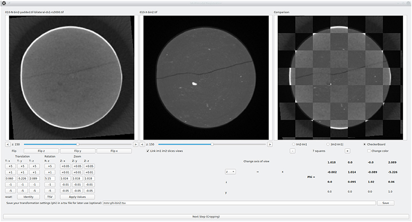
Figure 2. Example of graphical tool (available in spam) developed in Qt allowing an accurate initial Φ to be manually applied to the neutrons to initialise the multimodal registration as close as possible to the correct solution. Top row: Horizontal slices through tomographies: (left) neutron (middle) x-rays (right) “checkerboard” allowing comparison. Bottom row: (left) Buttons to apply displacements, rotations and zooms to left image (middle) slice view settings (right) current Φ matrix. This software is free software and is included in the ‘‘spam” python package.
The transformation to be applied to the neutron image by trilinear interpolation is described as a “linear deformation function” Φ (represented as a 4 × 4 matrix), meaning that rotations, shear and zoom changes of shapes can be described as well as sub-pixel translations.
For a few key states in the test (i.e., 002, 010, 020, 028, 040, 050) the entire multimodal registration procedure is performed (on 2-binned μx fields and μn fields), yielding the transformations presented in Table 1. It is important to stress that the Φ discussed here is the transformation between the μx and μn fields and not the deformation of the sample itself. Given the relatively coarse effective pixel-size used (2-binning implies 85.4 μm/px), practically no relative movement of the two imaging systems is expected. Table 1 shows that the transformation is relatively stable, and allows a very coarse approximation of the registration error (assuming no relative movement between imaging systems) to be guessed, which is in the order of 0.1 px translation 0.2° for rotations and a factor 0.002 on “zoom.” The fact that the “zoom” vector is not equal in the z direction to that found in the x and y directions may be explained by a 1% misalignment of the mirror of the neutron camera, stretching the pixels slightly in the z direction. The obtained transformations are averaged and this final transformation is then applied to all μn fields. Please note that the these registered data sets are made available, see “Data Availability Statement.”
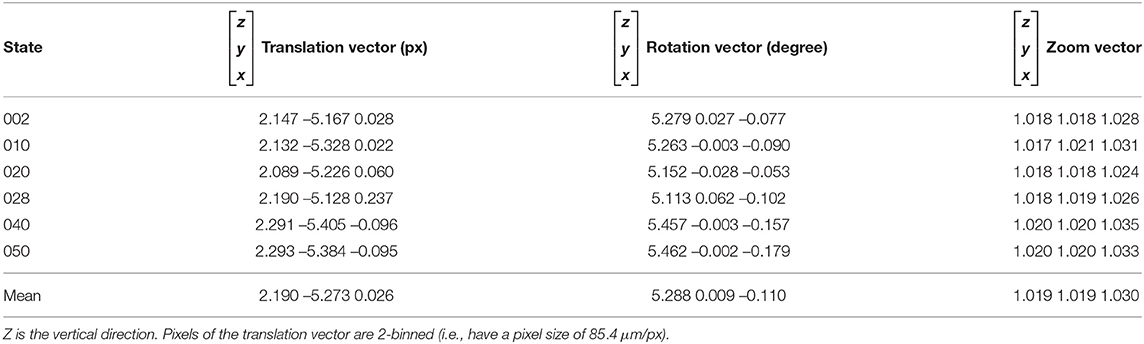
Table 1. Results of multiplicative polar decomposition of different Φ into translation, rotation, and “zoom” components to register μn fields onto μx fields for different imaged states.
The result of this application is now a vector-valued timeseries which is valuable and complex to plot. Figure 3 shows some selected horizontal slices from the registered volumes in state 002. The quality of the registration is apparent, as well as the complementarity of the fields measured with both modalities. Notably in the first slice, the denser aluminium attenuates the x-ray beam significantly whereas the membrane is hard to distinguish. The reverse is true for the neutron beam where the hydrogen-rich membrane attenuates enough to cause artefacts and where the aluminium is close to the background value for air.
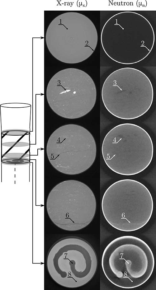
Figure 3. Selected horizontal slices through registered μx and μn fields in state 002, highlighting the different phases in the material. The greylevels shown are [0–42,000] for μx and [0–52,000] for μn. As per convention, dark values in the slices represent lower values. 1. Aluminium top cap, 2. Latex membrane, 3. “Dense” inclusions, 4. “Less dense” inclusions, 5. “Dry” crack, 6. Water-filled crack, 7. Pure water, 8. Aluminium bottom cap.
These complementary measurements are also useful for identifying different types of inclusions in the sample studied. Furthermore, the neutron tomographies allow the identification of dry and water-filled cracks. Table 2 shows a number of phases whose corresponding grey values have been identified by hand averaging over small homogeneous zones in the image. The table offers a numerical confirmation of the particular sensitivity of neutrons to water, which will be essential for the identification of the movements of water in this specimen. It is important to note that a small variation in the values of μx is observed throughout the timeseries, thus, a linear rescale of the values is applied to all images after 002, based on the grey values of air and water which should not vary in time. Considering air as the zero-intercept a linear correction is applied to all images such that the values of the air and the aluminium are always the same throughout the timeseries.
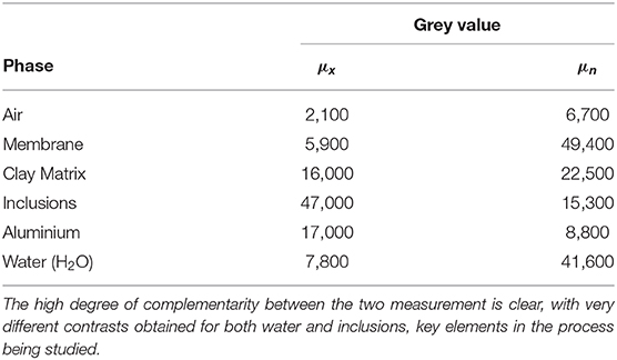
Table 2. Manually-measured average grey values of different phases visually present in μx and μn in state 002.
A powerful tool to look at the correspondence of greyvalues in these registered images is the joint histogram of μx and μn values. For two aligned voxelised volumes, the joint histogram is simply computed by discretising the greyvalues of μx and μn into bins, and for each voxel position in both volumes, adding 1 into the corresponding bin in μx and μn that two greylevels falls into. The result is a 2D space of discretised μx and μn values inside which counts are recorded. Large number of voxel pairs are expected to be found at the intersections of greylevels in Table 2. Figure 4 shows the joint histogram for state 002, with the full 16-bit image range discretised into 128 bins. In fact, this joint histogram (and the fitting of each relevant peak with a bivariate Gaussian distribution) is a fundamental part of the multimodal registration presented above.
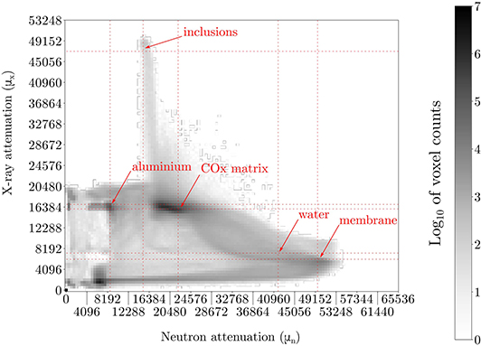
Figure 4. Joint histogram of state 002, count values are presented in a log10 scale. Intersecting values from Table 2 are highlighted.
The images acquired during the wetting process in this material are numerous, so a subselection has been selected in Figure 5, which shows the evolution of a slice normal to the crack initially present in the sample, which is labelled as “Dry” crack in Figure 3. Figure 5 also presents—in the black and white right column—the corresponding joint histograms for the entire volume of each pair. The changes in the joint histogram are rather subtle, however if attention is paid to the zone around the clay matrix, some changes can be observed.
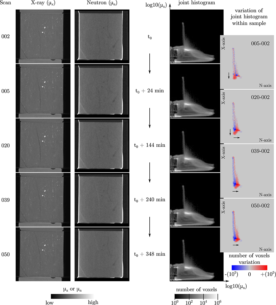
Figure 5. Vertical slices through registered μx and μn fields throughout the wetting experiment. Slice has been chosen to be normal to the main crack present since the beginning of the experiment in the specimen. As per Figure 3, the greylevels shown are [0–42,000] for μx and [0-52,000] for μn. As per convention, dark values in the slices represent lower values. Columns 3 and 4 represent the joint histograms of the pairs of images: column 3 is the entire joint histogram of the two images, with the counts being presented in log10. Column 4 represents a difference in counts (also in log10) from 002 on a cropped zone within the specimen.
For a better understanding of the evolution of the joint histograms, the difference between each time-step (005, 020, 039, 050) to the initial (002) has been calculated, indicating the increase of number of voxels in red and a decrease in blue (Figure 5). In addition, this difference of the joint histograms has been calculated on a cropped subvolume wholly within the sample, resulting in a range of values that cover a smaller area in the space of the joint greylevels. Similarly to Figure 4, the horizontal axis of these joint histograms corresponds the grey level values of the neutron images, while the vertical axis represents the grey level from x-rays, plotted in log10 scale.
As deduced from the incremental joint histograms, at the beginning (005–002), an increase of the number of voxels at the bottom of the vertical axis (x-ray axis) occurs in a location corresponding to the grey values of the “Dry” crack. This implies that between Scan 002 and Scan 005 an increase of the “quantity of Dry crack” is measured based on the amount of the corresponding grey level voxels from the x-ray images. Indeed, looking at the vertical slices, crack opening is well observed in the x-ray images—unlike the neutron ones.
In the following increment of joint histograms (020–002) crack opening is still observed—always along the vertical axis—however, an evolution along the horizontal axis (neutron axis) starts to appear around the same location. Increase of the grey values in the neutron images can be related to water appearance, an increase that becomes even more apparent in the following increments (039–002 and 050–002). When relating the observed evolution to the actual vertical slices, it can be confirmed that a clear water increase is depicted in the neutron image, with a filled-up crack (high attenuation). From then on, a continued increase in water penetrating the clay matrix is revealed from the last increment of joint histograms (050–002).
3.2. Displacement and Strain Field Measurements
In order to measure the deformation of the material with time, a local-DVC code is first used (the spam-ldic script available in spam, Andò et al., 2017). With this technique, a regularly-spaced grid of points is spread through the “reference” 3D image (in this case the x-ray scan of state 002). A cubic subvolume, centred on each grid point is extracted from the 3D image and a transformation Φ is sought for each point to minimise:
Here the Lucas and Kanade technique is used (Lucas and Kanade, 1981) with a deformation function (Grédiac and Hild, 2013; Tudisco et al., 2017). In this work, the x-ray volumes are used to measure the displacement, although in the future, the vector-valued (μx and μn) field could be used for the minimisation.
An initial time-saving step is the measurement of an overall Φ between the field of μx in state 002 and later states, which serves as an initial guess for the displacement of all points on the grid which will then be correlated. Figure 6 shows the progression of εzz, εradial, and εvol with progressive registration with state 002. These scalars are obtained by extracting the displacement gradient tensor from the measured Φ: the component εzz is directly read out, the volume change is computed as the determinant of the displacement gradient tensor, and is computed as per Wood (1990).
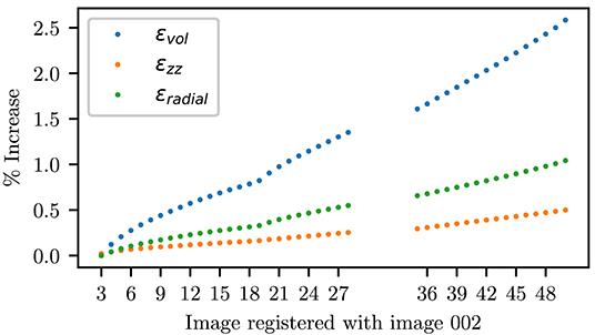
Figure 6. Vertical and volumetric deformations obtained from registrations (i.e., a correlation yielding a single Φ for the entire 3D volume) with μx fields with state 002. Each tomography takes 8 min.
Analysis of Figure 6 immediately reveals that there is indeed swelling occurring on average. The extent of swelling is significantly less than what was expected from the previous study (Stavropoulou et al., 2019)—which is likely explained by a higher initial water content in the sample studied here, together with its different shape, size, and a potential confinement applied by the membrane.
In order to look at swelling locally, a displacement field must be measured and strains computed. Of particular interest is to be able to compare local strains to changes in μn, which should indicate—all other things being the same—water arrival. In this work, displacement fields are measured with two different image correlation techniques, non-rigid local correlation and global correlation, both available in the spam toolkit.
The local displacement field is measured by defining a regular grid of measurement points with an equal spacing of 40 pixels (in non-binned images, which means 1.7 mm) in all directions. Each point is represented by a cuboid subvolume of greylevels centred on the point. The overall registration is then used as an initial guess for the displacement of each measurement point. The volumetric strain can either be extracted from the determinant of a locally-measured Φ as above, or by deriving the displacement gradient from the translation part of Φ from neighbouring measurement points. The first approach is extremely noisy, and cannot be used meaningfully given the relatively subtle volumetric strains that are trying be to captured. The second technique works well, however since measurement points are represented by subwindows and are used multiple times to measure strains, the physical space represented by a strain point is not direct. However, the displacement fields measured are of excellent quality, and are added to the data uploaded to Zenodo for a variety of subvolume sizes (see Data Availability Statement).
The lack of a direct interpretation of the physical subvolume represented by a strain measurement point in local DVC motivates the use of global DVC (Leclerc et al., 2011), where a continuous mesh is deformed to best match two images (to minimise η as above). In this case a cubic tetrahedral mesh of 360 × 160 × 160 pixels or 15.4 × 6.8 × 6.8 mm within the specimen is used. The edges are avoided since the current implementation of the technique has no mechanical regularisation and therefore problematic behaviour can occur on the edges. A characteristic size of tetrahedron of 80 pixels or 3.4 mm is found to give sufficiently low-noise in the strain computation1. The global convergence criterion is the norm of the displacement vector and for the correlations performed here, the criterion is slowly relaxed from 0.01 px for the early steps to 0.15 px for the later ones. The mesh generated contains 448 tetrahedra, on which strains are computed from the obtained nodal displacements. Figure 7 illustrates the quality of the measured global displacement field in the two penultimate increments of the images presented in Figure 5 (the correlations of the last two images 002–049 and 002–050 present two diverging points on the boundary). Furthermore, Figure 9 shows a part of the field measured.
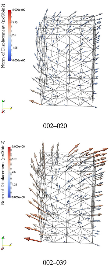
Figure 7. Displacement field as measured with Global DVC. The displacement at the nodes of the mesh is shown with vectors scaled up by 25×, and whose colour represents the norm of the vector. The mesh is shown in its reference state (i.e., in 002).
3.3. Measurement of Local Greyscale Variations
Given the ability to follow material points through time with the displacement fields described above, the variation of the measured fields (μx and μn) will now be discussed. Considering as an example the case of thermal expansion with no mass transfer, the expectation would be for the density of the material to reduce, and for both μx and μn to decrease proportionally to the change in density. In this experimental configuration however, it is likely that the swelling is caused by water interaction with the material. This hypothesis will be evaluated for the process being studied by looking at change of μx and μn inside each tetrahedron, compared to the expected change due to the measured volume change. The particular sensitivity of neutrons to water should reveal water entry into the clay matrix.
During fluid entry, two major phenomena will cause a variation in the absorption levels of x-rays and neutrons. On one hand, if the material swells, assuming (for now) mass conservation of the solid part, this implies that the mass density of the solid part will decrease, leading to a decrease in the level of attenuation. On the other hand, if the swelling is associated with an increase in the water content, then the presence of the additional fluid will modify the material's attenuation level (and may increase it if the attenuation coefficient of water is higher than the solid).
Considering that the infinitesimal volume can be decomposed into a solid part “s,” a free water part “wf,” an adsorbed water part “wa” and air “a,” the decomposition in the initial configuration (time 0) and the deformed configuration (time t) is (in the style of Coussy, 2007):
and
with
where J is the Jacobian of the transformation i.e., J ≈ 1 + εv. A number of hypotheses are made:
First it is assumed (common assumption in soil mechanics), that the volume of the solid skeleton does not change in time, leading to .
Furthermore, we assume that the density of free water is close to the density of adsorbed water, and consequently that the attenuation coefficients are the same: . This is supported by recent work at the nano-scale on the properties of adsorbed water, see Honorio et al. (2017) and Brochard (2019).
If we now consider a voxel (Ωvoxel = cst), each phase will contribute to the total attenuation through what we name here “partial attenuation” β and thus,
This assumes that the measured attenuation coefficient of the material is the result of a Gaussian mixture of the component attenuation coefficients. The partial attenuation of each phase is the attenuation of the phase weighted by the volume fraction of the phase as follows: where i is {s, w, a}.
In the case of a fully saturated sample, Ωa = 0 and thus,
In terms of solid partial attenuation, we have:
In terms of water partial attenuation, we have initially:
and at time t:
Injecting these expressions of β into Equation (5) at time t gives:
Finally, the change in attenuation will be:
For small strains, J ≈ 1 + εv, thus Equation (11) becomes,
This model indicates, in fine that the change in attenuation coefficient (for both x-ray and neutron tomographies) is a simple function of the volumetric strain and two easily measurable greyscale quantities. For x-ray tomography, μ0 is higher than the water absorption coefficient μw (as detailed in Table 2), meaning that swelling due to water uptake should induce a decrease of the global absorption coefficient. This is the reverse for neutron tomography, where μw coefficient is much higher than μ0 absorption coefficient, and so the swelling due to water uptake induce an increase of the global absorption coefficient.
Figure 8 presents two quantities plotted together:
x axis The volumetric strain measured locally (i.e., on the tetrahedra in the mesh discussed above) always taking image 002 as a reference. This measurement comes directly from the displacements of the mesh at the four nodes involving each tetrahedron.
y axis The change in greylevels Δμx and Δμn in each tetrahedron. This is computed as follows: All the voxels belonging to one tetrahedron are identified in the reference mesh, as well as in the deformed mesh. The mean value in the field corresponding to these voxels (which can be of different number in reference and deformed states) is recorded, and the difference is plotted here.
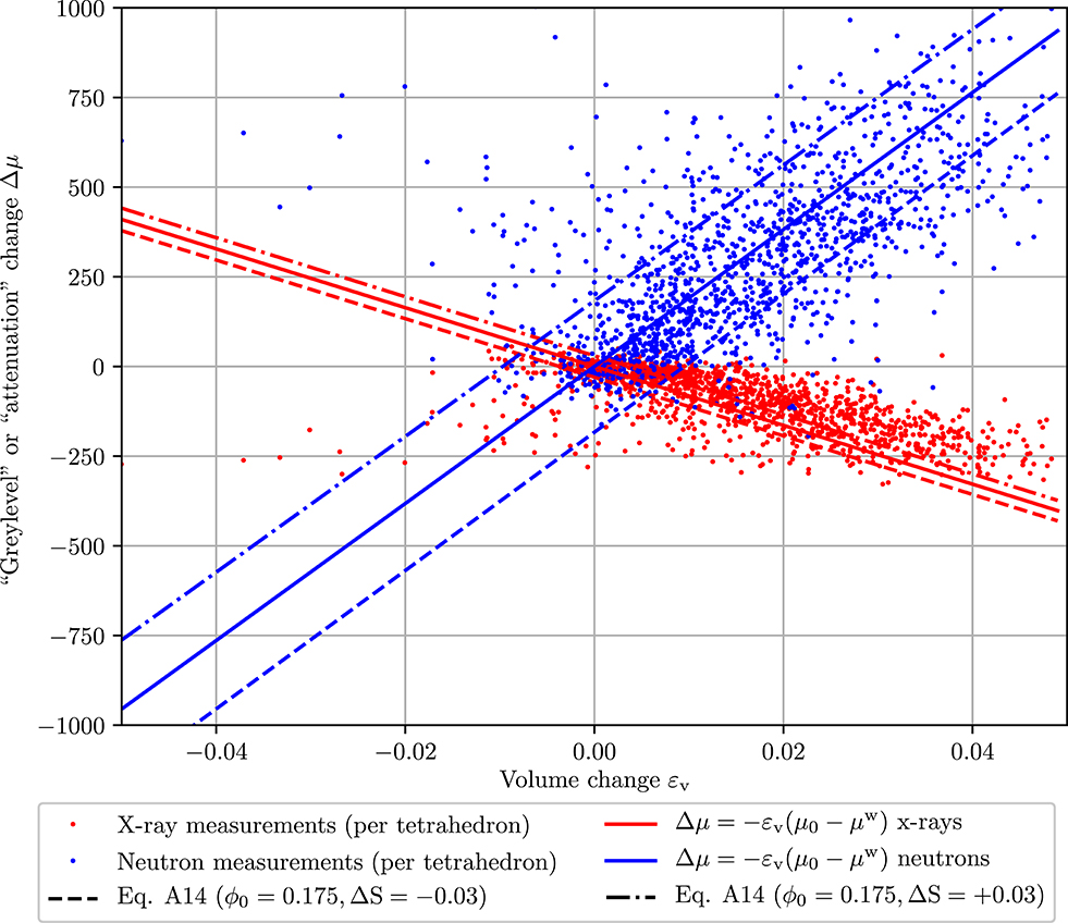
Figure 8. Data from Global DVC on increments 002-020, 002-039, and 002-0045. Volumetric strain of each tetrahedron plotted against the measured greylevel change in each tetrahedron. Expected changes of greylevel due only to the solid are added as per Equation (12). These scattered values for x-rays and neutrons are fitted with a linear regression separately.
Each point in the space presented represents the evolution (of size and greyscale) of one tetrahedron.
Figure 8 also includes the prediction as per Equation (12) in solid lines, taking μ0 as the mean measured value for the clay matrix from Table 2. The correspondence is quite satisfactory. The success of this simple model seems to indicate that the essential parts of the physics occurring have been captured adequately. Allowing a small change on the measured μ0 for x-rays an even better correspondence can be obtained (not shown).
A more sophisticated mathematical model is developed in the Appendix releasing the hypothesis that Ωa = 0 (thus allowing states of partial water saturation) and with the hypotheses that the volume of macro-voids does not change, and that swelling occurs only due to water adsorbed onto the clay aggregates (also valid above).
The upshot is that the change in greylevels can now be expressed as a function of volumetric strain (as before) and a new term linking the change of degree of saturation (ΔS) and the initial degree of open porosity (ϕ0):
This additional term allows the exploration of the influence of the change of degree of saturation during swelling. Taking ϕ0 as 17.5 % from Conil et al. (2018), ΔS can be evaluated, and lines for ±3 % are shown in Figure 8.
Returning to the fully saturated model, the spatial distribution of volumetric strain can be directly related to the increase of water (). Figure 9 presents a slice through half the sample colouring the tetrahedra in the analysed zone according to their volumetric strain for a few selected time intervals. In the first time increments an increase of strain at the bottom of the sample (which is in contact with the water supply) is visible, whereas toward the end of the experiment high values are recorded all over, with some indication of inhomogeneous levels of swelling.
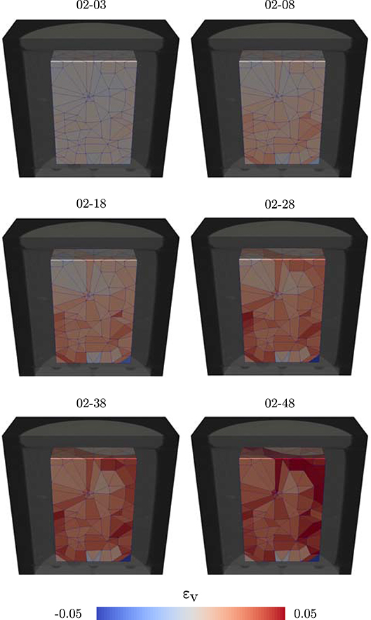
Figure 9. Semi-transparent rendering of the x-ray graylevels of specimen (state 002) with the mesh used for the total global correlation with tetrahedra colored by their volumetric strain. Using Equation (12) and its assumptions, the color bar for εv corresponds to .
4. Conclusion
This paper has presented a combined neutron and x-ray tomography analysis of water absorption behaviour in Callovo-Oxfordian claystone. These complementary imaging techniques are first of all registered into a common coordinate system using previous work, as well as a specially-developed graphical user interface to provide an initial guess. The resulting registered neutron and x-ray images of each state allow first of all a fine identification of the material phases present in the sample.
To characterise the gentle swelling process observed (around 2.5 % overall volumetric increase after almost 6 h) again the combination of x-rays and neutrons is exploited: local swelling is measured with Digital Volume Correlation thanks to the sharpness and low noise of the x-ray volumes (although it is mentioned that a correlation on the joint x-ray and neutron field could be developed in future). A mathematical model is developed for the expected local changes of greylevels in saturated conditions with all volume changes associated with water entry. The measurements are compared to this model with a good degree of correspondence, indicating that for this experiment on this sample, the model appears sufficient. This indicates that there are limited amounts of swelling due to chemical interactions for example.
This initial hydromechanical analysis (performed on a single sample) will obviously benefit from repetition, but a number of technical improvements to the analysis can also be envisioned.
• Anisotropic swelling–Instead of a scalar (εv) representing the change of volume of the material, the stretch tensor itself could be used to measure anisotropic parts of swelling related to the bedding known to affect this material.
• Taking into account microstructure–here the analysis has focused on the averaged local behaviour of the clay matrix. Further steps in the analysis could identify different types of inclusions known to be present (carbonates, quartz, pyrite) from the joint histograms, and relate a local degree of swelling to the presence of these aggregates.
• Taking into different initial states–further experiments are certainly necessarily, and of chief interest is to study different initial water contents as well as different stress states.
• Taking into account permeability/swelling times–The analysis as it stands implies a “time-free” relationship between water arrival and volumetric strain, whereas the characteristic times related to the very low permeability in the material may be interesting to include in the model, and which would explain long distance interactions through fluid pressure/suction.
Finally, a number of recommendations can be made for better estimations of the reconstructed attenuation coefficients:
1. Ensure that sufficient pure water is visible in a scan (on the neutron side in this case there are only 2 slices inside the spiral. Scanning a pure sample of water is also possible, but as far as neutron tomography is concerned, this must be a small cross-section to minimise the effects of scattering.
2. Given the importance that the mathematical model puts on the “physical” meaning of greyvalues, a long initial scan with lower noise provides a valuable reference for all μ values.
3. Selection of a less neutron-attenuating membrane material such as Teflon, or fluorinated silicons.
Data Availability Statement
The raw datasets collected on NeXT-Grenoble are available at http://doi.ill.fr/10.5291/ILL-DATA.UGA-42 – the experiment analysed is 03-3N5. Furthermore, a number of key outputs from this paper are available on Zenodo https://zenodo.org/record/3628018 with doi: 10.5281/zenodo.3628018.
• 01-volumes – Registered μx and μn fields at a pixel size of 85.4 μm/px – which is 2-binning for the x-ray volumes.
• 02-JH – Dynamic Joint histograms for all pairs of registered μx and μn fields calculated over the mask available in folder 01.
• 03-DVC – Results of registration, local Digital Volume Correlation with spam-ldic which describe a locally-measured Φ from scan 002 throughout the test for different half-window sizes, and Global DVC displacement fields.
Author Contributions
All authors listed have made a substantial, direct and intellectual contribution to the work, and approved it for publication.
Conflict of Interest
The authors declare that the research was conducted in the absence of any commercial or financial relationships that could be construed as a potential conflict of interest.
Acknowledgments
Laboratoire 3SR is part of the LabEx Tec 21 (Investissements d'Avenir–grant agreement n°ANR-11-LABX-0030).
Tom Arnaud is gratefully acknowledged for his central role in the programming of the graphical interface to the multimodal registration tool.
The high precision machinists SMGOP in Fontaine are kindly thanked for their contribution to the building of the experimental setup.
The ANDRA (French radioactive Waste Management Agency) is thanked for providing the claystone core used in this work.
The absorption model has been developed in the framework of the EJP EURAD (WP Hitec) – grant agreement 847593.
Footnote
1. ^This validation is performed by “zooming” μx 002 by 1.01 in all directions and correlating the original image with the zoomed version of itself. The application of this 3 % volumetric strain to the greylevels of μx is done through interpolation which reduces noise. Variance is additive, so the variance is measured in the original image, and the missing noise is added to the zoomed image.
References
Andò, E., Cailletaud, R., Roubin, E., Stamati, O., and the Spam Contributors (2017). spam: The Software for the Practical Analysis Of Materials. Available online at: https://ttk.gricad-pages.univ-grenoble-alpes.fr/spam/.
Andra, S. (2005). Dossier 2005 Argile: Synthesis: Evaluation of the Feasibility of a Geological Repository in an Argillaceous Formation, Meuse/Haute-Marne Site. Technical report.
Armand, G., Conil, N., Talandier, J., and Seyedi, D. M. (2017). Fundamental aspects of the hydromechanical behaviour of callovo-oxfordian claystone: from experimental studies to model calibration and validation. Comput. Geotech. 85, 277–286. doi: 10.1016/j.compgeo.2016.06.003
Bonin, B. (1998). Deep geological disposal in argillaceous formations: studies at the tournemire test site. J. Contam. Hydrol. 35, 315–330. doi: 10.1016/S0169-7722(98)00132-6
Bornert, M., Vales, F., Gharbi, H., and Nguyen Minh, D. (2010). Multiscale full-field strain measurements for micromechanical investigations of the hydromechanical behaviour of clayey rocks. Strain 46, 33–46. doi: 10.1111/j.1475-1305.2008.00590.x
Brochard, L. (2019). “Revisiting thermo-poro-mechanics to explain the anomalous thermal pressurization of water in clay,” in Joint GeoMech-M2UN workshop on Upscalling for Strategic Materials (Montpellier).
Chiang, W.-S., LaManna, J. M., Hussey, D. S., Jacobson, D. L., Liu, Y., Zhang, J., et al. (2018). Simultaneous neutron and x-ray imaging of 3D structure of organic matter and fracture in shales. Petrophysics 59, 153–161. doi: 10.30632/PJV59N2-2018A3
Chiarelli, A.-S., Ledesert, B., Sibai, M., Karami, M., and Hoteit, N. (2000). Influence of mineralogy and moisture content on plasticity and induced anisotropic damage of a claystone; application to nuclear waste disposals. Bull. Soc. Géol. 171, 621–627. doi: 10.2113/171.6.621
Conil, N., Talandier, J., Djizanne, H., de La Vaissière, R., Righini-Waz, C., Auvray, C., et al. (2018). How rock samples can be representative of in situ condition: a case study of callovo-oxfordian claystones. J. Rock Mech. Geotech. Eng. 10, 613–623. doi: 10.1016/j.jrmge.2018.02.004
Coussy, O. (2007). Revisiting the constitutive equations of unsaturated porous solids using a Lagrangian saturation concept. Int. J. Num. Anal. Methods Geomech. 31, 1675–1694. doi: 10.1002/nag.613
Delay, J., Lebon, P., and Rebours, H. (2010). Meuse/haute-marne centre: next steps towards a deep disposal facility. Int. J. Num. Anal. Methods Geomech. 2, 52–70. doi: 10.3724/SP.J.1235.2010.00052
Desbois, G., Höhne, N., Urai, J. L., Bésuelle, P., and Viggiani, G. (2017). Deformation in cemented mudrock (callovo-oxfordian clay) by microcracking, granular flow and phyllosilicate plasticity: insights from triaxial deformation, broad ion beam polishing and scanning electron microscopy. Solid Earth 8:291. doi: 10.5194/se-8-291-2017
DiStefano, V. H., Cheshire, M. C., McFarlane, J., Kolbus, L. M., Hale, R. E., Perfect, E., et al. (2017). Spontaneous imbibition of water and determination of effective contact angles in the eagle ford shale formation using neutron imaging. J. Earth Sci. 28, 874–887. doi: 10.1007/s12583-017-0801-1
Escoffier, S. (2002). Caractérisation expérimentale du comportement hydromécanique des argilites de Meuse/Haute-Marne (Ph.D. thesis). Institut National Polytechnique de Lorraine, Nancy, France.
Grédiac, M., and Hild, F. (2013). Full-Field Measurements and Identification in Solid Mechanics. London: Wiley Online Library.
Homand, F., Shao, J.-F., Giraud, A., Auvray, C., and Hoxha, D. (2006). Pétrofabrique et propriétés mécaniques des argilites. Comptes Rendus Geosci. 338, 882–891. doi: 10.1016/j.crte.2006.03.009
Honorio, T., Brochard, L., and Vandamme, M. (2017). Hydration phase diagram of clay particles from molecular simulations. Langmuir 33, 12766–12776. doi: 10.1021/acs.langmuir.7b03198
Leclerc, H., Périé, J.-N., Roux, S., and Hild, F. (2011). Voxel-scale digital volume correlation. Exp. Mech. 51, 479–490. doi: 10.1007/s11340-010-9407-6
Lenoir, N., Bornert, M., Desrues, J., Bésuelle, P., and Viggiani, G. (2007). Volumetric digital image correlation applied to x-ray microtomography images from triaxial compression tests on argillaceous rock. Strain 43, 193–205. doi: 10.1111/j.1475-1305.2007.00348.x
Lucas, B. D., and Kanade, T. (1981). “An iterative image registration technique with an application to stereo vision,” in Proceedings DARPA Image Understanding Workshop (Pittsburgh, PA), 121–130.
Montes, H., Duplay, J., Martinez, L., Escoffier, S., and Rousset, D. (2004). Structural modifications of callovo-oxfordian argillite under hydration/dehydration conditions. Appl. Clay Sci. 25, 187–194. doi: 10.1016/j.clay.2003.10.004
Robinet, J.-C., Sardini, P., Coelho, D., Parneix, J.-C., Prêt, D., Sammartino, S., et al. (2012). Effects of mineral distribution at mesoscopic scale on solute diffusion in a clay-rich rock: example of the callovo-oxfordian mudstone (Bure, France). Water Resour. Res. 48, 122–160. doi: 10.1029/2011WR011352
Roubin, E., Andò, E., and Roux, S. (2019). The colours of concrete as seen by x-rays and neutrons. Cement Concrete Composites 104:103336. doi: 10.1016/j.cemconcomp.2019.103336
Stavropoulou, E., Andò, E., Tengattini, A., Briffaut, M., Dufour, F., Atkins, D., et al. (2019). Liquid water uptake in unconfined callovo oxfordian clay-rock studied with neutron and x-ray imaging. Acta Geotech. 14, 19–33. doi: 10.1007/s11440-018-0639-4
Tengattini, A., Atkins, D., Giroud, B., Andò, E., Beaucour, J., and Viggiani, G. (2017). “Next-grenoble, a novel facility for neutron and x-ray tomography in grenoble,” in Proceedings ICTMS2017 (Lund).
Tengattini, A., Lenoir, N., Andò, E., Giroud, B., Atkins, D., Beaucour, J., et al. (2019). Next-Grenoble, the Neutron and X-ray Tomograph in Grenoble. ALERT Geomaterials, 47.
Tomasi, C., and Manduchi, R. (1998). “Bilateral filtering for gray and color images,” in Sixth international conference on computer vision (IEEE Cat. No. 98CH36271) (IEEE), 839–846.
Tudisco, E., Jailin, C., Mendoza, A., Tengattini, A., Andò, E., Hall, S. A., et al. (2017). An extension of digital volume correlation for multimodality image registration. Meas. Sci. Technol. 28:095401. doi: 10.1088/1361-6501/aa7b48
Wang, L., Bornert, M., Héripré, E., Chanchole, S., Pouya, A., and Halphen, B. (2015). Microscale insight into the influence of humidity on the mechanical behavior of mudstones. J. Geophys. Res. Solid Earth 120, 3173–3186. doi: 10.1002/2015JB011953
Wang, L., Bornert, M., Héripré, E., Yang, D., and Chanchole, S. (2014). Irreversible deformation and damage in argillaceous rocks induced by wetting/drying. J. Appl. Geophys. 107, 108–118. doi: 10.1016/j.jappgeo.2014.05.015
Wood, D. M. (1990). Soil Behaviour and Critical State Soil Mechanics. Cambridge: Cambridge University Press.
Yoo, T. S., Ackerman, M. J., Lorensen, W. E., Schroeder, W., Chalana, V., Aylward, S., et al. (2002). Engineering and algorithm design for an image processing api: a technical report on itk-the insight toolkit. Stud. Health Technol. Informatics 85, 586–592. doi: 10.3233/978-1-60750-929-5-586
Appendix – Theoretical Treatment of Partially Saturated Case
In order to relax the previous hypothesis of full saturation, a non-zero air volume must be allowed: Ωa ⩾ 0.
Introducing ϕ0 as the macro-porosity or “open” voids volume-fraction at time 0:
A hypothesis is however needed for the evolution of the voids volume with time during swelling; here we assume that the macro-porosity volume remains constant in time.
With S as the degree of saturation:
ΔS is then defined as the change in degree of saturation between time 0 and time t:
Moving onto partial attenuations, for the solid part nothing changes:
For the water part:
With the hypothesis that only the adsorbed water changes in volume during swelling:
and factoring by :
Now splitting St into S0 + ΔS:
Combining with finally yields:
Finally for the air:
The attenuation at time t, μt, can now be expressed as:
Subtracting μ0 in the same spirit as above:
In small strains:
Keywords: multimodal tomography, timeseries analysis, digital volume correlation, hydro-mechanics, callovo-oxfordian claystone
Citation: Stavropoulou E, Andò E, Roubin E, Lenoir N, Tengattini A, Briffaut M and Bésuelle P (2020) Dynamics of Water Absorption in Callovo-Oxfordian Claystone Revealed With Multimodal X-Ray and Neutron Tomography. Front. Earth Sci. 8:6. doi: 10.3389/feart.2020.00006
Received: 31 July 2019; Accepted: 15 February 2020;
Published: 11 March 2020.
Edited by:
Marco Voltolini, Lawrence Berkeley National Laboratory, United StatesReviewed by:
Harrison Lisabeth, Lawrence Berkeley National Laboratory, United StatesAnh Minh Tang, École des Ponts ParisTech (ENPC), France
Copyright © 2020 Stavropoulou, Andò, Roubin, Lenoir, Tengattini, Briffaut and Bésuelle. This is an open-access article distributed under the terms of the Creative Commons Attribution License (CC BY). The use, distribution or reproduction in other forums is permitted, provided the original author(s) and the copyright owner(s) are credited and that the original publication in this journal is cited, in accordance with accepted academic practice. No use, distribution or reproduction is permitted which does not comply with these terms.
*Correspondence: Pierre Bésuelle, cGllcnJlLmJlc3VlbGxlQDNzci1ncmVub2JsZS5mcg==