Geological Heterogeneity of Coastal Unconsolidated Groundwater Systems Worldwide and Its Influence on Offshore Fresh Groundwater Occurrence

Numerous coastal areas worldwide already experience fresh water shortages due to overexploitation and salt water intrusion. Future climate change and population growth will further intensify this threat in more areas in coming decades. Therefore, it is necessary to explore any potential fresh water source, such as offshore fresh groundwater, that could alleviate this fresh water shortage and provide valuable time for adaptation measures implementation and changes in water management strategies. Recent evidence suggests that a disproportionally large portion of human population living in coastal areas relies on groundwater resources stored in underlying unconsolidated groundwater systems. These systems are often very heterogeneous, combining numerous high permeability aquifers interlaid with low permeability aquitards with varying total thickness. This heterogeneity is a major control on the fresh groundwater volume and groundwater salinity distribution within such systems. Thus, the quantification of geological heterogeneity is often the limiting factor when estimating fresh groundwater volumes, both inland and offshore, along the global coastline. To overcome this obstacle, we combine conceptual geological models with available state-of-the-art global datasets to derive a set of geological heterogeneity parameter distributions quantifying geological heterogeneity of coastal unconsolidated groundwater systems (CUGSs) as formed over last 1 Ma. These are then used in an algorithm designed to build synthetic heterogenic parameterizations of CUGSs along the global coastline. These, in turn, provide key input for modeling variable-density groundwater flow and coupled salt transport to analyze changes in groundwater salinities and offshore fresh groundwater volume (OFGV). Such an analysis is performed over one full glacial–interglacial cycle (the last 0.13 Ma) to account for oscillating sea-level conditions and shifts in coast-line positions and salinity incursions. Our simulation results show a close match between the modeling scenarios and values presented by literature sources demonstrating the potential of the hereby presented methodology to be applied in similar future studies.

Introduction

Currently, more than two billion people live in the coastal areas worldwide (Ferguson and Gleeson, 2012) and are directly dependent on local fresh water resources. Aquifers bearing fresh groundwater are often tapped due to high water quality demands for domestic, industrial, and agricultural purposes and thus contribute to the energy and food security (Gleeson et al., 2015). In past decades, an increased pressure is observed on both shallow and deep (modern and fossil) inland fresh groundwater resources which results in depletion and quality deterioration (e.g., due to rising salinity), especially in arid regions (Custodio, 2002; Gleeson et al., 2017). These fragile fresh water sources are also threatened by natural hazards such as seawater-overwash events (Yang et al., 2013, 2018; Cardenas et al., 2015; Chui and Terry, 2015; Yu et al., 2016; Gingerich et al., 2017) and sea-level rise (Carretero et al., 2013; Rasmussen et al., 2013; Sefelnasr and Sherif, 2014; Mabrouk et al., 2018), further stressing the need to adjust water management strategies and find potential additional sources of fresh water. According to the latest IPCC report (Masson-Delmotte et al., 2018), the past decade has seen a record-breaking number of such natural disasters (seawater overwash events such as storm surges) while sea-level rise predictions are increasingly alarming (e.g., Pollard and Deconto, 2016). Furthermore, rapidly growing population numbers (e.g., United Nations, 2017) will lead to increased urbanization and consequently to coastal aquifer over-exploitation and lower groundwater recharge rates into the aquifers due to surface sealing (e.g., Custodio, 2002). Michael et al. (2017) stress the need to rapidly improve current water management strategies in coastal areas worldwide to adapt to the threats mentioned above.

Offshore fresh groundwater volumes (OFGVs) could act as an important additional fresh water resource in times with rising water stress in densely populated coastal areas (Cohen et al., 2010). A study by Post et al. (2013) shows that the OFGVs occurrence along the global coastline is higher than previously thought, while they can stretch even hundreds of kilometers offshore (Meisler et al., 1984; Edmunds and Milne, 2001). It is also important to note that large volumes of brackish groundwater can be found offshore as well. The OFGVs result from recharge that occurred in times of sea-level fall and low stands associated with the Pleistocene ice ages (e.g., Waelbroeck et al., 2002), notably prolonged and deep in the last 1 Ma (e.g., Pillans et al., 1998; Head and Gibbard, 2005), when the shelf groundwater systems interacted with surficial fresh water bodies like rivers and lakes. Additionally, a lower sea-level position also leads to higher groundwater gradient tilted toward the offshore domain. It can be assumed that the fresh groundwater flux coming from the landward direction is therefore increased and contributes to the OFGV creation. Sudden sea-level rise during glacial terminations produced low permeable aquitards deposited on top of the former coastal floodplains (Kooi and Groen, 2001; Pham et al., 2019). The sea-level rise led to deposition of shelf mud belts and estuarine-deltaic low-permeable deposits that rapidly trapped the formerly deposited fresh water. Inner and middle shelf regions went through these geomorphological cycles with each Pleistocene ice age (e.g., Hanebuth et al., 2002; Ehlers and Gibbard, 2004; Reijenstein et al., 2011; Cohen and Lobo, 2013). Such rapid inundating event due to sea-level rise and consequent trapping of OFGVs occurred between 17 and 7 ka BP and culminated during the Holocene (e.g., Smith et al., 2011; Lambeck et al., 2014). Thus, our main hypothesis is that OFGVs are formed by recharge during sea-level low stands and subsequently trapped by deposited low permeable sediments.

The above explained global effects of rapid sea-level rise leading to trapping of OFGVs suggests that such reserves are non-renewable on much shorter human-usage time scales (Post et al., 2013; Stone et al., 2019). However, a recent study by Michael et al. (2016) showed that large fresh groundwater fluxes (submarine groundwater discharge) can occur under certain conditions (linked to geological heterogeneity) and thus replenish the OFGVs. We do not attempt to determine the source of potentially found OFGVs in our study. Also, their vicinity to and intercalation with non-fresh shelf groundwater volumes of marine nature means that OFGVs are likely to gradually shrink due to natural salinization processes (namely, advection and hydrodynamic dispersion). Therefore, pumping these offshore fresh water reserves should not be considered as “mining” in the negative sense and could on the contrary even lead to reducing the current negative effects of onshore groundwater pumping (Kooi and Groen, 2001). However, the study by Yu and Michael (2019) found that offshore pumping could potentially impact the onshore land subsidence rates and submarine groundwater discharge depending on geological complexity. Hence, a need exists for better understanding of coastal geological heterogeneity when assessing OFGVs for potential exploitation, and to secure that such is not harmfully impacting hydrogeological conditions in the adjacent onshore.

The most recent OFGV discovery and quantification in the northeast U.S. Atlantic continental shelf has a magnitude comparable to the largest onshore aquifers (Gustafson et al., 2019). Other regions where OFGV was recently documented and studied are Malta, South Island of New Zealand (Micallef et al., 2018), and the Perth Basin in Australia (Morgan et al., 2018). Since a certain degree of salinization in such water bodies is to be expected, e.g., due to hydrodynamic dispersion, desalinization treatment would be necessary to make the extracted water from this source safe for human consumption (Gustafson et al., 2019). Tapping into the OFGV may not yet be needed in northeast United States, but it might play a significant role in regions already experiencing fresh water shortages and relying increasingly on desalinization. The latter brings about numerous environmental threats, the most urgent being generation of brine by-product that requires considerable economical and technical resources to be dealt with (Jones et al., 2019). These can be largely reduced by using fresh or slightly brackish water (i.e., OFGV) as feedwater to desalination plants and thus cutting down the brine output and energy costs (Ghaffour et al., 2013). Moreover, OFGV could supply low-cost water in areas with offshore oil production activities (Yu and Michael, 2019). This adds to the urgency of better understanding and quantifying the OFGV occurrence before these can be successfully mined for human consumption.

Recent analytical and SEAWAT (Langevin et al., 2008) modeling studies underline the importance of heterogenic geological conditions (mainly presence and extension of aquitards) on potential OFGV occurrence (Van Engelen et al., 2018; Knight et al., 2018; Morgan et al., 2018; Solórzano-Rivas and Werner, 2018), turning away from earlier simulations embedding homogeneous geological conditions (Ranjan et al., 2009; Michael et al., 2013; Werner et al., 2013; Ketabchi et al., 2016) and moving toward more complex heterogeneous subsurface representation (e.g., Michael et al., 2016; Zamrsky et al., 2018; Thomas et al., 2019).

The main objective of this study is an estimation of the geologically heterogeneous structure of regional coastal unconsolidated groundwater systems (CUGSs) in order to arrive at an estimate of the OFGVs in these systems. Performing this estimation leads to schematizations in which we experimentally vary additional uncertain properties. These are limited to the ratio between thicknesses of permeable and low permeable layers (aquifers resp. aquitards), cross-sectional geometry of aquitards and within that aquitard discontinuity and degree of consolidation. When using the schematizations to simulate trapping of OFGVs and assess their potential sizes, we assume that the distribution of low permeable layers has had the largest influence on OFGVs. This is the outcome of sediment delivery to and dispersal over the shelf while changing according to sea-level oscillations between repeated low and high stands (OFGVs being recharged during low stands, trapped and stored during high stands).

A major constraint to the hydrogeological heterogeneity estimations is a lack of direct observational information suitable for use at the global scale. Another issue is, besides the practical problem of uneven coverage, the non-uniformity and proprietary restrictions on what data are there (geological and hydrological; seismic swaths; cores and wells). A further fundamental problem is that data acquired in the few sectors of shelves for which data are reasonably disclosed (references above), cannot be simply assumed to also be representative for the shelves rest of the world. In practice, this means that attempts to estimate shelf architectural heterogeneity and their OFGV contents have to rely on synthetic hydrogeological representations that are built on the global data (bathymetry, mapping the size of shelves) and geological insights (age of shelves, relations with the continents that fed them, understanding of sea-level cyclicity, and sediment routing to the deep sea) that are available, and the geological-history shared versus the geographically diverse aspects herein. Such provides a baseline synthetic geohydrological representation of the shelf subsurface of use in independent OFGV modeling (this study), also functioning as a primer that alternative approaches starting from direct data (i.e., non-synthetic shelf geomodeling) can compare to.

Based on such insights and rationale, we populate and re-aggregate a global shelf map with relevant geological information, use it to draw synthetic geological sections with explicitly simulated architectural heterogeneity. Subsequently, we use these as input for variable-density groundwater flow and coupled salt transport models. In such a way, it is possible to estimate the volumes of fresh groundwater located both the inland and offshore domains and asses the influence of varying geological conditions on these volumes. We demonstrate the workflow to quantify OFGVs for seven selected coastal regions. In SEAWAT (Langevin et al., 2008) model simulations, we consider a full glacial–interglacial cycle in order to correctly capture OFGV temporal dynamics under changing sea levels and also test our hypothesis that such volumes can be preserved over a time scale of tens of thousands of years. We also include a future prediction of OFGV shrinking due to salinization but do not take into account any sea-level rise predictions.

The decision to limit the aim to CUGSs only stems from high pressure on current and future fresh water availability in these areas compared to sedimentary rock groundwater systems (see also Zamrsky et al., 2018). For similar reasons, we excluded CUGS in Arctic and Antarctic regions and focus on shelf regions of the tropics and temperate latitudes (including those with shelf sediment delivery affected by glaciations during low stands). Including sedimentary rock groundwater systems (including karstic recharge systems) would require the implementation of very different geological complexity concepts which are beyond the scope of this paper.

Materials and Methods

General Approach

In this study, we first focus on geological heterogeneity estimation of the unconsolidated continental shelf systems. The information gathered is then fed into a synthetic heterogenic parameterization algorithm to create multiple random geological approximations of these systems. Then, as the third and final step, SEAWAT (Langevin et al., 2008) modeling procedures are designed to investigate the potential presence of OFGV in a set of chosen coastal regions. To achieve that, the globe is divided into regions connecting a continental shelve to a river basin that supplies its sediments. These regions are typified based on their geological character (sediment supply, sediment type, subsidence rate) using global datasets. Next, a methodology is devised to systematically generate average representative profiles (ARPs) of coastal regions that aggregate various regional characteristics (e.g., topography, geological input, groundwater recharge estimation, etc.). Thus, the ARP approach serves as a tool to estimate the mean groundwater concentration profile in each individual coastal region. This estimation is carried out by running for each ARP a large set of SEAWAT (Langevin et al., 2008) models simulating variable-density groundwater flow and coupled salt transport to quantify the probable range of fresh water occurrence in both coastal (inland) and continental shelf (offshore) domains, given the local geological uncertainty. Expecting that large model runtimes might be a potential bottleneck due to high spatial resolutions over very long simulation times (>150 ka), we investigate whether a reduced number of geological realizations per ARP will provide sufficiently accurate results compared to a larger random set. This approach is tested on a selected set of coastal segmentation and related catchments (COSCAT) regions and corresponding ARPs and later compared to past studies dealing with OFGV assessments.

CUGSs Regionalization Using COSCAT River Basin and Continental Shelf Divisions

The COSCAT (Meybeck et al., 2006) and margins and catchments segmentation (MARCAT, Laruelle et al., 2013) divisions carve the land of the globe into large river basin-based regions (COSCATs) acting as sediment sources connected to the corresponding sediment depositional areas (sinks) located along the continental shelf (MARCATs). Coupling between these two datasets is carried out to match the continental shelf domain segments to the corresponding COSCAT region. This division into COSCAT regional areas is the cornerstone of our study. It provides the spatial dimensions of the shelf terrains as major sink areas, and allows to connect these areas to the continental source catchment areas for which size, elevation, and climatology are specified within our study. Various state-of-the art global datasets are collected to characterize the geological conditions of these regional areas (see Table 1). These datasets are then combined through a set of equations to determine continental shelf architecture (interlayering aquifer and aquitard layers). A detailed description is provided in the Supplementary Material.

TABLE 1

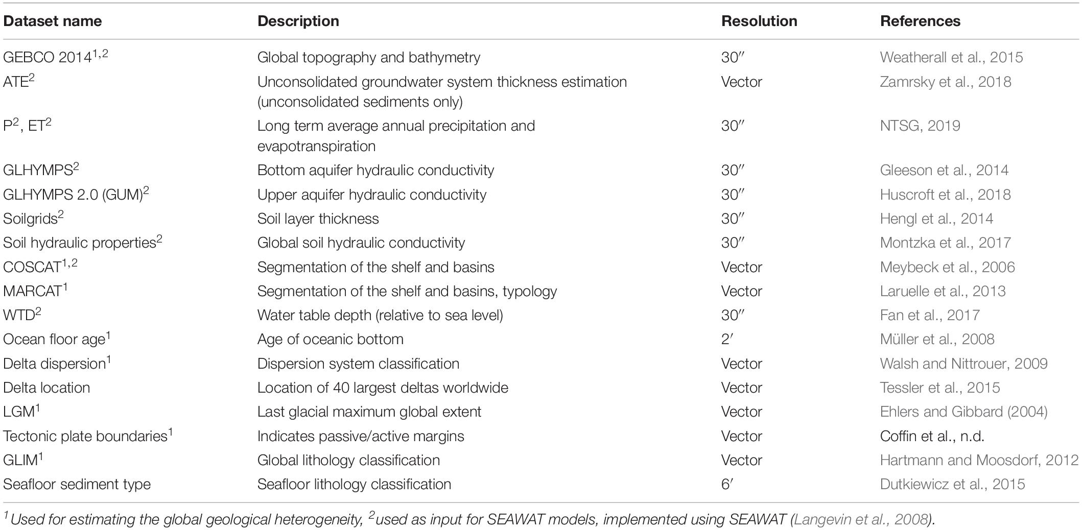
Table 1. Global datasets collected and used as input.

The resulting estimated continental shelf architectures are quantified by parameterizing the geological heterogeneity conditions per COSCAT region and its corresponding continental shelf domain segment (see section “Global Geological Heterogeneity Parameterization”). Table 1 lists the full suite of datasets used to generate and populate the coastal profile SEAWAT models. Extracting individual datasets along the cross-section perpendicular to the coast and running through individual coastal points located along the global coastline is performed in the same fashion as in Zamrsky et al. (2018). The distance between each of the individual coastal profiles is 5 km while the cross-section points along each profile are 0.5 km apart. This is a far greater resolution than the number of COSCAT regions that can stretch over hundreds or even thousands of kilometers of coastline. This scale difference, however, serves to include a realistic amount of variation in continental shelf architecture.

Not included in the geological parameterization are polar shelf regions (e.g., around Antarctica), partly due to missing input datasets, and partly due to low population density and the presence of permafrost. However, subpolar shelf regions affected by major glaciation (e.g., around North America and Scandinavia) are included. Finally, regions without any CUGS are omitted from the SEAWAT modeling step.

Global Geological Heterogeneity Parameterization

This section provides only a general summary of the methodology to derive parameters quantifying geological heterogeneity of the continental shelf architecture (see detailed explanation in the Supplementary Material). To do that, a number of global datasets were used as inputs into various conceptual schematizations gathered from literature translated into equations (see Table 1). Among the main natural forces taken into account are the past sea-level oscillations that heavily influenced the sedimentation conditions over the past one million years (last 10 glacial–interglacial cycles). Sediment layers deposited during this time period constitute the bulk of CUGS worldwide. It is also necessary to mention that our focus is only limited to passive tectonic plate margins. These are generally older and more extensive than active tectonic plate margins and thus dominating the global continental shelf domain.

Continental shelf architecture is mainly characterized by assessing the accommodation and sedimentation properties for each COSCAT region including factors influencing that ratio. The sedimentation/accommodation ratio Y (−) is derived as follows (Eq. 1):

$$Y=\frac{Sedimentation}{Accommodation}=\frac{q_s^{*}{M}^{*}D}{R}(1)$$

where $q_s\left[\frac{m}{Myr}\right]$ sediment flux (supply) into the continental shelf domain;

M[−] sand/mud composition ratio;

D[−] sediment dispersion modifier;

$R\left[\frac{m}{Myr}\right]$ long-term net subsidence (thermal term + compaction term).

The outcome for each of these individual factors and their influence on continental shelf architecture is shown in Figure 1. Sediment supply (q_s) magnitude mainly affects the thickness of individual sediment layers and is estimated based on Syvitski et al. (2003): WHYMAP. The sediment type forming these layers is defined by the M (sand/mud composition) ratio, based on inner continental shelf sample collection (e.g., Hayes, 1966) with modifications for the composition during glacial times (e.g., Nam et al., 1995). The factor influences the presence, thickness, and composition of aquitard layers within the CUGS (next sections). The sediment dispersion modifier Ddetermines the fraction of sediment that is deposited on the continental shelf compared to the continental slope. Lastly, the long-term net continental shelf subsidence factor R plays a crucial role in assessing the continental shelf architecture. The thermal subsidence term is dependent on oceanic crustal age (Karner and Watts, 1982). The compaction term (e.g., Reynolds et al., 1991) is calculated making use of the q_s and D parameters. A more detailed description of the global geological heterogeneity parameterization is provided in the Supplementary Material.

FIGURE 1

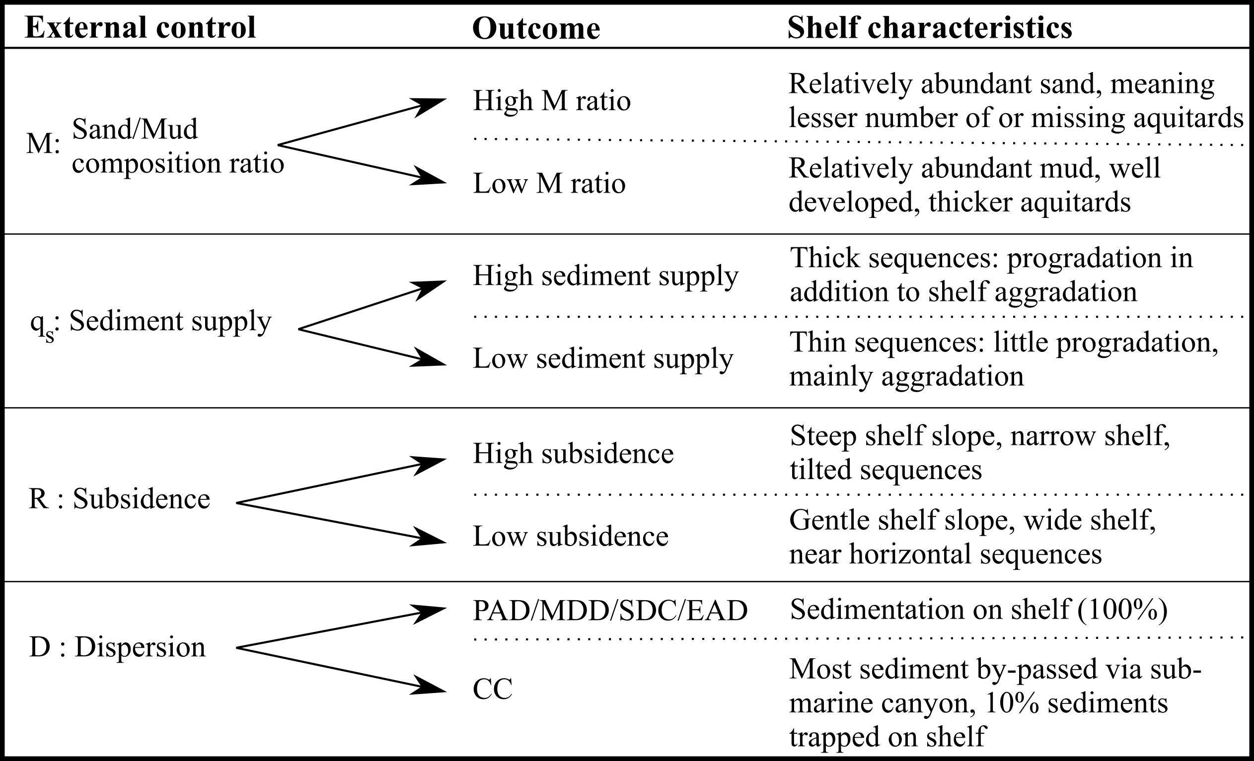
Figure 1. Hydrogeological summary variables for COSCAT/MARCAT shelf regions. The sediment dispersion modifier D is 1 for all but one of Walsh and Nittrouer (2009)’s shelf categories (EAD: estuarine accumulation dominated; PAD: proximal accumulation dominated; SDC: subaqueous delta clinoforms; MDD: marine dispersal dominated). It is set to 0.1 for those shelved captured by major submarine canyon systems.

Both the integrate Y parameter and its constituent variables R, D, M, and q_s are used as input parameters for the geological heterogeneity algorithm for the ARPs. Two additional geological parameters are used in that algorithm. First, we define a parameter to characterize preservational discontinuities in the shelf architecture as produced by alternating deposition and erosion over multiple glacial–interglacial cycles. To determine this parameter, we used the information available from surficial lithology descriptions describing the discontinuities of sediment layers deposited during the Holocene era. To overcome insufficient knowledge on older sediment layers and their discontinuities, we simply reproduce the same parameter value stochastically over these layers. The parameter is called aquitard patchiness factor, defined to capture the vertical and horizontal continuity of low permeable aquitard layers in the geological heterogeneity algorithm. Areas with high Y values (leading to coastal erosion) also have a high aquitard patchiness value. Second, to define the sediment type of the upper sediment layer in the offshore domain, we use the offshore lithology classification which is based on the dataset generated by Dutkiewicz et al. (2015) (see Table 1). Multiple lithological classes are merged into two large groups (permeable and non-permeable).

Average Representative Profiles (ARPs) Concept

As mentioned above, constructing ARPs is used as a concept to depict a mean profile for a selected set of seven COSCAT regions considered in this study. The averaging process involves parameters determining coastal prism dimensions such as the mean topographic and bathymetric profiles together with the inland and offshore extent of the ARP (Weatherall et al., 2015), and the mean aquifer (groundwater system) thickness estimation (ATE) at the coastline (Zamrsky et al., 2018) for each selected COSCAT region. Since COSCAT regions spread over areas with similar climatic conditions, the averaged difference between long-term net annual precipitation and evapotranspiration (NTSG, 2019) is taken as the groundwater recharge estimate. Lastly, the regional geological characteristics described in section “Global Geological Heterogeneity Parameterization” are derived for individual COSCAT regions and therefore can directly be used as input for estimating the average thickness of the CUGSs.

Coastal Profiles and Types

The individual coastal profiles perpendicular to the coastline are evenly spaced along the coastline where unconsolidated sediments are found. Parameter values derived from the datasets listed in Table 1 are extracted for each individual coastal profile by a Python toolbox. Subsequently, these profiles are aggregated into the ARP per COSCAT region as described above in section “Average Representative Profiles (ARP) Concept.” Figure 2 shows a schematized COSCAT region with individual coastal profiles positioned perpendicular to the coastline.

FIGURE 2

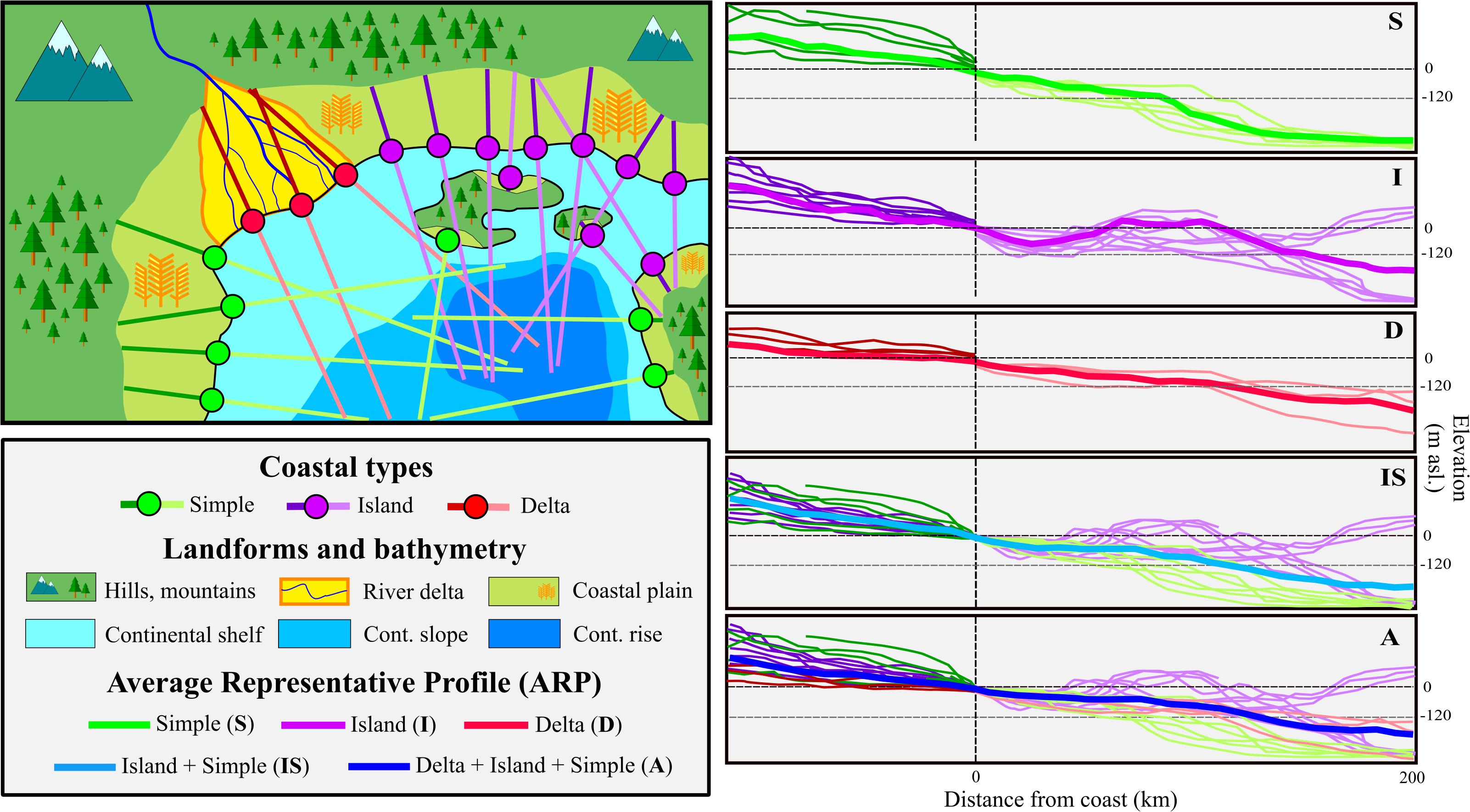
Figure 2. Average representative profile (ARP) and coastal type schematization. The bathymetry classes are based on elevation and slope of the ocean floor. Pinet (2003) defines the three main bathymetry classes based on depth below sea level and topographical slope. Continental shelf is the shallow and relatively flat part of the ocean floor with its depth below sea level not exceeding 120 m below sea level (assumed to be the lowest sea level throughout a glacial cycle, see Figure 6). At the edge of the continental shelf, there is an abrupt change in slope which marks the beginning of the continental slope. At the end of continental slope is the continental rise that is defined by lower slope and large depths (generally deeper than 3000 m below sea level).

The inland areas are classified based on the GLIM lithological classification (Hartmann and Moosdorf, 2012) and elevation (Weatherall et al., 2015). These databases split the hinterland into higher elevated and mostly rocky hilly or mountainous areas and the low-lying coastal plain consisting of unconsolidated sediments. The border between these two classes also corresponds to the landward boundary position in the 2D SEAWAT models. Since deltaic areas are assumed to have generally thicker unconsolidated groundwater systems (Zamrsky et al., 2018), a special attention is paid to the largest deltaic systems worldwide (Tessler et al., 2015) creating a separate inland class on its own. The offshore domain is divided into three classes based on two criteria: (a) the ocean floor depth below sea level and (b) the bathymetry slope. These criteria are used to determine the position of the continental shelf edge (CSE) and foot of continental slope (FOS) points (Figure 3) using the algorithm presented by Wu et al. (2017).

FIGURE 3

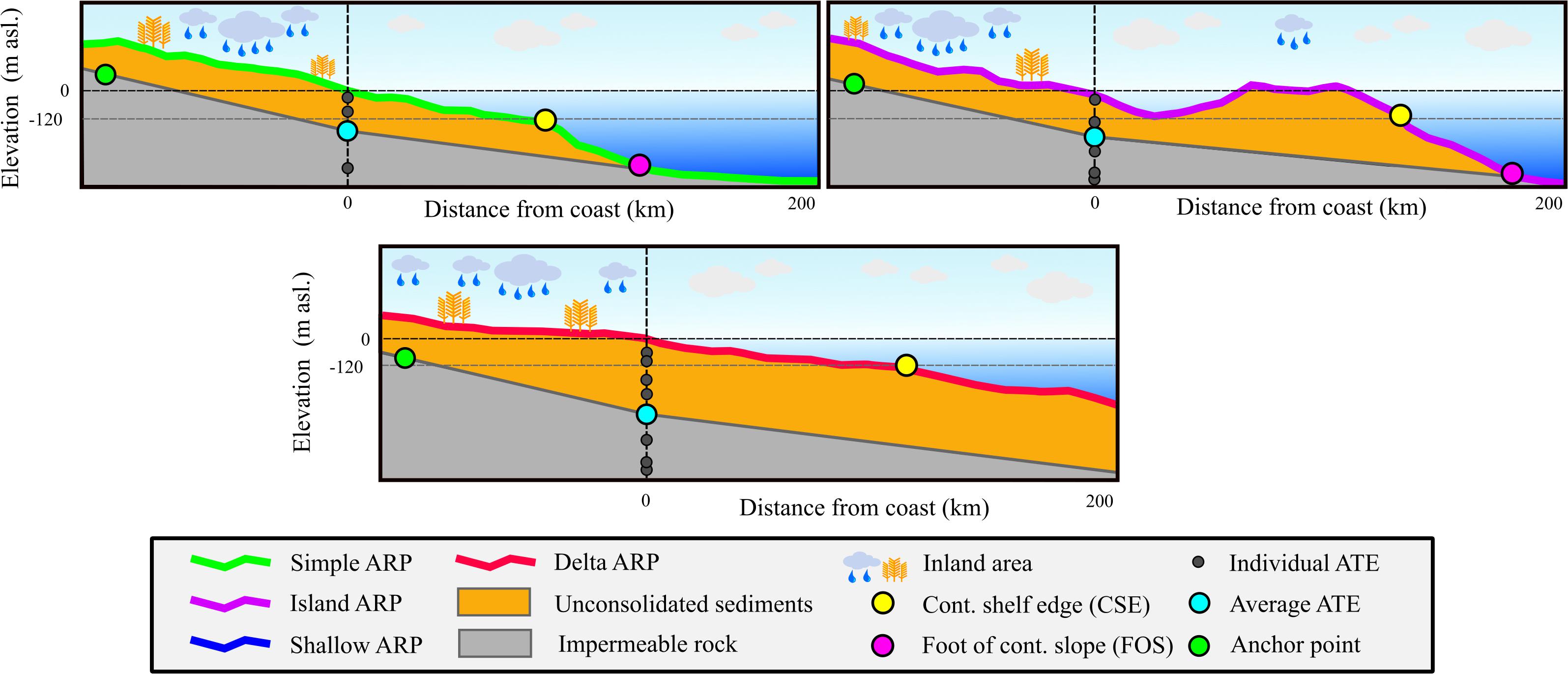
Figure 3. Defining the subsurface extent of average representative profiles (ARP)s: the foot of continental slope (FOS) and the continental shelf edge (CSE) are based on Wu et al. (2017) and the average aquifer thickness estimation (ATE) is established from Zamrsky et al. (2018).

Figure 2 also shows a coastal type classification that is defined by topographic and bathymetric criteria. When the coastal profiles have a clearly distinguished inland and offshore domain, they are classified as “Simple (S)” profiles. However, in quite a few cases, there can be a clearly detectable island (or barrier island) area present in the coastal profile and the profile is then classified as “Island (I).” Coastal profiles that fall within the areas marked as large deltas by Tessler et al. (2015) fall into the “Delta (D)” ARP class. Combining the profiles belonging to each of these coastal types leads to the formation of the ARPs per COSCAT region for each of the three coastal types. It is possible that combining coastal types can lead to an ARP that captures the characteristics of these coastal types. This can happen when the “Island (I)” ARP—after combining all the profiles—has no island in the offshore domain anymore and can therefore be merged with “Simple (S)” coastal type ARP, classifying it as an “Island + Simple (IS)” ARP (see Figure 2). Additionally, if the “delta” ARP shows similar topographical shape and coastal aquifer thickness, all three coastal types are merged, classifying it as a “Delta + Island + Simple (A)” ARP.

Creating Synthetic Heterogenic Parameterization of Coastal Unconsolidated Groundwater Systems (CUGSs)

After determining the model domains’ upper topographic and bathymetric limits, the next step is to define the depth of the impermeable bottom boundary. Using the average ATE value at the coastline and the thickness at the anchor point location (Zamrsky et al., 2018), a simple straight line is drawn between these two points, as shown in Figure 3. In the offshore domain, the bottom boundary is determined as a straight line between the average ATE point and the FOS. However, in cases where the FOS point is not found (e.g., the continental shelf domain stretches further offshore than 200 km), the bottom boundary is set to follow the average slope of the ARP’s bathymetric profile (see Figure 3) [“Delta (D)” ARP].

To fill the domain between the upper and bottom cross-section boundaries, an algorithm is designed to create a synthetic heterogenic CUGS. This geological heterogeneity algorithm uses as input the datasets listed in Table 1 and the geological parameters described in section “Global Geological Heterogeneity Parameterization.” It is assumed that during periods with high eustatic sea level (high stands comparable to current sea level), finer sediments are deposited both at the usually low-lying coastal plain and at the continental shelf. The properties of the top layer are determined using the SOILGRIDS and GUM datasets (see Table 1) in the inland domain of the ARP, and the offshore lithology dataset to establish the properties of the top layer in the offshore domain. Lower permeability of this top layer leads to slower infiltration of saline water into the CUGS and thus preservation of OFGVs (Post et al., 2013).

The form and structure of the offshore domain of the CUGS is determined by the sediment flux and sand/mud composition ratio parameters as described in section “Global Geological Heterogeneity Parameterization.” In systems with high sediment fluxes, the deposition of new sediment layers stretches further offshore and generally covers previously deposited layers. This leads to a forward protruding of CSE points as shown in Figure 4. Opposite to that, when the sediment flux is low, there is not enough sediment volume to cover the whole extent of older sediment layers and therefore there are no protruding CSE points. The sand/mud composition ratio is used to establish the aquifer and aquitard layer fractions in the whole CUGS. The total sand and mud fractions are then split into the desired number of aquifer and aquitard layers, respectively.

FIGURE 4

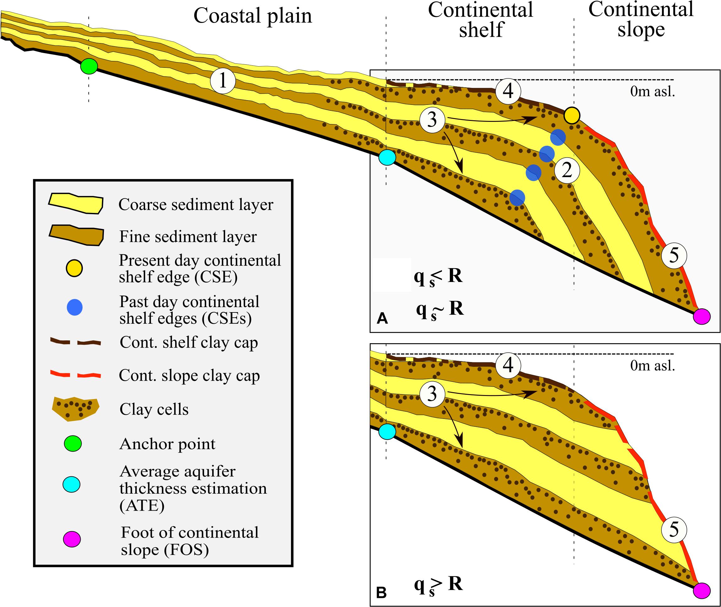
Figure 4. Conceptual schematization showing the process of translating the geological information and parameter values into a synthetic heterogenic CUGS profile. (1) The total number of high stand (coarser sediments/aquifers) and low stand (finer sediments/aquitards) layer pairs is determined on sediment sand/mud composition ratio R specified in section “Global Geological Heterogeneity Parameterization.” (2) The offshore layers shape is based on the sediment flux parameter value q_s; in this example, the value is “high” meaning that the sediment supply is so high that the shelf edge is being pushed further away from the coastline (A). In the opposite cases, the individual sediment layers are stacked on top of each other without fully over topping the lower layers (B). (3) Assuming that during maximum high stand sea levels mostly very fine sediments are deposited (e.g., as during Holocene sea-level transgression; Oude Essink et al., 2010) both inland and offshore (due to low river gradient) individual clay layers (represented by model cells) are inserted into the larger fine sediment layers. A so-called stacking factor is applied to determine how close these model cells containing clay are placed relative to the top of the fine sediment layer. (4) A clay cap layer is potentially placed on top of the ocean floor depending on the main sediment type as provided by Dutkiewicz et al. (2015). (5) Same as in (4) but in the continental slope area.

A so-called stacking factor is applied to determine the clay cell location within the aquitard. Varying it allows us to test the influence of aquitard leakiness in groundwater salinity simulations. A higher value of the stacking factor means higher probability of low permeable (e.g., clay) model cells toward the top of the aquitard that in turn leads to increased groundwater flow confinement. Lithologically, this resembles the fining upward sequence that is typically observed toward the top of low stand fluvial depositional systems (e.g., Bridge, 2009; Miall, 2014) and at the base of transgressive to high sea-level stand coastal deposits (e.g., Cattaneo and Steel, 2003). The overall proportion of clay cells in the aquitard is made to equal the parameter M as specified per COSCAT region in section “Global Geological Heterogeneity Parameterization”; the remainder is fine sediment based on the GLHYMPS data set (Table 1 and below). Presumably, the aquitard layers are formed and buried over the half glacial-interglacial cycle from low stand to high stand, such as lastly between 20 and 7 ka BP. To what degree the aquitard is preserved spatially, however, is determined after deposition and the architectural outcome of that is captured by applying the aforementioned aquitard patchiness factor (section “Global Geological Heterogeneity Parameterization”). Doing so builds conduits between aquifers, short circuiting the aquitards. These conduits are created randomly in the aquitard layers by removing an amount of low permeable cells corresponding to the aquitard patchiness factor and thus simulating the coastal erosion process. In such a way, we are able to create links between permeable aquifer layers and increase their connectivity which presumably has a large influence on groundwater flow patterns in CUGSs. The geological heterogeneity algorithm outcomes thus mimic the hydrogeological properties of the modeled domain. The process of creating this synthetic heterogenic CUGS is further illustrated in Figure 4.

SEAWAT Modeling

The computer code SEAWAT (Langevin et al., 2008) is used to simulate variable-density groundwater flow and coupled salt transport for the corresponding coastal type ARPs found in each selected COSCAT region. It is highly probable that in some parts of the world, large OFGVs were formed during low sea levels tens of thousands of years ago, when shelf floors were exposed during the Last Glacial Maximum (26.5 to 19 ka BP), and/or when riverine discharge increased during the termination of the Last Glacial (19 to 8 ka BP; also considering long periodic variations in monsoonal strength)—both facilitating increased fresh water recharge. For such reasons (see also: Post et al., 2013), the timescale considered in this study stretches beyond one full glacial–interglacial cycle to determine not only the current situation but also the temporal dynamics of these regional groundwater systems. The average OFGV (and its standard deviation) is estimated for the selected set of COSCAT regions and its corresponding coastal type ARPs under varying geological conditions. This set consists of seven COSCAT regions (see Figure 5), some of them with multiple coastal type ARPs (amounting to nine in total), where offshore fresh groundwater presence was documented by Post et al. (2013). This also serves as an additional validation procedure to gauge the fit of our modeling results. Two different modeling concepts are developed leading to a total number of 1116 SEAWAT model simulation runs (124 per ARP). In the SEAWAT models, the offshore extent is limited to 200 km, to keep model runtimes reasonable. All these simulations are performed on the Dutch HPC (high performance computing) cluster Cartesius facilitated by the SURFsara services.

FIGURE 5

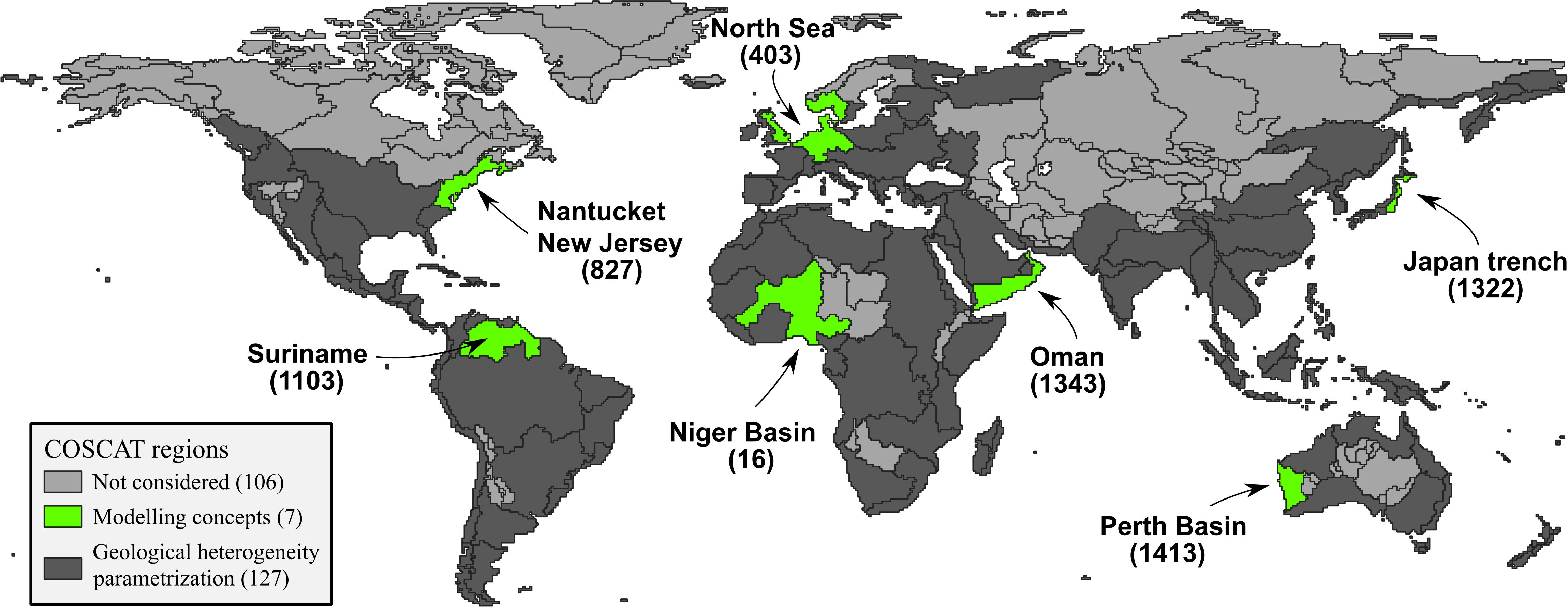
Figure 5. COSCAT regions selected for comparison of the two modeling concepts and the geological heterogeneity parameterization study. Northern arctic and inland COSCAT regions are not considered for this study. COSCAT region names (in brackets) correspond to areas with proven or highly possible presence of offshore fresh groundwater reserves (Post et al., 2013).

Hydrogeological Properties

The geological heterogeneity algorithm described in section “Creating Synthetic Heterogenic Parameterization of Coastal Unconsolidated Groundwater Systems (CUGS)” specifies the location of sediment layers deposited during past high and low sea-level stands. Hengl et al. (2014) provide a global thickness estimation dataset of the sediment layer (unconsolidated) presumably deposited during the last low sea-level stand. In our study, it is used to define the thickness of the upper most unconsolidated sediment layer in the model domain. The original GLHYMPS (Gleeson et al., 2014) and GUM (Huscroft et al., 2018) datasets define the overall hydraulic conductivity of the unconsolidated sediments. GLHYMPS shows values on average approximately one order of magnitude lower than that of the upper unconsolidated sediment layer (GUM). Since aquitard layers are usually deposited during high sea-level stands and have generally low permeability (i.e., low hydraulic conductivity values), they are assigned the GLHYMPS values. The opposite is the case for more permeable aquifer layers that are deposited during the low sea levels and are therefore linked to the GUM datasets.

Unfortunately, the exact information about the number of preserved aquifer–aquitard layer combinations for each selected COSCAT and their thickness is missing and thus needs to be approximated. We use the sand/mud ratio (see section “Global Geological Heterogeneity Parameterization”) to determine the fractions of aquitard and aquifer sediment layers deposited over a single full glacial–interglacial cycle. Subsequently, the number of aquifer–aquitard layer combinations is randomly assigned (see Figure 4). In a similar fashion, thickness of each aquifer–aquitard layer is also randomly determined until the whole total CUGS thickness is filled up. The upper most sediment layer thickness is determined based on Hengl et al. (2014) and hydraulic conductivity properties derived from the GUM dataset (Huscroft et al., 2018). This results in creating an approximate geological profile for the selected set of COSCAT regions and the corresponding ARPs. The exact aquitard position within the CUGS is also unknown and is therefore parameterized to start at a random distance (positive or negative) from the current coastline. In such a way, it is possible to examine the effects of the aquitard layer position on the estimated groundwater salinity profile.

The aquifer and aquitard layers are differentiated in the SEAWAT models via varying hydraulic conductivity values provided by the GUM and GLHYMPS datasets, respectively (see Table 1). These hydraulic conductivity values are extracted along each individual cross-section at equidistant points as in Zamrsky et al. (2018) and then combined into a single group (per sediment layer type) for each COSCAT region to draw realizations from. A lognormal distribution for both the GUM and GLHYMPS values is then created for each group and COSCAT region. A chosen value from these lognormal distributions is then assigned to each model cell in the model domain depending on the sediment layer type (aquifer or aquitard) allocated to the model cell as explained in section “Creating Synthetic Heterogenic Parameterization of Coastal Unconsolidated Groundwater Systems (CUGSs).” To simulate lower permeability of these aquitard layers, clay cells are then synthetically inserted into aquitard layers. Hydraulic conductivity values for clay cells are selected randomly (using Python randomization tools) and vary between 0.01 and 0.0001 m/day. This allows us to create a characteristic representation of regional hydrogeological conditions based on available state of the art global datasets.

Boundary Conditions of the SEAWAT Models

The bottom of the active model domain is assumed to be impermeable and is therefore set to a no-flow boundary. In the offshore domain, the upper most model cells are assigned a general head boundary (GHB) with concentration of sea water and sea-level head elevation. The extent of the offshore domain changes with sea-level fluctuations and the GHB extent is adjusted accordingly. Sea water GHB cells are also assigned to all model cells in the last offshore model column (in vertical direction) in cases where the FOS is not found and the offshore model domain extent is limited to 200 km. A water divide in the inland domain is determined using the ARPs topographical profile as described in section “Coastal Profiles and Types.” At this water divide, all the model cells are assigned a GHB with freshwater concentration and head elevation equal to the water table depth (relative to sea level).

A simple top system is used to enable groundwater recharge through the model cells located on top of the inland model domain whose extent shifts according to the sea-level fluctuations (as the GHB extent explained above). The groundwater recharge rate is calculated as the difference of annual average precipitation and annual average evapotranspiration (see Table 1) and is applied to the first active model cells of the inland areas of the model domain. Groundwater recharge is limited to a maximum rate taken as equal to the hydraulic conductivity of the cells the recharge is applied to.

Modeling Stress Periods and Sea-Level Fluctuations

Grant et al. (2012) approximated the global eustatic sea-level variations over the last glacial–interglacial cycle. This time span covers more than one full glacial–interglacial cycle that usually spans over around 125 ka based on the time elapsed between two maximum sea-level high stands. Our main hypothesis is that OFGVs are stored during the sea-level low stands covering the largest time span of the full glacial–interglacial cycle (see Figure 6). Paleo fresh groundwater recharge from precipitation spanning across the area corresponding to current continental shelf leads to deposition of these OFGVs (Post et al., 2013). Therefore, the last maximum sea-level high stand (125 ka BP) is considered as starting sea-level position for the numerical groundwater flow models. Figure 6 shows the temporal division within the modeling approach of SEAWAT: the so-called stress periods (SPs), being time intervals during which the inputs for the model remain constant. SPs are used to simulate fluctuating sea-level values and stretching over fixed time periods. Since sea-level drop represents a much larger part of the glacial–interglacial period and rate of sea-level change is also much slower than that corresponding to sea-level rise, the sea-level drop SPs are longer than sea-level rise SPs (5 and 2 ka, respectively). In this way, it is ensured that the sea-level fluctuation effect on groundwater flow and saline concentration dynamics are captured with enough detail.

FIGURE 6

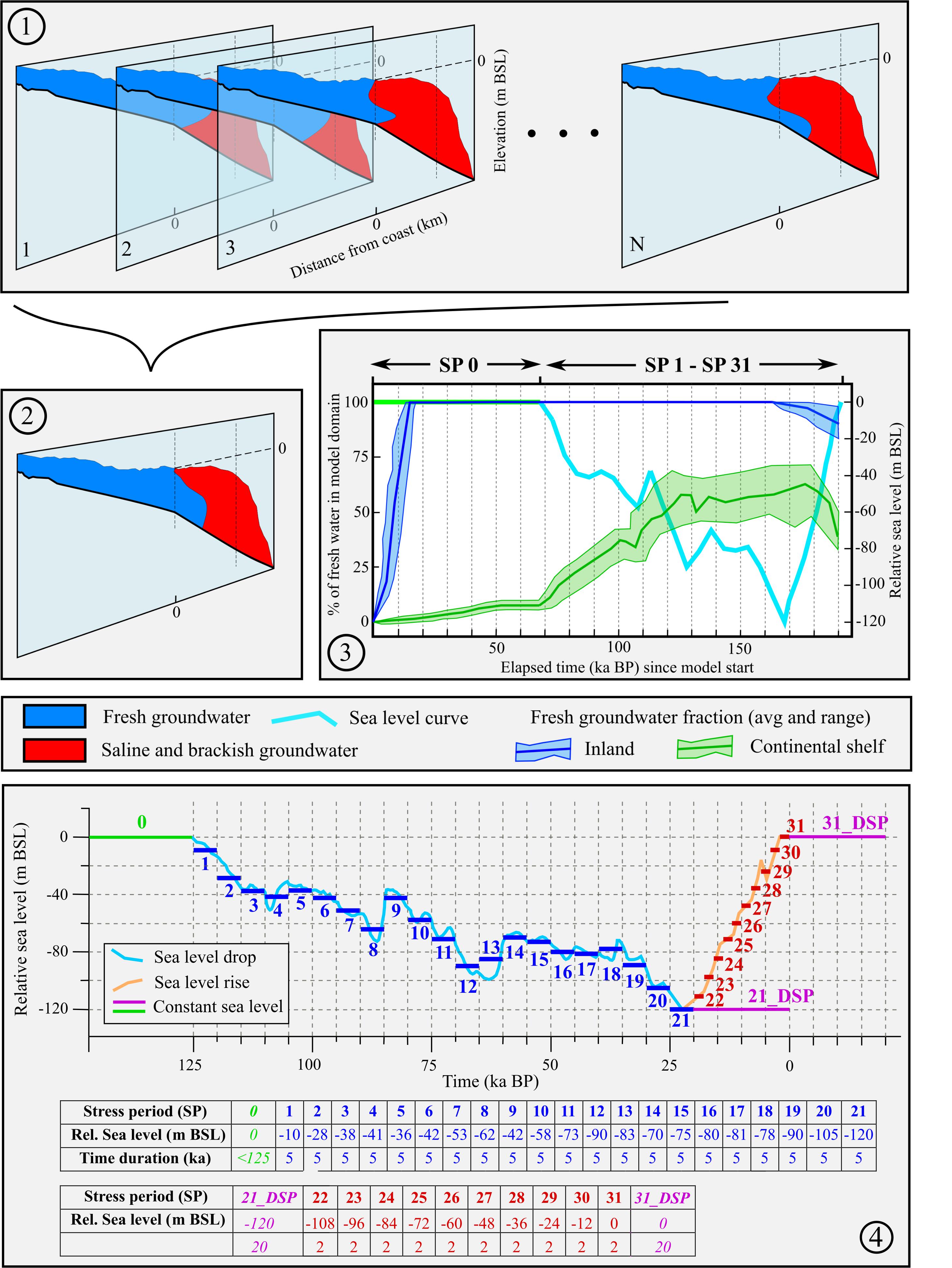
Figure 6. Combining all SEAWAT models per COSCAT region into an average presentation: (1) a number of N generated SEAWAT models (with different synthetic heterogenic CUGS and other model input parameters, see Table 2), each with a different groundwater salinity distribution. The fresh groundwater fractions (FGFs) are measure in both the inland (first 10 km inland from the present coastline) and the continental shelf (stretch from present coastline to continental shelf edge) areas; (2) all model outputs at all time steps are then averaged into an aggregated average profile; (3) graph showing the average fresh groundwater fraction and the range of fresh groundwater fraction across all individual SEAWAT models (overall minimum and maximum value) through time with varying sea levels that are shown in (4) stress periods (SP) with corresponding sea levels (m BSL) relative to current situation and their time duration in thousands of years. In the graph, the sea levels as a function of the past 125 ka (light blue and orange lines) are derived from Grant et al. (2012). The upper table shows stress periods with generally decreasing sea-level trend (blue horizontal segments in the graph) while the lower table corresponds to a time period of comparatively fast sea-level rise during the past 20 ka (red horizontal segments in the graph). So-called dynamic SPs (DSPs) are also implemented to study the groundwater systems dynamics in the selected COSCAT regions. Green line is implemented in the SEAWAT models to simulate the initial salinity profile (saline initial condition only) and is set to last no more than 125 ka (equal to one full glacial cycle); 21_DSP (20-0 ka BP) is set up to investigate the system inertia at the absolute sea-level low stand, while in 31_DSP (0–20 ka), we investigate the system inertia and in the future 20 ka with sea level kept at current level (0 m BSL).

TABLE 2

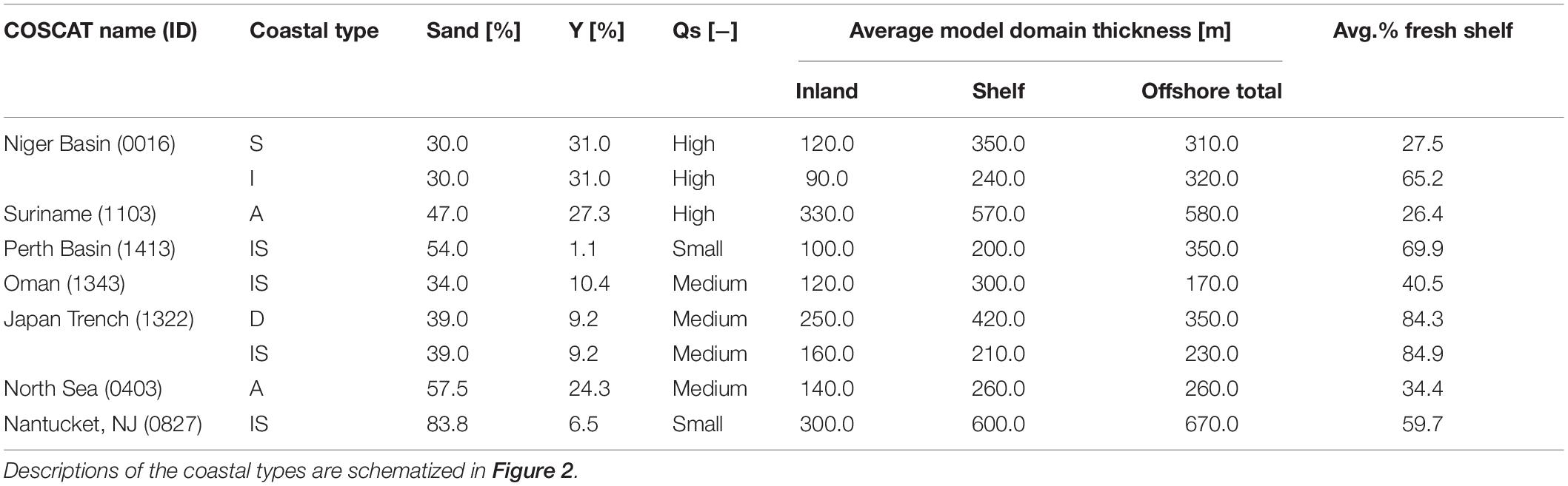
Table 2. Global geological heterogeneity parameter estimation for the seven selected sample COSCAT regions (see Figure 5).

The groundwater flow models are initially set to run for time duration of maximum one full glacial–interglacial cycle (125 ka) with the sea-level boundary set to 0 m bsl. (called the “saline” initial condition) [see Figure 6 (SP0)]. This approach is adopted to estimate starting groundwater salinity condition before simulating the full glacial–interglacial cycle with fluctuating sea level (SP1 to SP31). It also serves as a benchmark that is later compared to groundwater salinity of the individual SEAWAT models at absolute sea-level low and high stands (SP 21_DSP and SP 31_DSP, respectively). In such a way, we can assess the so-called system inertia of a groundwater salinity profile per selected COSCAT region. The system inertia per SP is defined here as the rate of OFGV change (% of total volume) in time during SP 21_DSP and SP 31_DSP. This allows us to gain insight into the assumed non-renewability of the OFGV. The SP 21_DSP SP is 20 ka long and represents a scenario with sea level kept at the absolute low stand (-120 m BSL). Groundwater salinity evolution during this SP is used to evaluate the maximum OFGV (if achieved within the SPs duration) present in the model domain. On top, it demonstrates whether the SEAWAT model of that specific ARP has achieved equilibrium of the groundwater salinity (see section “Convergence Criteria”). In a similar fashion, the system inertia while maintaining constant sea-level high stand (SP 31_DSP) is used to assess the change in estimated OFGVs in future 20 ka from the current condition (end of SP31) (we do not include sea-level rise scenarios into our analysis).

In certain ARPs, we observe that the bathymetry elevation is higher than the lowest sea level considered during the sea-level fluctuation simulation (-120 m BSL). A different approach needs to be implemented for such areas with shallow ocean floor (i.e., COSCAT 403_A) since they were flooded by sea water only recently (some tens of thousands ka BP). In such cases, the whole domain is set to fresh water (0.5 g TDS/L) initial salinity concentration, in contrast with the regular ARP where the initial groundwater salinity is saline groundwater. Only one SP with a constant sea level (0 m bsl.) is simulated given that the sea-level rise curve is very steep in the simulated time period. To assess the current OFGV in such a case, the lowest elevation of the ocean floor in the model domain is compared to the sea-level curve showed in Figure 6. The time elapsed between the corresponding SP and sea-level value and present day is then the time step at which the current OFGV is estimated. From that moment on, with the constant sea-level value (0 m BSL), the SEAWAT model simulation is extended for another 20 ka to assess the future evolution of the salinity concentration profile. This SP corresponds to the SP 31_DSP explained above.

Model Input Parameters

As described in sections “Hydrogeological Properties” and “Boundary Conditions of the SEAWAT Models,” multiple parameter types and values such as groundwater recharge rates and geologic composition are COSCAT region specific. However, some model settings are kept constant throughout this study and applied to all SEAWAT models. The finite difference solver is chosen for simulating salt transport, while using standard values for porosity, hydrodynamic dispersion parameters, based on other regional SEAWAT modeling studies (Ketabchi et al., 2014; Morgan et al., 2018; Mahmoodzadeh and Karamouz, 2019). The chosen grid resolution of 100 m wide and 10 m thick model cells is in accord with other previously published similar scale SEAWAT models (Cobaner et al., 2012; Michael et al., 2016; Huang and Chiu, 2018). A summary of the parameter values applied to all SEAWAT models is presented in the Supplementary Material.

Convergence Criteria

Two different types of convergence criteria are distinguished in this study. First, numerical convergence criterions for head and water budget (SEAWAT parameters “hclose” and “rclose,” see Supplementary Material) are defined to terminate a SEAWAT model simulation in case these convergence criteria are met. Note that since the total number of SEAWAT models is rather high (1116), some ARPs span over a large area (more than 200 km) and a complex geological system is implemented, it can happen that some SEAWAT models do not meet this criterion within the defined time span of one full glacial–interglacial cycle (125 ka) and individual SPs. One of the reasons why this numerical convergence is not achieved is potential head or concentration value oscillation in an individual model cell.

The second convergence criterion type is set up for this study to evaluate the change in groundwater salinity in the model domain over an SP of 1000 years; as to assess the system inertia we need to know when the groundwater salinity distribution has reached its dynamic equilibrium. The SP is further divided into 10 time periods of 100 years delimiting the time points at which groundwater salinity (and groundwater head) profiles are extracted. Next, the difference between two consecutive time steps is computed, both in absolute volumes of fresh water (model cells with fresh groundwater concentration count) and in the maximum absolute change in concentration (and head elevation) across the whole model domain of the ARP. The model is marked as converged if the maximum absolute change in both groundwater salinity and head is lower than 0.05 g TDS/L and 0.05 m, respectively. In cases when this condition is not satisfied, assuming mainly due to numerical oscillations in head or salinity, the secondary convergence criterion is examined since the changes in the groundwater salinity distribution over the whole model domain can be negligible. If the change in fresh groundwater volume is lower than 300 m³ per stretched meter, taking into account porosity (0.3) and total volume of one model cell (1000 m³) over the 1000-year long SP, the secondary convergence criterion is said to be reached. If either of these two criterions is reached, the current SP simulation is terminated and the next one is started. Combining these two criterions allows us to potentially save computation times when at least on is reached. Also, it assures the certainty of model simulation results by measuring the changes throughout the model simulation in groundwater concentration and heads.

Comparison of Two Modeling Concepts to Estimate OFGVs Under Geological Uncertainty

Two concepts of modeling and estimating OGVs under geological uncertainty are tested and compared to examine if it is possible to estimate OFGVs using only extreme geological heterogeneity parameter values [parameter extremes (PE)] compared to results of completely randomized Monte Carlo (MC) approach. The underlying reason for comparison is to save computation time considering that the large number of model cells, the long integration times, and the high total number of SEAWAT model simulations all leading to high model runtimes. The geological parameters whose value are varied across SEAWAT model simulations of both concepts are the aquifer–aquitard layer combinations, clay layer stacking factor, clay layer start, and offshore clay cap thickness (exact values provided in the Supplementary Material). In the first concept only, the PE combinations are used as input to the geological heterogeneity algorithm (see sections “Creating Synthetic Heterogenic Parameterization of Coastal Unconsolidated Groundwater Systems (CUGSs)” and “Hydrogeological Properties”) leading to a total 24 SEAWAT model simulations. The second modeling concept randomly selects a value within each parameter’s boundary values and creates a randomized MC parameterization set of 100 SEAWAT model simulations.

The total OFGV V_total (km³) is calculated as:

$$V_{total}=S{B}^{*}{D}_{shelf}^{*}{L}_{coast}^{*}{\frac{FG{F}_{mean}}{100}}^{*}p$$

where SB represents the CSE distance from the coastline (km), D_shelf is the average sediment thickness in the continental shelf domain (km), L_coast is the length of the given coastal (ARP) type along the COSCATs coastline (km), FGF_mean is the mean estimated fresh groundwater fraction (FGF) for the COSCAT region (%), and p is the effective porosity (−). The FGF_mean value is determined by averaging the fraction of fresh groundwater cells in the shelf domain as simulated by all individual SEAWAT models for each selected COSCAT region. The FGF is thus calculated as the total number of model cells with fresh groundwater concentration over the total amount of model cells in the shelf zone. Dividing the total estimated volume V_total by the coastal length L_coast allows for calculating the OFGV per kilometer of coastline as V_stretch = V_total/L_coast.

The two concepts are tested on the average estimated OFGV in the inland and offshore domains. The averaging process leading to analysis schematization of the final modeling result is shown in Figure 6, and displays the total average and range of the FGFs through time with varying sea levels. This comparison is performed for the selected set of seven COSCAT regions (resulting in nine ARPs) where offshore fresh groundwater presence was proven by Post et al. (2013) (see Figure 5). This also serves as an additional validation procedure to gauge the fit of our modeling results.

Results

Characteristics of Regional CUGS

Global Geological Heterogeneity Parameterization

The overall results for each individual geological heterogeneity parameter simulated as part of the global geological heterogeneity parameterization are shown in Figure 7. Quantitative estimations for seven selected sample COSCAT regions (total of nine ARPs) are provided in Table 2. A closer look at Figure 7 reveals that a large majority of global continental shelves is either aggrading (represented by a medium aquitard patchiness value) or forced regressive (high aquitard patchiness value). As explained in section “Global Geological Heterogeneity Parameterization,” this has to do with the sedimentation/accommodation ratio (Y). Cases where accommodation is larger than sediment supply occur mainly in the arctic shelves or in areas with no large rivers. Conversely, continental shelves in regions with high sediment supply via a large river and low subduction rate tend to have a high sedimentation/accommodation ratio value.

FIGURE 7

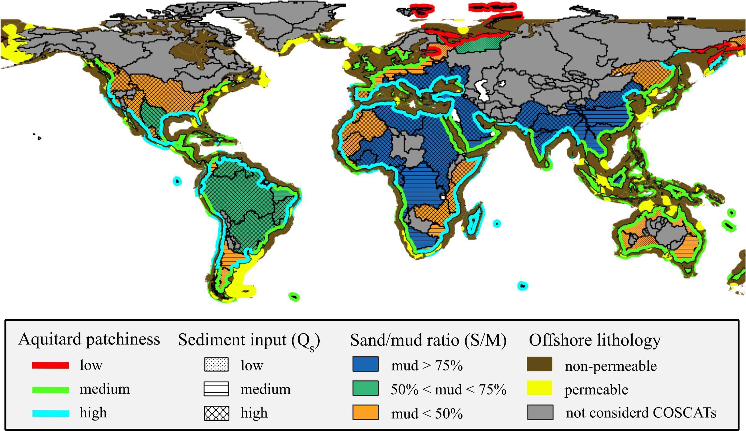
Figure 7. Geological heterogeneity parameterization results for COSCAT regions with CUGS present.

Regions with high sediment supply into the continental shelf can be characterized by a large hinterland area with high relief and/or high temperatures. These attributes increase the chances of progradation, aggradation, and thick strata deposition over the coastal plain and continental shelf domains. Such conditions can be found in, e.g., the Mississippi River delta, Amazon River delta, Yellow River delta, the North Sea, the Black Sea to just name a few. Similarly, to the sedimentation/accommodation ratio, the opposite conditions (small hinterland area, low relief, and/or low temperatures) lead to small sediment supply rates which in turn cause low chances of progradation, aggradation, and thick strata deposition (e.g., most of Australia).

The sand/mud composition ratio provides an insight into the potential presence of thick and numerous aquitards interlaying the aquifers. Most temperate and arid areas show high sand/mud composition ratio values while tropical regions or regions at active tectonic margin tend to have low sand/mud composition ratio values, as can be observed in Figure 7. In the offshore domain, most continental shelves and slopes are covered by non-permeable sediments and only a scattered set of areas worldwide is overlaid by permeable sandy sediments; this is assumed to increase the possibility for OFGV occurrence.

Synthetic Heterogenic Coastal Unsaturated Groundwater Systems (CUGSs)

Figure 8 shows a set of synthetic heterogenic CUGSs created using the geological parameters described above. Sediment layer progradation is observed in COSCAT region 1103_A (Suriname, high sediment flux) and is recognizable by preservation of past CSEs and change of the sediment layer slope in the offshore domain (Groen et al., 2000; Kooi and Groen, 2003). On the contrary, in areas with low sediment supply such as COSCAT 1413_IS (Perth Basin), the progradation effect is absent and individual sediment layers have constant slope over the whole offshore domain.

FIGURE 8

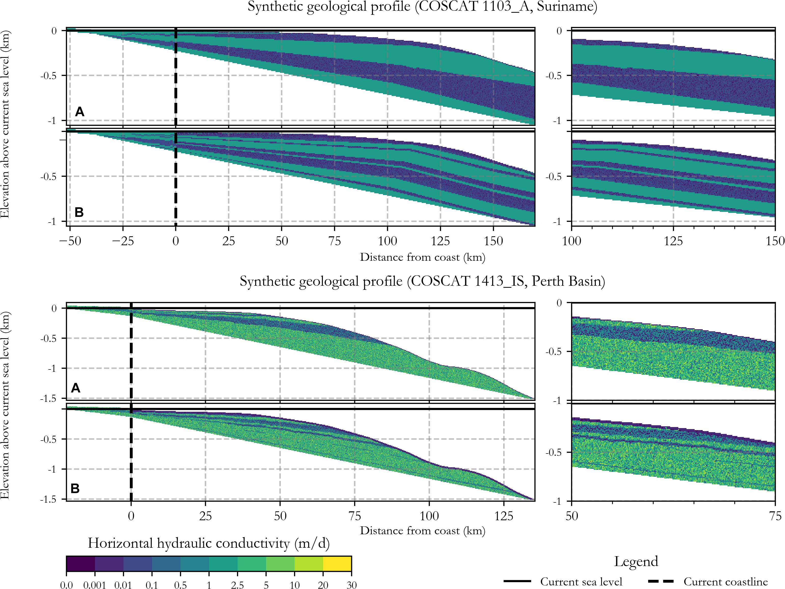
Figure 8. Examples of synthetic heterogenic coastal unconsolidated groundwater systems (CUGS) created using the geological heterogeneity algorithm described in section “Creating Synthetic Heterogenic Parameterization of Coastal Unconsolidated Groundwater Systems (CUGSs).” Randomly generated system with (A) two low and high stand layer combinations and (B) five such layers is presented for each of the two COSCAT regions considered in this example.

The hydraulic conductivity values are based on the GLHYMPS (Gleeson et al., 2014) and GUM (Huscroft et al., 2018) values randomly selected for each model cell based on their lognormal distribution in each selected COSCAT region. Therefore, in certain COSCAT regions, the hydraulic conductivity pattern can appear grainy if the standard deviation of the lognormal distribution is high (e.g., like COSCAT 1413_IS).

Comparison of Two Modeling Concepts to Estimate OFGVs Under Geological Uncertainty

In this section, we analyze the effects of the two modeling concepts on the simulated averaged groundwater salinity profiles and resulting FGFs and OFGVs. This analysis is performed over various stretches of the SEAWAT model domain (inland, continental shelf, and whole offshore domains) and by investigating the change in groundwater salinity over time (e.g., through an analysis of the system inertia).

Fresh Groundwater Fractions (FGFs) in Coastal Zones

The inland domain is entirely composed of fresh groundwater (drinking water, < 0.5 g TDS/L) in most models within the selected set of seven COSCAT regions, coastal (ARP) types, and modeling concepts. The difference between the outcomes of the two modeling concepts in the inland domain is thus negligible. However, larger differences in mean estimated FGFs between the modeling concepts can be found in the continental shelf domains. The difference exceeds 10% in only one-third of the cases while maximum difference is 20.5% (COSCAT 403, North Sea region). A similar trend is observed for estimates regarding the FGFs in the whole offshore domain (only one region has difference larger than 10%). Even in cases with larger differences in mean estimated values, the standard deviations are relatively large and mostly overlap each other suggesting a reasonably good fit (e.g., COSCAT region 403_A in Figure 9, exact values in Supplementary Material). The estimated FGFs for the selected COSCAT regions and their respective ARPs are given in the Supplementary Material.

FIGURE 9

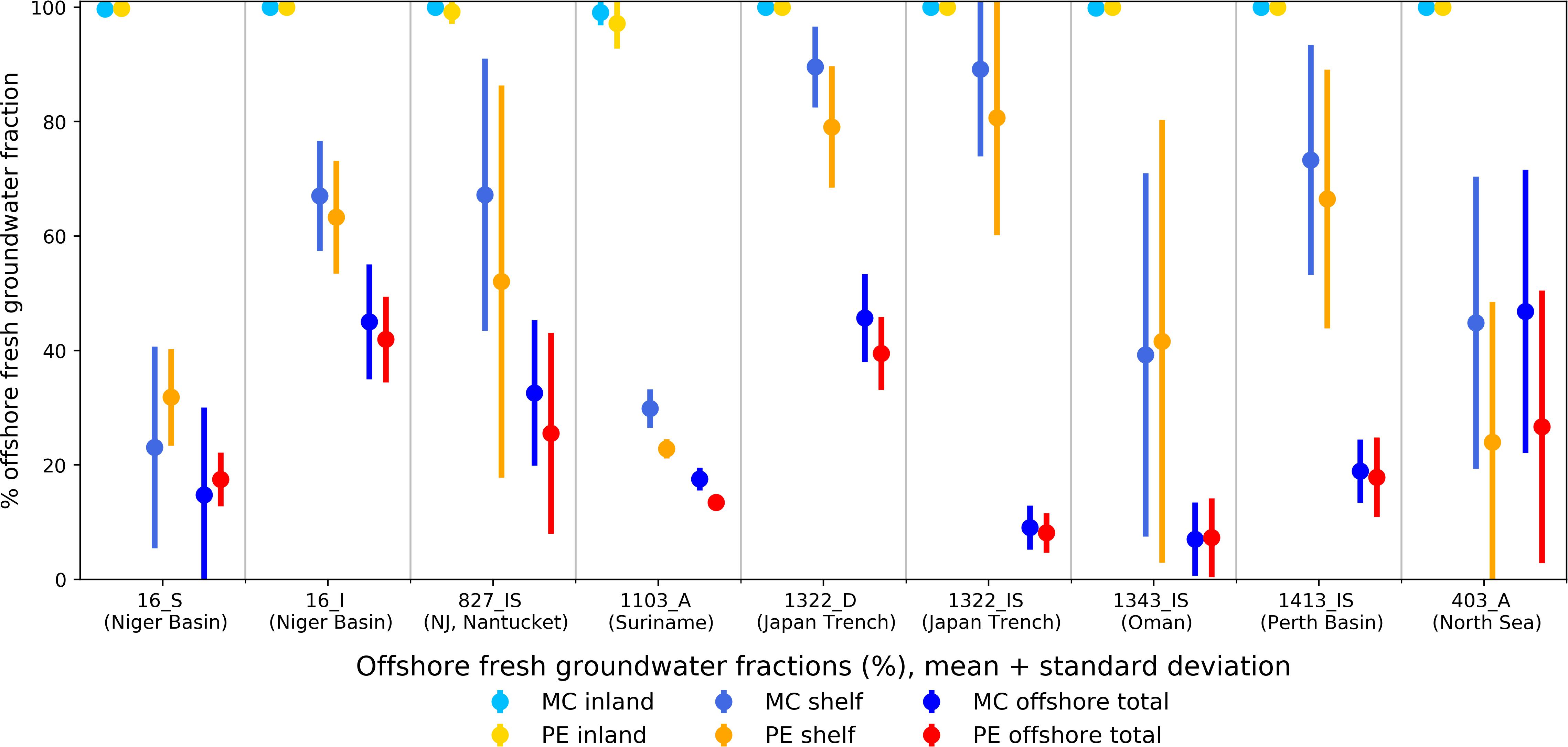
Figure 9. Estimated mean and standard deviation present-day offshore FGFs for both modeling concepts and the seven selected COSCAT regions and their respective coastal types considered.

Overall, the averaged estimated FGFs for continental shelf domains suggest that in most regions, there is a high probability of substantial fresh offshore reserves ranging from the lowest value of 22.8% (COSCAT 1103, Suriname) to the highest of almost 90% (COSCAT 1322, Japan Trench). The low FGF estimated for COSCAT 1103 region can be explained by a lengthy continental shelf domain that is largely filled with saline water (see Figure 10). The estimated average groundwater salinity distributions show no large differences between the two modeling concepts outcomes except wider brackish zones suggested by the MC model outcome. This is probably due to a larger number of model realizations using MC leading to higher variability across individual groundwater salinity profiles.

FIGURE 10

Figure 10. Averaged groundwater salinity profiles for both modeling concepts at four timeframes for COSCAT 1103_A region (Suriname). The estimated groundwater salinity in the 2D profiles is represented: (A) at the end of SP 0, groundwater salinity before fluctuating sea-level SPs; (B) at the lowest sea level occurring at the end of the sea-level drop represented by SP 21; (C) after the relatively fast sea-level rise back to the current sea level at the end of SP 31; and finally (D) estimation of future conditions in 20 ka from present at the end of SP 31_DSP. The results of the other eight SEAWAT models are provided in the Supplementary Material.

Regional Hydrogeological System Inertia

Assessing the rate of change in the estimated groundwater salinity profiles provides an important insight into the behavior of regional CUGSs and OFGVs stored therein over time. In such a way, we can better evaluate the non-renewability of the OFGVs. Figure 11 shows the evolution of mean (and standard deviation) FGF in the future 20 ka assuming constant sea level equal to the current situation (also other stresses remain the same). The predicted FGF trends of both modeling concepts are almost identical for all seven selected COSCAT regions showing a varying degree of gradual decline. The estimated mean FGF in the continental shelf domain eventually drops below 25% in all but one COSCAT regions (1322_IS), reaching almost zero values in five out of nine cases.

FIGURE 11

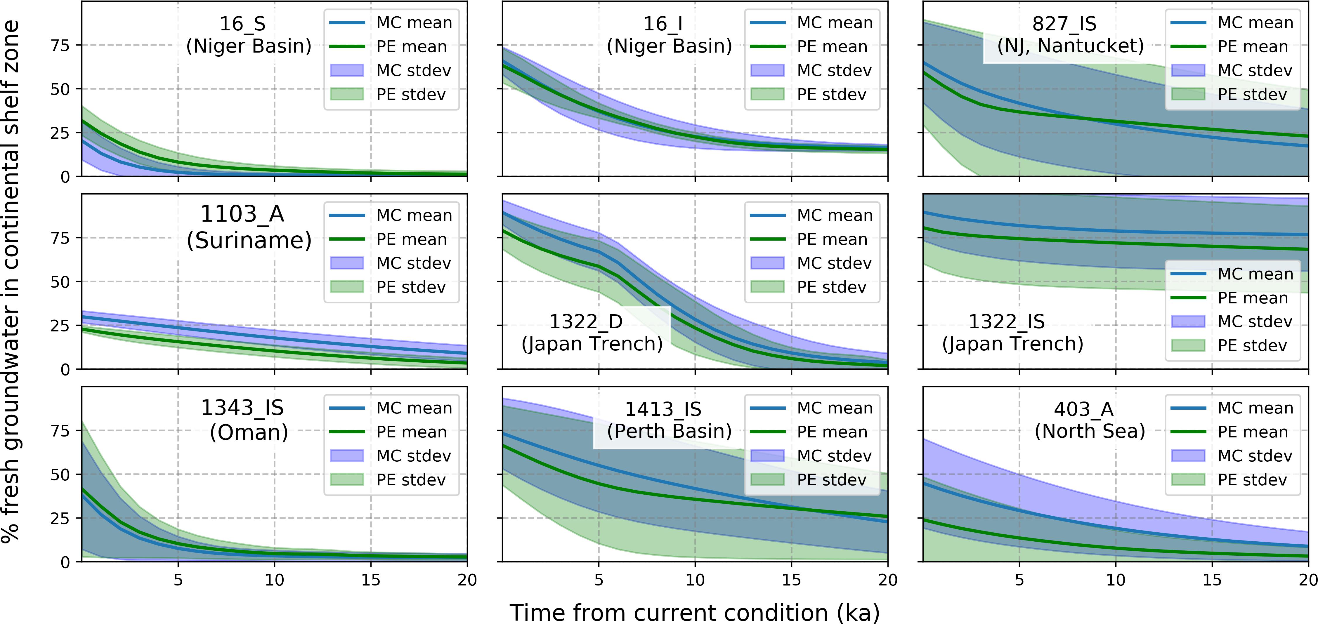
Figure 11. Estimated FGFs in the continental shelf domain for selected COSCAT regions (and respective coastal types) and both modeling concepts during the SP31_DSP time period. The current condition represents the estimated fractions at present time (here year = 0).

Model Runtime Difference Between PE and MC

The average SEAWAT model runtime per one SEAWAT model simulation for all selected COSCAT regions is almost identical for both PE and MC model concepts (46 and 40 h, respectively). COSCAT region 827_IS has the highest average model runtimes for the two modeling concepts with 133 h (PE) and 86 h (MC). Two COSCAT regions show the lowest average model runtimes (both 16 h) for the MC modeling concept (403_A and 1413_IS) and very close average runtime values for the PE modeling concept (12 and 10 h, respectively). Logically, the larger number of simulations in the MC modeling concept (100) to PE (24) leads to proportionally larger total model runtimes for all seven selected COSCAT regions. The total simulation time for all PE and MC models is 10,031 and 35,763 h, respectively. Final SEAWAT model runtimes (average and total) for all the selected COSCAT regions and ARPs are shown in the Supplementary Material.

Influence of Geological Settings on Offshore Fresh Groundwater Fraction Estimation

Out of the four geological parameters varied across the SEAWAT model simulations and both modeling concepts the thickness of the offshore clay cap layer has the most influence on estimate FGFs. SEAWAT model simulations with thicker offshore clay capping layers show above average (positive values on Y-axis) estimated FGF values (see Figure 12). The second most influential parameter is the number of aquifer and aquitard layers present in the synthetic heterogenic CUGS. SEAWAT model simulations with lower count of these layer combinations display on average somewhat above average estimated FGFs. However, the trend is not explicitly apparent (see Figure 12), since some of the simulations with lower number of aquifer and aquitard layers also show lower than average estimated FGFs. Variations of the other two geological parameters do not show any discernible influence on the estimated FGFs.

FIGURE 12

Figure 12. Influence of geological parameters on estimated FGFs (compared to mean value for each selected COSCAT region). Positive values correspond to SEAWAT models that estimate larger FGFs than average.

The Estimation of Offshore Fresh Groundwater Volumes (OFGVs)

High estimated FGF values do not necessarily mean large OFGV as these depend largely on the physical dimensions of the COSCAT region and its corresponding ARP. Table 3 provides the values of the calculated fresh (and brackish) offshore groundwater volume for the selected COSCAT regions and shows that some areas can contain several tens of thousands cubic kilometers of fresh groundwater in the continental shelf domain (i.e., East coast United States: New Jersey and Nantucket subregions). The fraction and corresponding volume of brackish water were calculated in the same manner as FGF and OFGV values but with different span of salinity concentration (0.5–10 g TDS/L).

TABLE 3

Table 3. Estimated offshore fresh (and brackish in brackets behind the OFGV value) groundwater volumes for the seven selected sample COSCAT regions (and respective coastal types); p = effective porosity (−).

Discussion

In our study, we adapt and combine a geological heterogeneity algorithm with a collection of global datasets showing that it is possible to successfully estimate first-order quantifications of the global geological heterogeneity of regional CUGSs. This involves derivation of various geological parameters and their subsequent application in generating synthetic profiles (ARPs) allowing heterogenic CUGS simulations. The ARPs then serve as hydrogeological schematizations in SEAWAT models which compute variable-density groundwater flow with coupled salt transport. Further implications and hypotheses are discussed in more detail in the sections below.

Estimating Global CUGS Geological Heterogeneity

The three derived and quantified geological parameters (aquitard patchiness, sand/mud composition ratio, sediment supply; see Figure 7) provide a satisfactory geological classification of CUGS worldwide. This parameterization is a first step to quantify geological heterogeneity of CUGS and can be directly used as input to large-scale hydrogeological (e.g., SEAWAT) models. However, despite the auspicious outcome of our study, feeding relatively simple conceptual models dealing with continental shelf architecture by available global datasets requires simplifications and assumptions since some information is still not available on such a large scale.

Major simplifications are made in establishing the relative sea-level change rate which can have an impact on estimated accommodation factor (see Eq. 1) by assuming a constant average absolute sea level globally (Pirazzoli, 1997). By implementing a sea-level fluctuation over multiple glacial–interglacial cycles and taking into account regional variations in sea levels, it would be possible to indicate shelves where either amplified (far from ice sheets) or subdued (near to ice sheets) sea-level low stands occur leading to, i.e., arguably more accurate dispersion modifier estimation. Furthermore, improving the accuracy of the thermal subsidence and compaction values could improve the geological estimation outcome in shelves positioned on lithosphere older than 70 Ma and in relatively thin sediment successions (compaction). Expanding the spatial and temporal knowledge on sediment accumulation on continental shelves beyond the areas investigated by Walsh and Nittrouer (2009) would lead to an improved accuracy of the dispersion modifier assessment. This would help to account for situations where not all sediments discharged from the continents accumulate on the shelf. Additional improvements can be achieved by accounting for changes in climate and drainage area size over the time period instead of assuming constant conditions as in the current state of the geological model.

SEAWAT Modeling of OFGVs

Combining the estimated geological heterogeneity parameterization results with the developed modeling concepts describing the geological structure of coastal areas formed by unconsolidated sediments. This allows us to build synthetic hydrogeological CUGSs represented as interlaid aquifer–aquitard layer combinations. Nevertheless, there are still several parameters that are to be estimated to improve the accuracy of simulating regional scale CUGS in the coastal zones. This would have required a large data collection effort of geological boreholes and hydrogeological profiles that is beyond the scope of this study. Performing this data collection could extend the use of the hereby presented approach to build more detailed local scale hydrogeological models, as in the current state, the ARP methodology is fit only for regional scale applications.

Our SEAWAT modeling approach consisted of setting up two modeling concepts to deal with geological uncertainty to investigate the temporal variation in groundwater salinity profiles and potential presence of OFGVs in seven selected COSCAT regions. The idea to achieve comparable estimation results with lower numerical proved successful. This result gains further significance when we take into account that we only selected seven COSCAT regions (= nine ARPs) out of 127 for our geological heterogeneity parameterization study. Approximately 508,000 computation hours would be necessary if one would extent the MC modeling concept to the rest of the COSCAT regions (see Geological Heterogenic Parameterization COSCAT regions in Figure 5). This is a significant difference compared to 140,208 computation hours with the PE modeling concept that results in similar simulated OFGVs.

Our SEAWAT model simulations for the seven selected COSCAT region (apart from Figure 10, see Supplementary Material for eight other salinity profiles) show that there are potentially large OFGVs stored in continental shelves worldwide as suggested by Post et al. (2013). Accounting for different coastal types shows that the presence and magnitude of these OFGVs can vary within a single COSCAT region. The non-renewability and potential short-term presence (from a geological point of view) of these OFGVs is demonstrated by extending the SEAWAT models beyond the present timeline (by 20 ka) (see section “Regional Hydrogeological System Inertia”). In our approach, we assessed the diminishing trend of OFGV by maintaining the current sea level (0 m asl) over a period of 20 ka showing a rapid decline (from a geological point of view) in FGFs in the continental shelf domain in most selected COSCAT regions (Figure 11).

Considering a time scale stretching over more than one full glacial–interglacial cycle (> 125 ka) allows us to simulate the effect of sea-level change on the estimated groundwater salinity profile. Leaving out overwash events has negligible impact on the simulated OFGVs because the temporal impacts of these events on the groundwater salinity are likely limited to decades (Yu et al., 2016) which is beyond the temporal resolution of our SEAWAT modeling approach. However, these events can have a relatively large influence on the inland domain of the local groundwater salinity profiles (Michael et al., 2016; Yang et al., 2018) and should be considered when building local models with higher temporal resolution. The influence of rivers on groundwater recharge in the inland part of the model domain was also omitted in our study. This potentially leads to higher groundwater fluxes in the seaward direction and over-estimation of OFGVs. However, we believe that this issue is compensated by limiting the recharge rates to hydraulic conductivity values of the upper most model cells. Furthermore, implementing rivers into cross-sectional 2D groundwater flow models is highly uncertain and untested and realizing that is well beyond the scope of this study. Additionally, given the large climate changes that occurred during the last glacial–interglacial period (e.g., Fleitmann et al., 2003), including a more detailed paleo precipitation (and thus groundwater recharge) estimations could increase the accuracy (and reliability) of our OFGVs estimations.

While analyzing the influence of geological settings on OFGVs, we found that only one (out of four) geological parameter has discernible effects on the simulated groundwater salinity distribution. The presence and thickness of offshore clay cap layer in the continental shelf and/or continental slope domains shows the largest influence on the groundwater salinity distribution. Groundwater systems with thicker offshore clay cap layers show larger FGFs in the continental shelf domain, suggesting fresh groundwater deposition during sea-level low stand period and subsequent shielding this off from mixing with infiltrated sea water through the offshore clay cap layer deposited shortly afterward. This implies that large non-renewable OFGVs can be trapped under such (very) low permeable clay capping layers deposited on the ocean floor during a sea-level low stand period. The number of preserved aquifer–aquitard layer combinations, deposited during low and high stands, respectively, also influences the simulated groundwater salinity in the 2D profiles. Arguably, groundwater systems with a higher number of such sequences tend to have thinner or discontinuous aquitards that allow for easier vertical salt water intrusion with rising sea levels as shown by Kooi et al. (2000), Kooi and Groen (2001, 2003), Post et al. (2013).

The OFGVs expressed as per stretch kilometer of coastline are compared with values reported by Post et al. (2013) in two sample COSCAT regions. In the Suriname continental shelf domain, our OFGV estimate amounts to 5.1 km³/km (compared to 6.3 km³/km reported by Post et al., 2013) and 7.5 km³/km (compared to 4.8 km³/km reported by Post et al., 2013) in the New Jersey and Nantucket continental shelf domain. The total volumes of potentially usable groundwater (e.g., also for desalination purposes) further increase if we take into account the potential use of brackish water (see Table 3). In the case of New Jersey and Nantucket continental shelf domain, our modeled OFGV is overestimated by roughly 30% compared to the reported value by Post et al. (2013). This could be due to constant porosity value applied in our SEAWAT models (0.3), which in this case is one-third higher than the porosity reported by Post et al. (2013) amounting to 0.2. However, changing porosity values could also lead to a different estimated salinity distribution and assuming a linear change in OFGV while varying the porosity parameter is an oversimplification. This discrepancy further stresses the importance of additional geological inputs to improve the performance of the methodology presented in this study. This discrepancy further stresses the importance of additional geological inputs to improve the performance of the methodology presented in this study. Even though in our study we purely focus on OFGVs occurrence, similar conceptual models could be applied to investigate the effects of other stress factors on fresh groundwater resources in coastal zones (e.g., increased human extraction rates, climate change effects including future sea-level rise and groundwater recharges, and possible mitigation strategies like aquifer storage and recovery). This can help regional water management bodies to investigate the possibility of tapping the OFGV to be then used as a potential supplementary supply of fresh water or as feedwater to desalination plants.

Summary and Conclusion

The need for a better understanding and definition of heterogeneous coastal hydrogeology at the global scale is addressed in this study by combining various conceptual geological models with state-of-the-art freely available global datasets. The combination of these is used as input into the global geological heterogeneity algorithm. Even though only three geological parameters are explicitly quantified (another four need to be randomized), we show that adequate information is provided to create synthetic heterogenic CUGSs.

These synthetic heterogenic CUGSs are used as input to SEAWAT models (using the SEAWAT code), simulating variable-density groundwater flow and coupled salt transport. The SEAWAT models estimate FGFs and OFGVs over the past glacial–interglacial cycle and extending to the near future. Thus, we are able to estimate the magnitude and future decrease of OFGVs in seven selected COSCAT regions. Comparing the estimated OFGVs with literature values for the selected COSCAT regions shows a potential for expanding the hereby presented methodology to the rest of coastal COSCAT regions worldwide (being 127 in number). By extending our approach to the global coastline, thus we would gain valuable insights into current and near future OFGV occurrence and magnitude in CUGSs. The analysis of the influence of geological settings on OFGVs shows that the presence and thickness of an offshore low permeable (e.g., clay) layer overtopping the more permeable offshore aquifers has the highest positive influence on simulated OFGV. Therefore, the focus of the geological data collection should not be limited to the inland areas but should also include as many offshore locations as possible.

Four geological parameters could not be quantified within the scope of this study. To overcome this, two different modeling concepts were designed to randomize the values of these geological parameters for seven selected COSCAT regions (= nine ARPs). The first modeling concept only takes into account the extreme values of the geological heterogeneity parameter values (PE) resulting in 24 SEAWAT models in total. The second modeling concept is based on a randomized MC randomization of the geological heterogeneity parameter values and amounts to 100 SEAWAT models. The average groundwater salinity profiles calculated by these two modeling concepts showed to yield very similar results. This means that using the PE-method to estimate averaged regional OFGVs results in a 75% reduction in total SEAWAT model runtimes, while maintaining the same degree of confidence in the model outcome as when conducting a full MC simulation. This is an important implication for future global and large regional modeling studies dealing with missing geological information on such large scales. Collecting local coastal geological data (e.g., borehole datasets) and implementing these into the conceptual geological model would be a logical next step in clearing the path to a better understanding and quantification of global hydrogeological heterogeneity, leading to improved water management strategies and decision making. The hereby presented new dataset and methods can be applied on a regional scale (tens to hundreds of kilometers) to investigate the effects of geological heterogeneity in coastal unconsolidated systems on OFGVs presence and to quantify their magnitude.

Data Availability Statement

The datasets generated for this study are available on request to the corresponding author.

Author Contributions

Primary author DZ wrote the initial version of manuscript and conducted the whole SEAWAT modeling study and implementation of the geological heterogeneity. The latter was the topic of MK’s M.Sc. thesis under supervision of DZ and KC. MB and GO provided guidance throughout the whole study and the direction of the research. Furthermore, they helped improved the quality of the final manuscript version.

Funding

This research was partially funded by the Netherlands Organization for Scientific Research (NWO) and the Ministry of Infrastructure and Water Management under TTW Perspectives Program Water Nexus (Project No. 14298).

Conflict of Interest

The authors declare that the research was conducted in the absence of any commercial or financial relationships that could be construed as a potential conflict of interest.

Acknowledgments

We thank reviewers for their thorough reading and comments that have considerably improved the quality of this manuscript. The modeling study was carried out on the Dutch national e-infrastructure (HPC Cartesius) with the support of SURF Cooperative.

Supplementary Material

The Supplementary Material for this article can be found online at: https://www.frontiersin.org/articles/10.3389/feart.2019.00339/full#supplementary-material

References

Bridge, J. S. (2009). Rivers and Floodplains: Forms, Processes, and Sedimentary Record. Hoboken, NY: Wiley-Blackwell.

Google Scholar

Cardenas, M. B., Bennett, P. C., Zamora, P. B., Befus, K. M., Rodolfo, R. S., Cabria, H. B., et al. (2015). Devastation of aquifers from tsunami-like storm surge by Supertyphoon Haiyan. Geophys. Res. Lett. 42, 2844–2851. doi: 10.1002/2015GL063418

CrossRef Full Text | Google Scholar

Carretero, S., Rapaglia, J., Bokuniewicz, H., and Kruse, E. (2013). Impact of sea-level rise on saltwater intrusion length into the coastal. Cont. Shelf Res. 61–62, 62–70. doi: 10.1016/j.csr.2013.04.029

CrossRef Full Text | Google Scholar

Cattaneo, A., and Steel, R. J. (2003). Transgressive deposits: a review of their variability. Earth Sci. Rev. 62, 187–228. doi: 10.1016/S0012-8252(02)00134-4

CrossRef Full Text | Google Scholar

Chui, T. F. M., and Terry, J. P. (2015). Groundwater salinisation on atoll islands after storm-surge flooding: modelling the influence of central topographic depressions. Water Environ. J. 29, 430–438. doi: 10.1111/wej.12116

CrossRef Full Text | Google Scholar

Cobaner, M., Yurtal, R., Dogan, A., and Motz, L. H. (2012). Three dimensional simulation of seawater intrusion in coastal aquifers: a case study in the Goksu Deltaic Plain. J. Hydrol. 464–465, 262–280. doi: 10.1016/j.jhydrol.2012.07.022

CrossRef Full Text | Google Scholar

Cohen, D., Person, M., Wang, P., Gable, C. W., Hutchinson, D., Marksamer, A., et al. (2010). Origin and extent of fresh paleowaters on the atlantic continental shelf, USA. Ground Water 8, 143–158. doi: 10.1111/j.1745-6584.2009.00627.x

PubMed Abstract | CrossRef Full Text | Google Scholar

Cohen, K. M., and Lobo, F. J. P. (2013). Continental shelf drowned landscapes: submerged geomorphological and sedimentary record of the youngest cycles. Geomorphology 203, 1–5. doi: 10.1016/j.geomorph.2013.09.006

CrossRef Full Text | Google Scholar

Custodio, E. (2002). Aquifer overexploitation: what does it mean? Hydrogeol. J. 10, 254–277. doi: 10.1007/s10040-002-0188-6

CrossRef Full Text | Google Scholar

Dutkiewicz, A., Müller, R. D., O’Callaghan, S., and Jónasson, H. (2015). Census of seafloor sediments in the world’s ocean. Geology 43, 795–798. doi: 10.1130/G36883.1

CrossRef Full Text | Google Scholar

Edmunds, W. M., and Milne, C. J. (2001). Palaeowaters in Coastal Europe:Evolution of Groundwater Sincethe Late Pleistocene. Special Publication 189. Bath: Geological Society Publishing House.

Google Scholar

Ehlers, J., and Gibbard, P. L. (2004). Quaternary Glaciations Extent and Chronology, Volume 2. ed. Developments in Quaternary Sciences. Amsterdam: Elsevier.

Google Scholar

Ferguson, G., and Gleeson, T. (2012). Vulnerability of coastal aquifers to groundwater use and climate change. Nat. Clim. Chang 2, 342–345. doi: 10.1038/nclimate1413

CrossRef Full Text | Google Scholar

Fan, Y., Miguez-Macho, G., Jobbágy, E. G., Jackson, R. B., and Otero-Casal, C. (2017). Hydrologic regulation of plant rooting depth. Proc. Natl. Acad. Sci. 114: 201712381. doi: 10.1073/pnas.1712381114

PubMed Abstract | CrossRef Full Text | Google Scholar

Fleitmann, D., Burns, S. J., Mudelsee, M., Neff, U., Kramers, J., Mangini, A., et al. (2003). Holocene forcing of the indian monsoon recorded in a stalagmite from southern oman. Science 300, 1737–1739. doi: 10.1126/science.1083130

PubMed Abstract | CrossRef Full Text | Google Scholar

Ghaffour, N., Missimer, T. M., and Amy, G. L. (2013). Technical review and evaluation of the economics of water desalination: current and future challenges for better water supply sustainability. Desalination 309, 197–207. doi: 10.1016/j.desal.2012.10.015

CrossRef Full Text | Google Scholar

Gingerich, S. B., Voss, C. I., and Johnson, A. G. (2017). Seawater-flooding events and impact on freshwater lenses of low-lying islands: controlling factors, basic management and mitigation. J. Hydrol. 551, 676–688. doi: 10.1016/j.jhydrol.2017.03.001

CrossRef Full Text | Google Scholar

Gleeson, T., Befus, K. M., Jasechko, S., Luijendijk, E., and Cardenas, M. B. (2015). The global volume and distribution of modern groundwater. Nat. Geosci. 9, 161–167. doi: 10.1038/NGEO2590

PubMed Abstract | CrossRef Full Text | Google Scholar

Gleeson, T., Luijendijk, E., Mcdonnell, J. J., Taylor, R. G., and Wada, Y. (2017). Global aquifers dominated by fossil groundwaters but wells vulnerable to modern contamination. Nat. Geosci. 10, 425–430. doi: 10.1038/NGEO2943

CrossRef Full Text | Google Scholar

Gleeson, T., Moosdorf, N., Hartmann, J., and Van Beek, L. P. H. (2014). A glimpse beneath earth’s surface: GLobal HYdrogeology MaPS (GLHYMPS) of permeability and porosity. Geophys. Res. Lett. 41, 3891–3898. doi: 10.1002/2014GL059856

CrossRef Full Text | Google Scholar

Grant, K. M., Rohling, E. J., Bar-Matthews, M., Ayalon, A., Medina-Elizalde, M., Ramsey, C. B., et al. (2012). Rapid coupling between ice volume and polar temperature over the past 150,000?years. Nature 491, 744–747. doi: 10.1038/nature11593

PubMed Abstract | CrossRef Full Text | Google Scholar

Groen, J., Velstra, J., and Meesters, A. G. C. A. (2000). Salinization processes in paleowaters in coastal sediments of Suriname: evidence from d 37 Cl analysis and diffusion modelling. J. Hydrol. 234, 1–20. doi: 10.1016/s0022-1694(00)00235-3

CrossRef Full Text | Google Scholar

Gustafson, C., Key, K., and Evans, R. L. (2019). Aquifer systems extending far offshore on the U.S. Atlantic margin. Sci. Rep. 9, 1–10. doi: 10.1038/s41598-019-44611-7

PubMed Abstract | CrossRef Full Text | Google Scholar

Hanebuth, T. J., Stattegger, K., and Saito, Y. (2002). The stratigraphic architecture of the central Sunda Shelf (SE Asia) recorded by shallow-seismic surveying. Geo Mar. Lett. 22, 86–94. doi: 10.1007/s00367-002-0102-1

CrossRef Full Text | Google Scholar

Hartmann, J., and Moosdorf, N. (2012). The new global lithological map database GLiM: a representation of rock properties at the Earth surface. Geochem. Geophys. Geosyst. 13, 1–37. doi: 10.1029/2012GC004370

CrossRef Full Text | Google Scholar

Hayes, M. O. (1966). “Relationship between coastal climate and bottom sediment type on the inner continental shelf,” in Marine Geology (Amsterdam: Elsevier Publishing Company).

Google Scholar

Head, M. J., and Gibbard, P. L. (2005). Early-Middle Pleistocene Transitions: The Land-ocean Evidence. London: Geological Society of London, doi: 10.1144/GSL.SP.2005.247

CrossRef Full Text | Google Scholar

Hengl, T., De Jesus, J. M., MacMillan, R. A., Batjes, N. H., Heuvelink, G. B. M., Ribeiro, E., et al. (2014). SoilGrids1km - Global soil information based on automated mapping. PLoS One 9:e105992. doi: 10.1371/journal.pone.0105992

PubMed Abstract | CrossRef Full Text | Google Scholar

Huang, P., and Chiu, Y. (2018). A simulation-optimization model for seawater intrusion management at pingtung coastal. Water 10:251. doi: 10.3390/w10030251

CrossRef Full Text | Google Scholar

Huscroft, J., Gleeson, T., Hartmann, J., and Börker, J. (2018). Compiling and mapping global permeability of the unconsolidated and consolidated earth: global hydrogeology MaPS 2.0 (GLHYMPS 2.0). Geophys. Res. Lett. 45, 1897–1904. doi: 10.1002/2017GL075860

CrossRef Full Text | Google Scholar

Jones, E., Qadir, M., Van Vliet, M. T. H., Smakhtin, V., and Kang, S. (2019). The state of desalination and brine production: a global outlook. Sci. Total Environ. 657, 1343–1356. doi: 10.1016/j.scitotenv.2018.12.076

PubMed Abstract | CrossRef Full Text | Google Scholar

Karner, G. D., and Watts, A. B. (1982). On isostasy at Atlantic-type continental margins. J. Geophys. Res. 87, 2923–2948. doi: 10.1029/JB087iB04p02923

CrossRef Full Text | Google Scholar

Ketabchi, H., Mahmoodzadeh, D., Ataie-Ashtiani, B., and Simmons, C. T. (2016). Sea-level rise impacts on seawater intrusion in coastal aquifers: review and integration. J. Hydrol. 535, 235–255. doi: 10.1016/j.jhydrol.2016.01.083

CrossRef Full Text | Google Scholar

Ketabchi, H., Mahmoodzadeh, D., Ataie-Ashtiani, B., Werner, A. D., and Simmons, C. T. (2014). Sea-level rise impact on fresh groundwater lenses in two-layer small islands. Hydrol. Process. 28, 5938–5953. doi: 10.1002/hyp.10059

CrossRef Full Text | Google Scholar

Knight, A. C., Werner, A. D., and Morgan, L. K. (2018). The onshore influence of offshore fresh groundwater. J. Hydrol. 561, 724–736. doi: 10.1016/j.jhydrol.2018.03.028

CrossRef Full Text | Google Scholar

Kooi, H., and Groen, J. (2001). Offshore continuation of coastal groundwater systems; predictions using sharp-interface approximations and variable-density flow modelling. J. Hydrol. 246, 19–35. doi: 10.1016/S0022-1694(01)00354-7

CrossRef Full Text | Google Scholar

Kooi, H., and Groen, J. (2003). Geological processes and the management of groundwater resources in coastal areas. Netherlands J. Geosci. 82, 31–40. doi: 10.1017/s0016774600022770

CrossRef Full Text | Google Scholar

Kooi, H., Groen, J., and Leijnse, A. (2000). Modes of seawater intrusion during transgressions. Water Resour. Res. 36, 3581–3589. doi: 10.1029/2000WR900243

CrossRef Full Text | Google Scholar

Lambeck, K., Rouby, H., Purcell, A., Sun, Y., and Sambridge, M. (2014). Sea level and global ice volumes from the Last Glacial Maximum to the Holocene. Proc. Natl. Acad. Sci. U.S.A. 111, 15296–15303. doi: 10.1073/pnas.1411762111

PubMed Abstract | CrossRef Full Text | Google Scholar

Langevin, C. D., Thorne, D. T. J., Dausman, A. M., Sukop, M. C., and Guo, W. (2008). SEAWAT version 4: a computer program for simulation of multi-species solute and heat transport. U.S. Geol. Surv. Tech. Methods B. 6:39.

Google Scholar

Laruelle, G. G., Dürr, H. H., Lauerwald, R., Hartmann, J., Slomp, C. P., Goossens, N., et al. (2013). Global multi-scale segmentation of continental and coastal waters from the watersheds to the continental margins. Hydrol. Earth Syst. Sci. 17, 2029–2051. doi: 10.5194/hess-17-2029-2013

CrossRef Full Text | Google Scholar

Mabrouk, M., Jonoski, A., Oude Essink, G. H. P., and Uhlenbrook, S. (2018). Impacts of sea level rise and groundwater extraction scenarios on fresh groundwater resources. Water 10, 1–14. doi: 10.3390/w10111690

CrossRef Full Text | Google Scholar

Mahmoodzadeh, D., and Karamouz, M. (2019). Seawater intrusion in heterogeneous coastal aquifers under flooding events. J. Hydrol. 568, 1118–1130. doi: 10.1016/j.jhydrol.2018.11.012

CrossRef Full Text | Google Scholar

Masson-Delmotte, V., Zhai, P., Pörtner, H. O., Roberts, D., Skea, J., and Shukla, P. R., et al. eds (2018). “IPCC, 2018: Summary for Policymakers,” in Global Warming of 1.5°C. An IPCC Special Report on the Impacts of Global Warming of 1.5°C Above Pre-Industrial Levels and Related Global Greenhouse Gas Emission Pathways, in the Context of Strengthening the Global, (Geneva: IPCC).

Google Scholar

Meisler, H., Leahy, P. P., and Knobel, L. L. (1984). Effect of Eustatic Sea-Level Changes on Saltwater-Freshwater in the Northern Atlantic Coastal Plain. Washington, DC: United States Government Publishing Office.

Google Scholar

Meybeck, M., Dürr, H. H., and Vörösmarty, C. J. (2006). Global coastal segmentation and its river catchment contributors: a new look at land-ocean linkage. Glob. Biogeochem. Cycles 20, 1–15. doi: 10.1029/2005GB002540

CrossRef Full Text | Google Scholar

Miall, A. D. (2014). Fluvial Depositional Systems. Berlin: Springer, doi: 10.1007/978-3-319-00666-6

CrossRef Full Text | Google Scholar

Micallef, A., Mountjoy, J. J., Schwalenberg, K., Jegen, M., Bradley, W. A., Woelz, S., et al. (2018). How offshore groundwater shapes the seafloor. Eos 99, 1–8. doi: 10.1029/2018EO090691

CrossRef Full Text | Google Scholar

Michael, H. A., Post, V. E. A., Wilson, A. M., and Werner, A. D. (2017). Science, society, and the coastal groundwater squeeze. Water Resour. Res. 53, 2610–2617. doi: 10.1002/2017WR020851

CrossRef Full Text | Google Scholar

Michael, H. A., Russoniello, C. J., and Byron, L. A. (2013). Global assessment of vulnerability to sea-level rise in topography-limited and recharge-limited coastal groundwater systems. Water Resour. Res. 49, 2228–2240. doi: 10.1002/wrcr.20213

CrossRef Full Text | Google Scholar

Michael, H. A., Scott, K. C., Koneshloo, M., Yu, X., Khan, M. R., and Li, K. (2016). Geologic influence on groundwater salinity drives large seawater circulation through the continental shelf. Geophys. Res. Lett. 43, 10782–10791. doi: 10.1002/2016GL070863

CrossRef Full Text | Google Scholar

Montzka, C., Herbst, M., Weihermüller, L., Verhoef, A., and Vereecken, H. (2017). A global data set of soil hydraulic properties and sub-grid variability of soil water retention and hydraulic conductivity curves. Earth Syst. Sci. Data. 9, 529–543. doi: 10.5194/essd-2017-13

CrossRef Full Text | Google Scholar

Morgan, L. K., Werner, A. D., and Patterson, A. E. (2018). A conceptual study of offshore fresh groundwater behaviour in the Perth Basin (Australia): modern salinity trends in a prehistoric context. J. Hydrol. Reg. Stud. 19, 318–334. doi: 10.1016/j.ejrh.2018.10.002

CrossRef Full Text | Google Scholar

Müller, R. D., Sdrolias, M., Gaina, C., and Roest, W. R. (2008). Age, spreading rates, and spreading asymmetry of the world’s ocean crust. Geochem. Geophys. Geosyst. 9. doi: 10.1029/2007GC001743

CrossRef Full Text | Google Scholar

Nam, S. II, Stein, R., Grobe, H., and Hubberten, H. (1995). Late Quaternary glacial-interglacial changes in sediment composition at the East Greenland continental margin and their paleoceanographic implications. Mar. Geol. 122, 243–262. doi: 10.1016/0025-3227(94)00070-2

CrossRef Full Text | Google Scholar

NTSG, (2019). MODIS Global Evapotranspiration Project (MOD16) [WWW Document]. Available at: www.ntsg.umt.edu/project/modis/mod16.php (accessed August, 24 2019).

Google Scholar

Oude Essink, G. H. P., Van Baaren, E. S., and de Louw, P. G. B. (2010). Effects of climate change on coastal groundwater systems: a modeling study in the Netherlands. Water Resour. Res. 46, 1–16. doi: 10.1029/2009WR008719

CrossRef Full Text | Google Scholar

Pham, V. H., Van Geer, F. C., Bui Tran, V., Dubelaar, W., and Oude Essink, G. H. P. (2019). Paleo-hydrogeological reconstruction of the fresh-saline groundwater distribution in the vietnamese mekong delta since the late Pleistocene. J. Hydrol. Reg. Stud. 23:100594. doi: 10.1016/j.ejrh.2019.100594

CrossRef Full Text | Google Scholar

Pillans, B., Chappell, J., and Naish, T. R. (1998). A review of the Milankovitch climatic beat: template for Plio-Pleistocene sea-level changes and sequence stratigraphy. Sediment. Geol. 122, 5–21. doi: 10.1016/S0037-0738(98)00095-5

CrossRef Full Text | Google Scholar

Pinet, P. R. (2003). Invitation to Oceanography. Burlington, MA: Jones & Bartlett Learning.

Google Scholar

Pirazzoli, P. A. (1997). Sea-Level Changes: The Last 20,000 Years. Hoboken, NJ: Wiley.

Google Scholar

Pollard, D., and Deconto, R. M. (2016). Contribution of Antarctica to past and future sea-level rise. Nature 531, 591–597. doi: 10.1038/nature17145

PubMed Abstract | CrossRef Full Text | Google Scholar

Post, V. E. A., Groen, J., Kooi, H., Person, M., Ge, S., and Edmunds, W. M. (2013). Offshore fresh groundwater reserves as a global phenomenon. Nature 504, 71–78. doi: 10.1038/nature12858

PubMed Abstract | CrossRef Full Text | Google Scholar

Ranjan, P., Kazama, S., Sawamoto, M., and Sana, A. (2009). Global scale evaluation of coastal fresh groundwater resources. Ocean Coast. Manag. 52, 197–206. doi: 10.1016/j.ocecoaman.2008.09.006

CrossRef Full Text | Google Scholar

Rasmussen, P., Sonnenborg, T. O., Goncear, G., and Hinsby, K. (2013). Assessing impacts of climate change, sea level rise, and drainage canals on saltwater intrusion to coastal aquifer. Hydrol. Earth Syst. Sci. 17, 421–443. doi: 10.5194/hess-17-421-2013

CrossRef Full Text | Google Scholar

Reijenstein, H. M., Posamentier, H. W., and Bhattacharya, J. P. (2011). Seismic geomorphobgy and high-resolution seismic stratigraphy of inner-shelf fluvial, estuarine, deltaic, and marine sequences. Gulf of Thailand. Am. Assoc. Pet. Geol. Bull. 95, 1959–1990. doi: 10.1306/03151110134

CrossRef Full Text | Google Scholar

Reynolds, D. J., Steckler, M. S., and Coakley, B. J. (1991). The role of the sediment load in sequence stratigraphy: the influence of flexural isostasy and compaction. J. Geophys. Res. 96, 6931–6949. doi: 10.1029/90JB01914

CrossRef Full Text | Google Scholar

Sefelnasr, A., and Sherif, M. (2014). Impacts of seawater rise on seawater intrusion in the nile delta aquifer. Egypt Ground Water 52, 264–276. doi: 10.1111/gwat.12058

PubMed Abstract | CrossRef Full Text | Google Scholar

Smith, D. E., Harrison, S., Firth, C. R., and Jordan, J. T. (2011). The early holocene sea level rise. Quat. Sci. Rev. 30, 1846–1860. doi: 10.1016/j.quascirev.2011.04.019

CrossRef Full Text | Google Scholar

Solórzano-Rivas, S. C., and Werner, A. D. (2018). On the representation of subsea aquitards in models of offshore fresh groundwater. Adv. Water Resour. 112, 283–294. doi: 10.1016/j.advwatres.2017.11.025

CrossRef Full Text | Google Scholar

Stone, A., Lanzoni, M., and Smedley, P. (2019). “Groundwater Resources,” in Water Science, Policy, and Management: A Global Challenge, eds S. J. Dadson, D. E. Garrick, J. W. Penning-Rowsell, E. C. Hall, and R. H. Jocelyne Hughes, (Hoboken, NJ: Wiley), doi: 10.1002/9781119520627.ch3

CrossRef Full Text | Google Scholar

Syvitski, J. P. M., Peckham, S. D., Hilberman, R., and Mulder, T. (2003). Predicting the terrestrial flux of sediment to the global ocean: a planetary perspective. Sediment. Geol. 162, 5–24. doi: 10.1016/S0037-0738(03)00232-X

CrossRef Full Text | Google Scholar

Tessler, Z. D., Vörösmarty, C. J., Grossberg, M., Gladkova, I., Aizenman, H., Syvitski, J. P. M., et al. (2015). Profiling risk and sustainability in coastal deltas of the world. Science 349, 638–643. doi: 10.1126/science.aab3574

PubMed Abstract | CrossRef Full Text | Google Scholar

Thomas, A. T., Reiche, S., Riedel, M., and Clauser, C. (2019). The fate of submarine fresh groundwater reservoirs at the New Jersey shelf, USA. Hydrogeol. J. 27, 2673–2694. doi: 10.1007/s10040-019-01997-y

CrossRef Full Text | Google Scholar

United Nations, (2017). World Population Prospects: The 2017 Revision, Key Findings and Advance Tables (No. ESA/P/WP/248). New York, NY: United Nations.

Google Scholar

Van Engelen, J., Oude Essink, G. H. P., Kooi, H., and Bierkens, M. F. P. (2018). On the origins of hypersaline groundwater in the Nile Delta aquifer. J. Hydrol. 560, 301–317. doi: 10.1016/j.jhydrol.2018.03.029

CrossRef Full Text | Google Scholar

Waelbroeck, C., Labeyrie, L., Michel, E., Duplessy, J. C., McManus, J. F., Lambeck, K., et al. (2002). Sea-level and deep water temperature changes derived from benthic foraminifera isotopic records. Quat. Sci. Rev. 21, 295–305. doi: 10.1016/s0277-3791(01)00101-9

CrossRef Full Text | Google Scholar

Walsh, J. P., and Nittrouer, C. A. (2009). Understanding fine-grained river-sediment dispersal on continental margins. Mar. Geol. 263, 34–45. doi: 10.1016/j.margeo.2009.03.016

CrossRef Full Text | Google Scholar

Weatherall, P., Marks, K. M., Jakobsson, M., Schmitt, T., Tani, S., Arndt, J. E., et al. (2015). A new digital bathymetric model of the world’s oceans. Earth Space Sci. 2, 331–345. doi: 10.1002/2015EA000107

CrossRef Full Text | Google Scholar

Werner, A. D., Bakker, M., Post, V. E. A., Vandenbohede, A., Lu, C., Ataie-Ashtiani, B., et al. (2013). Seawater intrusion processes, investigation and management: recent advances and future challenges. Adv. Water Resour. 51, 3–26. doi: 10.1016/j.advwatres.2012.03.004

CrossRef Full Text | Google Scholar

Wu, Z., Li, J., Li, S., Shang, J., and Jin, X. (2017). A new method to identify the foot of continental slope based on an integrated profile analysis. Mar. Geophys. Res. 38, 199–207. doi: 10.1007/s11001-016-9273-4

CrossRef Full Text | Google Scholar

Yang, J., Graf, T., Herold, M., and Ptak, T. (2013). Modelling the effects of tides and storm surges on coastal aquifers using a coupled surface–subsurface approach. J. Contam. Hydrol. 149, 61–75. doi: 10.1016/j.jconhyd.2013.03.002

PubMed Abstract | CrossRef Full Text | Google Scholar

Yang, J., Zhang, H., Yu, X., Graf, T., and Michael, H. A. (2018). Impact of hydrogeological factors on groundwater salinization due to ocean- surge inundation. Adv. Water Resour. 111, 423–434. doi: 10.1016/j.advwatres.2017.11.017

CrossRef Full Text | Google Scholar

Yu, X., and Michael, H. A. (2019). Offshore pumping impacts onshore groundwater resources and land subsidence. Geophys. Res. Lett. 46, 2553–2562. doi: 10.1029/2019GL081910

CrossRef Full Text | Google Scholar

Yu, X., Yang, J., Graf, T., Koneshloo, M., O’Neal, M. A., and Michael, H. A. (2016). Impact of topography on groundwater salinization due to ocean surge inundation. Water Resour. Res. 52, 5794–5812. doi: 10.1002/2016wr018814

CrossRef Full Text | Google Scholar

Zamrsky, D., Oude Essink, G. H. P., and Bierkens, M. F. P. (2018). Estimating the thickness of unconsolidated coastal aquifers along the global coastline. Earth Syst. Sci. Data Discuss 10, 1591–1603. doi: 10.1594/PANGAEA.880771

CrossRef Full Text | Google Scholar