 Jüri Elken
 Mihhail Zujev
 Jun She
 Priidik Lagemaa1
- 1Department of Marine Systems, Tallinn University of Technology, Tallinn, Estonia
- 2Research and Development Department, Danish Meteorological Institute, Copenhagen, Denmark
A method for reconstruction of gridded fields of sea surface variables from time-dependent observations, using sub-regional EOF (Empirical Orthogonal Functions) patterns from models, is presented and tested. Covariance fields, calculated from the model results over long enough time span, are used to find EOF modes. The gravest “observational” amplitudes and their first temporal derivatives are determined from the least-square minimization of fitting errors in relation to the observed values. The field is reconstructed by superposition of continuous model-based mode patterns multiplied by observational amplitudes that meet adopted statistical limits. If the observational amplitude exceeds the limits, gridded fields for this and higher modes are not produced. We applied the method in the northeastern Baltic over the model time series 2010–2015. Daily averages of sea surface temperature (SST) and salinity (SSS) from the high-resolution (grid step 0.5 nautical miles) sub-regional HBM model were spatially averaged over bins of 5 × 5 nautical miles. Three first modes cover 99% of variance of temperature and 61.4% of salinity. As shown by experiments with pseudo-observations (model values at these points reconstructed to the model grid and then compared with the original model data), reconstruction performance depends on the configuration of the observation points in the model domain. Still, a few first modes usually produce acceptable results. When removing the SST seasonal cycle prior to EOF analysis, spatial patterns of leading modes remained practically unchanged, share of variance of the three first modes was reduced to 88.6% and reconstruction errors were reduced by about 25%. Sufficient spatial data coverage of the larger basin with ship-born observations usually takes quite long time – of the order of month; therefore, time correction of the amplitudes using the found temporal derivatives improves the accuracy of reconstruction. The method is compared with the Optimal Interpolation (OI) by using the pseudo-observations. Results show that, for SST reconstruction, the OI method is significantly worse than the EOF method. For SSS, OI is slightly better than EOF. The superiority of EOF is that the remote correlation patterns can be used in the reconstruction, which is important when the observations are sparse.
Introduction
Many oceanographic tasks require appropriate reconstruction of gridded fields from different observational data: shipborne monitoring, coastal stations, offshore buoy stations, FerryBoxes, gliders and remote sensing. As a result, densely sampled sections may be neighbored with areas of rare or missing observational data.
Meteorology and oceanography share the same theoretical foundations of interpolation and data assimilation (Ghil and Malanotte-Rizzoli, 1991; Ide et al., 1997). Their practical implementation is, however, rather different (Ghil, 1989), owing to the nature of governing processes (landlocked basins, shallow areas and wind driving characterize oceans; atmosphere is unbounded, “deep” and self-driving by polar-tropical gradients), but also of techniques and amount/density of observations.
Many different methods have been applied for the data reconstruction, including both statistical [e.g., regression, optimal interpolation and Empirical Orthogonal Functions (EOFs)] and dynamic methods (e.g., data assimilation). Good reconstruction (in some statistical merit) should be based on the knowledge of multiscale spatial and temporal covariance. Atmospheric and ocean variability are similar (Woods, 1980; Cushman-Roisin and Beckers, 2011), if the lengths are scaled to the different values of baroclinic Rossby deformation radius (Rd). On the shorter scales, marginal seas and/or their sub-basins which have typical lateral dimensions less than 1000 km (typical Rd in the atmosphere), are forced by the same or neighboring weather patterns. This causes for example coherent upwelling/downwelling patterns (Lehmann et al., 2012) on the left-hand/right-hand coasts from the direction of weather-generated wind. Considering also faster heating or cooling of shallow coastal areas compared to the deeper offshore regions (Legrand et al., 2015), and freshwater spreading patterns due to the dynamics of river plumes (Soosaar et al., 2016), there could be significant covariance of sea surface temperature (SST) and sea surface salinity (SSS) in marginal seas over large distances, mainly stretched along the topography isolines and/or coasts (Fu et al., 2011).
Classical optimal interpolation (OI) (Gandin, 1963) assumes that covariance is represented by Gaussian, damped cosine or exponential decay of covariance with distance between the points. In case of open sea or dense observations (e.g., satellite SST), the OI is sufficiently good for the reconstruction (Høyer and She, 2007). However, when the observations are sparse or in the coastal waters where the covariance pattern is complicated, more comprehensive reconstruction method is needed.
Spatiotemporal variability of the ocean state can be regarded as an attractor of the dynamic ocean system in a linear phase space, in which any state can be presented as a linear summation of a complete set of orthogonal base functions. The EOFs (Davis, 1976) is one kind of such base functions, which is derived as eigenfunctions of the observed spatial covariance matrix. It projects the spatiotemporal variability of the system state onto correlation patterns of different scales, which are orthogonal. The time-space matrix of the field of interest is decomposed into the sum of space-dependent mode patterns multiplied by time-dependent amplitudes of each mode (eigenfunction). Eigenvalues present the variance of particular mode; the sum of all eigenvalues is equal to the variance of the initial field. Usually, a few most energetic modes present majority of the initial field variance. The method is not restricted to Gaussian or other similar decay over space lag.
One of the first developments of EOF interpolation in oceanography (Smith et al., 1996) considered SST on the global scale. During the period 1982–1993, when data coverage was good, SST data were gridded using traditional OI. Further, EOF modes were calculated from the gridded data. Subsequently, the EOF method was expanded to the globe in a longer period of 1950–1992. Compared to the traditional OI, the EOF produced enhanced large-scale patterns like ENSO. A number of studies (Kaplan et al., 1997; Kim, 1997; Menemenlis et al., 1997; Beckers and Rixen, 2003) have considered multivariate combined methods of interpolation: large-scale background field is approximated by the dominant EOFs; in the regions of dense sampling, the anomalies from large-scale fields are interpolated using OI or some of its modified method. There are also examples how iterated EOF method (DINEOF – Data Interpolating Empirical Orthogonal Functions) is used to reconstruct gap-free satellite images (Alvera-Azcárate et al., 2015; Jayaram et al., 2018).
The present paper has been initially motivated by the need of detailed examination of spatial covariance characteristics in a specific region – the northeastern Baltic, in relation to the data assimilation. Although using OI with Gaussian correlation function provided satisfactory results (Zujev and Elken, 2018), need for improved description of statistics deemed obvious. During different test options, we used also traditional EOF method. The covariance was determined from the model results since observational data were too irregular. The vast amount of available data was limited to the sea surface data, namely SST and SSS. Although SST is densely sampled by remote sensing, most demanding in terms of methodical aspects is using in situ data from a variety of platforms, e.g., research vessels, FerryBoxes and buoy stations. During the tests, we developed an easy algorithm, where “observational” amplitudes of leading base functions (EOF modes) can be evaluated by limited amount of instantaneous observational data using least-square minimization. Smith et al. (1996) have already developed this mathematics earlier, but they used the method in oceanic conditions where EOF behavior is quite different. Applying the method in the sub-region of the marginal sea, preliminary results were promising and they were presented in a recent conference paper by Elken et al. (2018).
The aim of the present paper is to develop and test the method for large-scale EOF analysis of sub-regional time-dependent SST and SSS data, based on the covariance estimates from the model results. In real oceanographic situations, spatial observations are spread over a certain time span (mapping of a sub-region by different countries/ships may take about month), therefore time correction of variables of reconstruction procedure would be useful. “Observational” EOF amplitudes and their temporal derivatives are calculated from the conditions of least-square minimization of EOF analysis error at observation points, compared to the observed values. After evaluating the covariance and EOF modes for 5-years test period, we analyze the reconstruction accuracy using “pseudo-observations,” i.e., extracting of model data at variable “observation” locations and comparing the reconstruction result with the original model result, using the EOF reconstruction but also OI. Further tests of the method include removal of SST seasonal cycle prior to reconstruction, partitioning of the study region into smaller sub-regions, comparison of reconstruction using time correction, and calculation of long sequences of gridded data using only ship-borne observations. The paper ends with discussion and conclusions.
Methods and Data
Notations for Empirical Orthogonal Functions (EOF)
We follow the vector-matrix notation and consider the model results as M×N space-time matrix X containing deviations from space-dependent temporal mean values . The columns xi of matrix X are spatial time slices consisting of M points at time i, out of N time instances. Determine then the empirical orthogonal functions as M×M matrix E, which columns are eigenvectors (normalized orthogonal spatial modes) ek. In the decomposition, the eigenvalues λk form the diagonal matrix Λ that has zeros outside the main diagonal. The eigenvalue of the specific mode presents the variance attributed to this mode; the sum of all eigenvalues is the variance of X.
Time-dependent part of the decomposition is M×N matrix A, which columns ai are the values of time-dependent amplitude vectors (one amplitude time series value for each mode) at time i. As a result, we obtain
where is dimensional amplitude. For the whole data set X = EΛA. Note the orthonormality as eiej = δi,j and aiaj = δi,j, where δi,jis the Kronecker symbol. For the amplitudes, orthonormality usually is interpreted that amplitudes of different modes are uncorrelated in time.
The eigenvalue problem is
(equivalent to |B−λI| = 0), where the covariance matrix averaged over N instances of time is
Matrix E can be found by a number of methods for solving linear system of equations. One favorite method is singular value decomposition (SVD). Due to the orthonormality ETE = I. The dimensional amplitudes are determined by the relation
Reconstruction of Observed Fields Using EOF Modes
Consider now the case where observations at a specific time instance i are represented by vector yi that has different set of K points than M points for xi. If observations include high-resolution data that contain multiple data points within the grid cell and time interval of model lattice, such oversampling has to be removed prior to further analysis, usually by averaging over the grid cell. Therefore K≤M. Gridded data xi are transformed to the observation points by matrix Hi (observation function) in a way that Hixi has the same dimension as yi and has to be directly compared with it. To be more specific, vector yi presents the observed deviations from the temporal mean value whereas the observation function Hi depends on the configuration of observation points. Eigenvalue transformation takes the form , where is the “observational” amplitude, determined from observed values yi at K observation points, using the full patterns of EOF modes ek with M spatial points. For the least-squares minimization of , the system of equations is , where the amplitudes as K×1 vector and interpolated field are found from
Note, that we cannot here anymore use the condition that the mode patterns are orthonormal.
In the matrix of eigenvectors E, where different modes are presented by column vectors, we take only L first vectors and the rest of the columns are truncated to zero. When using only L modes for reconstruction, contribution of truncated modes is added in the error variance.
For the clarity of the calculations, we spell out also the element-wise summation form without presenting the time index. Minimization is done for , leading to the L conditions . It results in the L×L system of linear equations
where the matrix and vector elements are
Here is the m-th eigenvector mapped to the observation point k.
The original dimensional amplitudes have some statistical regularities determined over a large number of samples. Such regularities contain e.g., standard deviation σ or variance σ2, percentiles and covariance in relation to time lag etc. The observational amplitudes are determined from much less amount of information and are rather uncertain. There is a caution that with bad configuration of the observation points, observational EOF amplitudes of particular modes may get larger than limits determined from full statistics (details in section Covariance and EOF Characteristics). Therefore it is important to determine the maximum number of modes L by checking if determined values lie within the statistical limits of ; if the limits are exceeded then this and higher modes are removed from the further analysis.
Extension of the EOF Reconstruction Method to Time-Dependent Data
Quite often in oceanographic practice, there are not enough observational data at a specific time instance i to perform reliable construction of observations. Shipborne surveys over larger sub-regions may take several days or even weeks. Usual procedure is to consider the observations yp made within the time window n1…n2, p ∈ n1…n2 as instantaneous, and reference the (non-processed) result to the time instance i, when n1≤i≤n2. Such procedure can introduce apparent distortions, when the observations are conducted during the increase or decrease period within the seasonal cycle. For example, when during the spring warming period the observations are first acquired in the southern part and later in the northern part, then higher temperatures presented in the northern part of the map compared to the southern part are just an artifact, due to missing treatment of time-dependence of the data.
Take now the P observed data yp within window p ∈ n1…n2 and construct modified observation function that allows pointwise comparison of yp at different times and based on gridded data at specified time i. Time difference of observation p and reference time i is determined Δtp = tp−ti. Eigenvalue transformation is , where modified amplitude, accounting for linear time dependence given by rate of change vector αi, is . The function to be minimized is regarding and ∂Q/∂αl = 0. Define the 2L unknown coefficients and modified EOF mode values at observation points , we obtain 2L×2L system of linear equations
where the matrix and vector elements are
We note that when all observations have the same time stamp and Δtp = 0, the system (8)-(9) is reduced to (6)-(7).
From the found vectors z we extract separately observational amplitudes and their temporal derivatives α = {α1…αL}, where they both are checked for the statistics of full data set, in order to determine the highest acceptable mode L.
Reference time i for observational amplitudes (and corresponding reconstructions) can be modified on the condition of acceptable accuracy. Finding these bounds is a subject of separate study. In principle, it is possible to perform centered referencing, including the data from past and future times (like it is done in processing of existing time series), but also backward referencing, including only the past data (like within data assimilation for on-line forecasts).
Estimation of Reconstruction Accuracy Using Pseudo-Observations
Accuracy of EOF reconstruction by a limited number of modes is performed by evaluating the reconstructed fields versus original fields over a sufficiently long span of time. In case of observational data, another key factor, besides the number of modes, is configuration (including the number) of observation points. Assuming that statistical features of observations are close to that of the model results, we introduce pseudo-observations as extract of model results in the predefined locations where usually observations are taken. Accuracy of reconstruction from the pseudo-observations was checked by a series of experiments containing the following steps: (i) Configuration of observation points was selected; (ii) model values were extracted at observation points (pseudo-observations were taken); (iii) reconstructed fields were calculated from pseudo-observations using (5)-(7); (iv) calculations were repeated for all time instances available, statistical characteristics like root-mean-square deviation (RMSD) between the reconstructed and original fields were evaluated.
The main experiments were made for the case of pseudo-observations on the variable grid. The factor N by which the grid step of observations were larger than the model grid was varied from 1 to 11. Additional experiments were performed with configurations typical to the FerryBox observation points and typical to the marine shipborne monitoring with reduced sampling network (Elken et al., 2018; not shown here).
In addition to the EOF reconstruction, OI was used for comparison purposes in two configurations: (i) interpolation of deviations from locally resolved mean (modeled) fields that includes high gradients in the coastal areas of river influence zones, (ii) interpolation of deviations from smooth climatological mean fields. Both configurations used Gaussian correlation function in the form C(r) = exp(−r2/R2) (e.g., Zujev and Elken, 2018), where r is the space lag and R is the correlation scale. The OI configurations used for smoothing purposes prescribed noise-to-signal ratio η2.
Regional Setting of Experiments
We chose the area of our study in the northeastern Baltic (Figure 1) that contains two distinct geographical areas – Gulf of Finland and Gulf of Riga – and includes the northeastern part of the Baltic Proper. The Baltic Sea is a brackish estuarine-type multi-basin marginal sea (Elken and Matthäus, 2008; Leppäranta and Myrberg, 2009), where complex coastline and topography essentially guide the dynamics of SST and SSS. In the Gulf of Finland, EOF modes have profound structure (Elken et al., 2011). Thermal regime is dominated by the seasonal heat cycle, but it is also modified by differential heating/cooling above variable depths in the coastal and offshore areas. Ice cover occurs in the coastal areas every winter, while open parts of the sub-area are ice-covered during severe winters (Vihma and Haapala, 2009). SST is heavily modified by upwelling and downwelling patterns induced by the transient wind fields (e.g., Laanemets et al., 2011). Due to the fragmented coastline and multiple rivers entering the area, SSS has numerous high-gradient regions. Large scale SSS patterns are guided by unsteady circulation that depend on the climatic variations of atmospheric forcing; while earlier studies suggested cyclonic circulation patterns in both the Gulf of Finland and the Gulf of Riga and right-hand spreading of less saline waters from the large Neva and Daugava rivers, then recent studies frequently reveal also anticyclonic patterns (Soosaar et al., 2016). Mesoscale variability has rather short spatial scales; the Rd values are from a few km to about 7 km (Alenius et al., 2003).
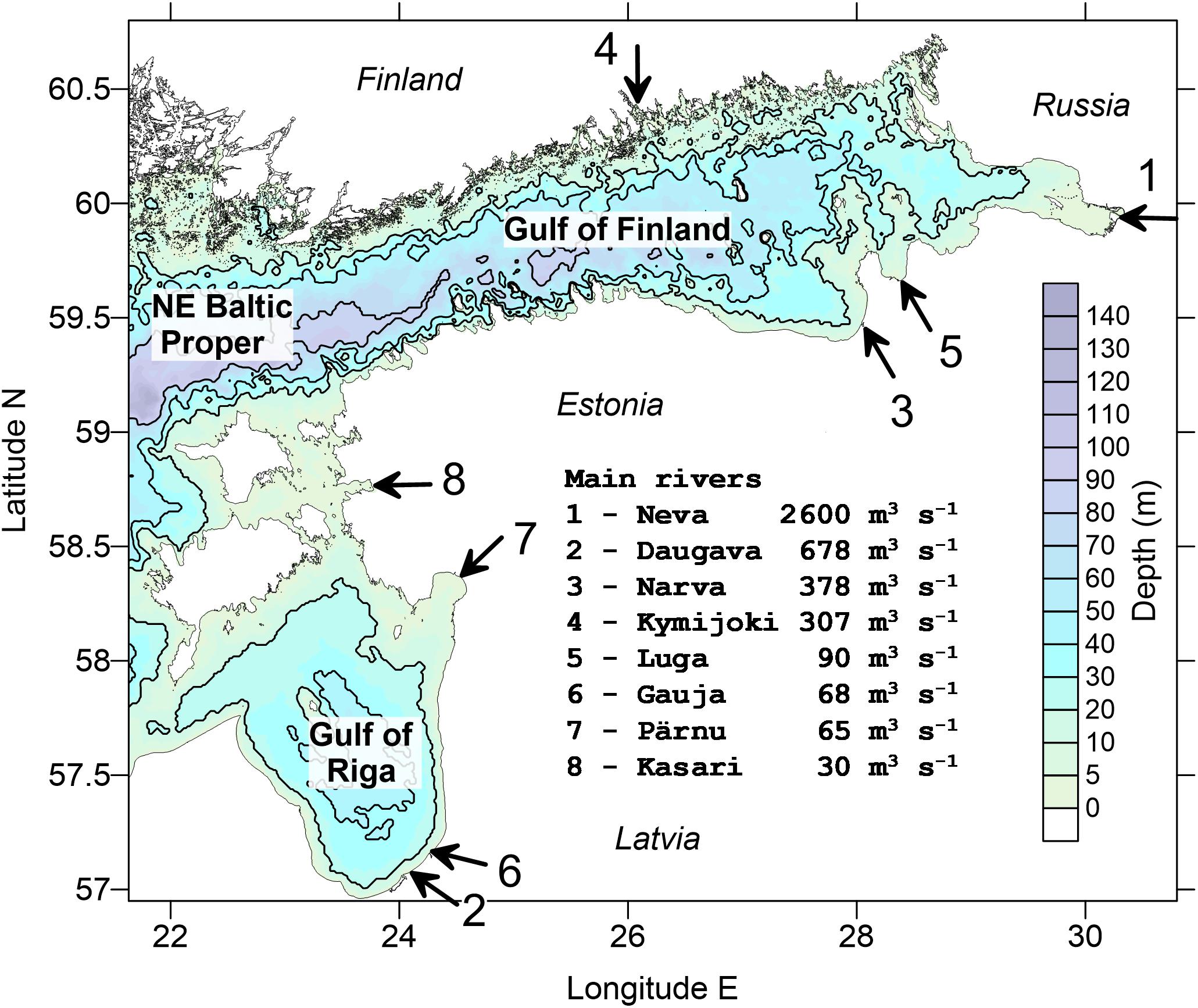
Figure 1. A map of the study area in the northeastern Baltic. Shown are the main 8 rivers bringing into the sea mean freshwater discharge (m3 s–1) as given in the legend.
We used the HBM model (Berg and Poulsen, 2012) with sub-regional 0.5 NM (nautical mile, 926 m) setup (Lagemaa, 2012; Zujev and Elken, 2018) in the geographical bounds shown in Figure 1 to produce the SST and SSS data. This HBM-EST model domain contains 529 × 455 horizontal grid points. Forcing at the western open boundary is taken from the Baltic-wide HBM model, which operates routinely within the Copernicus Marine Environment Monitoring Service (CMEMS) with the resolution of 1 nautical mile. Forcing on the sea surface is obtained from the Estonian version of the HIRLAM model that is run by the national weather service for operational forecasts on 11-km grid.
HBM is a 3D oceanographic model for the North and Baltic Sea, which uses Arakawa C-grid and is forced by surface energy fluxes (mechanical, radiative, thermodynamic) using bulk parameterization formulae. The model includes sub-models for turbulence parameterization. A model for ice thermodynamics and ice mechanics is embedded into the model system. The HBM model has been upgraded within the CMEMS from earlier BSHCmod versions. The Baltic-wide HBM setup is extensively validated within CMEMS. The quality information document for physical variables can be found on the web http://cmems-resources.cls.fr/documents/QUID/CMEMS-BAL-QUID-003-006.pdf as accessed on 10 July 2019.
For the analysis we used daily model data of free run (without data assimilation) averaged over 10 × 10 grid points, resulting in 744 wet points with 5 NM (9.26 km) resolution on the coarse grid. Since the grid step of the averaged fields is larger than the Rossby deformation radius, mesoscale patterns were suppressed in the analysis results. The 5-year analysis period covered 1826 dates from July 1, 2010 to June 30, 2015.
In the observational data we focused on the in situ SST and SSS data and remotely sensed SST data were occasionally used for the comparison. Shipborne profile observations were acquired from HELCOM/ICES database, downloaded from https://ocean.ices.dk/helcom/ on 12 February 2018. After extraction of surface data within the study area, 2915 data records were retrieved within 2009-2014. Prior to using the data for the reconstruction, oversampling for each particular time instance was eliminated by taking averages on the coarse grid and selected time interval. CMEMS remote sensing SST Level 4 (L4) data were downloaded from the service portfolio http://marine.copernicus.eu/services-portfolio/access-to-products/ as the product SST_BAL_SST_L4_NRT_OBSERVATIONS_010 _007_b. FerryBox data were obtained from the same portfolio as the product INSITU_BAL_NRT_OBSERVATIONS_013_032. Climatological monthly temperature and salinity fields were adopted from the study made by Janssen et al. (1999), covering the period 1900–1996.
Results
Mean and Standard Deviations of SST and SSS
The mean fields of surface temperature and salinity, shown in Figures 2A,B, were calculated as temporal mean values of individual grid points over the whole study period. Data assimilation was not performed; therefore, the presented maps may include some model bias. Primary purpose of the mean fields is to set the background for the variability study, i.e., investigate statistical properties of SST and SSS deviations from their fields.
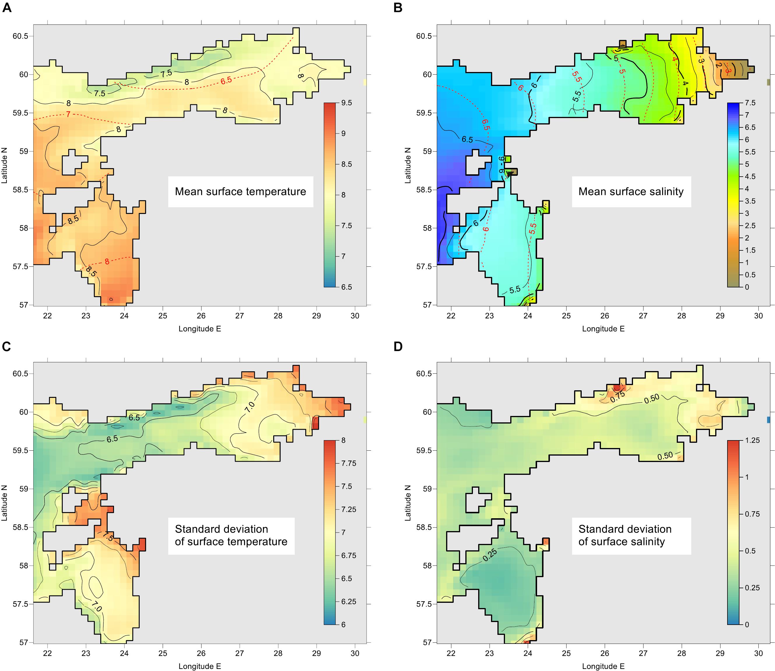
Figure 2. Maps of mean values (A,B) and standard deviations (C,D) for SST (A,C) and SSS (B,D). Model grid statistics is calculated from 1 July 1 2010 to 30 June 2015. Climatological mean values for the period 1900–1996 (Janssen et al., 1999) are shown in (A,B) by red isolines. The units are °C for SST and g kg–1 for SSS.
The maps of mean SST and SSS are dependent on the average atmospheric conditions during the period summer 2010 – summer 2015. The period covered severe ice winter (2010/2011), and average (2011/2012, 2012/2013) and mild (2013/2014, 2014/2015) winters (FMI, 2018). The mean SST map reveals lower temperature along the Finnish coast; that occurs during dominating westerly winds favoring upwelling in that region. This is consistent with mean salinity distribution in the Gulf of Finland that exhibited pattern typical to the dominance of reversed estuarine circulation (Westerlund et al., 2019), where tongue of less saline water near the Finnish coast is not present. While our SSS map is close to the yearly climatological map (Janssen et al., 1999) then SST is in the Gulf of Finland higher by 1–1.5°C and in the Gulf of Riga by 0.5–1°C.
Based on all the model values for the period 2010–2015, we calculated total mean value and the corresponding standard deviation σ for SST as 8.2 and 7.0°C, and for SSS as 5.45 and 1.3 g kg–1. While variability of SST is strongly dominated by temporal changes, SSS variability reveals dominant spatial changes. Namely, mean temporal variance , calculated on the basis of all spatial points k, comprises 99% of total variance for SST but only 11% for SSS. The remaining percentage of variance is due to variability of spatial means. Alternatively, mean spatial variance , calculated on the basis of all temporal instances i, reveals 97% of total variance of SSS and only 3% of SST. During individual time instances, spatial standard deviation σx(i) for SST was found from 0.08 (during winter) to 2.8°C; SSS values range from 0.95 to 1.5 g kg–1.
Maps of temporal standard deviations σt(k), calculated for each spatial point k, are presented in Figures 2C,D. These maps include seasonal cycle but also interannual and shorter period variations. Despite the small fraction of spatial variance of SST, some distinct spatial features over the area are evident. Higher temporal standard deviations of SST (above 7.2°C) are found in the shallow areas in the eastern part of the Gulf of Finland and in the Moonsund located between the large Estonian islands and the mainland. Spatial variations σt(k) of SSS are in the range from 0.14 g kg–1 to 1.5 g kg–1 (Figure 2D), whereas higher values occur near the entrance of larger rivers. High spatial variations of standard deviation make difficult using spatial correlation functions, which calculation require normalizing covariance with variance.
Covariance and EOF Characteristics
We calculated SST and SSS covariance according to Equation (3). After EOF decomposition of B using Equation (2), we also calculated covariance of the sum of six most energetic modes and of the rest higher modes. Due to orthogonality, covariance is additive regarding the EOF modes, i.e., the full covariance is the sum of covariance of the component data sets (six most energetic modes, and the rest higher modes). In Figure 3 SST and SSS covariance are presented as a function of space lag between the model points. We see significant spreading of individual values of covariance over pairs of points and conclude that calculated covariance is not homogeneous, which is usually assumed in implementation of OI.
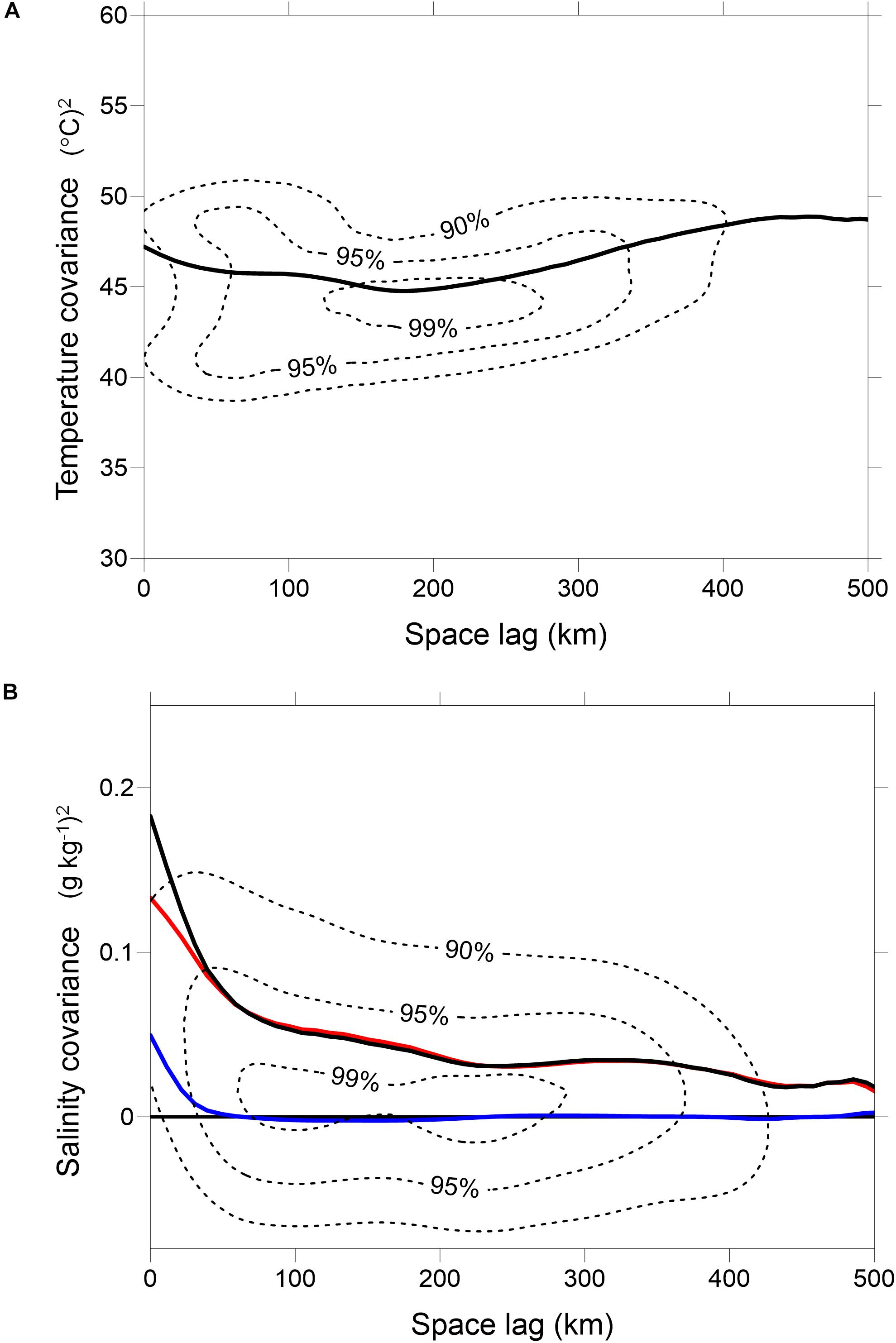
Figure 3. Covariance of SST (A) and SSS (B) as a function of space lag between the model points. Shown are heavily smoothed two-dimensional relative histograms of the original data (dotted lines, percentiles 90, 95, and 99%) and mean covariance of original data (black line). For SSS are shown also covariance of the sum of six most energetic EOF modes (red line) and of higher EOF modes (blue line). For SST the latter curves are not distinguishable from mean covariance and zero, respectively.
In the bins of space lags, distribution (histogram) of covariance of original fields and of the sum of most energetic EOF modes (not shown) usually does not follow the normal distribution. Therefore, mean covariance values can be considered only as indicative, since they differ significantly from the median values. Still it is clear that big covariance values occur over large distances, especially for SST. Covariance of residual fields (sum of higher EOF modes) has a good normal distribution and it decays fast with increasing space lag. Correlation (not shown) goes below 0.2 at a distance of 30 km for both SST and SSS, justifying the use of OI for this part of the variability.
Spatial EOF mode patterns for 4 leading modes are given in Figures 4, 5 for SST and SSS, respectively. The one-dimensional vectors ek of the SST and SSS modes are remapped back into the two-dimensional geographical framework.
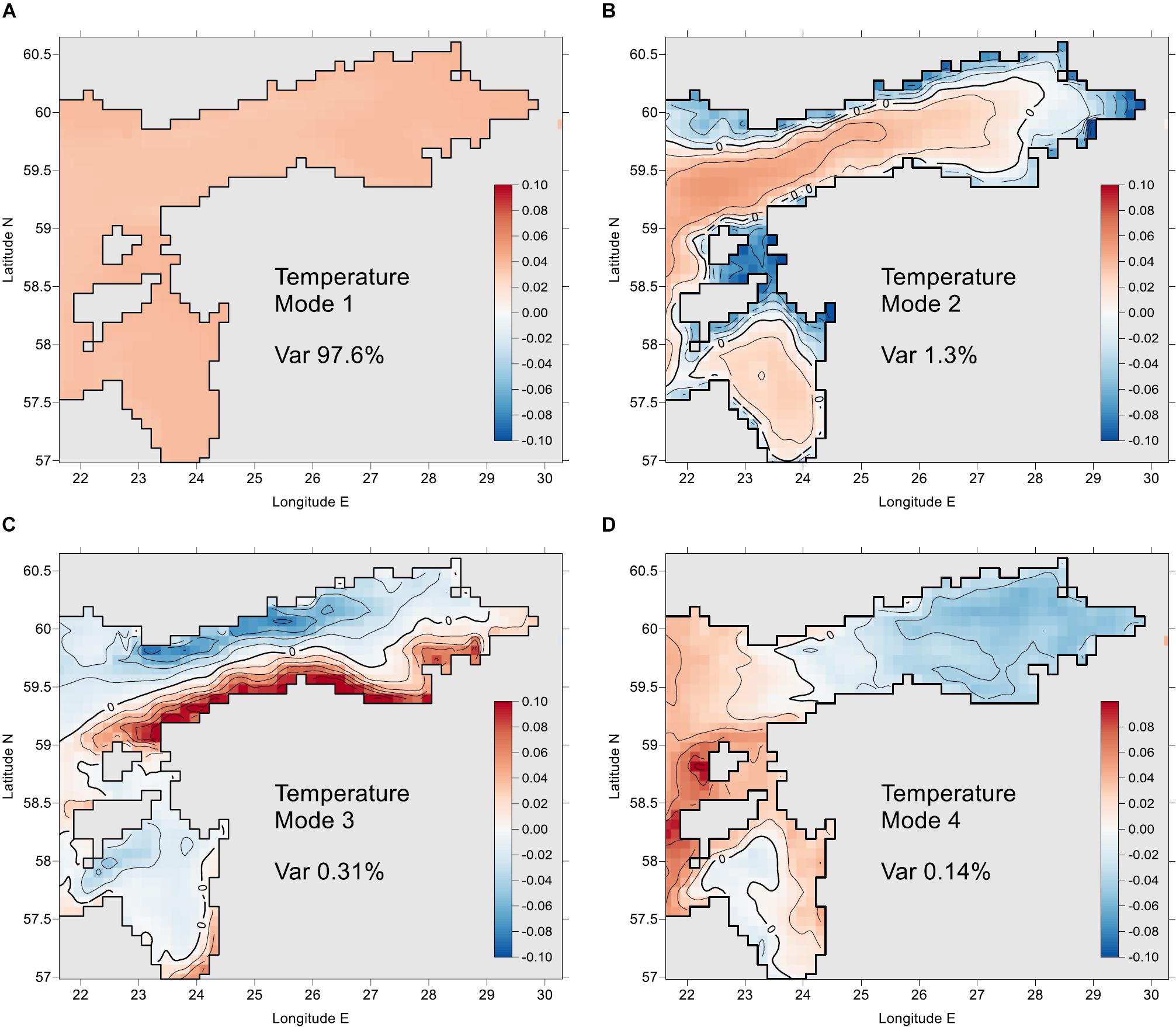
Figure 4. EOF patterns for four first modes of SST. Shown are the number of mode (1 to 4 as A to D) and explained variance percentage of each mode. Contour interval for non-dimensional normalized modes (744 points) is 0.02.
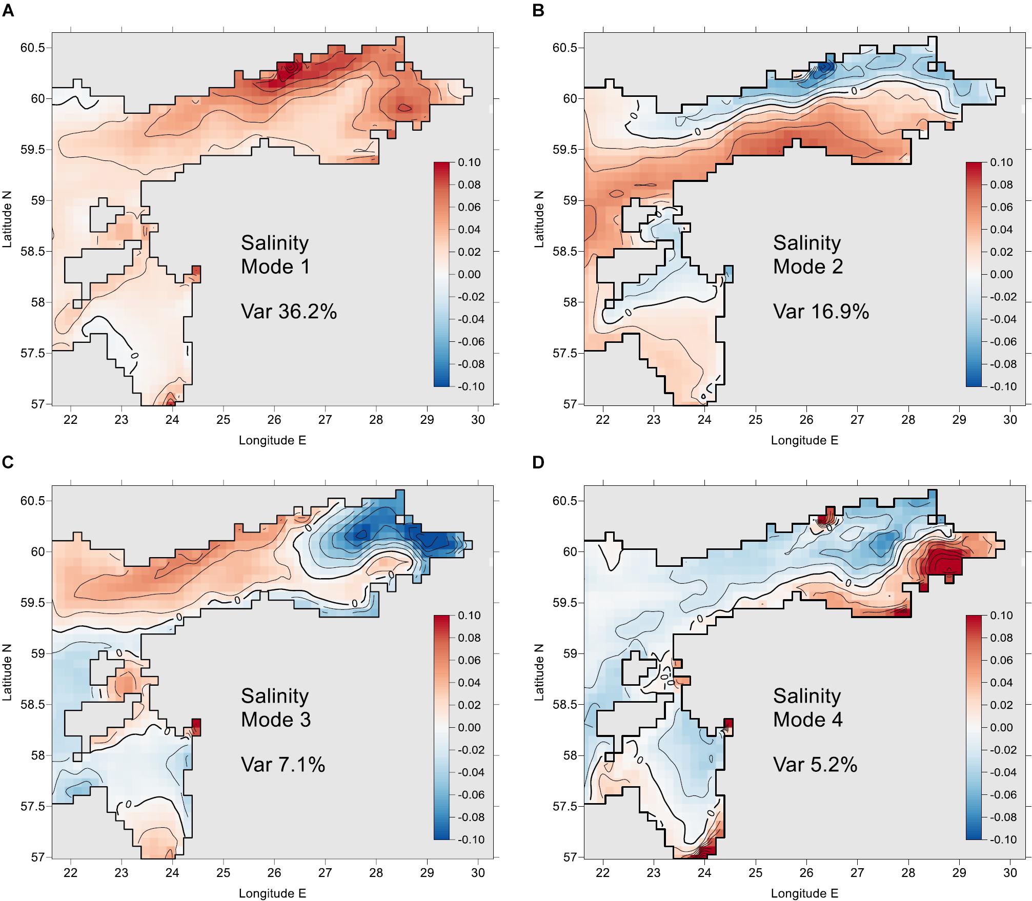
Figure 5. EOF patterns for four first modes of SSS. Shown are the number of mode (1 to 4 as A to D) and explained variance percentage of each mode. Contour interval for non-dimensional normalized modes (744 points) is 0.02.
Among the spatial patterns, large-scale physical interpretation can be easily found for four to six modes. The first, most energetic modes have nearly “flat” patterns without sign change; their amplitudes are dominated by a seasonal signal. Higher modes are considered random due to eddies and other mesoscale processes, therefore their correlation decays rapidly with increasing distance (see the earlier sub-chapter). In the SST patterns, the first mode dominates heavily (97.64% of variance explained) due to the seasonal cycle (Table 1). In the SSS patterns (Table 2), the share of different modes is more distributed and the first six modes explain 72.88% of the total variance.
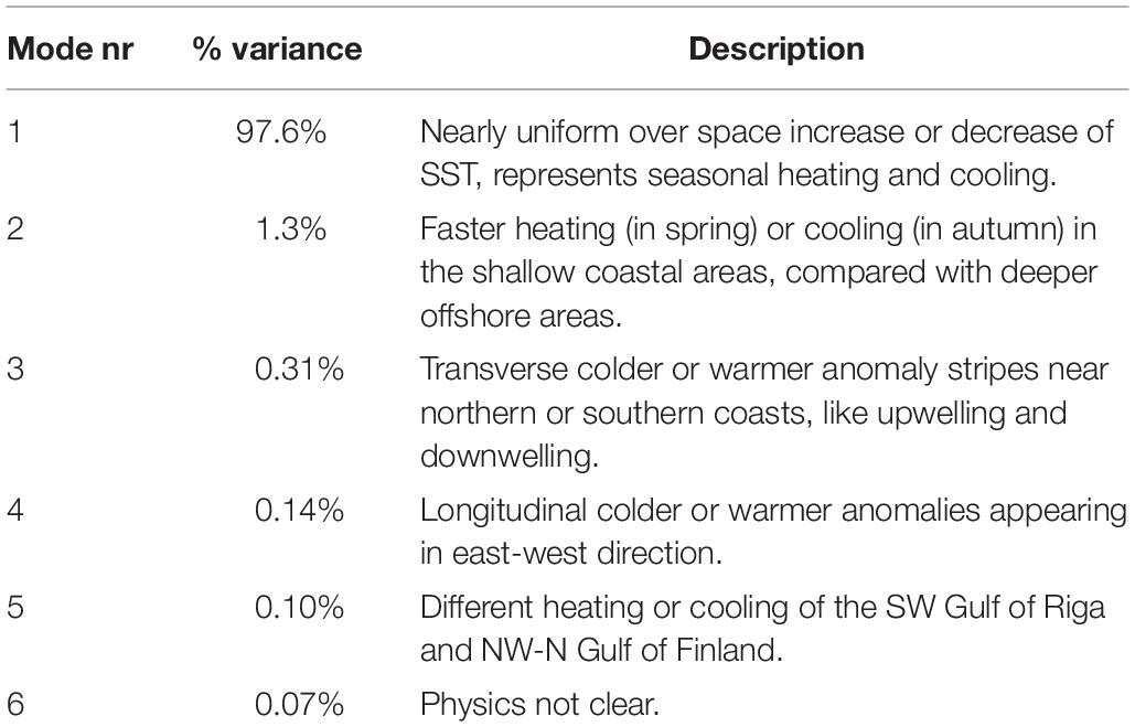
Table 1. Characteristics of SST modes.
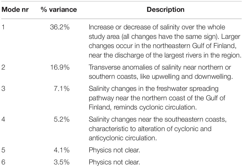
Table 2. Characteristics of SSS modes.
Temporal variance of the mode amplitudes equals to the eigenvalues of covariance matrix B. Based on the statistical features of the amplitudes, it is possible to set the “natural” limit Fk for each of the mode k. During EOF reconstruction, we use only the modes k where the estimated individual amplitude values at time i follow the condition . Since the absolute values depend on the number of grid point, configuration of the sea area and other factors, we do not present the numerical values of Fk. Excluding 10% of the higher and lower values of “natural” (calculated from full set of model results) amplitudes, a reasonable limit is .
We have presented in this paper the formulae (5)-(7) how to reconstruct gridded fields from observations made during one fixed time instance. Actual spatial observations are quite often not instantaneous in time. The weights of observations from past and future times depend on the temporal covariances (or correlations). Within the EOF decomposition, amplitudes of SST and SSS modes have different temporal correlation patterns, as shown in Figure 6. For the SST, the first and the second modes are nearly annually periodic with correlation r > 0.9 and shifted phases. Moderate semi-annual periodicity (r∼0.2–0.3) appears on the fifth mode. The first SSS mode has annual harmonic with r≈ 0.4. The second SSS mode has even stronger annual harmonic with r≈ 0.6. Based on long correlation times, we consider the method of EOF reconstruction of time-dependent observations, presented by formulae (8)-(9), justified for the time window up to 1–2 months.
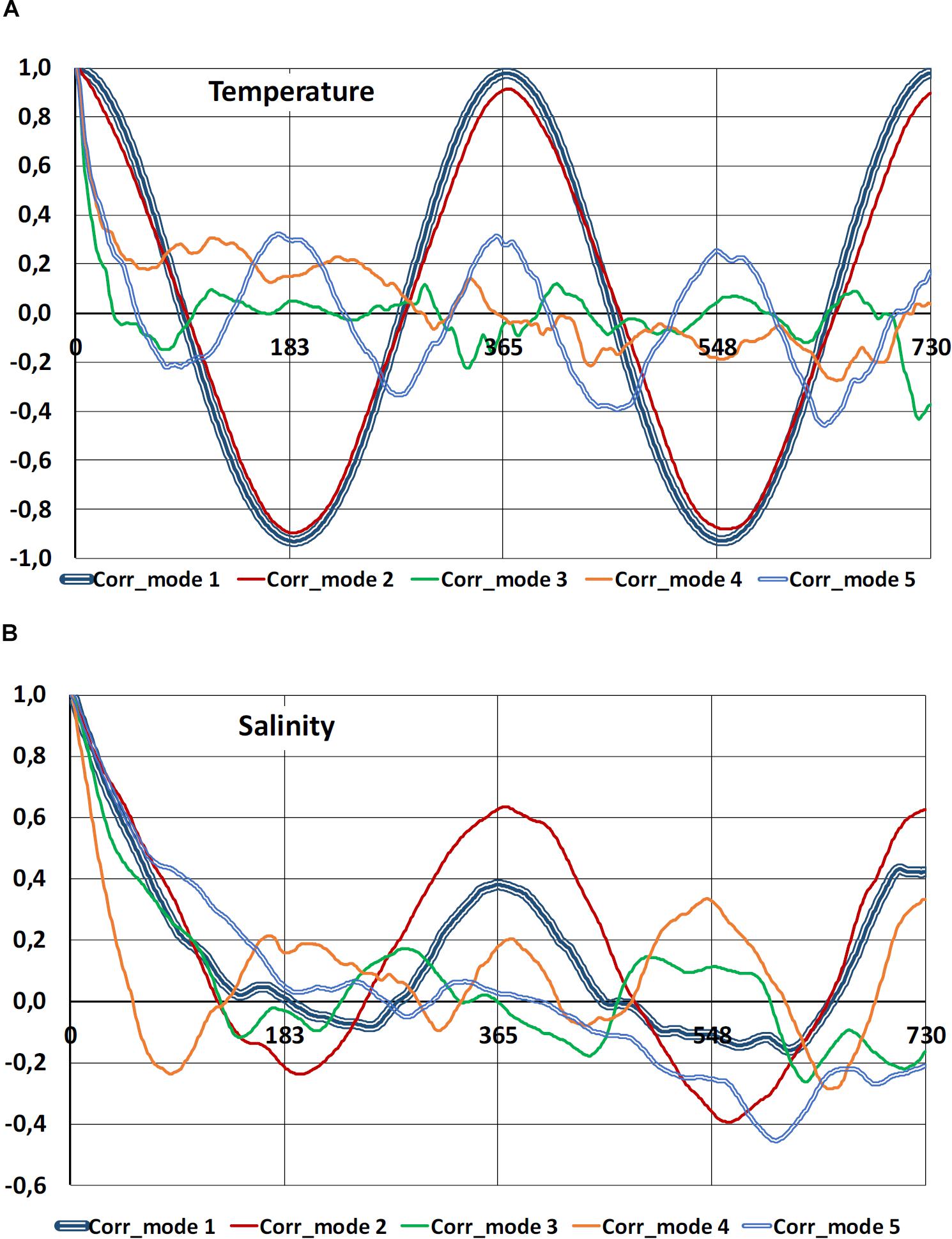
Figure 6. Temporal correlation functions of first five EOF mode amplitudes given in the legend for SST (A) and SSS (B). Horizontal axis shows time lag in days.
Reconstruction Errors: Experiments With Pseudo-Observations
Dependence of accuracy of EOF reconstruction on the number and spacing of observation points was firstly studied by grid configuration of pseudo-observations (see section Estimation of Reconstruction Accuracy Using Pseudo-Observations) with variable grid step. At prescribed locations, model data were extracted on specific time instance; then the result of gridded reconstruction was compared with the original model data. Observational grid step Δo was taken as integer n times the model grid step Δm, Δo = nΔm. Observation grid step factor n was cycled from 1 (observations taken at all the model points) to 11 or more (leaving 2-6 observation points).
We made pointwise comparison of all the 744 spatial points during 1826 time instances, using 6 EOF modes for the reconstruction. Frequency histograms of deviations for SST and SSS are presented in Figure 7 for two spacing options between the pseudo-observations. We reveal that error histograms are quite insensitive to the number of observations K, when it is larger than the number of significant modes L. However, at small observation amounts the number of larger errors (can be considered as outliers regarding normal distribution) increases. On the background of grid points of 37 km spacing, reconstructed SST and SSS maps are shown for one arbitrary date 19 June 2015 (Figures 8C,D) together with the original model data (Figures 8A,B).
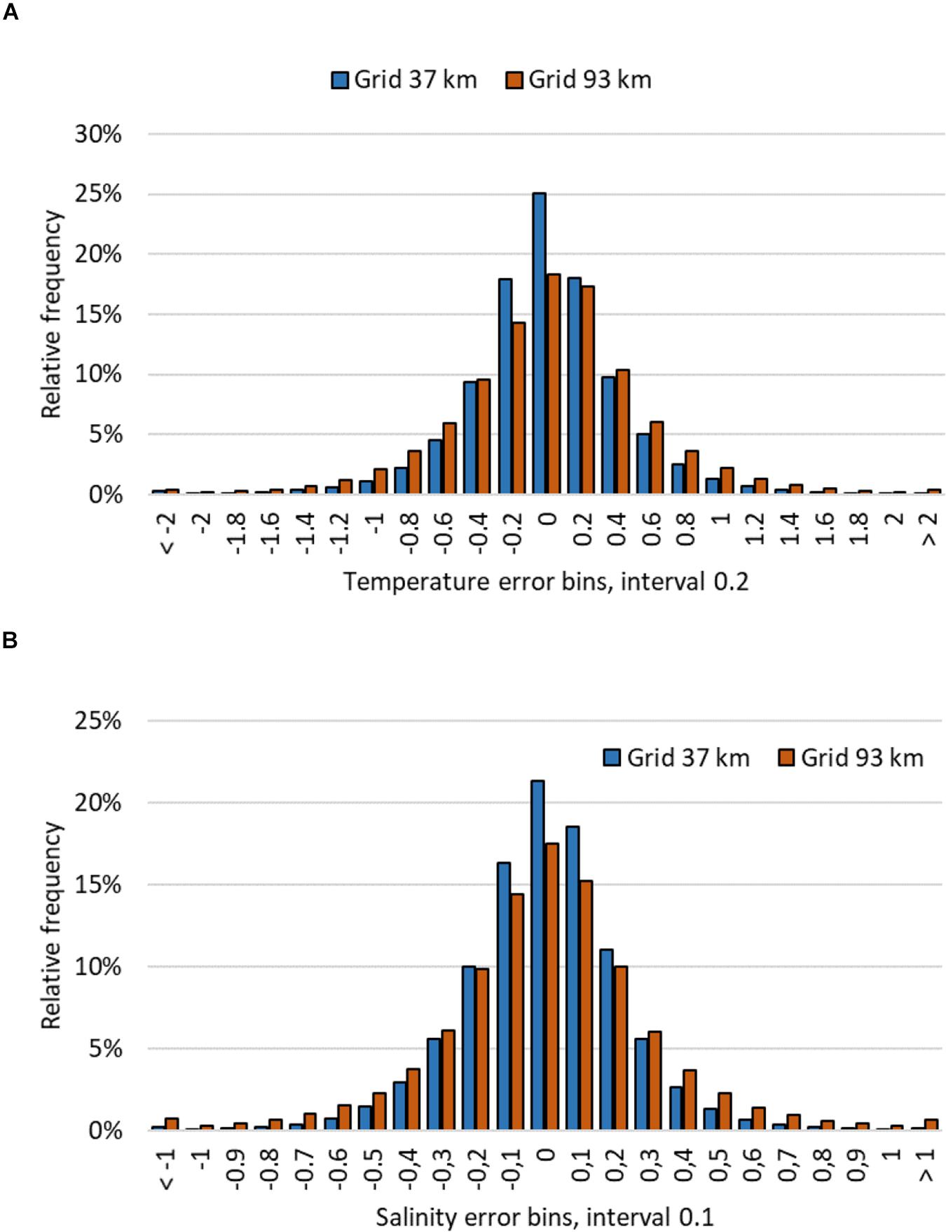
Figure 7. Relative frequency of SST (A) and SSS (B) differences between reconstructed (sum of six EOF modes) and initial field. Shown are results with pseudo-observation data prescribed by 37 km grid step (51 observation points) and 93 km grid step (10 points). Compared are about million data pairs.
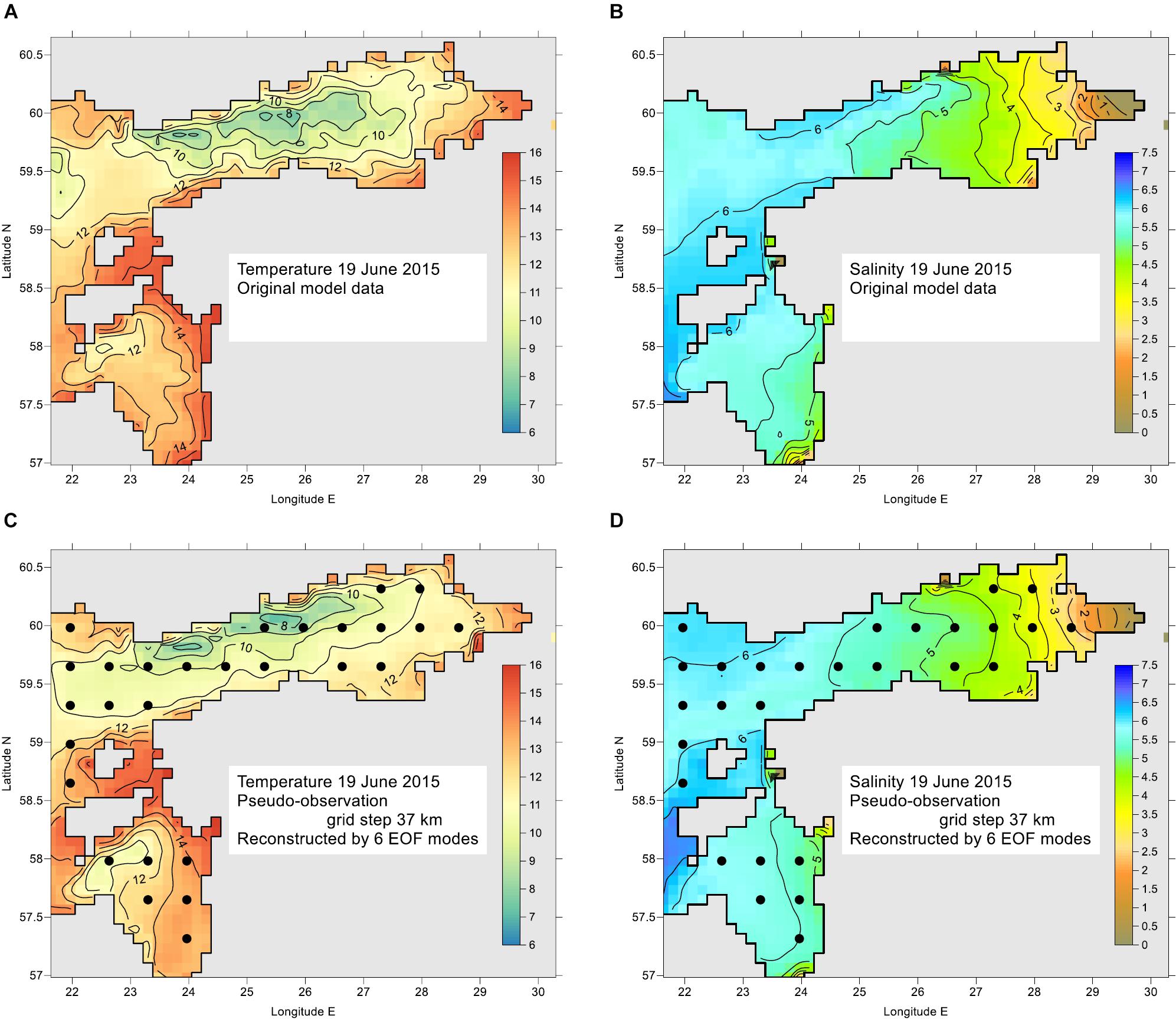
Figure 8. Snapshot of original model data on 19 June 2015 for SST (A) and SSS (B) and corresponding reconstructed maps (C,D) using pseudo-observations from a grid with 37 km step shown by dots. Reconstruction was made by 6 gravest EOF modes. The units are °C for SST and g kg–1 for SSS.
With decreasing number of observations K, errors slightly increase when still K > L. For example, SSS absolute error is less than 0.3 g kg–1 for 88% of cases with K = 51 and 80% of cases with K = 10. Regarding SST, the errors are less than 0.6°C correspondingly for 90 and 82% cases. Regression of all the values of both SST and SSS yields tangent between initial and reconstructed data 0.99, their correlations follow r > 0.95. Relative errors of all the SST data, compared with horizontal standard deviation σx(i) of each time instance, are from 6.7% (observation grid step 37 km) to 8.6% (93 km). Relative errors of SSS are somewhat larger, correspondingly 18 and 25%. For K < L the errors increase abruptly and singularity errors may occur in Equations (5)–(7).
Reconstruction capability from realistic sampling schemes was evaluated for typical monitoring network (with smaller number of stations than usual) and for two routes of FerryBox along Tallinn-Helsinki and Tallinn–Stockholm (Petersen, 2014; Kikas and Lips, 2016). Pseudo-observations from the selected configurations were run through all the daily model maps. The error statistics did not differ much from that of the above-described observation grid experiments. Inspecting the reconstructed maps (not shown), even with small number of observations the reconstructed maps generally match well to the original maps. The monitoring type of stations has observations in all the three main areas: Gulf of Finland, Gulf of Riga and adjacent Baltic Proper. The SST and SSS maps reconstructed from the pseudo-observations (not shown) match well the original maps. FerryBox data set has no data in the eastern Gulf of Finland and in the Gulf of Riga (see an example by Elken et al., 2018), therefore larger deviations of reconstructed data from initial data occur in these regions. However, main large-scale SST and SSS features, present in the initial model data, can be identified in the reconstructed maps rather well.
For comparison of EOF reconstruction with OI, we set up an experiment where EOF statistics were calculated during 4 years from 1 July 2010 to 30 June 2014, and the remaining 1 year period from 1 July 2014 to 30 June 2015 was dedicated for comparison. For each set of Δo = nΔm, we included all the possible shifts of observation grid into the comparison. For example, in case of n = 8 there are 64 options for grid shift. All those shift options produce different result of reconstruction, because of different resolution of topographic and coastline features and freshwater input areas. The points just neighboring the coast were excluded. The method of OI was used with correlation scale R = 200 km and noise-to-signal ratio η2 = 0.1 (see section Estimation of Reconstruction Accuracy Using Pseudo-Observations).
Dependence of RMSD of reconstruction on the spacing for 3 compared methods – EOF, OI-M with modeled mean field, and OI-C with climatological mean fields – is presented in Figure 9 as median values taken over all shift options. The spread of individual shift estimates increases from the spacing 46 km toward greater spacing and smaller number of pseudo-observations, especially for the EOF method. In case of SST, EOF methods produces on the average more accurate reconstruction than both of the OI methods using the values given above. Still, during individual time instances the reconstruction results may have similar difference pattern at large spacing of sampling (Figures 10A,C) since coastal features may remain unresolved. We had to choose large correlation scale and noise-to signal ratio in order to have reconstruction over the whole area even if the spacing of observations is large; then OI tends to make heavy smoothing that is reflected in Figure 9A by larger RMSD. SSS field is dominated by spatial variations; one control value of such domination is RMSD = 0.411 g kg–1 of “no observations” (at each grid point, mean value is taken instead of observed value) that lies in the range of RMSD variation (Figure 9B). Evaluation reveals that EOF reconstruction has slightly larger error than OI relative to the modeled mean field. Commonly used OI with deviations from climatological mean reveals larger RMSD than EOF; it even exceeds the “no observations” already with spacing larger than 28 km. These features of RMSD appear due to the specific topographic and hydrographic features of the region: fragmented coastline and prevalence of low-salinity regions with surrounding higher spatial gradients and temporal standard deviations (Figure 2) near the entrances of larger rivers (Figure 1). If OI considers and interpolates the SSS deviations from highly variable spatial mean map (determined by the model that resolves local features), then such deviations follow normal distribution without significant outliers (not shown) and local features appear in the reconstruction product without remarkable distortion. Deviations from spatially smooth climatological mean values (Figure 2B) contain a high number of outliers to the normal distribution, that cause larger distortions of OI-C reconstruction in the river influence areas than EOF reconstruction (Figures 10B,D).
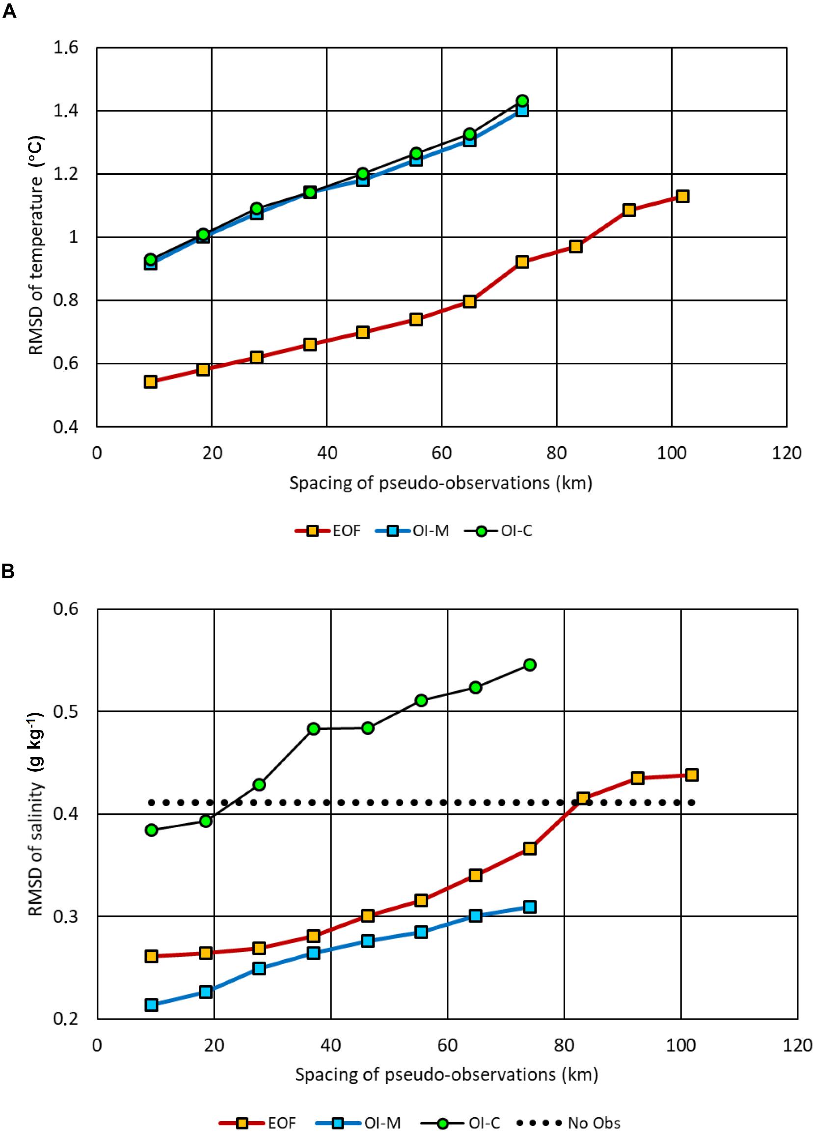
Figure 9. Dependence of RMSD between reconstructed from pseudo-observations fields and original model output fields of SST (A) and SSS (B) for different methods: EOF, reconstruction by 6 gravest modes; OI-M, optimal interpolation with modeled mean field; OI-C, optimal interpolation with climatological mean field. The grid step of pseudo-observations cycled from 1 to 11 model grid steps, all possible shifted configurations of off-shore stations were taken into account. Median values of RMSD are presented. “No Obs” means the spatial standard deviation of temporal mean values.
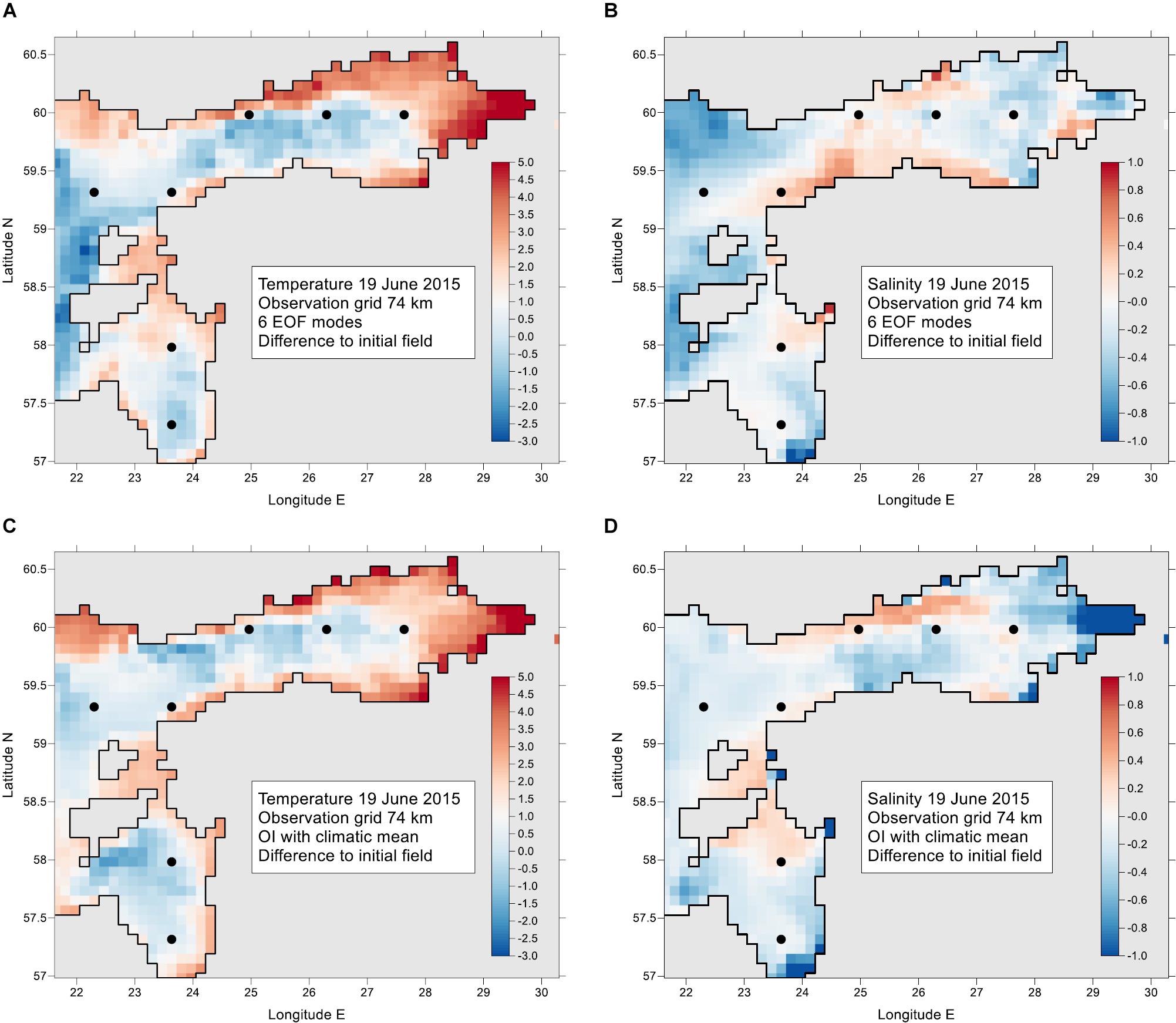
Figure 10. Snapshot of differences between original model data and reconstructed data on 19 June 2015 for SST (A,C) and SSS (B,D). Pseudo-observations were taken from a grid with 74 km step shown by dots. Reconstruction was made by 6 gravest EOF modes (A,B) and by OI using the deviations from climatological mean (C,D). The units are °C for SST and g kg–1 for SSS.
Seasonality Issues in EOF Reconstruction of SST
Among variety of physical processes, original SST data from model reveal significant seasonal variation in time. Annual cycle is evident in temporal correlation of the amplitudes of first and second EOF mode (Figure 6) that cover 98.9% of total variance. This cycle is slightly variable in space, whereas highest spatial variations (not shown) occur during the spring heating period and smallest variations take place in the winter when SST is close to or equal to freezing temperature.
It is interesting to consider what will happen to the EOF reconstruction results when seasonal signal is removed from space-time matrix X prior to the procedures by Equations (1)–(7). Following Høyer and She (2007), we introduce a modified data set where time slices of spatial data with seasonality removed are defined at time index i as
where seasonal data si are evaluated in each model grid point k. Consider a time series vector xk which values are available on times ti counted as fractions of decimal year. Based on the total M data of xk(ti), make an approximation of seasonal cycle by a biharmonic function
The coefficients from C1,k to C5,k are found to obtain best fit of sk(ti) to the values xk(ti)in terms of minimizing their RMSD. The fitting coefficients and resulting seasonal cycle are spatially variable, whereas earlier and higher SST maxima generally appear in shallower coastal waters.
Overall variance of SST, determined in reference to the constant mean value, was 47.35 (°C)2 whereas spatial variability due to temporally constant mean values in each grid point covered 0.3%. By introducing the seasonal cycle removal procedure by Equations (10)–(11), variance percentage of the input field for the EOF analysis was significantly reduced: from 99.7% for xi to 6.1% for . The fitting biharmonic seasonal cycle contained 80.0% of total variance and the remaining 13.8% appeared in the covariance between and si.
Although variability of was reduced as compared with xi, spatially mean deviation from the seasonal cycle was typically in the range from −2°C (mostly in autumn) to +4°C (in summer). Spatial standard deviations of had maximum values during summer, amounting typically to 2.5°C. Wintertime minimum of spatial standard deviation, apparent in the initial xi data, was not anymore apparent since biharmonic sk(ti) had in winter problems to follow the constant level of freezing temperature.
Spatial covariance estimates of (not shown) reveal significant similarity to the estimates based on the original data xi (Figure 3A): covariance at distances of several hundreds of kilometers is close to the covariance at zero lag since significant part of SST variability is caused by weather events and interannual variations that occur nearly uniformly over smaller sub-regions like in our case. Based on the full covariance matrix, EOF analysis revealed highly similar patterns of leading modes of to the modes of xi which are shown in Figure 4. The share of “flat” first mode (Figure 4A) decreased from 97.6 to 80.5% after removal of biharmonic seasonal cycle. At the same time, the shares of higher modes 2–6 increased from 1.91 to 12.79%. In addition, the second and third mode changed their order and the “upwelling” mode (Figure 4C for xi) got a bit higher share of variance as the “differential heating” mode (Figure 4B for xi) since those variations were already partly included into the spatially variable seasonal cycle.
The original model field X can be approximated by leading EOF modes using equation (1), whereas the higher eigenvectors are truncated to zero. Using six leading modes both for xi and datasets, the decompositions seem highly similar. However, evaluation of RMSD allowed detecting of 4% reduction when seasonal cycle was removed prior to the EOF procedures.
When there are much less observations than the number of grid points, reconstruction accuracy can be estimated using the pseudo-observations method. Example of comparison of the two datasets is presented in Figure 11, based on the “observation” data that were extracted in seven locations shown in Figure 10. The reconstruction errors were correlated with r = 0.71, whereas the regression line was (errors of ) = 0.965 (errors of xi). Both reconstructions had very high correlation with the initial model data r > 0.99 and the scatterplot graphs (not shown) created the impression that the data sets were nearly identical. Actually, already small variations in the correlation modify RMSD and in case of our example, there can be about 25% of RMSD reduction when seasonality is removed prior to the EOF analysis.
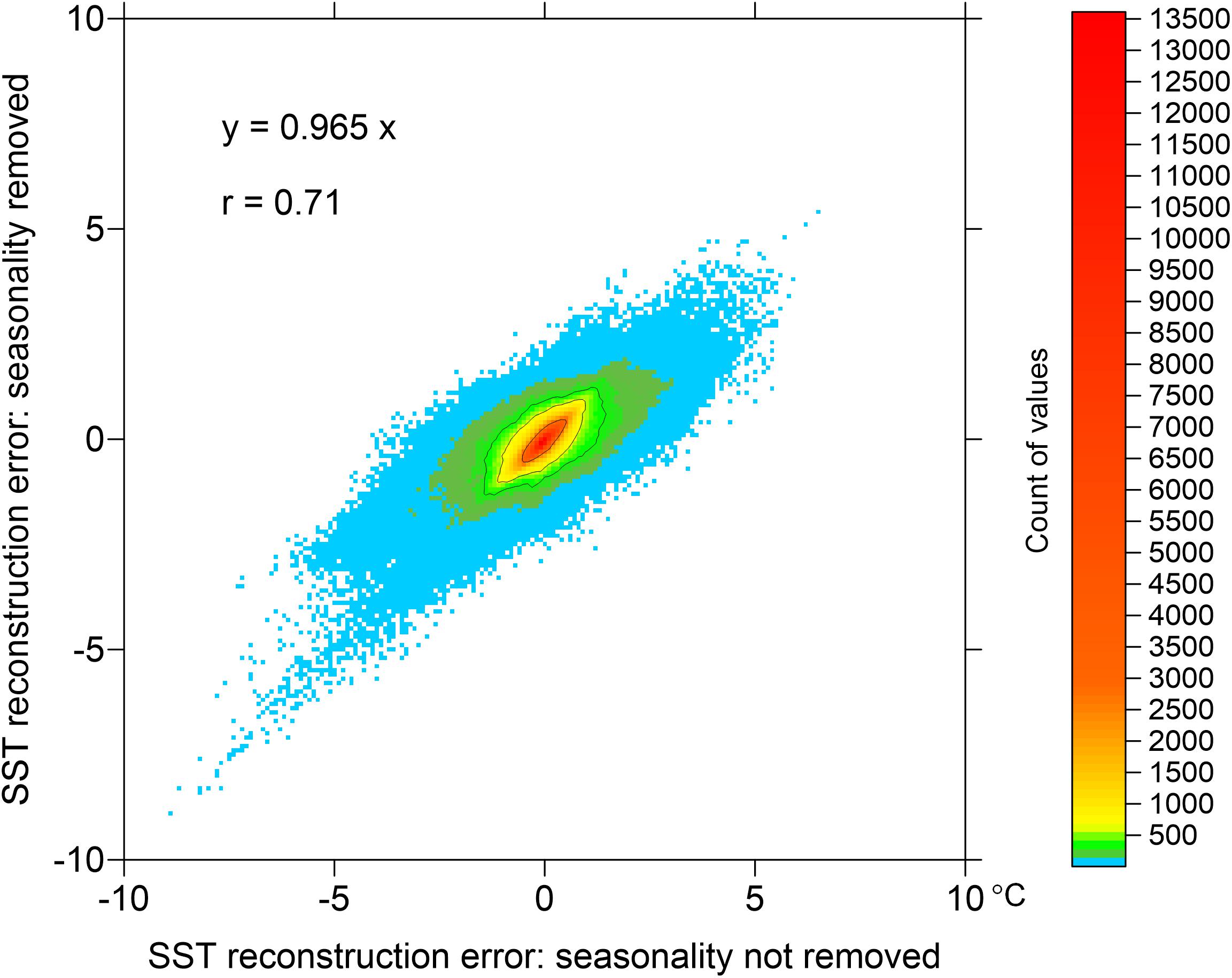
Figure 11. Two-dimensional histogram of reconstruction errors within the experiment with pseudo-observations on the observation grid 74 km as shown in Figure 10. Compared are 678,528 values of reconstruction error in reference to original model data. Reconstruction was based on six EOF modes using the original approach where seasonality was not a priori removed (abscissa) and the modified approach where biharmonic seasonality was removed prior to EOF analysis (ordinate). Solid lines represent 90, 95, and 99% percentiles.
Splitting the Region Into Sub-Areas
In one of the experiments, the whole region presented in Figure 1, was split in three sub-regions: Gulf of Finland (GOF), Gulf of Riga (GOR), and NE Baltic Proper (NEBP). Individual EOF modes were calculated for each of the sub-area. Except for NEBP, the first two SST modes for GOF and GOR were similar to the patterns obtained for the whole area. Pairwise correlations of the SST amplitudes were r > 0.95 between the GOF, GOR and the whole region. The whole region and GOR correlations for the first three SSS modes were r > 0.9 while the first mode of GOR correlated with GOF with r > 0.72 and with the whole region with r > 0.78. The first three modes of SSS of the whole region covered 61.4% of variance. The split regions had the mode coverage: GOF – 69.9%, GOR – 53.7%, NEBP – 72.8%. Although by splitting the region, mode convergence (share of variance of the lowest modes) increased slightly, we judged that EOFs of the whole region cover the regional dynamics in sufficient accuracy. Note, that region splitting may become important in other regions, where the mode convergence of the whole region might not be satisfactory.
Examples Using Actual Observations
Taking Into Account Time Dependence of Observations
It is usual practice, that spatial shipborne monitoring is carried out by different ships belonging to different institutes and countries. Covering the whole region may take quite long time. On an example, given in Figure 12, four ships with ICES codes 3499, 34AR, ESLV and LAVA made observations during 17 days from 18 May to 3 June 2009. During this spring heating period, SST generally increased from 7 to 15°C, but local SST variations were also evident. Over the time span, observations in the northern area were taken in the first part when water was not yet heated as much as by the end of the period. Considering the observations as instantaneous, reconstruction using Equations (5)–(7) provided rather cold waters there. In turn, warm waters were drawn in the coastal areas where observations were taken at the end of the period (Figure 12A). EOF reconstruction using the time dependence of observations based on Equations (8)–(9), setting the reference time in the middle of the period (Figure 12B), increased the temperature in the region of earlier observations and decreased in the region of later observations, reducing this way the artificial contrasts due to non-synchronous observations. Comparison with satellite based SST map from CMEMS L4 product (Figure 12C) reveals good similarity to the time-corrected map. Numerical differences are mostly less than 1°C, not exceeding the range of unresolved here diurnal oscillations (Karagali and Høyer, 2014). From the number of calculations we got the experience that reference time may be modified within the observational window without loosing the realism of reconstruction. However, extrapolation outside the window should be avoided like in the case of one-dimensional linear regression.
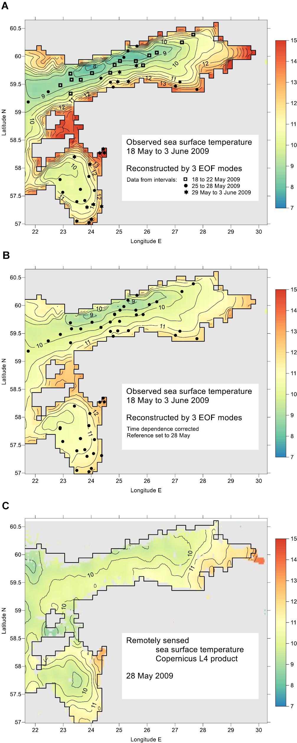
Figure 12. Reconstruction of sea surface temperature (°C) using data from ship observations during the spring warming period from 18 May to 3 June 2009. Locations of the data from the ICES database are shown by symbols presented in the legends. Reconstruction is made using the three leading EOF modes: (A) considering all non-synchronous data as instantaneous (see three time intervals in the legend), (B) introducing correction for time dependence, with reference set to 28 May. For comparison, daily mean SST L4 map determined by remote sensing from satellites is presented for 28 May 2009 (C).
Automatic Reconstruction of Time Series of Maps
It is technically easy to set up procedures for automatic reconstruction of time series of maps, using the time dependence of observations based on Equations (8)–(9). We took the shipborne profile data from ICES database (see section Regional Setting of Experiments).
During the reconstruction procedure, EOF amplitudes for each map were checked against the criteria (see section Covariance and EOF Characteristics) in order to determine the number of “good modes.” Taking the time window for one map 1/12 year (about 1 month) and the limit of at least 8 non-duplicate observations within the time window (time average was taken over 2 days), we obtained 148 maps for SST and 137 maps for SSS, out of maximum 209 maps. Average number of data points is 25 and maximum amounts to 83 both for SST and SSS. We note that large number of observation points does not necessarily mean high number of good EOF modes. For example, the observations with highest amount 83 were fragmentarily located along the coasts as short-scale repeated maps; the number of good modes was only 3. Good six modes were in other configuration obtained already from 20 to 30 observation points.
From reconstructed maps, SST and SSS time series were extracted around monitoring stations LL12 (western Gulf of Finland, 59.4835 N, 22.8968 E), V15 (Moonsund, 58.8167 N, 23.2167 E), G1 (central Gulf of Riga, 57.6167 N, 23.6167 E), K21 (Pärnu Bay, 58.2167 N, 24.3083 E), F3 (central Gulf of Finland, 59.8383 N, 24.8383 E) and LL3A (northeastern Gulf of Finland, 60.0672 N, 26.3467 E). Such reconstructed time series can be easily extended to climate studies.
Individual maps, reconstructed by the automatic procedure (example is given in Figure 13), follow closely the observed values but also reveal realistic patterns compared to the published knowledge on Baltic Sea climatology and monthly and instantaneous distributions (e.g., Leppäranta and Myrberg, 2009).
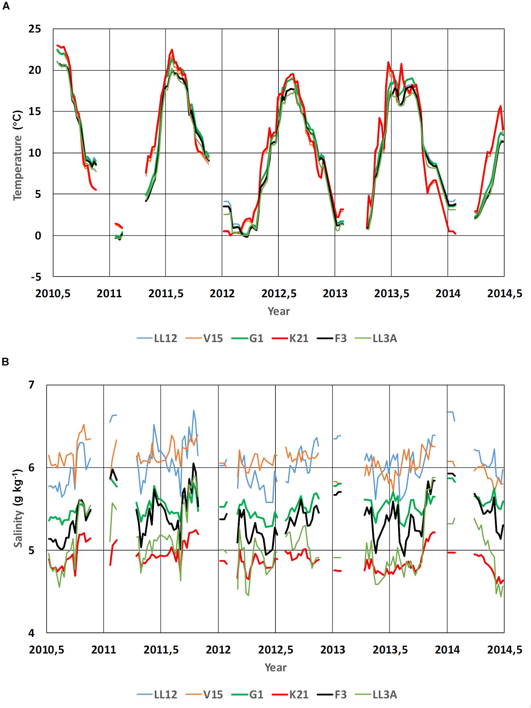
Figure 13. Time series of sea surface temperature (A) and salinity (B) reconstructed from the shipborne data downloaded from the ICES database. Reconstruction is made for six locations (LL12, V15, G1, K21, F3 and LL3A, see the text for locations) for the times from 2010.5 to 2014.5 with 1/24 year (15.33 days) interval. Time window for including the observations and evaluating the EOF amplitude rate of change was taken 1/12 years. Presented are the periods when at least 8 points occur within the time window. Number of good modes was chosen three, but time instances when the highest good mode was two were also included.
Discussion
There is a continued need for producing gap-free gridded oceanographic data using observations. Although new observation techniques became available, the problem of fragmentation remains in oceanographic data management. Reanalysis is a powerful, but costly method for production of gridded fields. Widespread statistically based methods like OI (optimal interpolation), DIVA (Data-Interpolating Variational Analysis, Troupin et al., 2010) etc. use mainly localized covariance patterns. Covariance estimates from models reveal large values over basin scales due to trends, seasonal signal and basin-wide dynamics (e.g., coherent upwelling-downwelling near opposite coasts). Such covariance estimates suggest using of methods that use full covariance fields. In this context, the classical EOF method is again gaining interest (e.g., Yang et al., 2017; Pilo et al., 2018), whereas the statistics of the studied field can be estimated from the model results. Amplitudes of EOF modes can be approximately estimated from the observational data set which dimension is much smaller than the number of model EOF mode grid points.
When using model data to create the EOF statistics, it is important to know how reliable the estimates of modes and amplitudes with respect to model uncertainties are. Thorough treatment of the above question cannot be found in the literature. However, on the sea surface, temperature and salinity results from different models are rather well validated by observations and the model-based covariance patterns can be considered trustful. As a common practice, modeled covariance have been used in data assimilation. Fu et al. (2011) compared covariance patterns from modeled SST and satellite SST, and found them agreeing well. CMEMS QUID report has presented validation of SSS against ferrybox data, showing that the SSS patterns were well simulated by the model. In deeper layers, however, there is usually larger spread between different model results.
While ocean data come from different platforms and observations are non-synchronous, taking into account the time dependence of observations is a challenge. Amplitudes of lowest EOF modes reveal distinct temporal correlation patterns, with time scale several months. This could be used to handle temporal gaps and/or non-synchronous data, if they lie within the temporal correlation scale. As a first step, we introduced linear correction to the EOF amplitude depending on the difference of observation time relative to reference time.
We have made comparison of the results from EOF reconstruction with the results from classical OI method. Our test region – NE Baltic – is characterized by fragmented coastline and highly variable topographic and hydrographic conditions. In such region the spatial changes of oceanographic variables may have quasi-permanent anomalies like low salinity near river influence areas or faster warming and cooling in shallow coastal areas, compared to the offshore SST variations. Therefore, EOF reconstruction has a potential to achieve comparable or better accuracy than OI method.
EOF modes and amplitudes depend on the selection of domain. We used a sub-region, containing two geographical regions and their transition area. It was found that some of the modes (mainly the first mode) do not change significantly when the domain is separated into smaller parts. If the convergence of leading EOF modes of large sea area is low (share of explained variance is small), refinement into smaller areas might be useful. In our example, the convergence improved only slightly when partition into three smaller areas was made. Workable criteria for the region selection is not yet established, although following geographical regions seems to be acceptable.
In case of data assimilation into the high-resolution model, it is reasonable to separate low-resolution component and make large-scale corrections into that, keeping high-resolution deviation patterns unchanged. The workable approach for correction and/or assimilation of the data on the basin scales is as follows: (1) to separate the coarse-grid part from the fine grid data by spatial averaging, (2) to perform corrections on the smaller dimension coarse grid, (3) to interpolate coarse grid data back to the fine grid and add fine grid deviations determined from the interpolation of the initial coarse grid. This is based on the assumption, that correction of basin-scale features does not influence the mesoscale patterns, apparent on the fine grid but filtered out on the coarse grid. The EOF approach allows additional assimilation of mesoscale patterns in the regions of high data coverage.
We have tested reconstruction of SST and SSS in one sub-region of the Baltic, based on the in situ observations. The method itself allows to be applied on different data sets (for example, including high-resolution remotely sensed SST) of different variables and their combinations (for example, joint data vector of temperature and salinity), on the condition that significant part of variability can be presented by a few leading modes. There could be obvious extensions of the approach to cover the whole water column. This could be especially important to properly match the consequences of large salt water inflows etc.
One straightforward application of the approach could be in marine ecology, where building the gap-free patterns of nutrients and biomass variables could allow more precisely estimate the total amounts and budgets of ecosystem variables, and to evaluate the values of environmental indicators that are important for environmental management.
Conclusion
We have developed statistically justified EOF reconstruction method to handle large-scale patterns of observed fields in the sub-regions. The method uses model-based EOF patterns to interpolate and extend the observational data over the full study region. In the smaller sea regions, which are affected by the same large-scale forcing patterns, the EOF patterns have obvious physical interpretations and their shape does not depend very much on the selection of boundaries. When removing the SST seasonal cycle prior to EOF analysis, spatial patterns of leading modes remained practically unchanged, share of variance of the three first modes was reduced from 99 to 88.6% and reconstruction errors were reduced by about 25%.
Since we use only the first most energetic EOF modes, we can cover with this method basin and sub-basin scales of variability. The relative interpolation errors, estimated over the full area, usually remain below 10% for SST and 20% for SSS, compared with multi-year standard deviation of all variability relative to their mean value over the basin. In comparing with OI, EOF is especially useful for reconstruction with very sparse observations. In the regions of denser sampling, EOF cannot exactly follow the observations. Mesoscale deviations from large-scale EOF patterns follow well-defined covariance decay with space lag; therefore, they could be treated by optimal interpolation or similar method.
Author Contributions
All authors contributed in analysis and writing, with JE as lead author and JS making strong co-contribution. MZ made the EOF calculations while PL was in charge with the HBM model.
Funding
This study was supported by the Ph.D. program for MZ and the institutional research funding IUT 19-6 of the Estonian Ministry of Education and Research.
Conflict of Interest Statement
The authors declare that the research was conducted in the absence of any commercial or financial relationships that could be construed as a potential conflict of interest.
Acknowledgments
A larger BAL MFC team within the EU projects MyOcean, MyOcean2, and MyOcean-FO did the development of HBM model. This cooperation is highly acknowledged.
References
Alenius, P., Nekrasov, A., and Myrberg, K. (2003). Variability of the baroclinic Rossby radius in the Gulf of Finland. Cont. Shelf Res. 23, 563–573. doi: 10.1016/s0278-4343(03)00004-9
Alvera-Azcárate, A., Vanhellemont, Q., Ruddick, K., Barth, A., and Beckers, J. M. (2015). Analysis of high frequency geostationary ocean colour data using DINEOF. Estuar. Coast. Shelf Sci. 159, 28–36. doi: 10.1016/j.ecss.2015.03.026
Beckers, J. M., and Rixen, M. (2003). EOF calculations and data filling from incomplete oceanographic datasets. J. Atmos. Ocean. Technol. 20, 1839–1856. doi: 10.1175/1520-0426(2003)020<1839:ecadff>2.0.co;2
Berg, P., and Poulsen, J. W. (2012). Implementation Details for HBM. DMI Technical Report No. 12-11. Copenhagen.
Cushman-Roisin, B., and Beckers, J. M. (2011). Introduction to Geophysical Fluid Dynamics: Physical and Numerical Aspects. Cambridge, MA: Academic Press, 875.
Davis, R. E. (1976). Predictability of sea surface temperature and sea level pressure anomalies over the North Pacific Ocean. J. Phys. Oceanogr. 6, 249–266. doi: 10.1073/pnas.1610708114
Elken, J., and Matthäus, W. (2008). “Baltic Sea oceanography,” in Regional Climate Studies, Assessment of Climate Change for the Baltic Sea Basin Annex A, eds H.-J. Bolle, M. Meneti, and I. Rasool, (Berlin: Springer), 379–385.
Elken, J., Nõmm, M., and Lagemaa, P. (2011). Circulation patterns in the Gulf of Finland derived from the EOF analysis of model results. Boreal Environ. Res. 16, 84–102.
Elken, J., Zujev, M., and Lagemaa, P. (2018). “Reconstructing sea surface temperature and salinity fields in the northeastern baltic from observational data, based on sub-regional Empirical Orthogonal Function (EOF) patterns from models,” in Proccedings of the IEEE/OES Baltic International Symposium (BALTIC), Klaipeda.
Fu, W., Høyer, J. L., and She, J. (2011). Assessment of the three dimensional temperature and salinity observational networks in the Baltic Sea and North Sea. Ocean Sci. 7, 75–90. doi: 10.5194/os-7-75-2011
Gandin, L. S. (1963). Objective Analysis of Meteorological Fields. Jerusalem: Israel program for scientific translations, 242.
Ghil, M. (1989). Meteorological data assimilation for oceanographers. Part I: description and theoretical framework. Dyn. Atmos. Oceans 13, 171–218. doi: 10.1016/0377-0265(89)90040-7
Ghil, M., and Malanotte-Rizzoli, P. (1991). Data assimilation in meteorology and oceanography. Adv. Geophys. 33, 141–266.
Høyer, J. L., and She, J. (2007). Optimal interpolation of sea surface temperature for the North Sea and Baltic Sea. J. Mar. Syst. 65, 176–189. doi: 10.1016/j.jmarsys.2005.03.008
Ide, K., Courtier, P., Ghil, M., and Lorenc, A. C. (1997). Unified notation for data assimilation: operational, sequential and variational. J. Meteorol. Soc. Japan Ser. II 75, 181–189. doi: 10.2151/jmsj1965.75.1b_181
Janssen, F., Schrum, C., and Backhaus, J. O. (1999). A climatological data set of temperature and salinity for the Baltic Sea and the North Sea. Deutsche Hydrografische Zeitschrift 51, 5–245. doi: 10.1007/bf02933676
Jayaram, C., Priyadarshi, N., Pavan Kumar, J., Udaya Bhaskar, T. V. S., Raju, D., and Kochuparampil, A. J. (2018). Analysis of gap-free chlorophyll-a data from MODIS in Arabian Sea, reconstructed using DINEOF. Int. J. Remote Sens. 39, 7506–7522. doi: 10.1080/01431161.2018.1471540
Kaplan, A., Kushnir, Y., Cane, M. A., and Blumenthal, M. B. (1997). Reduced space optimal analysis for historical data sets: 136 years of Atlantic sea surface temperatuures. J. Geophys. Res. Oceans 102, 27835–27860. doi: 10.1029/97jc01734
Karagali, I., and Høyer, J. L. (2014). Characterisation and quantification of regional diurnal SST cycles from SEVIRI. Ocean Sci. 10, 745–758. doi: 10.5194/os-10-745-2014
Kikas, V., and Lips, U. (2016). Upwelling characteristics in the Gulf of Finland (Baltic Sea) as revealed by Ferrybox measurements in 2007–2013. Ocean Sci. 12, 843–859. doi: 10.5194/os-12-843-2016
Kim, K. Y. (1997). Statistical interpolation using cyclostationary EOFs. J. Clim. 10, 2931–2942. doi: 10.1175/1520-0442(1997)010<2931:siuce>2.0.co;2
Laanemets, J., Väli, G., Zhurbas, V., Elken, J., Lips, I., and Lips, U. (2011). Simulation of mesoscale structures and nutrient transport during summer upwelling events in the Gulf of Finland in 2006. Boreal Environ. Res. 16, 15–26.
Legrand, C., Fridolfsson, E., Bertos-Fortis, M., Lindehoff, E., Larsson, P., Pinhassi, J., et al. (2015). Interannual variability of phyto-bacterioplankton biomass and production in coastal and offshore waters of the Baltic Sea. AMBIO 44, 427–438. doi: 10.1007/s13280-015-0662-8
Lehmann, A., Myrberg, K., and Höflich, K. (2012). A statistical approach to coastal upwelling in the Baltic Sea based on the analysis of satellite data for 1990–2009. Oceanologia 54, 369–393. doi: 10.5697/oc.54-3.369
Leppäranta, M., and Myrberg, K. (2009). Physical Oceanography of the Baltic Sea. Berlin: Springer Science & Business Media, 378.
Menemenlis, D., Fieguth, P., Wunsch, C., and Willsky, A. (1997). Adaptation of a fast optimal interpolation algorithm to the mapping of oceanographic data. J. Geophys. Res. Oceans 102, 10573–10584. doi: 10.1029/97jc00697
Petersen, W. (2014). FerryBox systems: state-of-the-art in Europe and future development. J. Mar. Syst. 140, 4–12. doi: 10.1016/j.jmarsys.2014.07.003
Pilo, G. S., Oke, P. R., Coleman, R., Rykova, T., and Ridgway, K. (2018). Impact of data assimilation on vertical velocities in an eddy resolving ocean model. Ocean Modell. 131, 71–85. doi: 10.1016/j.ocemod.2018.09.003
Smith, T. M., Reynolds, R. W., Livezey, R. E., and Stokes, D. C. (1996). Reconstruction of historical sea surface temperatures using empirical orthogonal functions. J. Clim. 9, 1403–1420. doi: 10.1175/1520-0442(1996)009<1403:rohsst>2.0.co;2
Soosaar, E., Maljutenko, I., Uiboupin, R., Skudra, M., and Raudsepp, U. (2016). River bulge evolution and dynamics in a non-tidal sea–Daugava River plume in the Gulf of Riga. Baltic Sea. Ocean Sci. 12, 417–432. doi: 10.5194/os-12-417-2016
Troupin, C., Machin, F., Ouberdous, M., Sirjacobs, D., Barth, A., and Beckers, J. M. (2010). High-resolution climatology of the northeast atlantic using data-interpolating variational analysis (DIVA). J. Geophys. Res. Oceans 115: C08005.
Vihma, T., and Haapala, J. (2009). Geophysics of sea ice in the Baltic Sea: a review. Prog. Oceanogr. 80, 129–148. doi: 10.1016/j.pocean.2009.02.002
Westerlund, A., Tuomi, L., Alenius, P., Myrberg, K., Miettunen, E., Vankevich, R. E., et al. (2019). Circulation patterns in the Gulf of Finland from daily to seasonal time scales. Tellus A Dyn. Meteorol. Oceanogr. 1–24. doi: 10.1080/16000870.2019.1627149
Woods, J. D. (1980). Do waves limit turbulent diffusion in the ocean? Nature 288, 219–224. doi: 10.1038/288219a0
Yang, C., Masina, S., and Storto, A. (2017). Historical ocean reanalyses (1900–2010) using different data assimilation strategies. Q. J. R. Meteorol. Soc. 143, 479–493. doi: 10.1002/qj.2936
Keywords: sea surface observations, model-based patterns, EOF analysis, reconstruction of gap-free data, Baltic Sea
Citation: Elken J, Zujev M, She J and Lagemaa P (2019) Reconstruction of Large-Scale Sea Surface Temperature and Salinity Fields Using Sub-Regional EOF Patterns From Models. Front. Earth Sci. 7:232. doi: 10.3389/feart.2019.00232
Received: 14 January 2019; Accepted: 22 August 2019;
Published: 11 September 2019.
Edited by:
Marcus Reckermann, Helmholtz Centre for Materials and Coastal Research (HZG), GermanyReviewed by:
Antonio Turiel, Spanish National Research Council (CSIC), SpainFabien Roquet, University of Gothenburg, Sweden
Copyright © 2019 Elken, Zujev, She and Lagemaa. This is an open-access article distributed under the terms of the Creative Commons Attribution License (CC BY). The use, distribution or reproduction in other forums is permitted, provided the original author(s) and the copyright owner(s) are credited and that the original publication in this journal is cited, in accordance with accepted academic practice. No use, distribution or reproduction is permitted which does not comply with these terms.
*Correspondence: Jüri Elken, anVyaS5lbGtlbkB0YWx0ZWNoLmVl