High-Endurance UAV for Monitoring Calving Glaciers: Application to the Inglefield Bredning and Eqip Sermia, Greenland

Unmanned aerial vehicle (UAV) photogrammetry has become an important tool for generating multi-temporal, high-resolution ortho-images and digital elevation models (DEMs) to study glaciers and their dynamics. In polar regions, the roughness of the terrain, strong katabatic winds, unreliability of compass readings, and inaccessibility due to lack of infrastructure pose unique challenges for UAV surveying. To overcome these issues, we developed an open-source, low-cost, high-endurance, fixed-wing UAV equipped with GPS post-processed kinematic for the monitoring of ice dynamics and calving activity at several remote tidewater glaciers located in Greenland. Our custom-built UAV is capable of flying for up to 3 h or 180 km and is able to produce high spatial resolution (0.25–0.5 m per pixel), accurately geo-referenced (1–2 pixels) ortho-images and DEMs. We used our UAV to perform repeat surveys of six calving glacier termini in north-west in July 2017 and of Eqip Sermia glacier, west Greenland, in July 2018. The endurance of our UAV enabled us to map the termini of up to four tidewater glaciers in one flight and to infer the displacement and calving activity of Eqip Sermia at short (105 min) timescale. Our study sheds light on the potential of long-range UAVs for continuously monitoring marine-terminating glaciers, enabling short-term processes, such as the tidal effects on the ice dynamics, short-lived speed-up events, and the ice fracturing responsible for calving to be investigated at unprecedented resolution.

1. Introduction

Recent developments in unmanned aerial vehicle (UAV) technology offer a broad range of solutions for acquisition of spatial data. The cost-effectiveness of UAVs, compared to manned aircraft, makes them particular attractive considering that they can be equipped with customized sensors, such as optical and multi-spectral cameras, and synthetic aperture radar (SAR). Miniaturization of payloads as well as the rapidly increasing endurance of electric-powered UAVs now makes it possible to survey large (10 km²) areas at daily or sub-daily timescales. As a remote sensing platform, UAVs therefore complement imagery acquired by current satellite missions by bridging resolution gaps. This is particularly useful for studying dynamic environments in the polar regions where expensive logistics constrain the availability of manned aircraft.

To date, scientific use of UAVs in the polar regions has included aerial geomagnetic survey (Higashino and Funaki, 2013), meteorological/atmospheric measurement (Cassano et al., 2016), observation of fauna on land (Zmarz et al., 2015), observation of marine wildlife (Moreland et al., 2015), vegetation mapping (Fraser et al., 2016), sea ice monitoring (Crocker et al., 2012; Podgorny et al., 2018), geomorphological mapping (Westoby et al., 2015), and archeology (Pavelka et al., 2016). UAVs have also been increasingly used in glaciology (Bhardwaj et al., 2016) for understanding:

• tidewater glacier ice flow and iceberg calving (Ryan et al., 2015; Jouvet et al., 2017; Chudley et al., 2019),

• surface ice motion of mountain glaciers (Immerzeel et al., 2014; Gindraux et al., 2017),

• glacial structures (Tonkin et al., 2016; Ely et al., 2017; Jones et al., 2018),

• distribution of organic matter (Hodson et al., 2007; Stibal et al., 2017; Ryan et al., 2018),

• spatial albedo patterns (Ryan et al., 2017, 2018; Podgorny et al., 2018),

• supraglacial drainage networks (Rippin et al., 2015),

• ice surface melt (Bash et al., 2018).

Despite the increasingly common use of UAVs in glaciology, there are several technical and practical challenges that have yet to be completely overcome when operating UAVs in extreme, polar environments. These include:

• takeoff and landing in steep terrain,

• placement of ground control points (GCP) or recovery of UAV in inaccessible landscapes e.g., tidewater glacier calving fronts,

• response of UAV to strong katabatic winds which are frequent near ice sheets,

• unreliability of compass readings due to high latitudes,

• deterioration of battery performance due to low temperatures,

• unavailability of spare components and limited technical support.

For these reasons, existing commercial platforms are not always suitable, emphasizing the need for customized UAVs which can be modified and tuned to tackle the above-mentioned challenges. In response to these challenges, Ryan et al. (2015) built a dedicated fixed-wing UAV platform based on an open-source autopilot to perform structure-from-motion multi-view stereo (SfM-MVS) photogrammetrical mapping of calving glaciers in Greenland. Recently, Chudley et al. (2019) added an on-board differential carrier-phase GNSS receiver to this platform which enabled the acquisition of georeferenced photogrammetrical products with high accuracy (in the range of one pixel size) without the use of GCPs.

In this paper, we detail an open-source, low-cost, fixed-wing UAV designed for monitoring glacial processes similar to the one presented in Ryan et al. (2015), Jouvet et al. (2017), Chudley et al. (2019), and Jouvet et al. (2019), but specifically optimized for flight endurance to survey remote areas. We demonstrate the potential of our platform with 21 long-distance surveys over six fast-flowing glaciers of the Inglefield Bredning, north-west Greenland, and Eqip Sermia, west Greenland. SfM-MVS photogrammetry applied to the georeferenced images acquired during the surveys allowed investigation of ice dynamics and the calving activity at high spatial (0.25–0.5 m per pixel) and temporal (105 min) resolution.

This paper is organized as follows: First, we describe the study sites, and provide technical details about our UAV platform. Then we present some key fields of application demonstrating the potential of our UAV platform: ortho-images, DEMs, result accuracy, ice flow velocity fields, and observation of calving events.

2. Study Sites

In this paper, we report the outcomes of two field campaigns in Greenland: one conducted in Inglefield Bredning in July 2017 and another at Eqip Sermia in July 2018.

Inglefield Bredning is a large fjord system located in the north-west sector of the Greenland Ice Sheet (GrIS, Figure 1) (Willis et al., 2018). Ice from the GrIS drains into Inglefield Bredning through several calving glaciers including Hart, Sharp, Melville, Farquhar, Tracy, and Heilprin glaciers. Among them, Heilprin and Tracy are the largest glaciers in the region and are characterized by high ice flow velocities (above 3 m d⁻¹) near the terminus, and recent rapid retreat: 1.9 and 5.7 km between 1999 and 2014 for Heilprin and Tracy, respectively (Rignot and Kanagaratnam, 2006; Sakakibara and Sugiyama, 2018). The settlement of Qeqertat (77°29′N, 66°39′W, ~30 inhabitants) is located on an island of the inner part of the Inglefield Bredning around 25 km from the six aforementioned glaciers (Figure 1). Qeqertat was therefore chosen as a base camp for operating UAVs in July 2017.

FIGURE 1

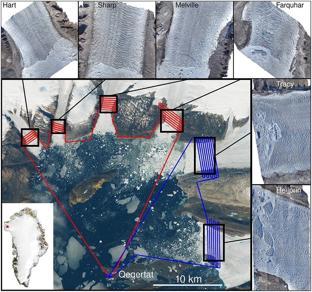
Figure 1. Sentinel-2A satellite image of the northeast most part of the Inglefield Bredning showing the settlement of Qeqertat and the six calving glaciers (Hart, Sharp, Melville, Farquhar, Tracy, and Heilprin) that we surveyed on 17 July 2017. The blue and red lines indicate the trajectory of the two daily UAV missions covering all glaciers. A map of Greenland (Source: MODIS) is displayed in the lower left and the location of the Inglefield Bredning is indicated by a red star.

The second field campaign was carried out at Eqip Sermia (69°48'N, 50°13'W) in the west sector of the GrIS (Figure 2) (Lüthi et al., 2016). The glacier discharges into the ocean through a 3.5 km wide calving front with ice flow of up to 15 m d⁻¹) near the terminus, and frequent calving activity (Walter et al., 2019). In July 2018, our base camp was located ~3 km south of Eqip Sermia's calving front (Figure 2).

FIGURE 2

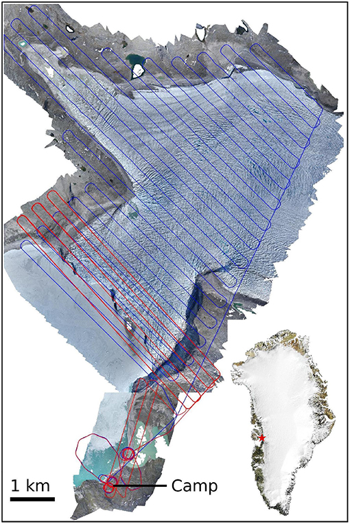
Figure 2. Ortho-image of Eqip Sermia acquired during a UAV survey on July 8. The lines show the trajectory of the UAV during the large-scale (blue) and repeat (red) missions, respectively. The ascending/descending spirals after take-off and before landing are denoted by the circular tracks around the camp. The area next to camp was also surveyed to assess the accuracy of photogrammetrical products in comparison with in situ GCPs. A map of Greenland (Source: MODIS) is displayed in the lower right and the location of Eqip Sermia glacier is indicated by a red star.

3. Unmanned Aerial Vehicle

3.1. Frame, Mechanical Components, and Batteries

Our fixed-wing UAV is based on the 2 m-wingspan “Skywalker X8” airframe (Figure 3), which is made from expanded polypropylene (EPP) foam. A powerful motor and large propeller (Table S1) were mounted at the back of the fuselage for rapid climb rates and for coping with the possibility of strong katabatic winds. The motor and electronics are powered by two 4S5P 16Ah Li-ion batteries (~1 kg each) providing a total of ~500 Wh. Li-ion batteries were preferred over Lithium-polymer batteries for two reasons: (1) they have a higher capacity to weight ratio, and (2) they maintain their capacity better in cold temperatures. In total, our UAV weighs ~4.75 kg including batteries and payload (i.e., camera), which is close to the recommended upper limit for this platform. During level flight in calm conditions, our UAV consumes ~100 W (after tuning parameters, section 3.2). All the components necessary to assemble the UAV are described in Supplementary S1 and cost ~$4,000 in total.

FIGURE 3

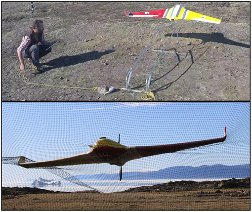
Figure 3. Take-off and landing in rough terrain: the fixed-wing UAV at take-off shortly after releasing the bungee (top), and during landing into the net (bottom).

3.2. Autopilot and Electronics

We equipped our UAV with the “Pixhawk” autopilot (Figure S1, https://pixhawk.org), which comes with GPS/compass, telemetry, air speed sensor, and battery management units. Additionally, we plugged a Remote Controller (RC) receiver to the Pixhawk so that the UAV can also be controlled manually by a pilot if necessary. Our autopilot runs under the open-source firmware arduplane 3.5.3 (http://ardupilot.org/ardupilot), which can be customized by changing parameters or more in-depth by modifying the code and recompiling the firmware. We tuned some flight parameters to make the platform more power-efficient (Supplementary S2 for details). We additionally de-activated the compass (and instead used the GPS) as we found it to be unreliable in the Inglefield Bredning (located at latitude 77°N) due to the proximity of the magnetic pole. Although we have not verified whether de-activating the compass at the latitude of Eqip Sermia glacier (located at latitude 70°N) was necessary, we kept this configuration for simplicity. The disadvantage of de-activating the compass is that one has to ensure a minimum ground speed to reliably estimate the heading from previous GPS positions. Therefore, we imposed a minimum ground speed of 5 m s⁻¹). This ensures that the UAV will maintain progress over ground even during strong head winds. All parameters that were changed from the default arduplane 3.5.3 configuration are given in Table S2.

3.3. On-Board Camera

The UAV was equipped with a Sony α6000 camera which features a 24 megapixel sensor (size: 23.5 × 15.6 mm; resolution: 6,000 × 4,000 pixel), equipped with a 16 mm Sony SEL16F29 lens. For all flights, our camera was preset to autofocus, ISO 400, and the aperture was chosen (depending on lighting conditions) to target a shutter speed of 1/2,000 s. For convenience, the camera was triggered directly by the Pixhawk autopilot such that trigger orders were included in the mission commands. This allowed us to use a distance-based camera trigger method which ensures that images are distributed uniformly over the target area with sufficient overlap.

3.4. Image Geo-Tagging Methods

In this study, the inaccessibility of the field sites prevented installation of GCPs next to the glaciers. To overcome this issue, the georeferencing of our photogrammetrical products relied directly on camera locations. These locations were estimated with different methods during each field campaign, as described in the two next paragraphs.

In July 2017 at Inglefield Bredning, camera locations were retrieved from the camera trigger events recorded in the log file of the autopilot. This initial method has several drawbacks: (i) the on-board GPS used for UAV navigation relies on standard positioning which has an absolute accuracy of up to 5 m horizontally and up to 30 m vertically, (ii) there is a delay between the time the camera is triggered and the time the image is effectively taken causing a discrepancy of up to several meters between the recorded trigger location and the true image location, (iii) the number of images collected after one flight is usually lower than the number of camera triggers recorded by the autopilot due to occasional missing images (~0.5% of images were missing in 2017). Drawbacks (i) and (ii) cause large geo-referencing errors while drawback (iii) requires a detection algorithm to match the images with the log files, which is not always reliable. We therefore opted for another, more accurate method during the 2018 field campaign.

In July 2018 at Eqip glacier, we followed Chudley et al. (2019) and used an extra differential carrier-phase GNSS receiver to record camera positions. We used two similar single-frequency Emlid Reach receivers (https://emlid.com/reach/), which are low-cost, light-weight, and log carrier-phase data: one fixed on the ground (called “base station”) to provide a stationary reference point and one (called “rover”) installed on the UAV and connected to the hot-shoe adaptor of our on-board camera. The two GNSS receivers were connected to a small antenna installed on 15 cm-long aluminum plates to filter reflected waves from below. Differential carrier-phase positioning yield ~1 centimeter accuracy (relative to the base station) as long as the distance between the two (base and rover) remain under 10 km, the differential ionospheric delay being negligible for such a small distance (Chudley et al., 2019). Although the Emlid receiver can be used for Real-Time Kinematic (RTK) (i.e., providing the accurate position of the UAV in real time), we used it only in post-processed kinematic mode for simplicity, i.e., we obtained the high accuracy by post-processing the log files of the rover and the base station after the completion of each flight. Lastly, we recorded the absolute position accuracy of the base station by the means of another differential but dual-frequency GPS Leica receiver.

3.5. Mission Planning and Ground Station

For each glacier, the UAVs trajectory was defined by a suite of waypoints describing parallel straight lines (Figures 1, 2) such that:

• the flight lines cover the glacier front uniformly and include 0.5–1 km of its bedrock margins for co-registration purposes (section 4.5) and accuracy assessment (section 5.2),

• the UAV maintains a constant elevation: ~800–850 m a.s.l. of between 450 and 800 m above glacier surface. This provides a ground sampling distance (GSD) of between ~0.15 and ~0.2 m (Table 1),

• the camera is triggered each time the UAV has moved 60 m horizontally, providing an image overlap of 95% in the flight direction. Although this is a high value, it ensures every part of the glacier surface is imaged, even during strong winds which may cause substantial pitch and roll,

• the lines are spaced such that the image overlap is at least 70% in cross-flight direction (Table 1),

• the lines are approximatively orthogonal to the ice flow direction (Figure 2).

TABLE 1

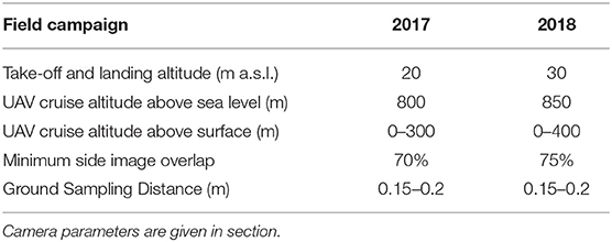
Table 1. Flight and photogrammetrical settings used at Ingelfield Bredning in 2017 and Eqip Sermia in 2018.

The command list was slightly different between the two field campaigns. In Inglefield Bredning (2017) the command list consisted of following commands:

1. Automatic take-off.

2. Fly to the first waypoint of the first glacier survey by climbing to the cruise altitude, i.e., 800 m a.s.l.

3. Perform the survey of the glacier.

4. Fly to the first waypoint of the next glacier survey following an obstacle-free trajectory and go back to step 3, otherwise go to step 5.

5. Fly back to the take-off and landing site by descending to 100 m above the ground.

6. Follow a predefined landing sequence.

At Eqip Sermia glacier each flight consisted of the following commands:

1. Automatic take-off.

2. Loiter and climb up to 850 m a.s.l., and fly to the first waypoint of the mapping sequence following an obstacle-free trajectory.

3. Perform the survey of Eqip Sermia glacier.

4. For repeat surveys, go to step 3 and loop three times.

5. Fly back to the take-off and landing site following an obstacle-free trajectory. Loiter and descent to 100 meters above the ground.

6. Follow a predefined landing sequence (Figure 2).

As a ground station, we used the free software “Mission Planner” (http://ardupilot.org/planner/) for two-way telemetry with the UAV autopilot. This includes the loading of mission commands, changing parameters, monitoring flight data, or ordering commands, such as the Return-To-Launch (RTL) command, which orders the UAV to immediately switch to Step 5. Prior to every flight, we used the Greenland Ice sheet Mapping Project (GIMP) DEM (Howat et al., 2014) to ensure that the UAV trajectory would not collide with the terrain during its mission. Once the command list was finalized, we uploaded it to the UAV using Mission Planner. To ensure uninterrupted telemetry connection, we operated the UAV from a clear view area, and used a 14 Dbi Yagi directional antenna which extended the range to over 30 km.

3.6. Take-Off With Bungee and Net Landing

Due to the additional weight of the UAV platform, caused by adding the large Li-Ion battery pack, we launched the UAV using a bungee catapult (Figure 3, top panel) described in Supplementary S3. This method was preferred to hand-launching which can be unreliable and dangerous (e.g., risk of cutting hand on the propeller). We also landed the UAV into a net (Figure 3, bottom panel), see Supplementary S4 for more details. This method was preferred to belly-landing which is difficult in polar regions due to the absence of smooth and flat terrain and would have risked damage and loss of aerodynamic efficiency.

4. Data Processing

4.1. Flight Data

We analyzed the performance of the UAV by interrogating the log files recorded by the Pixhawk autopilot to a 2 GB microSD card. In particular, we analyzed the power consumption, distance traveled, and wind strength.

4.2. Image Geo-Tagging

After each flight, we retrieved the horizontal and vertical coordinates of each image (i.e., geo-tagged the images) from the log files. This information was extracted from trigger orders recorded in the autopilot log files in 2017, and from the camera events recorded by the additional GNSS receiver in 2018. In the latter case, the log files of the two GNSS receivers (base and rover) were collected and processed by static differential carrier-phase positioning within the open-source software RTKLIB (http://www.rtklib.com/rtklib.htm). The centimeter-level accuracy of the camera locations recorded by the rover with respect to the base station position is obtained for the coordinate differences between base and rover in RTKLIB. The base station was positioned at a fixed location on bedrock for all flights and its absolute position was determined by the means of a dual-frequency Leica GPS receiver with the highest accuracy. This position is used to deduce accurate absolute positions of camera locations from the positions given by RTKLIB, whose the accuracy is relative to the base station.

4.3. SfM-MVS Photogrammetry

The images collected during all surveys were processed by structure-from-motion multi-view stereo (SfM-MVS) using the photogrammetrical software Agisoft PhotoScan (http://www.agisoft.com/). For each survey, PhotoScan performs the following steps:

• load images and camera locations,

• align images to build sparse point cloud (SfM step), using feature recognition and matching algorithms to obtain per-image depth maps, camera orientations, and calibrate the camera parameters,

• build dense point cloud (MVS step),

• export ortho-image at 0.25 m resolution and DEM at 0.5 m resolution.

In absence of GCPs, the geo-referencing was obtained directly by aerial triangulation from the camera locations (Chudley et al., 2019). More details on the SfM-MVS processing with Agisoft Photoscan, as well as data and parameters related to the processing of two UAV surveys are reported in Table S4.

4.4. Template Matching

Template matching is a well-established method for deriving glacier velocities from terrestrial (e.g., Ahn and Box, 2010; Messerli and Grinsted, 2015; Schwalbe and Maas, 2017), UAV (e.g., Ryan et al., 2015; Gindraux et al., 2017; Jouvet et al., 2017) or satellite (Sakakibara and Sugiyama, 2018) imageries. Here we used the Matlab toolbox ImGRAFT (http://imgraft.glaciology.net/) to derive high-resolution horizontal displacement fields, which was achieved by template matching (we used here normalized cross-correlation) of ortho-images (Messerli and Grinsted, 2015). For each glacier, template matching was applied over a pre-defined zone, which roughly covers the glacial area. Artifacts in the resulting displacement fields were filtered based on signal-to-noise ratio, velocity magnitude or direction, however this always represented <5% of the sampling. ImGRAFT parameters used for this study are reported in Table S5.

4.5. Co-registration

Prior to computing ice flow fields by template matching, pairs of ortho-images were co-registered to remove systematic errors and increase accuracy. For that purpose, template matching was first used to compute the shift of immobile off-glacier areas (example on Figure 10) between the two ortho-images. Thus, the mean shift was subtracted from the ice velocity field obtained by applying template matching a second time but over the glaciated area.

4.6. Maximum Principal Strain Rate

As in Jouvet et al. (2017), we computed the horizontal component of the strain rate tensor: D_ij = (∂_ju_i + ∂_iu_j)/2, where (u_x, u_y) is the horizontal velocity field inferred by template matching, and the derivatives are approximated by finite difference. Then, the maximum principal strain rate is the highest eigenvalue of D, which is the maximum normal strain rate among all possible directions.

4.7. DEM Differentiation

We used DEM differentiation to estimate the volume of ice (above the waterline only) that calved between two repeat flights. For each estimated calving event, we defined a mask covering the horizontal extent of the event from the corresponding ortho-images, and computed the DEM difference with MATLAB.

4.8. Uncertainty Assessment

Similarly to Chudley et al. (2019), the accuracy of the geo-referencing was assessed by measuring the shifts of two bedrock areas on each side of the glaciers between surveying products. For this purpose, we applied template matching (section 4.4) of ortho-images and DEM differentiation (section 4.7) to quantify the horizontal and the vertical deviations between surveys.

5. Results

In this section, we present the outcomes of UAV flights operated during the two field campaigns (Table 2) to demonstrate the potential of our UAV for glaciological studies in polar environments, and especially for large, inaccessible regions of rapid ice flow, such as tidewater glaciers.

TABLE 2

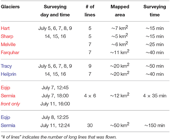
Table 2. Details of red and blue missions operated in 2017 in the Inglefield Bredning (Figure 1) and in 2018 at Eqip Sermia glacier (Figure 2).

In 2017, the red and blue missions of the six Inglefield Bredning glaciers were flown near-daily for 2 weeks whenever weather conditions allowed (Figure 1). In 2018, three repeat missions (red) focusing on the calving front and two large-scale missions (blue) of Eqip Sermia glacier were flown (Figure 2). Table 2, Table S3 give the list of all operated missions including key flight data, such as mapped areas, travel distances and flight durations.

5.1. UAV Performance

During the 2017 and 2018 field campaigns, our UAV was able to fly more than 20 missions longer than 150 km including two longer than 180 km (Table S3). The total duration of these flights was ~3 h. The analysis of power consumption (reported in Supplementary S8) demonstrated that flights of up to 200 km would have been possible while keeping a safety margin in terms of battery capacity, and that the battery capacity was not diminished significantly because of low temperatures during the flights (~0°C). The log data indicate that the UAV experienced wind up to 10 m/s with gusts up to 15 m/s, which is close to the cruising speed, during some of the 2017 blue mission flights (Table 2, Table S3). However, these conditions did not affect the UAV or the photogrammetrical results. Finally, despite the long distances (up to 30 km), the telemetry connection between the UAV and the operator was effective for 99% of the time during all missions.

5.2. Accuracy of Photogrammetrical Products

To compare successive surveys and extract information in terms of ice flow motion or iceberg calving, it is important that ortho-images and DEMs are accurately geo-referenced (or at least accurately co-registered). For the 2017 campaign in the Inglefield Bredning, we assessed their accuracies by computing the mean displacement of bedrock areas proximal Tracy and Hart glaciers of all the surveys (Table 2) relative to the first one (Figure 4). For the 2018 campaign at Eqip Sermia glacier, this was done between surveys of a same flight and between surveys of different flights (Figure 4).

FIGURE 4

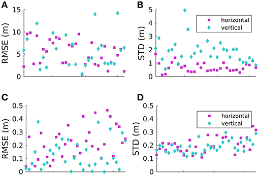
Figure 4. Horizontal and vertical RMSE (A,C) and STD (B,D) of the shifts of bedrock zones between repeat surveys inferred by template matching on ortho-images and DEM differentiation. Results of the field campaigns 2017 and 2018 are given separately. Note the different scales on the vertical axes.

In 2017, the root-mean-square error (RMSE) in the horizontal displacement field and the vertical RMSE from DEM differentiation were between 1 and 10 m, Figure 4A with a standard mean deviation (STD) of ~1 m horizontally and between 1 m and 3 m vertically (Figure 4B). By using an additional GNSS receiver to georeference the UAV images in 2018, the horizontal and vertical RMSE was reduced to <0.4 m (Figure 4C) with a STD <0.4 m (Figure 4D). The horizontal RMSE and STD even drop below 0.25 and 0.3 m when comparing surveys from a same flight (not shown). Our results highlight the strong gain of accuracy resulting from the geo-tagging method employed in 2018 as compared to 2017 which suffers from inaccurate camera locations recorded by the onboard GPS. Camera location error estimates reported by the SfM-MVS software Agisoft Photoscan show a reduction of the error by factor ~300 after adopting the 2018 method (Supplementary S6).

Our uncertainty assessment might include sub-pixel errors related to template matching, which potentially could be as large as 0.5 GSD (Chudley et al., 2019). Therefore, we additionally assessed the error using five GCPs installed next to the Eqip Sermia take-off and landing site in 2018 (Figure 2). In comparison to the GCP positions, which were surveyed using a differential dual-frequency Leica GPS, we found a horizontal discrepancy between 0.23 and 0.45 m in the DEMs produced using SfM-MVS photogrammetry. This corroborates with the template matching method used to uncertainty assessment presented above. However, we also found a vertical discrepancy between 0.65 and 1.21 m. As the unidirectional vertical shift (~0.6 m) is above the vertical RMSE found by DEM differentiation, we mostly attribute it to surveying inaccuracies, and to a lower extent to positioning discrepancies between the UAV camera and the on-board GNSS receiver (Chudley et al., 2019).

The estimated absolute uncertainty (0.4 m horizontally and vertically) in 2018 corresponds roughly to two times the ground sampling distances (GSDs). This is slightly less accurate than the accuracy reported in Chudley et al. (2019) with the similar equipment (same camera, optic, and GNSS receiver), although they used different SfM-MVS parameters and image compression formats. However, the STD values are approximatively twice as small. This shows that the relative accuracy between two ortho-images (and DEMs) can be reduced to ~1 GSD after co-registration, yielding to an accuracy similar to one reported in Chudley et al. (2019). It must be stressed that the horizontal and vertical STD are more than 10 and 5 times smaller, respectively, than the RMSE in 2017. This is a direct consequence of the improved image geo-tagging method used in 2018 compared to the one used in 2017 (section 3.4). Chudley et al. (2019) further analyzed the spatial pattern of the error and have shown that sloping areas are more subject to inaccuracies than flat areas.

5.3. Ortho-Images and DEMs

The large-scale surveys performed in 2017 and 2018 allowed us to produce high-resolution ortho-images and DEMs of seven glaciers and their marginal areas (Figures 1, 2). These reveal:

• that the front of Farquhar and Eqip Sermia glaciers are significantly sloping (not shown) and highly crevassed, while all other glaciers are fairly flat and less crevassed,

• the presence of water-filled crevasses on Sharp, Melville, Farquhar glaciers, and the presence of two supra-glacial lakes on Eqip Sermia glacier, including a major one between the glacier and its north-west margin,

• the presence of large tabular icebergs at the terminus of Melville, Farquhar, Tracy and Heilprin glaciers suggesting that their calving fronts are either floating or close to flotation (Bassis and Jacobs, 2013). This statement is supported by bathymetrical data (CReSIS, 2016; Sakakibara and Sugiyama, 2018), which demonstrate that the bedrock is ~300, 400, and 600 m below sea level at the calving fronts of Farquhar, Tracy, and Heilprin glaciers, and that ice is slightly thicker at the front.

5.4. Ice Flow Velocities

The accuracy of the ice surface displacement fields inferred by template matching depends on the time duration between the two surveys (the longer the time duration, the larger the displacement and the smaller the relative errors) and on the quality of the georeferencing. The latter was assessed in section 5.2 and was found to be ~20 times more accurate with the technique used in 2018 as compared to the one used in 2017. Figures 5–7 show 2 and 3 days separation surface ice flow velocities of four glaciers of the Inglefield Bredning in July 2017 and Eqip Sermia glacier in July 2018. Due to poor geo-referencing quality of the data of the Inglefield Bredning, the co-registration step was necessary to reduce the uncertainty to a reasonable value (from ~5 to ~1 m d⁻¹). In contrast, the ortho-images and DEMs derived from imagery collected at Eqip Sermia were accurately geo-referenced with an uncertainty of ~0.2 m d⁻¹ before co-registration, and ~0.1 m d⁻¹ after co-registration.

FIGURE 5

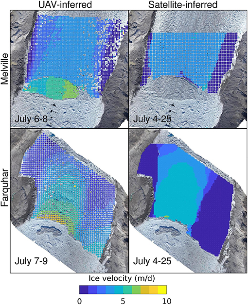
Figure 5. Horizontal ice speed inferred by UAV (2 days separation, left panels) and satellite images (21 days separation, right panels) in July 2017 at Melville (top panels) and Farquhar (bottom panels) glaciers. The velocity directions (not shown) are aligned with the fjord.

Our UAV-derived ice velocities compare closely with ice velocity fields obtained by template matching of 21 days separation Sentinel-2A pairs of ortho-images taken in July 2017 for four glaciers of the Inglefield Bredning (Figures 5, 6, right panels). Both UAV- and satellite-inferred velocity fields exhibit very similar magnitudes and spatial patterns: Melville, Farquhar, Tracy, and Heilprin glaciers exhibit UAV-inferred ice velocities of ~3.1, 4.3, 6.3, and 4 m d⁻¹ and satellite-inferred ice velocities of ~3.9, 4, 4.9, and 4.1 m d⁻¹ at the same location ~2 km upstream the calving front. The slight discrepancy between data is likely caused by aforementioned uncertainties in image georeferencing and template matching. In contrast, the higher discrepancy observed at Tracy glacier (Figure 6, top panels) could be due to ice flow variability since the UAV data covers 2 days while satellite data covers 21 days. The four glaciers exhibit fast ice flow at the front suggesting low basal resistance due to high buoyant forces (Vieli et al., 2000) in agreement with the observation of tabular icebergs (Bassis and Jacobs, 2013) and with ice thickness estimates and bathymetric data (Figure 5; Sakakibara and Sugiyama, 2018).

FIGURE 6

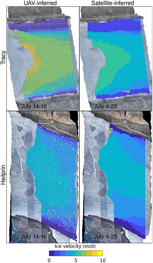
Figure 6. Horizontal ice speed inferred by UAV (2 days separation, left panels) and satellite images (21 days separation, right panels) in July 2017 at Tracy (top panels) and Heilprin (bottom panels) glaciers. The velocity directions (not shown) are aligned with the fjord.

Unlike ice flow at Melville, Tracy, and Heilprin glaciers, which is rather uniform along the central flowline and symmetrical along transversal profile (Figures 5, 6), the ice flow field of Farquhar glacier is more complex (Figure 5, bottom panels). While Farquhar has fast velocities near the terminus (up to 6–7 m d⁻¹), velocity diminishes rapidly upstream to ~4.5 m d⁻¹ ~2 km from the front. This strong velocity gradient can be explained by the bedrock topography, which is deep (~300 m) at the calving front but rises rapidly upstream (to ~100–150 m) with a relatively high surface slope (Figure 5; Sakakibara and Sugiyama, 2018). Gravitational effects rather than basal conditions are the main driver of the ice dynamics for this glacier. On the other hand, Farquhar glacier exhibits a dual regime at the front, namely fast flow in the western section and very slow motion in the eastern part within ~1 km from the glacier's margin (Figure 5, bottom panels). This pattern is similar to the one reported at Bowdoin glacier (Jouvet et al., 2017) and is expected to produce high horizontal shear and damage ice in agreement with the highly crevassed texture shown by the ortho-image (Figure 1). Following Jouvet et al. (2017), it is plausible that the slow ice flow region reflects a shallower bedrock in the eastern part, however, no information on the bedrock is currently available to verify or refute this hypothesis.

Eqip Sermia—for which we have the highest data coverage and accuracy—exhibits a complex and spatially highly variable ice flow pattern (Figure 7) different to the other glaciers: The ice moves at 1–2 m d⁻¹ in the eastern side along a 5-km wide transect toward the south-west and shrinks into a 3-km wide passage, where velocities reach ~10 m d⁻¹ near the front. In contrast, the lake-terminating part in the northern side is nearly stagnant. The surface structure of these two distinct parts clearly reflects the dynamics of ice: the fast part is highly crevassed and steep (as observed at Farquhar glacier) while the immobile part is nearly flat (Figure 2). The spatial pattern of the velocity field is similar to those derived from UAV surveys in August 2016 by Rohner et al. (2019) and Walter et al. (2019). It is likely that the velocity field presented here is representative of the flow of Eqip Sermia after 2014, when its terminus has accelerated up 10–15 m d⁻¹ (Lüthi et al., 2016).

FIGURE 7

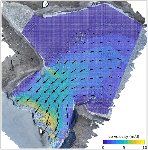
Figure 7. Three days separation horizontal ice flow velocity field of Eqip Sermia glacier obtained from the large-scale surveys performed on July 8 and 11.

5.5. Rifting of a Tabular Iceberg at Melville Glacier

The front of Melville glacier was captured by UAV on July 5, 6, 7, 8, and 9, and reveals the rifting and collapse (between July 8 and 9) of a major tabular iceberg 8. This iceberg has a surface area of ~0.3 km² and occupies more than two thirds of the calving front. According to Sentinel-2A satellite images (not shown), the crack first appeared between June 20 and 27, indicating that it had initiated, propagated, and collapsed within 12–19 days. The tip of the fracture appears in the same location on July 5, 6, and 7 but moved on July 8 by several hundreds of meters toward the west direction reaching nearly the glacier margin (see the red arrows on Figure 8).

FIGURE 8

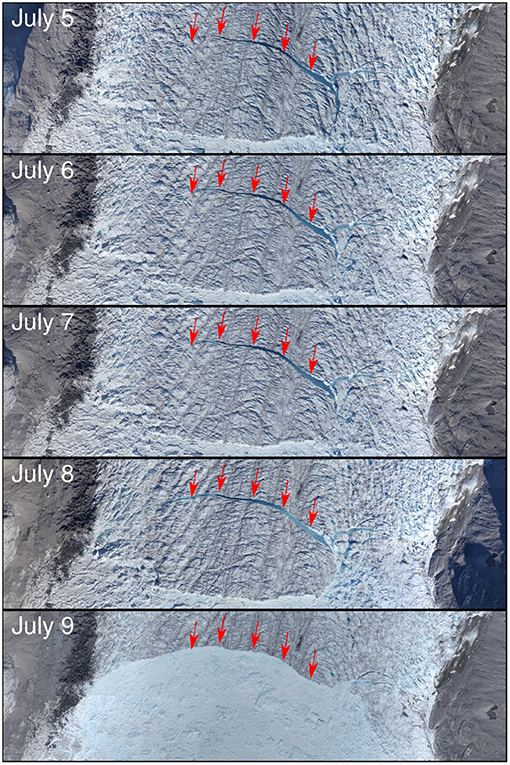
Figure 8. Ortho-images of the front of Melville glacier before (July 5, 6, 7, 8) and after (July 9) the separation of a major tabular iceberg. The red arrows show the path taken by the crack as observed on July 6 and 7. The substantial extension of the crack on July 8 suggests that it propagated step-wise before to collapse.

The propagation of the crack is even more apparent in the ice flow velocity fields, shown in Figure 9, which exhibit a clear discontinuity in the east-west direction. This discontinuity indicates high strain rates and demonstrates that an iceberg is detaching from the glacier on the eastern side, but remains attached to the other side. Interestingly, the gradient of velocity across the crack is relatively small between July 6 and 7 but becomes much larger 1 day later indicating a sharp acceleration of the crack opening within the 24 h preceding the final collapse (Figure 9). This acceleration demonstrates that the stress concentration at the crack tip must have increased and caused the crack to extend further laterally step-wise (Figure 9) before to collapse on July 7 or 8. As the width and length of the detached iceberg was larger than the thickness, it did not rotate and remained intact after detachment.

FIGURE 9

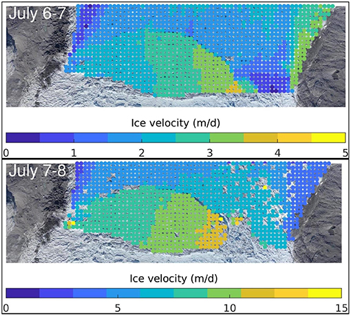
Figure 9. One day separation horizontal ice flow velocity fields of Melville glacier obtained from the three first ortho-images of Figure 8. Note that the range of the color bar varies.

This calving event shows similarities with the large event reported by Medrzycka et al. (2016) at Rink Isbræ, a 4.5 km wide calving glacier located in West Greenland. In their study, the authors argue that such large-scale, full-depth, mechanically driven calving events are promoted by deep bedrock and high ice velocities, suggesting that the calving front of Melville glacier might be close to floatation as well. Similar episodic extensions of a major crack responsible for the detachment of tabular icebergs have been reported for ice shelves by Bassis et al. (2005) and Joughin and MacAyeal (2005). Both studies point out that glaciological stresses lead to opening rates that accelerate with rift expansion, as observed here. The episodic propagation behavior can be explained by a reduced driving force due to the formation of a tip cavity after each propagation burst. Propagation events might have multiple and glacier-specific causes, including slumping of ice blocks into the rift (Bassis et al., 2005) or meltwater filling of the crack leading to hydro-fracturing (Van der Veen, 1998; Benn et al., 2007). Further field observations would be required to investigate the calving style observed at Melville glacier in July 2017.

5.6. Short-Term Ice Flow and Strain Rate Fields at Eqip Sermia

In addition to the 3 days average ice velocity field shown in Figure 7, we computed the ice flow motion at a higher temporal resolution from repeat surveys of the calving front. Since Eqip Sermia shows ice velocities up to 20 m d⁻¹ at the calving front, we expect a horizontal displacement of up to 1.5 m (or ~ 6–7 GSDs) within 105 min, which corresponds to the time period between the first and the last surveys of the repeat flights operated on July 7 (Table 2). As the displacement is only a few pixels, it was mandatory to co-register ortho-images (section 4.5) to achieve the highest accuracy. The uncertainty of the results scales with the RMSE of the displacement of the immobile zones (Figure 4), but is reduced to the STD after co-registration. For the ice flow inferred from the first and the last surveys of the first (resp. second) repeat missions, the correction step reduces the uncertainty from 2.8 m d⁻¹ (resp. 1.8 m d⁻¹) to 0.5 m d⁻¹ (resp. 0.7 m d⁻¹).

Figures 10a,b show two 105-min separation high-resolution (5 m) ice velocity fields inferred from the first and last surveys of the two July 7 repeat flights. Everywhere except in the immediate vicinity of the calving front, the two velocity fields agree fairly well and show smooth pattern of the ice dynamics as in Figure 7 or in a former UAV-inferred velocity field (Rohner et al., 2019; Walter et al., 2019). By contrast, the velocity field of the glacier front is spatially more erratic and varies greatly between the two flights (i.e., within 5 h). Comparatively, ice velocity fields inferred from terrestrial radar interferometry (Figure 3A in Walter et al., 2019) do not capture the roughness of the velocity field observed from UAV data presumably because of the low angle of observation. A plot of the corresponding maximum principal strain rates (section 4.6, Figure 10c) shows very localized extension across cracks revealing the uneven dynamic of the highly fragmented terminus of Eqip Sermia (Figure 2).

FIGURE 10

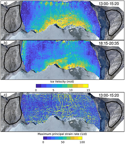
Figure 10. High-resolution (5 m) horizontal ice flow velocity (a,b) and maximum strain rate (c) over 105 min at the front of Eqip Sermia inferred from the ortho-images of repeat survey missions performed on 7 July 2018. Polygons on the glacier sides indicate off-glacier areas used for co-registration.

This highlights the capacity of our high-endurance UAV to capture the ice flow in high spatial resolution and at short time scales relevant for the fracturing of ice or for tidally driven processes. Our shortest duration ice flow velocity field is more than three times shorter than the shortest one reported by Chudley et al. (2019) for a twice faster calving glacier using similar UAV-based techniques.

5.7. Calving Volumes at Eqip Sermia

Eqip Sermia is known to exhibit intense calving activity (Lüthi and Vieli, 2016), i.e., small icebergs calve frequently. The volume of iceberg discharge can be estimated by differencing DEMs of the calving front before and after calving events (Walter et al., 2019). One difficulty of this approach is that both processes—ice flow and iceberg calving—constantly reshape the front geometry. The only strategy to isolate the two is to difference DEMs with a short revisit period so that the dynamics of the glacier cause negligible changes during this period. However, this strategy is conditioned to the availability of frequent DEMs, which is made possible thanks to the high endurance of our UAV. Figure 11 shows two examples of DEM differentiation applied to two calving events of different size.

FIGURE 11

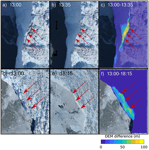
Figure 11. For each row, the first and second panel shows ortho-images before and after a calving event occurred at Eqip Sermia on 7 July 2018, while the third panel shows the difference of the two corresponding DEMs. (a–c) refer to a small-scale event that occurred between 13:00 and 13:35, while (d–f) refer to a larger event that occurred between 13:00 and 18:15.

In Figures 11a–c, a small-scale calving event occurred between the first and the second surveys in an area moving at ~15 m d⁻¹ (Figure 10). Therefore, the difference between the two corresponding DEMs gives the best estimation of the ice volume lost by calving, i.e., ~3.3 × 10⁴ m³—the ice displacement of this zone being of only ~0.3 m between the two surveys. To evaluate the impact of this displacement as a possible source of error in the estimation, we also differentiated DEMs from the third and forth surveys with respect to the first one. The results shown in Figure 12 indicate that the ice displacement has a significant impact, e.g., the pair first-third changes the volume estimation by more than 30%. Compared to the first-second pair, this discrepancy is reduced to 20% by differentiating DEMs that were corrected for the ice flow field. Our results therefore emphasize that highly frequent DEMs of the glacier front are necessary to accurately capture small-scale calving events in the order of 10⁴ m³ as less frequent DEMs—even corrected to account for ice motion—still yield large uncertainties. Using terrestrial SfM-MVS, Mallalieu et al. (2017) already pointed out the need for frequent DEMs for this purpose.

FIGURE 12

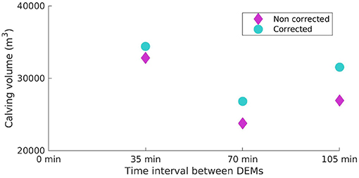
Figure 12. Volume of ice lost by calving obtained by differentiating the DEMs of the second, third, and forth surveys with respect to the first one for the calving event shown on Figures 11a–c. The method was first applied to raw DEMs, and second to DEMs horizontally shifted to compensate the ice displacement.

As the relative uncertainty of calving volumes induced by inter-survey ice displacement scales with the calving size, the estimation a larger scale calving volumes (Figures 11d–f) is less affected by this source of error. The 16 possible DEM differentiations between the four surveys of both flights—which were operated with more than 5 h of time separation in a similarly fast-moving zone—indicates a mean ice volume of 9.1 × 10⁵ m³ with a standard deviation of 3.8 × 10⁴ m³, i.e., 4% of the mean ice volume. In this case, the calving event is thus sufficiently big such that the ice motion over 5–7 h has negligible effects on the volume computation. Unlike the first small-scale calving event, the second one has a submarine component (Compare Figures 11d,e), which cannot be evaluated from aerial images. This volume estimate must therefore be considered as a lower bound.

Our results shed light on the potential of repeat UAV SfM-MVS to accurately capture the morphology of calving fronts before and after the occurrence of calving events, and reliably estimate their volumes. By contrast, terrestrial SfM-MVS (Mallalieu et al., 2017) permits continuous monitoring but suffers from high uncertainty with shape reconstruction and volume estimation. This emphasizes the complementary nature of aerial and terrestrial approaches to reliably quantify the volume and frequency of calving events over long time periods (e.g., Minowa et al., 2019).

6. Conclusions

We have presented a low-cost high-endurance fixed-wing UAV designed for large-scale and/or repeat photogrammetrical surveys of glaciers in polar regions. Our custom-built UAV allowed us to perform 48 glacier surveys across Inglefield Bredning in July 2017 and 14 surveys of Eqip Sermia glacier in July 2018, including multiple glaciers, single large-scale, and multiple smaller-scale surveys. The primary achievements include:

• Autonomous UAV surveys over long distances (up to 180 km) and during long duration (up to ~3 h) for mapping up to four calving glacier termini located more than 25 km away from the UAV operator or ~50 km² of a single glacier, which is several times larger than in any other glacier area mapped by UAV in former studies (Ryan et al., 2015; Jouvet et al., 2017; Chudley et al., 2019).

• Overcoming adverse conditions often associated with polar environments, such as (i) the roughness of the terrain for take-off and landing in confined areas; (ii) the occurrence of katabatic winds of up to 15 m/s; (iii) the steep inclination angle of the magnetic field in high latitudes, which causes a weak horizontal vector for measuring magnetic North with a compass; (iv) cold temperatures (~ 0°C), which might reduce the battery capacity.

• Production of large-scale (~50 km²), high-resolution (0.25–0.5 m), and accurately geo-referenced (1–2 pixels) ortho-images, DEMs, and ice flow displacement fields using SfM-MVS photogrammetry and template matching and without using any GCPs.

• Generation of 105-min separation ice flow velocity fields of the front of Eqip Sermia revealing the uneven and fluctuating dynamic of its most fragmented area at the scale of individual crack. This data may be especially useful for understanding fracturing processes of ice responsible for calving. To our knowledge this is the shortest time period of glacial motion captured by UAV photogrammetry.

• Tracking the propagation of rifts during the detachment of tabular icebergs. Such data in high temporal resolution during the final phase shortly before the collapse are key for understanding the processes leading to this type of calving event, and could not be collected by satellite remote sensing.

• Collection of frequent DEMs to accurately calculate the volume of ice lost during small-scale calving events as the computation can be biased by ice motion if the return period is too long. To our knowledge, this is the first time that UAV photogrammetry was used to generate sub-hour separation repeat DEMs.

Two features of our UAV were essential for capturing short-term glacial processes, such as ice flow, fracture and the release of icebergs at unprecedented resolution and accuracy. First, its high endurance was crucial not only to cover large glacial areas, but also to perform repeat surveys that could track these processes within a few hours. Second, GNSS-based aerial triangulation was key to accurately geo-reference the results without using any GCPs, and to make it possible to precisely compare successive surveys.

The approach presented in this study has potential to quantify iceberg calving of all sizes and/or measure the short-term variability of surface flow fields in complementary manner to existing observational methods, such as terrestrial time-lapse photogrammetry (e.g., Rosenau et al., 2013; James et al., 2014; Murray et al., 2015), radar interferometry (e.g., Walter et al., 2019), in-situ GPS and seismic measurements (e.g., Bassis and Jacobs, 2013), or remote sensing (e.g., Joughin and MacAyeal, 2005; Rohner et al., 2019). It would have been possible to infer sub-hour ice flow velocity fields at Eqip Sermia by flying twice as low to the surface (or equivalently halving the GSD). Our UAV may therefore be of interest for investigating:

• tidal driven variability of the ice flow of ocean-terminating glaciers (Sugiyama et al., 2015) or the tidal flexure of ice shelves, which be can used to locate the grounding line (Le Meur et al., 2014),

• short-lived speed-up events caused by a abrupt change in the subglacial hydrological system (e.g., Jouvet et al., 2018),

• fracturing processes, such as small-scale calving (Walter et al., 2019) or the rifting of a tabular icebergs (Joughin and MacAyeal, 2005; Bassis and Jacobs, 2013; Medrzycka et al., 2016).

7. Perspectives

Our study demonstrates the potential of high-endurance UAVs to monitor glacial processes at high spatial and temporal resolution. Although our UAV can fly long distances compared to the majority of battery-powered fixed-wing UAVs in this category (<5 kg), there exist other platforms that can fly much longer offering promising perspectives for the monitoring of remote glaciers in terms of coverage and revisit frequency. There exist several alternatives to increase the range of fixed-wing UAVs. First, UAV performance can be improved by increasing the wingspan, however, this usually makes the structure more fragile and the UAV less robust to katabatic winds. Second, using a gas-powered engine can extend the range by several factors compared to battery-power, however, at the prize of adding system complexity and increasing the risks of mechanical failure. Lastly, solar-electrically powered fixed-wing UAV promise significantly increased flight endurance over purely-electrically or even gas-powered aerial vehicles. A solar-powered UAV uses excess solar energy gathered during the day to recharge its batteries. Given an appropriate design and suitable environmental conditions, the stored energy may even be sufficient to continuously keep the UAV airborne during the night and, potentially, subsequent days. For instance, the 6.9 kg AtlantikSolar UAV (Oettershagen et al., 2016) made a continuous and solely solar-powered flight of 81.5 h and more than 2,000 km ground distance in the summer of 2015. Although experimental, solar-powered UAVs are great candidates for continuous glacier monitoring in remote areas.

High-endurance UAVs have potential as remote sensing platforms beyond glaciology, e.g., to perform meteorological measurements or observations of fauna whenever satellite imagery are not sufficiently resolved or frequent to fulfill this task. Manned aircraft can partly cover the need for high space resolution data, but the costs for repeat operations become prohibitively expensive. In this context, the primary advantages of using UAVs, compared to manned airplanes, for such missions are the low costs, the ease of repeating surveys, and mitigation of pilot's safety issues. Therefore, the increasing endurance of UAVs as well as the miniaturization of payloads indicates that the capability of scanning very remote areas will keep augmenting. This technology may therefore complement satellite remote sensing, especially in polar regions, as well as ground-based instruments, such as terrestrial time-lapse photogrammetry, terrestrial radar interferometry, or in-situ GPS and seismic measurements for monitoring the dynamical processes of glaciers.

Data Availability

The datasets (orthoimages and digital elevation models) generated for this study can be found in the following repositories:

• http://doi.org/10.5281/zenodo.3340177 (Hart, Sharp, Melville, and Farquhar glaciers).

• http://doi.org/10.5281/zenodo.3338646 (Heilprin glacier).

• http://doi.org/10.5281/zenodo.3337803 (Tracy glacier).

• http://doi.org/10.5281/zenodo.3337242 (Eqip glacier).

Raw data are available upon request.

Author Contributions

GJ designed the study and wrote the paper with support from all co-authors. GJ and YW developed the UAV with the assistance of JR. GJ and EvD processed the aerial images by SfM-MVS. The UAV was operated by GJ and YW in the Inglefield Bredning (2017) and by GJ and EvD at Eqip Sermia (2018). ML and AV organized the fieldwork at Eqip Sermia in July 2018.

Funding

The field work in the Inglefield Bredning was supported by the Dr. Alfred and Flora Spätli Fund and the ETH Foundation Grant ETH-12 16-2 (Sun2Ice Project). The field work at Eqip Sermia was funded by Swiss National Science Foundation grant SNF 200021 156098 and the Swiss Polar Institute (2018 Polar Access Fund of EvD).

Conflict of Interest Statement

The authors declare that the research was conducted in the absence of any commercial or financial relationships that could be construed as a potential conflict of interest.

Acknowledgments

The authors wish to acknowledge Martin Funk for his strong support and his helpful comments on the manuscript, Andreas Bauder for processing the positions measured by the dual-frequency Leica GPS receiver, Julien Seguinot for providing Sentinel-2A satellite images (processed with SentinelFlow), Daiki Sakakibara for providing yearly-average velocities of Tracy and Heilprin glaciers for comparison, and Tom Chudley for sharing experience with the Emlid Reach GNSS receiver. We thank Thomas Wyder, Daniel Gubser, Rolf Jäger, Oliver Fontana for their support to construct and fly the X8 UAV, respectively. Fabian Neyer was acknowledged for his support to process the UAV data by SfM-MVS.

Supplementary Material

The Supplementary Material for this article can be found online at: https://www.frontiersin.org/articles/10.3389/feart.2019.00206/full#supplementary-material

References

Ahn, Y., and Box, J. E. (2010). Glacier velocities from time-lapse photos: technique development and first results from the extreme ice survey (EIS) in greenland. J. Glaciol. 56, 723–734. doi: 10.3189/002214310793146313

CrossRef Full Text | Google Scholar

Bash, E., Moorman, B., and Gunther, A. (2018). Detecting short-term surface melt on an arctic glacier using uav surveys. Rem. Sens. 10:1547. doi: 10.3390/rs10101547

CrossRef Full Text | Google Scholar

Bassis, J., and Jacobs, S. (2013). Diverse calving patterns linked to glacier geometry. Nat. Geosci. 6:833. doi: 10.1038/ngeo1887

CrossRef Full Text | Google Scholar

Bassis, J. N., Coleman, R., Fricker, H., and Minster, J. (2005). Episodic propagation of a rift on the amery ice shelf, East Antarctica. Geophys. Res. Lett. 32:L06502. doi: 10.1029/2004GL022048

CrossRef Full Text | Google Scholar

Benn, D. I., Warren, C. R., and Mottram, R. H. (2007). Calving processes and the dynamics of calving glaciers. Earth Sci. Rev. 82, 143–179. doi: 10.1016/j.earscirev.2007.02.002

CrossRef Full Text | Google Scholar

Bhardwaj, A., Sam, L., Martín-Torres, F. J., Kumar, R., et al. (2016). UAVs as remote sensing platform in glaciology: present applications and future prospects. Rem. Sens. Environ. 175, 196–204. doi: 10.1016/j.rse.2015.12.029

CrossRef Full Text | Google Scholar

Cassano, J. J., Seefeldt, M. W., Knuth, S. L., Bradley, A. C., Herrman, P. D., Kernebone, P. A., et al. (2016). Observations of the atmosphere and surface state over terra nova bay, antarctica, using unmanned aerial systems. Earth Syst. Sci. Data 8:115. doi: 10.5194/essd-8-115-2016

CrossRef Full Text | Google Scholar

Chudley, T. R., Christoffersen, P., Doyle, S. H., Abellan, A., and Snooke, N. (2019). High-accuracy uav photogrammetry of ice sheet dynamics with no ground control. Cryosphere 13, 955–968. doi: 10.5194/tc-13-955-2019

CrossRef Full Text | Google Scholar

CReSIS (2016). Center for Remote Sensing of Ice Sheets (CReSIS) Level 2 Radar Data. Lawrence, KS: Digital Media.

Crocker, R. I., Maslanik, J. A., Adler, J. J., Palo, S. E., Herzfeld, U. C., and Emery, W. J. (2012). A sensor package for ice surface observations using small unmanned aircraft systems. IEEE Trans. Geosci. Rem. Sens. 50, 1033–1047. doi: 10.1109/TGRS.2011.2167339

CrossRef Full Text | Google Scholar

Ely, J. C., Graham, C., Barr, I. D., Rea, B. R., Spagnolo, M., and Evans, J. (2017). Using uav acquired photography and structure from motion techniques for studying glacier landforms: application to the glacial flutes at isfallsglaciären. Earth Surf. Process. Landforms 42, 877–888. doi: 10.1002/esp.4044

CrossRef Full Text | Google Scholar

Fraser, R. H., Olthof, I., Lantz, T. C., and Schmitt, C. (2016). UAV photogrammetry for mapping vegetation in the low-arctic. Arctic Sci. 2, 79–102. doi: 10.1139/as-2016-0008

CrossRef Full Text | Google Scholar

Gindraux, S., Boesch, R., and Farinotti, D. (2017). Accuracy assessment of digital surface models from unmanned aerial vehicles' imagery on glaciers. Rem. Sens. 9:186. doi: 10.3390/rs9020186

CrossRef Full Text | Google Scholar

Higashino, S., and Funaki, M. (2013). Development and flights of ant-plane uavs for aerial filming and geomagnetic survey in Antarctica. J. Unmanned Syst. Technol. 1, 37–42. doi: 10.21535%2Fjust.v1i2.19

CrossRef Full Text | Google Scholar

Hodson, A., Anesio, A. M., Ng, F., Watson, R., Quirk, J., Irvine-Fynn, T., et al. (2007). A glacier respires: quantifying the distribution and respiration CO₂ flux of cryoconite across an entire arctic supraglacial ecosystem. J. Geophys. Res. Biogeosci. 112:G04S36. doi: 10.1029/2007JG000452

CrossRef Full Text | Google Scholar

Howat, I., Negrete, A., and Smith, B. (2014). The Greenland ice mapping project (gimp) land classification and surface elevation data sets. Cryosphere 8, 1509–1518. doi: 10.5194/tc-8-1509-2014

CrossRef Full Text | Google Scholar

Immerzeel, W., Kraaijenbrink, P., Shea, J., Shrestha, A., Pellicciotti, F., Bierkens, M., et al. (2014). High-resolution monitoring of himalayan glacier dynamics using unmanned aerial vehicles. Rem. Sens. Environ. 150, 93–103. doi: 10.1016/j.rse.2014.04.025

CrossRef Full Text | Google Scholar

James, T. D., Murray, T., Selmes, N., Scharrer, K., and O'Leary, M. (2014). Buoyant flexure and basal crevassing in dynamic mass loss at helheim glacier. Nat. Geosci. 7:593. doi: 10.1038/ngeo2204

CrossRef Full Text | Google Scholar

Jones, C., Ryan, J., Holt, T., and Hubbard, A. (2018). Structural glaciology of isunguata sermia, West Greenland. J. Maps 14, 517–527. doi: 10.1080/17445647.2018.1507952

CrossRef Full Text | Google Scholar

Joughin, I., and MacAyeal, D. R. (2005). Calving of large tabular icebergs from ice shelf rift systems. Geophys. Res. Lett. 32. doi: 10.1029/2004GL020978

CrossRef Full Text | Google Scholar

Jouvet, G., van Dongen, E., Lüthi, M. P., and Vieli, A. (2019). In-situ measurements of the ice flow motion at Eqip Sermia glacier using a remotely controlled UAV. Geosci. Instr. Methods Data Syst. Discuss. 2019, 1–15. doi: 10.5194/gi-2019-6

CrossRef Full Text | Google Scholar

Jouvet, G., Weidmann, Y., Kneib, M., Detert, M., Seguinot, J., Sakakibara, D., et al. (2018). Short-lived ice speed-up and plume water flow captured by a vtol uav give insights into subglacial hydrological system of Bowdoin glacier. Rem. Sens. Environ. 217, 389–399. doi: 10.1016/j.rse.2018.08.027

CrossRef Full Text | Google Scholar

Jouvet, G., Weidmann, Y., Seguinot, J., Funk, M., Abe, T., Sakakibara, D., et al. (2017). Initiation of a major calving event on the bowdoin glacier captured by UAV photogrammetry. Cryosphere 11, 911–921. doi: 10.5194/tc-11-911-2017

CrossRef Full Text | Google Scholar

Le Meur, E., Sacchettini, M., Garambois, S., Berthier, E., Drouet, A., Durand, G., et al. (2014). Two independent methods for mapping the grounding line of an outlet glacier–an example from the Astrolabe glacier, Terre adélie, Antarctica. Cryosphere 8, 1331–1346. doi: 10.5194/tc-8-1331-2014

CrossRef Full Text | Google Scholar

Lüthi, M. P., and Vieli, A. (2016). Multi-method observation and analysis of a tsunami caused by glacier calving. Cryosphere 10, 995–1002. doi: 10.5194/tc-10-995-2016

CrossRef Full Text | Google Scholar

Lüthi, M. P., Vieli, A., Moreau, L., Joughin, I., Reisser, M., Small, D., et al. (2016). A century of geometry and velocity evolution at Eqip Sermia, west greenland. J. Glaciol. 62, 640–654. doi: 10.1017/jog.2016.38

CrossRef Full Text | Google Scholar

Mallalieu, J., Carrivick, J. L., Quincey, D. J., Smith, M. W., and James, W. H. (2017). An integrated structure-from-motion and time-lapse technique for quantifying ice-margin dynamics. J. Glaciol. 63, 937–949. doi: 10.1017/jog.2017.48

CrossRef Full Text | Google Scholar

Medrzycka, D., Benn, D. I., Box, J. E., Copland, L., and Balog, J. (2016). Calving behavior at rink isbræ, west greenland, from time-lapse photos. Arctic Antarctic Alpine Res. 48, 263–277. doi: 10.1657/AAAR0015-059

CrossRef Full Text | Google Scholar

Messerli, A., and Grinsted, A. (2015). Image georectification and feature tracking toolbox: Imgraft. Geosci. Instr. Methods Data Syst. 4, 23–34. doi: 10.5194/gi-4-23-2015

CrossRef Full Text | Google Scholar

Minowa, M., Podolskiy, E. A., Jouvet, G., Weidmann, Y., Sakakibara, D., Tsutaki, S., et al. (2019). Calving flux estimation from tsunami waves. Earth Planet. Sci. Lett. 515, 283–290. doi: 10.1016/j.epsl.2019.03.023

CrossRef Full Text | Google Scholar

Moreland, E., Cameron, M., Angliss, P. R., and Boveng, L. P. (2015). Evaluation of a ship-based unoccupied aircraft system (UAS) for surveys of spotted and ribbon seals in the Bering sea pack ice. J. Unmanned Veh. Syst. 3, 114–122. doi: 10.1139/juvs-2015-0012

CrossRef Full Text | Google Scholar

Murray, T., Selmes, N., James, T. D., Edwards, S., Martin, I., O'Farrell, T., et al. (2015). Dynamics of glacier calving at the ungrounded margin of Helheim glacier, Southeast Greenland. J. Geophys. Res. Earth Surf. 120, 964–982. doi: 10.1002/2015JF003531

PubMed Abstract | CrossRef Full Text | Google Scholar

Oettershagen, P., Melzer, A., Mantel, T., Rudin, K., Stastny, T., Wawrzacz, B., et al. (2016). “Perpetual flight with a small solar-powered UAV: flight results, performance analysis and model validation,” in Proceedings of the 2016 IEEE Aerospace Conference (AERO 2016) (Big Sky, MT: IEEE), 7500855.

Google Scholar

Pavelka, K., Faltỳnová, M., Hlaváčová, I., Šedina, J., and Matoušková, E. (2016). Using remote sensing and rpas for archeology and monitoring in Western Greenland. Int. Arch. Photogrammetry Rem. Sens. Spatial Inform. Sci. 41, 979–983. doi: 10.5194/isprsarchives-XLI-B1-979-2016

CrossRef Full Text

Podgorny, I., Lubin, D., and Perovich, D. K. (2018). Monte Carlo study of UAV-measurable Albedo over Arctic sea ice. J. Atmos. Ocean. Technol. 35, 57–66. doi: 10.1175/JTECH-D-17-0066.1

CrossRef Full Text | Google Scholar

Rignot, E., and Kanagaratnam, P. (2006). Changes in the velocity structure of the greenland ice sheet. Science 311, 986–990. doi: 10.1126/science.1121381

PubMed Abstract | CrossRef Full Text | Google Scholar

Rippin, D. M., Pomfret, A., and King, N. (2015). High resolution mapping of supra-glacial drainage pathways reveals link between micro-channel drainage density, surface roughness and surface reflectance. Earth Surf. Process. Landforms 40, 1279–1290. doi: 10.1002/esp.3719

CrossRef Full Text | Google Scholar

Rohner, C., Small, D., Henke, D., Lüthi, M. P., and Vieli, A. (2019). Multisensor validation of tidewater glacier flow fields derived from sar intensity tracking. Cryosphere Discuss. 2019, 1–27. doi: 10.5194/tc-2018-278

CrossRef Full Text

Rosenau, R., Schwalbe, E., Maas, H.-G., Baessler, M., and Dietrich, R. (2013). Grounding line migration and high-resolution calving dynamics of Jakobshavn Isbræ, West Greenland. J. Geophys. Res. Earth Surf. 118, 382–395. doi: 10.1029/2012JF002515

CrossRef Full Text | Google Scholar

Ryan, J. C., Hubbard, A., Box, J. E., Brough, S., Cameron, K., Cook, J. M., et al. (2017). Derivation of high spatial resolution albedo from UAV digital imagery: application over the greenland ice sheet. Front. Earth Sci. 5:40. doi: 10.3389/feart.2017.00040

CrossRef Full Text | Google Scholar

Ryan, J. C., Hubbard, A., Stibal, M., Irvine-Fynn, T. D., Cook, J., Smith, L. C., et al. (2018). Dark zone of the greenland ice sheet controlled by distributed biologically-active impurities. Nat. Commun. 9:1065. doi: 10.1038/s41467-018-03353-2

PubMed Abstract | CrossRef Full Text | Google Scholar

Ryan, J. C., Hubbard, A. L., Box, J. E., Todd, J., Christoffersen, P., Carr, J. R., et al. (2015). UAV photogrammetry and structure from motion to assess calving dynamics at store glacier, a large outlet draining the greenland ice sheet. Cryosphere 9, 1–11. doi: 10.5194/tc-9-1-2015

CrossRef Full Text | Google Scholar

Sakakibara, D., and Sugiyama, S. (2018). Ice front and flow speed variations of marine-terminating outlet glaciers along the coast of Prudhoe land, Northwestern Greenland. J. Glaciol. 64, 300–310. doi: 10.1017/jog.2018.20

CrossRef Full Text | Google Scholar

Schwalbe, E., and Maas, H.-G. (2017). The determination of high-resolution spatio-temporal glacier motion fields from time-lapse sequences. Earth Surf. Dyn. 5:861. doi: 10.5194/esurf-5-861-2017

CrossRef Full Text | Google Scholar

Stibal, M., Box, J. E., Cameron, K. A., Langen, P. L., Yallop, M. L., Mottram, R. H., et al. (2017). Algae drive enhanced darkening of bare ice on the Greenland ice sheet. Geophys. Res. Lett. 44, 463–471. doi: 10.1002/2017GL075958

CrossRef Full Text | Google Scholar

Sugiyama, S., Sakakibara, D., Tsutaki, S., Maruyama, M., and Sawagaki, T. (2015). Glacier dynamics near the calving front of Bowdoin glacier, Northwestern Greenland. J. Glaciol. 61, 223–232. doi: 10.3189/2015JoG14J127

CrossRef Full Text | Google Scholar

Tonkin, T. N., Midgley, N., Cook, S. J., and Graham, D. J. (2016). Ice-cored moraine degradation mapped and quantified using an unmanned aerial vehicle: a case study from a polythermal glacier in Svalbard. Geomorphology 258, 1–10. doi: 10.1016/j.geomorph.2015.12.019

CrossRef Full Text | Google Scholar

Van der Veen, C. (1998). Fracture mechanics approach to penetration of surface crevasses on glaciers. Cold Regions Sci. Technol. 27, 31–47. doi: 10.1016/S0165-232X(97)00022-0

CrossRef Full Text | Google Scholar

Vieli, A., Funk, M., and Blatter, H. (2000). Tidewater glaciers: frontal flow acceleration and basal sliding. Ann. Glaciol. 31, 217–221. doi: 10.3189/172756400781820417

CrossRef Full Text | Google Scholar

Walter, A., Lüthi, M. P., and Vieli, A. (2019). Calving event size measurements and statistics of Eqip Sermia, Greenland, from terrestrial radar interferometry. Cryosphere Discuss. 2019, 1–23. doi: 10.5194/tc-2019-102

CrossRef Full Text | Google Scholar

Westoby, M. J., Dunning, S. A., Woodward, J., Hein, A. S., Marrero, S. M., Winter, K., et al. (2015). Sedimentological characterization of antarctic moraines using UAVs and structure-from-motion photogrammetry. J. Glaciol. 61, 1088–1102. doi: 10.3189/2015JoG15J086

CrossRef Full Text | Google Scholar

Willis, J. K., Carroll, D., Fenty, I., Kohli, G., Khazendar, A., Rutherford, M., et al. (2018). Ocean-ice interactions in inglefield gulf: early results from nasa's oceans melting Greenland mission. Oceanography 31, 100–108. doi: 10.5670/oceanog.2018.211

CrossRef Full Text | Google Scholar

Zmarz, A., Korczak-Abshire, M., Storvold, R., Rodzewicz, M., and Kedzierska, I. (2015). Indicator species population monitoring in antarctica with UAV. Int. Arch. Photogrammetry Rem. Sens. Spatial Inform. Sci. 40:189. doi: 10.5194/isprsarchives-XL-1-W4-189-2015

CrossRef Full Text | Google Scholar