Ensemble-Averaging Resolves Rapid Atmospheric Response to the 2017 Total Solar Eclipse

Rapid changes in solar radiative forcing influence heat, scalar and momentum fluxes and thereby shift the trajectory of near-surface atmospheric transitions. Surface fluxes are difficult to obtain during atmospheric transitions by either bulk or eddy-covariance methods because both techniques assume quasi-stationarity in an atmospheric state and require sufficiently long blocks of data, typically on the order of 10–30 min, to obtain statistically significant results. These computational requirements limit the temporal resolution of atmospheric processes that researchers can examine using traditional measurement techniques. In this paper, we present a novel observational approach to calculate surface fluxes at sub-minute temporal resolutions. High-frequency data from a horizontal, log-spaced array of nine time-synchronized ultrasonic anemometers were used to perform spatial-temporal ensemble averaging and to obtain eddy-covariance turbulence fluxes at unprecedented time resolutions. The 2017 Great American Solar Eclipse event provided a “natural experiment” to test the ensemble-observation and averaging approach. A total eclipse is energetically well-constrained and, unlike day/night transitions, is a perturbation that quickly transitions from and back to a state of significant solar forcing, providing an ideal scenario for testing the space-timescales required for surface flux calculations. Additionally, two Doppler lidars and a vertically-oriented Distributed Temperature Sensing (DTS) system provided measurements to characterize near-surface atmospheric conditions. Results show that the ensemble-averaged sensible heat fluxes converged at timescales as short as 15 s. Additional analyses show that the timescale of the connection between the surface and the atmosphere is more rapid than previous measurements have been capable of showing and is on the order of 10 min or less. This experiment demonstrates that ensemble-flux measurements are capable of resolving fluctuations in surface fluxes during rapid atmospheric transitions.

Introduction

Solar eclipses are a natural experiment (Harrison and Hanna, 2016) for which the land and atmosphere responses to changes in insolation, which are more rapid than during the morning and evening transitions, can be investigated (Antonia et al., 1979; Eaton et al., 1997; Foken et al., 2001). Past studies have shown that a solar eclipse is associated with a number of dynamic and thermodynamic atmospheric responses that result from the rapid interruption of insolation. First, the near-surface air temperature decreases. The magnitude of this temperature change and time-lag between the minimum solar radiation and the local minimum temperature is site- and event-dependent (e.g., on latitude, surface characteristics, synoptic forcing, cloud coverage, and time-of-day and duration of totality of the eclipse event), with an observed temperature drop of 1.5–10°C (Stewart and Rouse, 1974; Anderson and Keefer, 1975; Aplin and Harrison, 2003; Aplin et al., 2016; Eugster et al., 2017), and with 15–20 min lags (Antonia et al., 1979; Aplin et al., 2016). Similar near-surface thermal responses were also simulated by McInerney et al. (2018). Second, the atmospheric pressure decreases due to the eclipse cyclone (Clayton, 1901; Eugster et al., 2017) in response to the rapid atmospheric cooling in the eclipse umbra. Pressure changes of 0.26–2.0 hPa have been observed (Anderson and Keefer, 1975; Aplin and Harrison, 2003; Eckermann et al., 2007; Aplin et al., 2016). Third, the near-surface wind speed and direction may also be influenced by the eclipse cyclone. Typical observations exhibit a reduced near-surface wind speed during or lagging totality (e.g., Foken et al., 2001; Founda et al., 2007; Ratnam et al., 2010; Schulz et al., 2017) and a counterclockwise rotation shift (Gray and Harrison, 2016). Other wind phenomena, including an “eclipse wind,” or sudden increase in wind speed before or after an eclipse, have also been observed (Kimball and Fergusson, 1919; Eaton et al., 1997). Fourth, eclipse-induced gravity waves can produce periodic pressure fluctuations near the ground on the order of 0.001–0.1 hPa (Chimonas and Hines, 1970; Goodwin and Hobson, 1978; Goodwin, 1983; Eckermann et al., 2007; Zirker, 2016). Fifth, turbulent kinetic energy (TKE) and friction velocity diminish. For example, Anfossi et al. (2004) found that the TKE decay rate during a total solar eclipse follows a power-law relation with respect to dimensionless time.

Rapid changes in land-atmospheric interactions, including the components of the surface energy budget, also accompany a solar eclipse. Sensible and latent heat fluxes are attenuated because the available energy from incoming solar radiation decreases (Antonia et al., 1979; Eaton et al., 1997; Foken et al., 2001; Kastendeuch et al., 2016). The sensible heat flux diminishes dramatically and may reverse signs (Raman et al., 1990; Foken et al., 2001; Schulz et al., 2017; Turner et al., 2018). Atmospheric stability can therefore switch from unstable to stable and back to unstable in a matter of minutes, depending on the time of day that the eclipse occurs. A review of the observed meteorological responses to 44 partial or total solar eclipses is presented in Aplin et al. (2016).

Measurements of many (but not all) atmospheric quantities can be made on sufficiently fast timescales to adequately resolve their rate of change in response to rapidly evolving radiative forcing, which can be on the order of seconds or a few minutes during an eclipse. However, turbulence quantities, e.g., TKE, fluxes of heat, mass and momentum, require temporal integration (usually 10–30 min averages). Since turbulent transport is inherently a multi-scale phenomenon, point measurements require this temporal integration to sample a sufficient number of eddies to calculate statistically relevant observations and adequately quantify fluxes and other Reynolds-averaged turbulence quantities (Stull, 1988; Lee et al., 2005; Aubinet et al., 2012). The non-stationarity associated with rapid changes in surface forcing during an eclipse may therefore prohibit sufficiently long time-averaging blocks. For example, Foken et al. (2001) and Schulz et al. (2017) measured turbulent fluxes with 5-min temporal averaging, the highest resolution we could find in the literature. However, even this temporal resolution is insufficient to capture the evolution of the land-atmospheric interaction throughout a total solar eclipse, while it also under-samples flux contributions of turbulence characterized by relatively longer time and larger length scales. To circumvent these practical shortcomings of traditional eddy-covariance techniques, we developed a novel spatial-temporal method to capture land surface fluxes during non-stationary events, wherein large-scale fluctuations are captured via the spatial extent of a log-spaced array of nine ultrasonic anemometers, and the small-scale turbulent fluctuations are captured with a rapid (20 Hz) sampling rate.

The new method for rapid surface flux measurements increases the temporal resolution of surface flux measurements by an order of magnitude. Light detection and ranging (lidar) and Distributed Temperature Sensing (DTS) measurements are also used to capture detailed vertical profiles of wind speed, wind direction and temperature, respectively. This effort seeks to understand the rapid quasi-equilibrium and disequilibrium of land-atmospheric interactions which may help us to understand the physics associated with more common solar radiation interruptions (e.g., cloud overpass and evening and morning transitions).

Materials and Methods

Field Experiment Site

We conducted a short-term field experiment within the eclipse path of totality near Corvallis, OR (44.57 N, 123.27 W) to investigate the near-surface atmospheric response during the “Great American Eclipse” of 21 August 2017 and to test a new method for measuring turbulent surface fluxes during rapidly changing surface forcing. We collected data over two full 24-h periods including the day of and prior to the eclipse (20 to 21 August), and two partial days of data during 19 and 22 August. In addition, an energy budget station collected data over 13 days from 19 to 31 August, as a portion of a longer-term monitoring campaign. The local field site was an agricultural field of dry grain stubble with greater than 1 km of horizontal, flat (slope < 0.5%) and homogeneous fetch in the direction of the daytime wind sectors (Figure 1). The site is located on the west edge of the Willamette Valley, at 74 m elevation, with foothills (90 m elevation) located 2.5 km to the west, and the Oregon Coast Range mountains beginning approximately 15 km west of the site. For the duration of the key eclipse measurement period, 20 to 21 August, the site experienced clear-sky conditions and prevailing winds from the NNE, as are common during summer, and fair-weather conditions at the site. The array was located and oriented based on 2002 to 2010 weather records obtained from a permanent weather station 2 km from the site. Additional topographic and vegetation maps, and wind roses of the 10 years wind records are available in the project meta-data. The last significant rainfall was on 10 to 11 June, although weekly irrigation occurred in adjacent fields (which are outside the daytime measurement fetch of the sensor array).

FIGURE 1

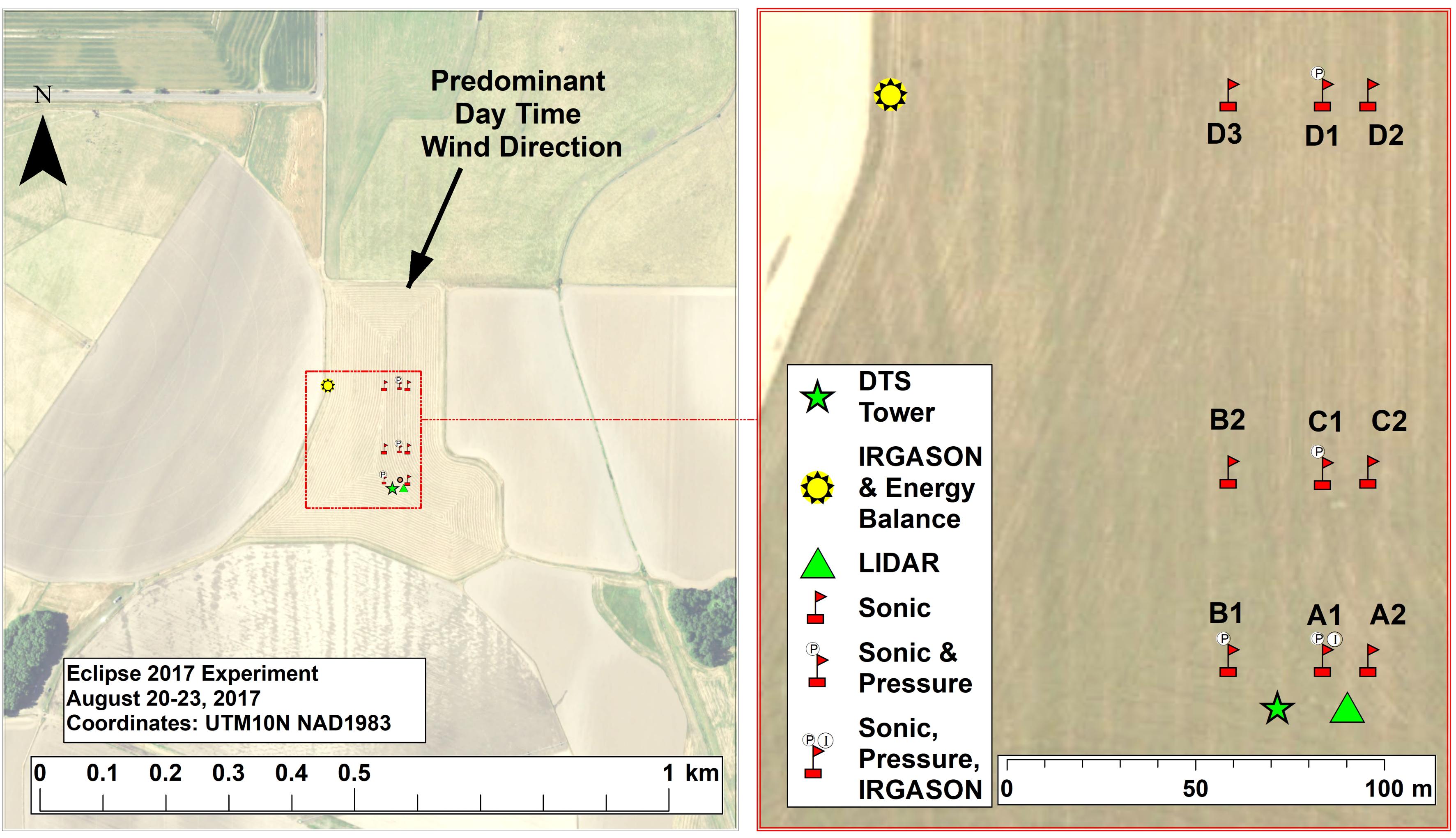
Figure 1. Map and diagram of the experimental layout showing the positions of the instrumentation. The array covered an area of 0.6 ha.

Horizontal Array for Rapid Flux Measurements

A distributed horizontal instrument array containing nine stations with 10 ultrasonic anemometers and four Paroscientific 216B pressure sensors measured fluctuating 3-D wind components [u, v, and w (m s^–1)], pressure [P(hPa)], and temperature [T(°C)]. Precision in ensemble-averaged parameters was maximized by deploying cross-calibrated, identical instruments when measuring a given environmental variable. For example, the 3-D wind components were measured with nine Young 81000 VRE ultrasonic anemometers mounted at the tops of 3-m-tall guy-wired masts (labeled as TOWER in Figure 2) in the logarithmically-spaced pattern shown in Figures 1, 2. The tenth ultrasonic anemometer is a component of an IRGASON (Campbell Scientific) mounted on Tower A1 at 1.56 m a.g.l. and is not used in the analysis herein.

FIGURE 2

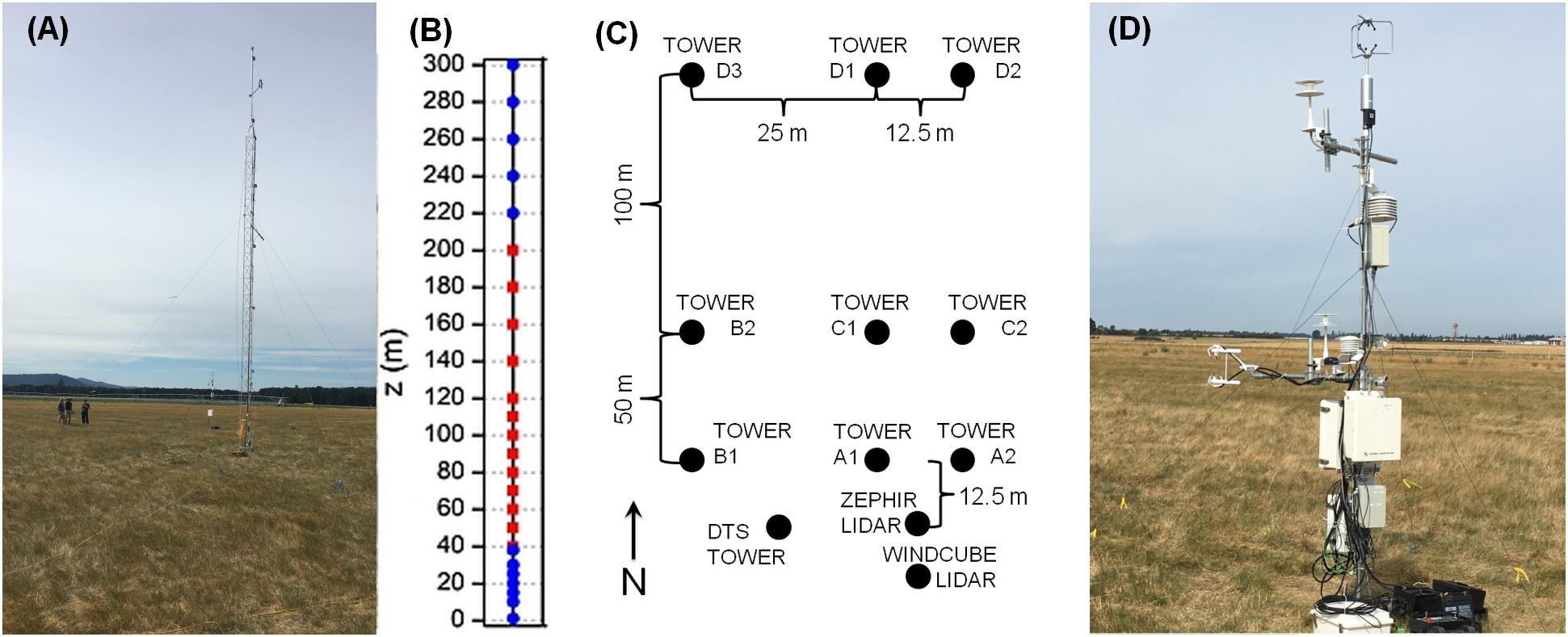
Figure 2. Schematic of the 3-D measurement domain showing (A) a north facing view of the DTS tower, (B) the vertical extent of the domain as a virtual tower with ZephIR300 measurements in blue (circle symbol) and WindCube v2 heights in red (square symbol), (C) the horizontal domain showing the logarithmic spacing of the sonic array, and (D) a photograph of Tower A1.

Young 81000 VRE ultrasonic anemometers are omni-directional and have a 1 cm s^–1 resolution and 5 cm s^–1 accuracy at wind speeds below 30 m s^–1. For convenience, we refer to these nine ultrasonic anemometers as the “sonic array.” After deploying the sonic array, we utilized a custom-built laser alignment tool to align each ultrasonic anemometer to a reference marker placed 50 m due north of each mast’s position. This process was used to ensure that all ultrasonic anemometers were horizontally-level and aligned to the same northerly reference direction. The masts’ positions and the directional alignment target positions were established with an RTK (real-time kinematic) GPS with <3 cm precision. Four Campbell Scientific CR3000 data loggers, located at A1, B1, C1, and D1 (Figures 1, 2), acquired sonic array data at 20 Hz for the entire array and stored the data on flash cards through a Campbell Scientific NL115 ethernet/compact flash module mounted on each logger. Referring to Figures 1, 2, individual ultrasonic anemometers in the experiment array were named after their respective logger designation such that logger A collected data from sonics A1 and A2, logger B collected data from sonics B1 and B2, logger C collected data from sonics C1 and C2 and logger D collected data from sonics D1, D2, and D3.

Each data logger was paired with a dedicated Garmin GPS antenna (Model GPS16x-HVS) that, in concert with software embedded in the logger program, time synchronized the four loggers through GPS signals. The GPS16x-HVS has a 10 μs time accuracy, five times faster than the time between turbulence observations at the 20 Hz sampling rate. The logger was programmed to acquire GPS data and adjust logger clocks at 1 Hz, as recommended by the manufacturer’s data sheet. Two 36 Ah deep cycle batteries were paired with each logger to power the array stations over the observation period encompassing the eclipse.

A Vaisala HMP155 humidity and temperature probe mounted in a passive radiation shield at 2.5 m nominal height was mounted on each mast in the sonic array. HMP155 thermo-hygrometers have an approximate 20 s response time but were oversampled at 20 Hz and data were averaged in post-processing. Each thermo-hygrometer shared the name of the ultrasonic anemometer on a given mast, and thermo-hygrometer data were logged to the respectively-named logger; e.g., thermo-hygrometer A1 was paired with ultrasonic anemometers A1 and data were collected on logger A. These temperature and humidity sensors were calibrated before the experiment deployment by co-locating the instruments and acquiring environmental data over a 24-h period during conditions with a range of temperatures exceeding the temperature range encountered during the eclipse. Linear calibrations yielded R² no less than 0.991 for temperature and no less than 0.90 for humidity.

High-frequency pressure changes in the horizontal plane were captured with shielded Paroscientific 216B pressure sensors mounted on towers A1, B1, and C1 at 3-m nominal height and data were recorded at 20 Hz on data loggers A, B and C, respectively. The pressure shields are designed to minimize the influence of dynamic pressure effects on pressure measurements. The minimal spacing of at least 25 m between pressure sensors was sufficiently distant such that one can discriminate a pressure wave traveling at the speed of sound with a 20 Hz sampling rate. Model 216B pressure sensors are configured to measure pressures in the range 800–1100 hPa with 0.03 Pa precision. Post-experiment, we cross-calibrated the pressure sensors by co-locating them on a lab bench and acquiring atmospheric pressure changes over several days. From these data, we derived linear calibrations between the reference sensor and the remaining sensors with R² no less than 0.996.

Turbulent Flux Averaging

Sensible heat fluxes, H, were calculated from the sonic array with two approaches. First, the sensible heat flux was calculated from each 3-D ultrasonic anemometer independently on a 20-min averaging interval. This 20 to 30 min time-averaging protocol has become standard eddy-covariance practice for idealized, i.e., quasi-stationary and horizontally homogeneous, conditions (Lee et al., 2005; Aubinet et al., 2012). Second, the flux was computed on several shorter time intervals, as short as 15 s, using the synchronized and aligned sonic array. Data from all nine anemometers, within the same time interval, were composited together. Mean velocities and temperatures were calculated in space and time from this composite. The individual, space-time-ensemble (“STE,” hereafter) mean was then subtracted from all nine locations to create a spatial-temporal fluctuating quantity: $T^{″}(\overrightarrow{x},t)=T(\overrightarrow{x},t)-⟨\overline{T}⟩$, where the double prime distinguishes the space-time fluctuations, the overbar represents time averaging, the bracket represents spatial averaging, T is the sonic temperature and $\overrightarrow{x}$ is the position vector for the relative locations of anemometers in the array. Vertical wind velocity (w) perturbations were calculated in an identical manner. Rapid sensible heat fluxes are then calculated accordingly as $H=\mathrm{\rho }{c}_p⟨\overline{w^{″}{T}^{″}}⟩$, where ρ = 1.2 kg m^–3 and c_p = 1000 J kg^–1 K^–1 are the density and specific heat capacity of air, respectively.

Surface Energy Budget Sensors

Located 100 m to the west of the sonic array (Figure 1), an additional 6 m tall tower was instrumented as a joint eddy-covariance and energy budget station for a longer-term field campaign that overlapped the eclipse experiment. Data used for the analyses herein include radiative and ground heat fluxes. Net radiation was measured with a Hukseflux NR01 four-component net radiometer mounted at 3.41 m a.g.l. on the energy budget station. A ground heat flux sensor (Hukseflux HFP01) was installed at 5 cm depth at the station, and a post-processed calibration was calculated for in situ conditions from 1 week (post-experiment) of temperature data collected at 5 and 30 cm depths using Decagon GS3 soil temperature/water content sensors. These sensors were sampled at 1-s intervals, with 1-min averages recorded with a Campbell Scientific CR1000 data logger, which was synchronized with GPS and cell clocks daily to within 1 s of GPS time.

Lidar

A Doppler wind lidar is a remote sensing instrument that measures the wind field. Horizontal and vertical wind speed and wind direction are derived by measuring the backscattered laser beams along a conical, upward facing scan. A set of assumptions about the state of the atmosphere, e.g., horizontal homogeneity in the flow field, are invoked in these calculations. Specific details regarding the lidar-derived wind velocity calculations and the associated assumptions are described extensively in Newsom et al. (2015), Newman et al. (2016), and Choukulkar et al. (2017).

Two vertical-profiling Doppler lidar systems were deployed to observe the wind field response to the eclipse. The first was the WindCube v2 (Leosphere, Orsay, France), a pulsed Doppler lidar that emits regularly spaced emissions of infrared light for a specified pulse length to measure the radial wind speed. During operation, five beams are emitted, four in the cardinal directions (cone half-angle = 28°) and one pointed vertically, at a rate of approximately 4 s to make a complete conical scan. Twelve user-programmable heights within a 40 to 200 m a.g.l. range are available, and each range gate is 20 m in length (i.e., the probe depth). Accuracy for the WindCube v2 is ±0.1 m s^–1 for wind speed and 1.5° for wind direction in flat, homogeneous terrain (Cariou, 2011).

A ZephIR300 (ZephIR Ltd., North Ledbury, United Kingdom) was also deployed to cover other heights of interest, particularly those closer to the ground surface. The ZephIR300 is a coherent continuous-wave lidar capable of measuring the wind field from 10 to 300 m a.g.l. at 10 user-programmed range gates. In contrast to the WindCube v2, the probe depth is not constant, and increases with increasing height above ground level. Probe depth ranges from 1.4 at 10 m a.g.l. to 15.4 at 100 m a.g.l. The ZephIR300 completes a conical scan pattern (1 scan per second per range gate, 50 measurements per scan, cone half-angle = 30°) to compute the radial velocity at each height. Reported accuracy for the ZephIR300 in flat, homogenous terrain is ±0.5% for wind speed and ±0.5° for wind direction (Slinger and Harris, 2012).

These two lidar instruments were used to create a virtual meteorological tower reaching a height of 300 m with 24 heights measured from 10 to 300 m, spaced unevenly such that higher resolution was obtained closer to the surface (see Figure 2B). In addition to the 10 programmable heights, the ZephIR300 has a surface meteorological station capable of measuring wind speed and direction at 1 m and a base height taken at 38 m.

A cross-validation was completed for the two lidar systems at a flat, open field on the Lawrence Livermore National Laboratory (LLNL) campus prior to deployment. During calibration the lidars were deployed alongside a 52-m tall meteorological tower for 28 days. The LLNL calibration tower was equipped with wind vanes (Met One 020C, Met One Instruments, Inc., Grants Pass, OR, United States) and cup anemometers (Met One 010C) at three heights, 10, 23, and 52 m. Very good agreement between measurements of both lidars and the LLNL meteorological tower was found for both wind speed and direction, with R² values ranging from 0.977 (z = 10 m) to 0.999 (z = 100 m) for wind speed and 0.90 (z = 10 m) to 0.999 (z = 100 m) for wind direction.

Distributed Temperature Sensing

High-resolution profiles of the thermal surface layer were obtained with Distributed Temperature Sensing (DTS). DTS systems observe changes in the temperature-dependent Raman scattering of laser light within a fiber-optic cable to resolve the temperature along the cable at high spatial and temporal resolution (12.5 cm in space and 1 s in time). Reviews of the measurement principle can be found in Dakin et al. (1985), Kurashima et al. (1990), Williams et al. (2000), Selker J.S. et al. (2006), Selker J. et al. (2006) and Tyler et al. (2009). The DTS measurement technique has recently been adapted to atmospheric research applications. The flexibility of the fiber-optic system allows for multiple deployment geometries that can be used to observe targeted phenomenon. For example, Higgins et al. (2018) suspended a fiber-optic cable from an unmanned aircraft system (UAS) to observe the morning transition. Thomas et al. (2012) and Zeeman et al. (2015) created quasi three-dimensional arrays of fiber to observe near surface motions in the stable surface layer. Krause et al. (2013) measured the thermal patterns within a forest canopy. Sayde et al. (2015) observed rapid changes in wind speed and temperature across a shallow gully.

An approximately 100-m long section of fiber-optic cable was deployed for the solar eclipse experiment. The fiber was interrogated with an ULTIMA^TM unit (Silixa, Elstree, United Kingdom), which has a sampling resolution of 12.5 cm along the fiber-optic cable, a measurement time resolution of 1 s, and temperature resolution is 0.1°C. The fiber-optic cable was installed such that it passed through two calibration baths before ascending and descending a 15-m tall tower and returning through the initial calibration baths. The fiber-optic cable had a 50 μm glass fiber core surrounded with Kevlar and an outer protective layer of white plastic (outer diameter 0.9 mm). One calibration bath was maintained as an ice and water slurry, the other was kept at ambient temperature. Each water bath was insulated inside a cooler and agitated with aquarium bubblers to reduce thermal stratification. The temperature within each water bath was measured with a platinum thermocouple and an RBRsolo (RBR Ltd., Ottowa, ON, Canada). DTS temperature measurements were calibrated against the reference bath temperatures for each 1-s measurement interval.

Results and Discussion

The 2017 total solar eclipse was observed at a field site along the path of totality in Corvallis, Oregon. The center of maximum totality at the field site was observed on August 21 at 10:17:39 (PDT). The site experienced clear sky conditions for a 48-h period starting the day prior to the eclipse, 20 August 2017, and continuing through the eclipse and into the following evening, 21 August 2017. Smoke from forest fires to the northeast descended upon the area on 22 August 2017, ending the clear sky period.

Time series obtained from the sensor array showing the 2-min STE mean pressure, temperature, and wind speed at 3 m through the clear sky period are presented in Figure 3. Pressure (Figure 3A) was relatively constant throughout the eclipse, though there was a 0.2 hPa decrease in pressure, at the lower limit but consistent with previous observations during an eclipse. We see no evidence of post-eclipse pressure waves observed in other studies (e.g., Goodwin, 1983; Aplin et al., 2016; Zirker, 2016). Temperature measurements (Figure 3B) are consistent between the HMP155 array and the DTS measurements at 3 m elevation. A temperature anomaly of approximately 3°C was observed during the eclipse, consistent with prior observations detailed in section “Introduction.” The observed near-surface temperature anomaly was greater than 79.7% of eclipse observations found in the literature (Table 3, Eugster et al., 2017). During the 2-h interval spanning the eclipse, ground temperature measured with an Apogee infrared radiometer decreased by 10°C before totality and increased by 14°C afterward (not shown). This 12°C-hr^–1 temperature swing exceeds the sunrise heating rate of 2.8°C-hr^–1 and sunset 3.4°C-hr^–1 cooling rate for 2-h time intervals spanning sunrise and sunset during the same day. The 3-m wind speed (Figure 3C) diminished after totality, consistent with previous eclipse measurements (see section “Introduction”) and is characterized by a total change in near-surface wind speed of approximately 2 m s^–1.

FIGURE 3

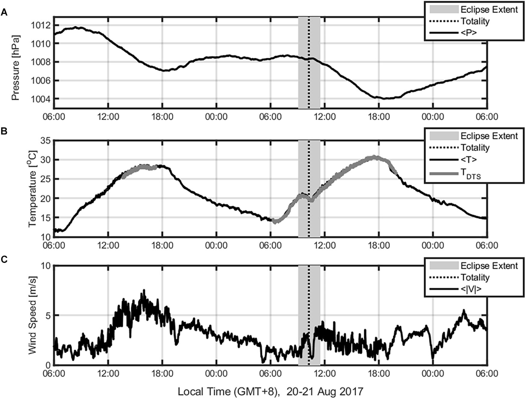
Figure 3. Time series of the 2-min STE mean pressure (A), temperature (B) and wind speed (C) at 3 m elevation through the observation period from the sensor array, and the 2-min mean DTS temperature at the 3-m (a.g.l.) fiber-optic range gate. Sunrise occurred at 06:22 and sunset at 20:08 local time.

A detailed tableau of the near-surface DTS-temperature profile evolution through the eclipse is presented in Figure 4. The near-surface region initially cools faster creating a stable thermal inversion at the surface just prior to totality. After totality, the land surface begins to warm again, and an unstable stratification is reestablished. The eclipse-induced temperature anomaly extends upward through the near-surface measurement region. The peak of the thermal anomaly lags totality and diminishes in magnitude as the height above the land surface increases.

FIGURE 4

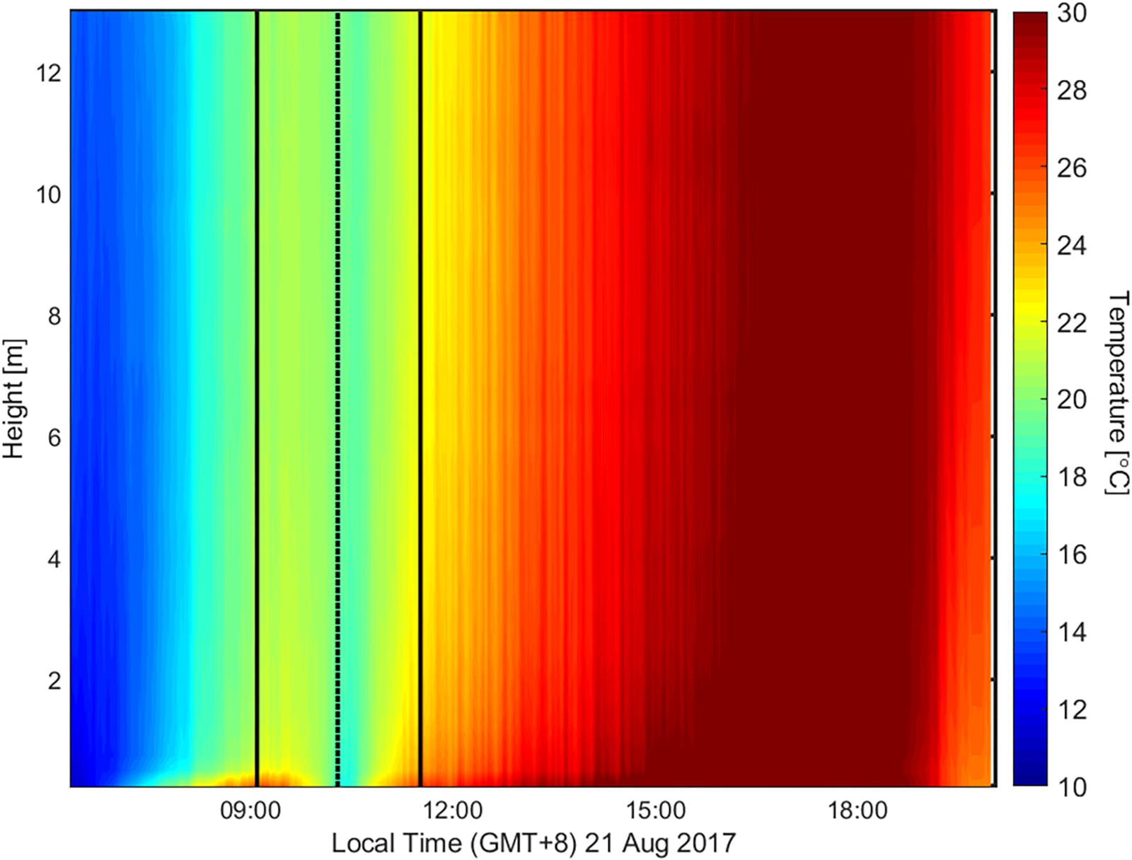
Figure 4. DTS temperature measurements at 1-s time- and 12.5-cm vertical-space-resolution throughout the eclipse depicting the evolution of the near-surface boundary layer.

The eclipse produced changes in wind flow similar to the observed temperature profile in Figure 4. The lidar data show two important trends: 1) a slacking of the wind speed after totality, reaching a maximum decrease of 2.5 m s^–1, and 2) changes in wind speed differ in magnitude and timing according to height, which creates strong wind shear post-totality (Figures 5, 6). The decrease in wind speed was only observed from the surface up to 140 m, as flow above 220 m appears to be fully decoupled from the very-near-surface layer below, as hypothesized by Foken et al. (2001) and observed by Schulz et al. (2017). Below 220 m, the magnitude of the wind speed decrease ranged from 2.5 m s^–1 at 10 m to 1 m s^–1 at 160 m. Unfortunately, the exact height of this decoupling is uncertain due to missing wind speeds from 150 to 200 m caused by a poor signal to noise ratio from the WindCube v2 lidar. Observations in wind direction (not shown) indicate a strong backing of the wind, or counterclockwise rotation below 50 m. A greater than 40° wind shift was observed at 1 m height between 10:30 and 10:40 PST, approximately 15 min lagging totality. This is slightly stronger than the 20°counterclockwise shift observed during the 20 March 2015 solar eclipse over the British Isles (Gray and Harrison, 2016), however, the United Kingdom observation site was only within 85% totality. The counterclockwise rotation shift has been attributed to rapid eclipse-induced cooling analogous to the formation of the transient wind regime at sunset (Gray and Harrison, 2016).

FIGURE 5

Figure 5. Time trace of horizontal wind speed from 1 to 300 m measured by lidar. The data show significant shear following the eclipse which is most pronounced between 30 and 140 m. Note that due to lidar start up errors, the ZephIR300 did not start collecting data until just prior to totality.

FIGURE 6

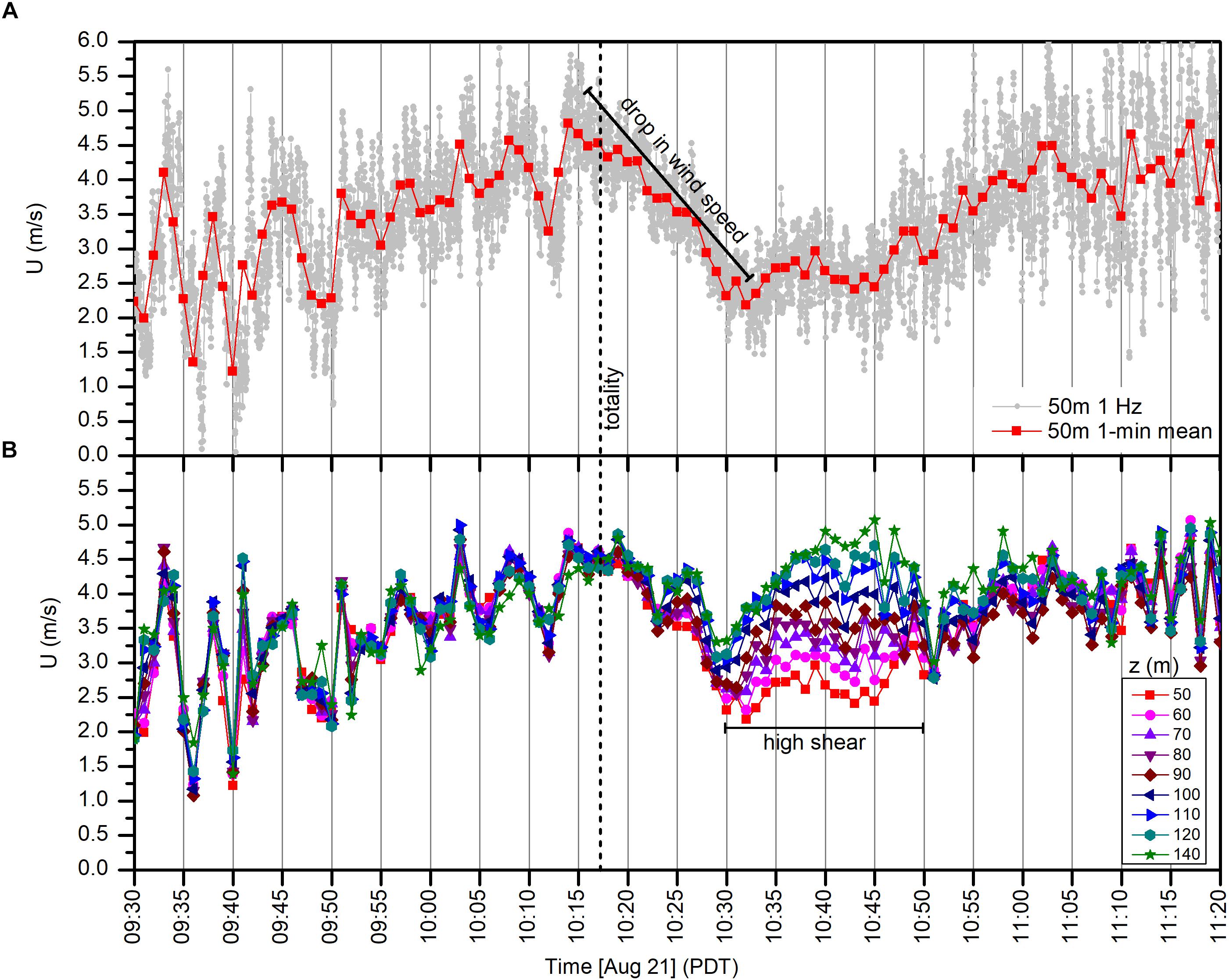
Figure 6. A subset of the lidar data illustrating the time lag between totality, the decrease in wind speed, and maximum shear. (A) Data collected at 50 m including the 1 Hz and 1-min averages of wind speed. (B) 1-min averages for all heights between 50 and 140 m.

To look more closely at the timing and magnitude of the wind response to totality, a subset of the data is plotted in Figure 6. This figure shows that the eclipse-induced decrease in wind speed lasts longer for the heights closest to the surface. High wind shear is apparent for nearly 20 min starting 10 min after totality and a weaker period of shear is apparent 5 min after totality.

Time series of sensible heat fluxes, calculated with standard 20-min time averaging (for individual ultrasonic anemometers), 20-min STE averaging periods and with “rapid” STE averaging (1 or 2-min), are presented in Figure 7A.

FIGURE 7

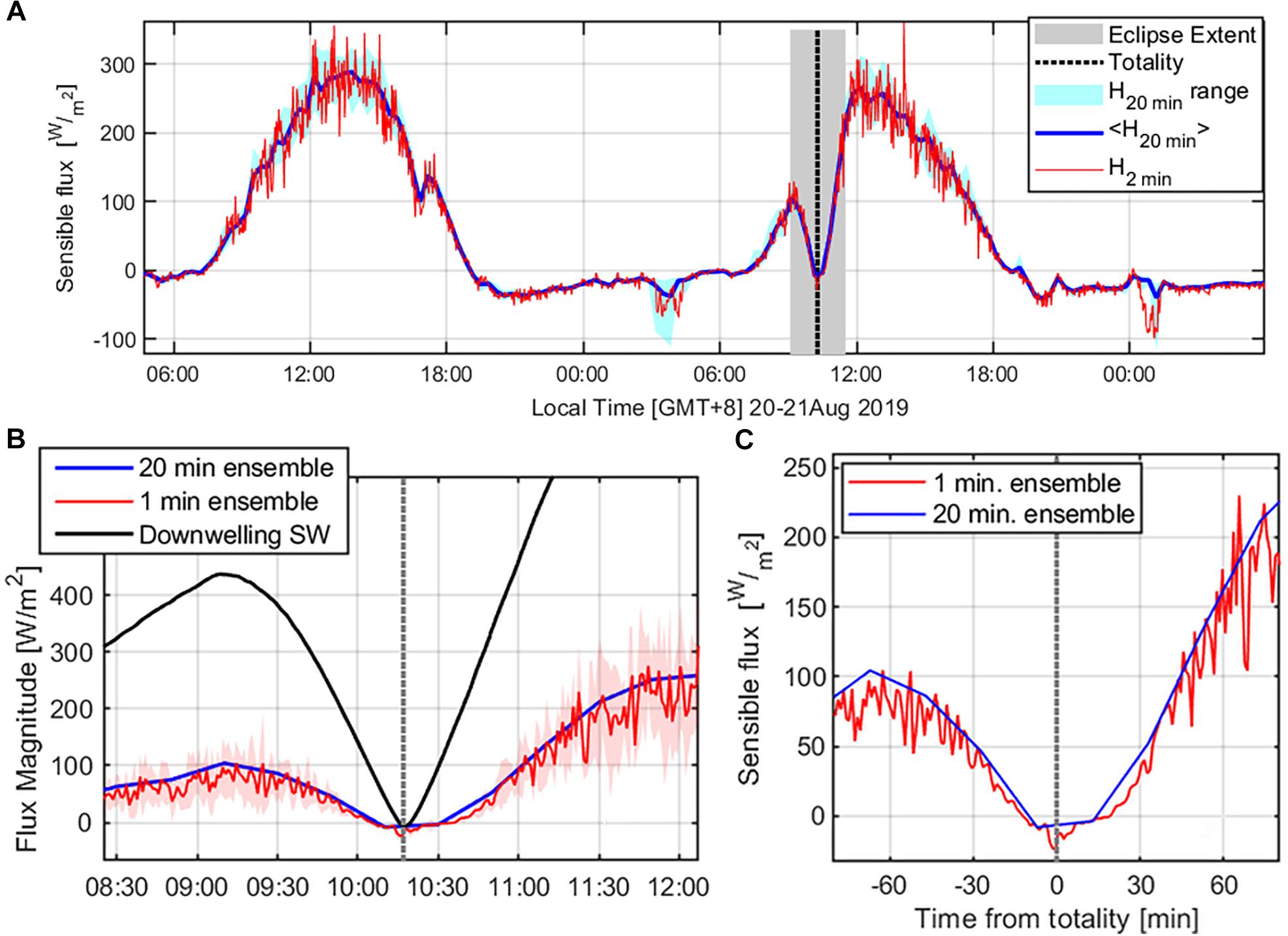
Figure 7. Comparisons between the sensible heat fluxes calculated with the STE averaging over periods of (A) 20 min and 2 min along with the 20-min range from the sonic array; (B) Sensible flux calculated for 20 min and 1 min periods, with ±1 standard deviations of 1 min flux time series (shaded), and the downwelling shortwave (SW) radiation; and (C) 20 min and 1 min sensible flux at 2 h period centered on totality.

In Figure 7, the thick, blue, dashed line shows the 20-min STE mean of the sensible heat fluxes. The cyan shading behind the time trace in Figure 7A is the range between the maximum and minimum of the nine individual 20-min time-averaged flux measurements within that interval. The thin, red line is the “rapid” sensible heat flux calculated from the STE averaging approach, outlined in the previous section, at either 2-min (Figure 7A) or 1-min (Figures 7B,C) time blocks. Throughout the eclipse experiment, the majority of the rapid STE sensible heat flux measurements are within the min-max interval of the nine individual, slow (20-min) flux measurements. Note that times of major disagreement (i.e., a large range in the 20-min sensible heat fluxes) occur at night under stable conditions. These discrepancies occur when a highly-localized cold air mass penetrates only a portion or the array, leading to large spatial gradients (not shown), and corresponding to large negative heat fluxes. These fluxes are not a result of turbulent motions but rather sub-meso motions of the non-equilibrium stable boundary layer (Mahrt, 2010) that are not typically distinguishable with longer (20-min) time averaging and standard eddy-covariance methods (Mahrt, 2009).

The rapid STE flux approach (Figures 7B,C) also has a stronger response to the very rapid changes occurring around peak totality (at the local minimum in downwelling shortwave radiation in Figures 7B,C, noted by a vertical line in Figure 7C). This is expected and illustrates that the rapid STE approach is capable of capturing fluctuations in the surface exchanges that are not resolvable with the standard implementation of eddy-covariance over 20-min averaging periods. A zoomed-in image of the sensible heat flux behavior through the eclipse is presented in Figure 7C. At totality, the flux rapidly decreased to a minimum of −30 W m^–2. Following totality, the sensible heat flux magnitude increased exponentially to neutral stratification (H = 0) over a span of approximately 20 min (the approximate time-averaging scale for most eddy-covariance measurements), and then entered a new recovery phase. The 20-min STE averaged flux measurements do capture a small negative sensible heat flux at the time of totality, but do not reveal the behavioral evolution of rapid decline and recovery nor the full flux magnitude (underestimating it by about 20 W m^–2).

Bias is a major concern for any turbulent flux measurements over relatively short averaging periods as the tendency of a rapid approach would be to not capture contributions of larger-scale motions to the overall land-surface flux. If these larger-scale motions were not captured, the fluxes calculated by the new rapid-STE approach would have a systematic bias or underestimation of the full flux magnitude as calculated by standard methods with longer time averages. The difference between the mean of the nine independent flux measurements and the flux estimated with the rapid spatial-temporal approach is quantified in Figure 8A. The STE fluxes calculated on 20-min averaging times are linearly interpolated so that they can be compared with the fast flux measurements. In all cases, the median bias is negative and less than 2 W m^–2 in magnitude.

FIGURE 8

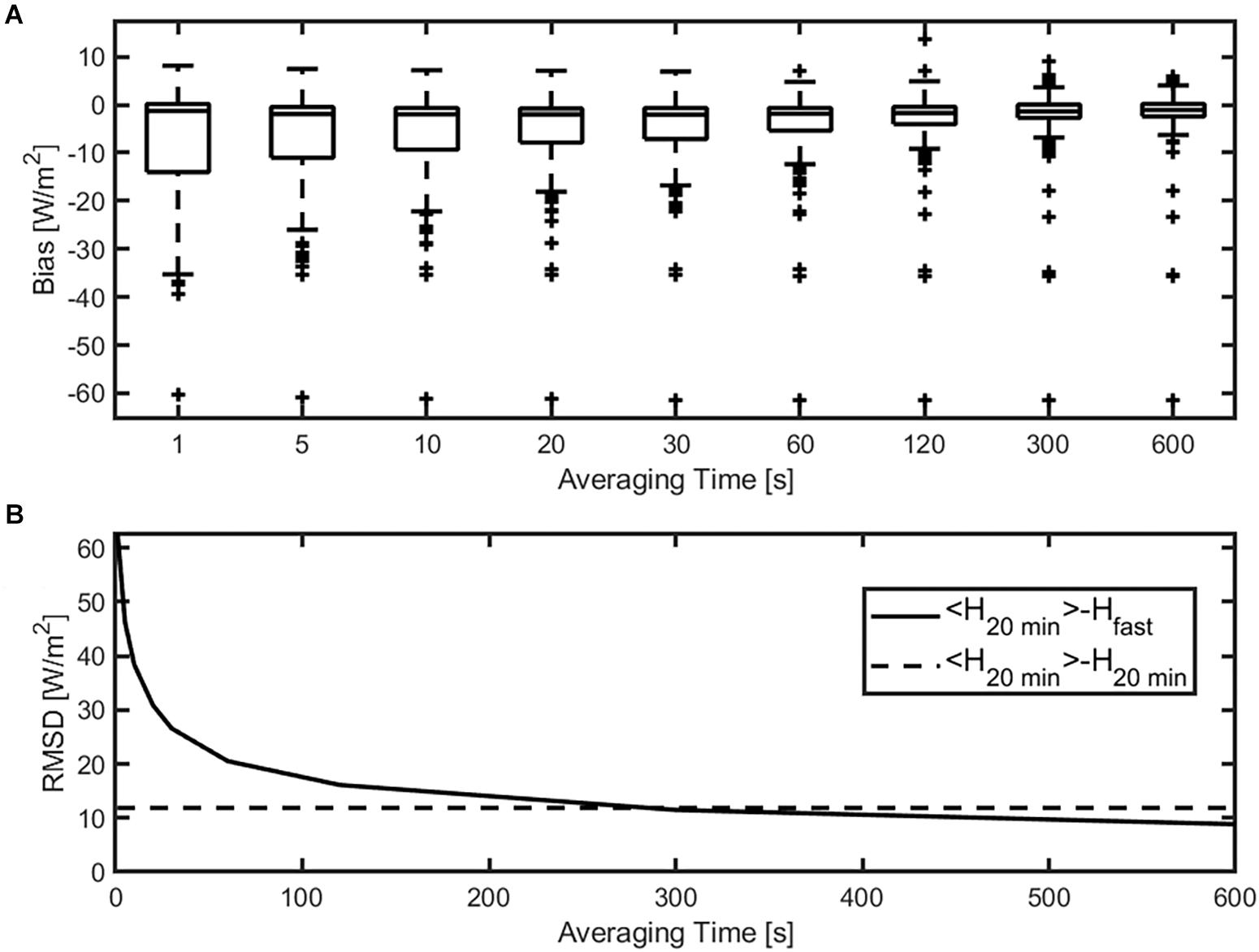
Figure 8. Quantitative comparisons of STE averaging times for (A) bias and (B) root-mean-square difference (RMSD).

The root mean squared difference (RMSD) between the mean of the nine independent flux measurements and the rapid STE approach is presented in Figure 8B. Here, the RMSD decreases as the fast flux averaging time interval increases. The horizontal reference line is the RMSD of the nine independently calculated 20-min flux measurements about their mean. The STE averaged RMSD crosses below this threshold at the 5-min averaging interval. Note that the RMSD between the 20-min flux and the rapid STE flux measurement does not necessarily represent error between methods.

Figure 9 presents an analysis we used to characterize how quickly the atmosphere responds to the eclipse perturbation. It shows the 1-min STE sensible heat flux response to rapidly changing insolation and the exponential recovery (Figure 9) from the most negative heat flux peak to the no net flux (H = 0 Wm^–2) condition. The exponential recovery exhibits a time-constant of 0.146, corresponding to an e-folding time of 6.85 min. This order 10-min (or less) timescale characterizes how rapidly the atmosphere responds to the perturbation of available energy at the land surface.

FIGURE 9

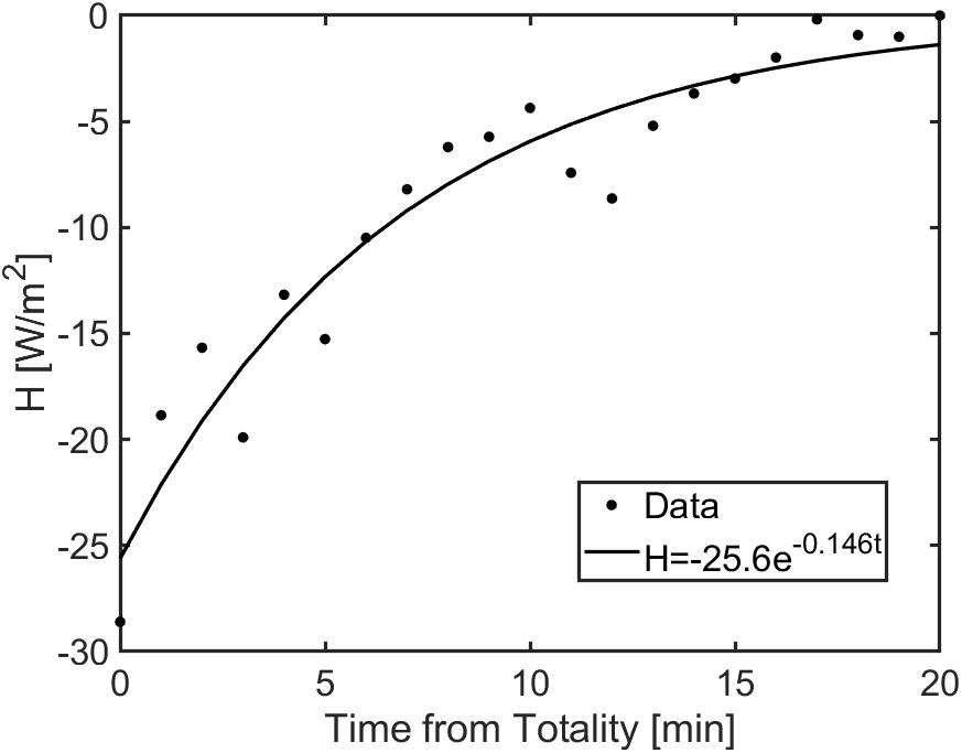
Figure 9. The 1-min STE sensible heat flux response and recovery time scale analysis.

To reconcile this observed time response in the sensible heat flux with time response in available energy, i.e., the net radiation and ground heat flux (Rn - G), lagged cross-correlations were calculated between the two energy terms. The rapid fluctuation of each component was tabulated by subtracting the 20-min running average flux magnitude from the flux measured over 1-min periods (i.e., $H^{\prime }=⟨{\overline{H}}_{1\mathrm{𝑚𝑖𝑛}}⟩-⟨{\overline{H}}_{20\mathrm{𝑚𝑖𝑛}}⟩$), similar to a Reynold’s decomposition. Lagged cross-correlations were found between fluctuations in each component, at intervals of 1-min time lags up to a maximum of 6 h (360 lagged intervals), although we present results only for ±25-min lags (Figure 10).

FIGURE 10

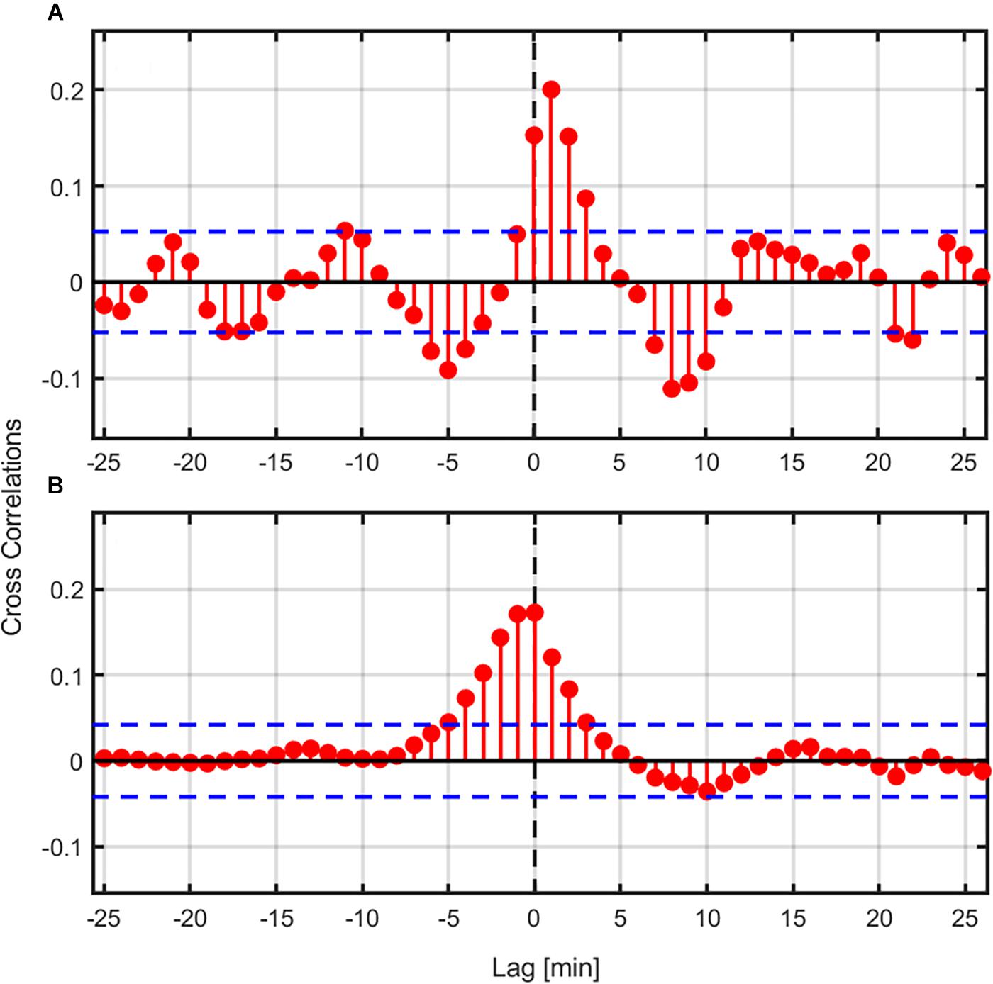
Figure 10. Cross-correlations between 1-min fluctuations in the source terms [(Rn - G)′] and turbulent heat flux (H′) (A) during sunlit periods (Rn > 5 W m^–2), and (B) during dark periods (Rn < 5 W m^–2). Dark periods include the time near totality, as well as nighttime periods. Blue lines indicate the approximate 95% confidence interval.

This cross-correlation analysis (Figure 10) shows that coupling is evident between the vector sum of net radiation and ground heat flux (Rn - G) and the 1-min STE heat flux determined array ensemble. Coupling between the available energy (Rn - G) and the turbulent flux can be conditionally differentiated by sunlit (Rn > 5 W m^–2 in Figure 10A) and dark (Rn < 5 W m^–2 in Figure 10B) periods (daytime and either nighttime or near totality, respectively). While incoming solar radiation is heating the surface (Rn > 5 W m^–2 in Figure 10A), the concurrent instability is indicated by a cross-correlation that peaks at a 1-min lag, and rapidly drops off below the 95% confidence interval after 3-min of lag. During dark periods (Rn < 5 W m^–2 in Figure 10B), when stable conditions dominate and there is no net source term for surface heating, positive correlations occur over a broader range of lag and are centered at negative but near-zero time lags. This may indicate that over short periods without solar forcing (primarily at night), small fluctuations in near-surface heat exchange are affected by temperature gradients induced by slow sub-meso scale motions, in addition to upwelling, long-wave radiative flux.

These correlations indicate that linkages across the energy pathways are measurable even over short time intervals. They also indicate that atmospheric response times are on the order of 10 min or less, which agrees with the exponential time-response analysis (Figure 9). In general, a lack of closure in the surface energy budget might be related to differences in time response for the various flux components, corresponding to the often-cited problem of advective flux divergence (Foken, 2008; Leuning et al., 2012).

Conclusion

We conducted a field experiment during the 2017 total solar eclipse in Corvallis, Oregon aimed at observing the near-surface atmospheric response to the rapid change in solar radiative forcing. We observed much of the expected eclipse-induced behavior in mean temperature, pressure and wind velocity (Figures 3–6). Specifically, rapid changes in air temperature, wind dynamics and surface flux dynamics were recorded. These temperature and wind measurements were consistent with previous surface station measurements. Compared to previous studies, we expanded the vertical extent of observations through the use of lidar and DTS techniques. Lidar measurements indicate a decoupling from the surface that resembles a smaller-scale nocturnal residual layer aloft with stable stratification and weak winds closer to the surface, which generate strong wind shear (Figures 4–6).

The eclipse provided a unique opportunity to develop and test new rapid methods for surface flux measurement during non-equilibrium events. These methods employed a turbulent flux sensor array, designed to measure both the small (short) and large (long) scales of turbulent fluctuations that contribute to the integrated surface heat flux. Given a sufficiently dense array, our results suggest that flux can be measured over periods shorter than 1 min. The new method presented was able to measure sensible heat fluxes with less than 2 W m^–2 median bias for periods as short as 15 s. Our observations with this new technique indicate that the atmosphere responds rapidly to changes in the available energy at the land surface, and that these types of rapid fluctuations in sensible heat flux may be common and perhaps unobserved, particularly at night. We showed that resolving rapid changes in turbulent fluxes corroborate previous estimates of atmospheric response time. Finally, these rapid flux estimates facilitate cross-correlation analyses between linked energy pathways, such that time lags between key quantities (e.g., terms in the energy balance equation) can be investigated.

These independent analyses indicated that the atmosphere responds to rapid changes in surface forcing over a time scale of 10 min or less. The spatial-temporal-ensemble (STE) surface flux measurement technique could also be used to verify and test other rapid flux algorithms. The approach may also provide a means to link the flux response to relatively larger-scale atmospheric motions and events (e.g., sub-meso scale motions). This would provide a new basis for atmospheric scaling of non-stationary flux at the land surface.

Author Contributions

All authors participated in the experimental design, experimental execution, data collection and edited the manuscript. CH, JK, and SW prepared the figures.

Conflict of Interest Statement

The authors declare that the research was conducted in the absence of any commercial or financial relationships that could be construed as a potential conflict of interest.

Acknowledgments

The authors are grateful for the support of our students and staff who made the field experiment possible: Jack Blackman, Taylor Vagher, Johanna Alexson, Hadi Al-Agele, and Alex Krejci. Green springs Farms generously allowed access to their land for the field experiment. Additional material support was provided by the lab of Drs. Anne Nolin and Simon de Szoke (OR, United State), and by the Lawrence Livermore National Laboratory, operated by Lawrence Livermore National Security, LLC, for the United States Department of Energy, National Nuclear Security Administration under Contract DE-AC52-07NA27344.

References

Anderson, R. C., and Keefer, D. R. (1975). Observation of the temperature and pressure changes during the 30 June 1973 Solar Eclipse. J. Atmos. Sci. 32, 228–231. doi: 10.1175/1520-0469(1975)032<0228:oottap>2.0.co;2

CrossRef Full Text | Google Scholar

Anfossi, D., Schayes, G., Degrazia, G., and Goulart, A. (2004). Atmospheric turbulence decay during the solar total eclipse of 11 August 1999. Bound. Layer Meteorol. 111, 301–311. doi: 10.1023/B:BOUN.0000016491.28111.43

CrossRef Full Text | Google Scholar

Antonia, R. A., Chambers, A. J., Phong-Anant, D., Rajagopalan, S., and Sreenivasan, K. R. (1979). Response of atmospheric surface layer turbulence to a partial solar eclipse. J. Geophys. Res. Oceans 84, 1689–1692. doi: 10.1029/JC084iC04p01689

CrossRef Full Text | Google Scholar

Aplin, K. L., and Harrison, R. G. (2003). Meteorological effects of the eclipse of 11 August 1999 in cloudy and clear conditions. Proc. R. Soc. AMath. Phys. Eng. Sci. 459, 353–371. doi: 10.1098/rspa.2002.1042

CrossRef Full Text | Google Scholar

Aplin, K. L., Scott, C. J., and Gray, S. L. (2016). Atmospheric changes from solar eclipses. Philos. Trans. R. Soc. Math. Phys. Eng. Sci. 374:20150217. doi: 10.1098/rsta.2015.0217

PubMed Abstract | CrossRef Full Text | Google Scholar

Aubinet, M., Vesala, T., and Papale, D. (eds) (2012). Eddy Covariance: A Practical Guide to Measurement and Data Analysis. Dordrecht: Springer, doi: 10.1007/978-94-007-2351-1

CrossRef Full Text | Google Scholar

Cariou, J.-P. (2011). “Pulsed lidars, in remote sensing for wind energy,” in Risø Report Risø-I-3184(EN), Risø National Laboratory for Sustainable Energy, eds A. Peña and C. B. Hasager (Roskilde: Technical University of Denmark) 65–81.

Google Scholar

Chimonas, G., and Hines, C. O. (1970). Atmospheric gravity waves induced by a solar eclipse. J. Geophys. Res. 75:875. doi: 10.1029/JA075i004p00875

CrossRef Full Text | Google Scholar

Choukulkar, A., Brewer, W. A., Sandberg, S. P., Weickmann, A., Bonin, T. A., Hardesty, R. M., et al. (2017). Evaluation of single and multiple Doppler lidar techniques to measure complex flow during the XPIA field campaign. Atmos. Meas. Tech. 10, 247–264. doi: 10.5194/amt-10-247-2017

CrossRef Full Text | Google Scholar

Clayton, H. H. (1901). The eclipse cyclone, the diurnal cyclones, and the cyclones and anticyclones of temperate latitudes. Q. J. R. Meteorol. Soc. 27, 269–292. doi: 10.1002/qj.49702712004

CrossRef Full Text | Google Scholar

Dakin, J. P., Pratt, D. J., Bibby, G. W., and Ross, J. N. (1985). Distributed optical fibre Raman temperature sensor using a semiconductor light source and detector. Electron. Lett. 21, 569–570. doi: 10.1049/el:19850402

CrossRef Full Text | Google Scholar

Eaton, F. D., Hines, J. R., Hatch, W. H., Cionco, R. M., Byers, J., Garvey, D., et al. (1997). Solar eclipse effects observed in the planetary boundary layer over a desert. Bound. Layer Meteorol. 83, 331–346. doi: 10.1023/A:1000219210055

CrossRef Full Text | Google Scholar

Eckermann, S. D., Broutman, D., Stollberg, M. T., Ma, J., McCormack, J. P., and Hogan, T. F. (2007). Atmospheric effects of the total solar eclipse of 4 December 2002 simulated with a high-altitude global model. J. Geophys. Res. Atmos. 112:D14105. doi: 10.1029/2006JD007880

CrossRef Full Text | Google Scholar

Eugster, W., Emmel, C., Wolf, S., Buchmann, N., McFadden, J. P., and Whiteman, C. D. (2017). Effects of vernal equinox solar eclipse on temperature and wind direction in Switzerland. Atmos. Chem. Phys. 17, 14887–14904. doi: 10.5194/acp-17-14887-12017

CrossRef Full Text | Google Scholar

Foken, T. (2008). The energy balance closure problem: an overview. Ecol. Appl. 18, 1351–1367. doi: 10.1890/06-0922.1

PubMed Abstract | CrossRef Full Text | Google Scholar

Foken, T., Wichura, B., Klemm, O., Gerchau, J., Winterhalter, M., and Weidinger, T. (2001). Micrometeorological measurements during the total solar eclipse of August 11, 1999. Meteorol. Zeitschrift 10, 171–178. doi: 10.1127/0941-2948/2001/0010-0171

CrossRef Full Text | Google Scholar

Founda, D., Melas, D., Lykoudis, S., Lisaridis, I., Gerasopoulos, E., Kouvarakis, G., et al. (2007). The effect of the total solar eclipse of 29 March 2006 on meteorological variables in Greece. Atmos. Chem. Phys. 7, 5543–5553. doi: 10.5194/acp-7-5543-2007

CrossRef Full Text | Google Scholar

Goodwin, G. L. (1983). Atmospheric gravity wave production for the total eclipse of 11 June 1983. J. Atmos. Terr. Phys. 45, 273–274. doi: 10.1016/S0021-9169(83)80049-X

CrossRef Full Text | Google Scholar

Goodwin, G. L., and Hobson, G. J. (1978). Atmospheric gravity waves generated during a solar eclipse. Nature 275, 109–111. doi: 10.1038/275109a0

CrossRef Full Text | Google Scholar

Gray, S. L., and Harrison, R. G. (2016). Eclipse-induced wind changes over the British Isles on the 20 March 2015. Philos. Trans. A Math. Phys. Eng. Sci. 374:20150224. doi: 10.1098/rsta.2015.0224

PubMed Abstract | CrossRef Full Text | Google Scholar

Harrison, R. G., and Hanna, E. (2016). The solar eclipse: a natural meteorological experiment. Philos. Trans. A Math. Phys. Eng. Sci. 374:20150225. doi: 10.1098/rsta.2015.0225

PubMed Abstract | CrossRef Full Text | Google Scholar

Higgins, C. W., Wing, M. G., Kelley, J., Sayde, C., Burnett, J., and Holmes, H. A. (2018). A high resolution measurement of the morning ABL transition using distributed temperature sensing and an unmanned aircraft system. Environ. Fluid Mech. 18, 683–693. doi: 10.1007/s10652-017-9569-9561

CrossRef Full Text | Google Scholar

Kastendeuch, P. P., Najjar, G., Colin, J., Luhahe, R., and Bruckmann, F. (2016). Effects of the 20 March 2015 solar eclipse in Strasbourg. France Weather 71, 55–62. doi: 10.1002/wea.2673

CrossRef Full Text | Google Scholar

Kimball, H. H., and Fergusson, S. P. (1919). Influence of the solar eclipse of june 8, 1918, upon-radiation and other meteorological elements. Mon. Weather Rev. 47, 5–16. doi: 10.1175/1520-0493(1919)47<5:iotseo>2.0.co;2

CrossRef Full Text | Google Scholar

Krause, S., Taylor, S. L., Weatherill, J., Haffenden, A., Levy, A., Cassidy, N. J., et al. (2013). Fibre-optic distributed temperature sensing for characterizing the impacts of vegetation coverage on thermal patterns in woodlands. Ecohydrology 6, 754–764. doi: 10.1002/eco.1296

CrossRef Full Text | Google Scholar

Kurashima, T., Horiguchi, T., and Tateda, M. (1990). Distributed-temperature sensing using stimulated Brillouin scattering in optical silica fibers. Opt. Lett. 15, 1038–1040. doi: 10.1364/OL.15.001038

PubMed Abstract | CrossRef Full Text | Google Scholar

Lee, X., Massman, W., and Law, B. (eds) (2005). Handbook of Micrometeorology. Dordrecht: Springer, doi: 10.1007/1-4020-2265-4

CrossRef Full Text | Google Scholar

Leuning, R., van Gorsel, E., Massman, W. J., and Isaac, P. R. (2012). Reflections on the surface energy imbalance problem. Agric. For. Meteorol. 156, 65–74. doi: 10.1016/j.agrformet.2011.12.002

CrossRef Full Text | Google Scholar

Mahrt, L. (2009). Characteristics of submeso winds in the stable boundary layer. Bound. Layer Meteorol. 130, 1–14. doi: 10.1007/s10546-008-9336-9334

CrossRef Full Text | Google Scholar

Mahrt, L. (2010). Variability and maintenance of turbulence in the very stable boundary layer. Bound. Layer Meteorol. 135, 1–18. doi: 10.1007/s10546-009-9463-9466

CrossRef Full Text | Google Scholar

McInerney, J. M., Marsh, D. R., Liu, H.-L., Solomon, S. C., Conley, A. J., and Drob, D. P. (2018). Simulation of the 21 August 2017 solar eclipse using the whole atmosphere community climate Model-eXtended. Geophys. Res. Lett. 45, 3793–3800. doi: 10.1029/2018GL077723

CrossRef Full Text | Google Scholar

Newman, J. F., Bonin, T. A., Klein, P. M., Wharton, S., and Newsom, R. K. (2016). Testing and validation of multi-lidar scanning strategies for wind energy applications. Wind Energy 19, 2239–2254. doi: 10.1002/we.1978

CrossRef Full Text | Google Scholar

Newsom, R. K., Berg, L. K., Shaw, W. J., and Fischer, M. L. (2015). Turbine-scale wind field measurements using dual-Doppler lidar. Wind Energy 18, 219–235. doi: 10.1002/we.1691

PubMed Abstract | CrossRef Full Text | Google Scholar

Raman, S., Boone, P., and Shankar Rao, K. (1990). Observations and numerical simulation of the evolution of the tropical planetary boundary layer during total solar eclipses. Atmos. Environ. Part Gen. Top. 24, 789–799. doi: 10.1016/0960-1686(90)90279-V

CrossRef Full Text | Google Scholar

Ratnam, M. V., Kumar, M. S., Basha, G., Anandan, V. K., and Jayaraman, A. (2010). Effect of the annular solar eclipse of 15 January 2010 on the lower atmospheric boundary layer over a tropical rural station. J. Atmos. Sol. Terr. Phys. 72, 1393–1400. doi: 10.1016/j.jastp.2010.10.009

CrossRef Full Text | Google Scholar

Sayde, C., Thomas, C. K., Wagner, J., and Selker, J. (2015). High-resolution wind speed measurements using actively heated fiber optics. Geophys. Res. Lett. 42, 10064–10073. doi: 10.1002/2015GL066729

CrossRef Full Text | Google Scholar

Schulz, A., Schaller, C., Maturilli, M., Boike, J., Ritter, C., and Foken, T. (2017). Surface energy fluxes during the total solar eclipse over Ny-Ålesund, Svalbard, on 20 March 2015. Meteorol. Zeitschrift 26, 431–440. doi: 10.1127/metz/2017/0846

CrossRef Full Text | Google Scholar

Selker, J. S., Thévenaz, L., Huwald, H., Mallet, A., Luxemburg, W., van de Giesen, N., et al. (2006). Distributed fiber-optic temperature sensing for hydrologic systems. Water Resour. Res. 42:W12202. doi: 10.1029/2006WR005326

CrossRef Full Text | Google Scholar

Selker, J., van de Giesen, N., Westhoff, M., Luxemburg, W., and Parlange, M. B. (2006). Fiber optics opens window on stream dynamics. Geophys. Res. Lett. 33:L24401. doi: 10.1029/2006GL027979

CrossRef Full Text | Google Scholar

Slinger, C., and Harris, M. (2012). “Introduction to continuous-wave Doppler lidar,” in Proceedings of the Summer School in Remote Sensing for Wind Energy, Boulder, 32.

Google Scholar

Stewart, R. B., and Rouse, W. R. (1974). Radiation and energy budgets at an arctic site during the solar eclipse of July 10, 1972. Arct. Alp. Res. 6, 231–236. doi: 10.2307/1550088

CrossRef Full Text | Google Scholar

Stull, R. B. (ed.) (1988). An Introduction to Boundary Layer Meteorology. Dordrecht: Springer, doi: 10.1007/978-94-009-3027-8

CrossRef Full Text | Google Scholar

Thomas, C. K., Kennedy, A. M., Selker, J. S., Moretti, A., Schroth, M. H., Smoot, A. R., et al. (2012). High-Resolution fibre-optic temperature sensing: a new tool to study the two-dimensional structure of atmospheric surface-layer flow. Bound. Layer Meteorol. 142, 177–192. doi: 10.1007/s10546-011-9672-9677

CrossRef Full Text | Google Scholar

Turner, D. D., Wulfmeyer, V., Behrendt, A., Bonin, T. A., Choukulkar, A., Newsom, R. K., et al. (2018). Response of the land-atmosphere system over north-central oklahoma during the 2017 Eclipse. Geophys. Res. Lett. 45, 1668–1675. doi: 10.1002/2017GL076908

CrossRef Full Text | Google Scholar

Tyler, S. W., Selker, J. S., Hausner, M. B., Hatch, C. E., Torgersen, T., Thodal, C. E., et al. (2009). Environmental temperature sensing using Raman spectra DTS fiber-optic methods. Water Resour. Res. 45:W00D23. doi: 10.1029/2008WR007052

PubMed Abstract | CrossRef Full Text | Google Scholar

Williams, G. R., Brown, G., Hawthorne, W., Hartog, A. H., and Waite, P. C. (2000). Distributed temperature sensing (DTS) to characterize the performance of producing oil wells. Indus. Sens. Syst. 4202, 39–55. doi: 10.1117/12.411726

CrossRef Full Text | Google Scholar

Zeeman, M. J., Selker, J. S., and Thomas, C. K. (2015). Near-Surface motion in the nocturnal, stable boundary layer observed with fibre-optic distributed temperature sensing. Bound. Layer Meteorol. 154, 189–205. doi: 10.1007/s10546-014-9972-9979

CrossRef Full Text | Google Scholar

Zirker, J. B. (2016). Total Eclipses of the Sun. Expanded Edition. Princeton, NJ: Princeton University Press.

Google Scholar