Anticipated Improvements to River Surface Elevation Profiles From the Surface Water and Ocean Topography Mission

Existing publicly available digital elevation models (DEMs) provide global-scale data but are often not precise enough for studying processes that depend on small-scale topographic features in rivers. For example, slope breaks and knickpoints in rivers can be important in understanding tectonic processes, and riffle-pool structures are important drivers of riverine ecology. More precise data (e.g., lidar) are available in some areas, but their spatial extent limits large-scale research. The upcoming Surface Water and Ocean Topography (SWOT) satellite mission is planned to launch in 2021 and will provide measurements of elevation and inundation extent of surface waters between 78^∘ north and south latitude on average twice every 21 days. We present a novel noise reduction method for multitemporal river water surface elevation (WSE) profiles from SWOT that combines a truncated singular value decomposition and a slope-constrained least-squares estimator. We use simulated SWOT data of 85–145 km sections of the Po, Sacramento, and Tanana Rivers to show that 3–12 months of simulated SWOT data can produce elevation profiles with mean absolute errors (MAEs) of 5.38–12.55 cm at 100–200 m along-stream resolution. MAEs can be reduced further to 4–11 cm by averaging all observations. The average profiles have errors much lower than existing DEMs, allowing new advances in riverine research globally. We consider two case studies in geomorphology and ecology that highlight the scientific value of the more accurate in-river DEMs expected from SWOT. Simulated SWOT elevation profiles for the Po reveal convexities in the river longitudinal profile that are spatially coincident with the upward projection of blind thrust faults that are buried beneath the Po Plain at the northern termination of the Apennine Mountains. Meanwhile, simulated SWOT data for the Sacramento River reveals locally steep sections of the river profile that represent important habitat for benthic invertebrates at a spatial scale previously unrecognizable in large-scale DEMs presently available for this river.

Introduction

Accurate measurements of river water surface elevation (WSE) and slope at fine spatial scales are useful for monitoring river discharge (LeFavour and Alsdorf, 2005), calculating stream power in erosional models (Whipple and Tucker, 1999), interpreting underlying geology (Schumm, 1986), identifying knickpoints (Hayakawa and Oguchi, 2006), and characterizing habitat fragmentation for freshwater fish (Dias et al., 2013). In addition, water surface slope is a good predictor of physical habitat classifications (Jowett, 1993), which have different abundances and compositions of benthic taxa (Brown and Brussock, 1991). In situ stream gauges provide high-accuracy measurements of water elevations at discrete points but lack spatial continuity. Even in the most heavily montiored parts of the world, the gauge network is sparse and becoming sparser (Hannah et al., 2011). This problem is worse in less developed areas like the Arctic (Shiklomanov et al., 2002). Meanwhile, existing global DEMs are insufficient over open water due to missing data, large vertical errors, coarse spatial resolution, or limited temporal resolution (Alsdorf et al., 2007).

Remotely sensed measurements of river surface elevation have been made using a variety of methods that each have their limitations (Schumann and Domeneghetti, 2016). GEOSAT, a radar altimeter launched by the U.S. Navy in 1985, was shown to have root mean square error (RMSE) of 0.7 m compared to gauge stations on the Amazon River (Koblinsky et al., 1993). The TOPEX/Poseidon altimeter was designed to measure ocean topography but is also able to observe rivers with widths larger than 1 km with RMSE of 1.1 m (Birkett et al., 2002). The Jason-2 radar altimeter, part of the Jason series succeeding TOPEX/Poseidon, has been shown to have standard errors of 0.28 and 0.19 m over the Ganga and Brahmaputra rivers, respectively, but, like its predecessors, works best in rivers more than a kilometer wide (Papa et al., 2012). Satellite altimeters can provide high-accuracy WSE measurements, but with relatively poor spatial resolution compared to imaging radars. On the other hand, airborne laser altimeters have been used to map WSEs at high spatial resolution. For example, Biron et al. (2013) found elevation errors with standard deviation of 25 cm at 20 m spatial resolution compared to differential GPS measurements. The Shuttle Radar Topography Mission (SRTM) C-band DEM has an estimated standard deviation of error of 5.5 m for open water and has extensive missing data because radar returns depend on the surface roughness (LeFavour and Alsdorf, 2005). TanDEM-X is a relatively new 12 m resolution global DEM from the German space agency (DLR), but it performs poorly over water for similar reasons to SRTM. As a result, the elevations for many northern latitude water bodies in TanDEM-X are collected during winter months when they are ice covered (Wendleder et al., 2013). The Japanese space agency (JAXA) released the ASTER Global DEM Version 2 in 2011, but water elevations are often missing due to failure of the stereo matching technique method over water (Tachikawa et al., 2011). ArcticDEM is a 2 m resolution photogrammetry-derived digital surface model that covers latitudes north of 60° plus the Kamchatka peninsula and all of Alaska¹. Despite the challenges of photogrammetry over water, extracting elevations from the shoreline on the Tanana River produced an elevation profile with height error standard deviation of 0.30 m at 100 m resolution based on ArcticDEM (Dai et al., 2018). More precise data are available from national elevation products like the National Elevation Dataset (NED) in the United States (Gesch et al., 2002), and TINITALY in Italy (Tarquini et al., 2011), but their limited spatial extent prevents global-scale studies. The Multi-Error-Removed Improved-Terrain (MERIT) DEM is created from SRTM, AW3D30, and the Viewfinder Panoramas DEM data, and is processed to decrease random and systematic sources of error (Yamazaki et al., 2017). The accuracy of MERIT over rivers has not yet been evaluated, however, problems of the source DEMs over open water are likely a persistent source of error in this data product.

The Surface Water and Ocean Topography (SWOT) satellite mission, planned to launch in 2021, will provide measurements of elevation and inundation extent of surface waters between 78° north and south on average twice every 21 days (Biancamaria et al., 2016). Over its planned 3 years lifetime, SWOT will provide repeat measurements of each river wider than 50–100 m. Any single observation of a river reach will have relatively poor accuracy (∼0.5 m) at the 100–200 m scale required to identify many along-stream topographic features. However, by leveraging multitemporal SWOT data, it is possible to reduce vertical errors and produce global river elevation datasets of unprecedented accuracy in SWOT-observable rivers. Here we use a truncated singular value decomposition to reduce the measurement error in a set of simulated SWOT observations. Subsequently, we use a constrained least-squares estimator to ensure that elevations decrease in the direction of flow, and to reduce individual WSE profiles to an average longitudinal profile. We apply this new method to simulated SWOT WSE profiles of the Po, Sacramento, and Tanana Rivers to evaluate the error reduction. We also compare error statistics for average simulated SWOT elevation profiles and profiles extracted from existing DEMs. Last, we consider case studies in geomorphology and ecology to highlight the scientific value of the more accurate in-river DEMs expected from SWOT.

Materials and Methods

Simulator Data

Ahead of the launch of the SWOT satellite, the NASA Jet Propulsion Laboratory (JPL) created a software simulator that approximates the sampling and error characteristics of SWOT (Frasson et al., 2017; Domeneghetti et al., 2018). The SWOT simulator requires a time series of WSEs, usually derived from a hydrodynamic model, for inundated areas. Additionally, a static DEM of the surrounding topography is used to simulate layover errors. The simulator samples the modeled surface elevations temporally and spatially according to the planned SWOT orbit and adds errors from terrain layover, instrument thermal noise, and satellite positional uncertainties. Errors associated with vegetation and the impact of specular reflections from the water surface are not included in this study. The simulator outputs a pixel cloud of elevation, inundation type, and other properties that are then summarized to regularly spaced nodes along the river centerline (Frasson et al., 2017). We use hydrodynamic models and simulated SWOT overpasses of the Sacramento, Po, and Tanana Rivers described in previous publications (Figure 1; Altenau et al., 2017; Frasson et al., 2017; Domeneghetti et al., 2018). The hydrodynamic model of the Sacramento is a one-dimensional HEC-RAS model with an average cross sectional spacing 1.9 river widths (Table 1; Frasson et al., 2017). The Po River is modeled using a quasi-two-dimensional HEC-RAS model based on bathymetric cross sections an average of 2.5 river widths apart, and combined lidar and SRTM DEMs outside the main channel (Castellarin et al., 2011). The Tanana River simulation uses a two-dimensional LISFLOOD-FP model over a 25 m interpolated bathymetric grid (Altenau et al., 2017).

FIGURE 1

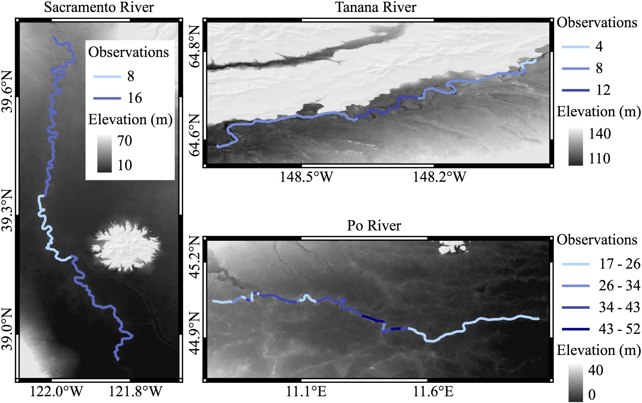
Figure 1. Locations of the three study areas. River centerlines are in blue scale, colored by the number of simulated observations. Grayscale elevations are from the MERIT DEM.

TABLE 1

Table 1. Physical and SWOT simulation characteristics of the sample rivers.

The three river models vary in spatial and temporal extent, and the frequency of simulated SWOT observations varies according to overlap of the planned orbit and the river location. The Po River is the largest set of data in this study, with a full year of simulation, and the Tanana River is the smallest data set, spatially and temporally (Figure 2 and Table 1). Additionally, the smaller node spacing on the Tanana increases noise at the node level, as fewer simulated point measurements are averaged for each node. Similarly, the noise is relatively high for the Sacramento River simulation as it is the narrowest river and fewer simulated observations are available for each node. We removed one high discharge observation from the Sacramento simulation, so that the remaining profiles better represent the average elevation profile. At high discharge, small-scale details of the elevation profile can be lost, or muted, as larger hydraulic controls extend their influence further upstream (Dingman, 2009). Input rasters to the SWOT simulator are sampled in space and time and summarized to nodes matching the simulator output, which allows direct comparisons of the input and output nodes for error analysis of SWOT.

FIGURE 2

Figure 2. Timing of the simulated overpasses for all three rivers. The observations have been aligned such that the first observation of each river is day 1.

DEM Data

We acquired existing DEMs in order to compare the anticipated errors in SWOT river elevation profiles to current elevation data, including SRTM, MERIT, ASTER, NED, ArcticDEM, TanDEM-X, and TINITALY DEMs, where available. For the Sacramento River, we acquired lidar data from the California Valley Floodplain Evaluation and Delineation Program and created a 10 m resolution raster from the last returns (California Department of Water Resources, 2013). We have not included any satellite altimeters in our analysis as the spatial scales of these data are too coarse compared to the other DEMs. We sampled elevations from the DEMs using hand-drawn river centerlines densified to the raster resolution. Manually drawing centerlines for each river ensures elevations are sampled from within the channel, which can change location between data sources. Height errors and missing data in the DEMs caused automated methods of centerline delineation to fail in many cases, due to higher elevations within the channel than outside. Centerlines were manually identified based on changes in data quality over open water and from referencing satellite imagery. The sampled DEM elevations are projected onto average centerlines from the SWOT simulations and transformed to flow distance and cross-channel coordinates (Legleiter and Kyriakidis, 2008). This process allows direct comparison of elevations originally sampled from different centerlines using the common flow distance coordinate. Last, we upscale the DEM profiles to the spacing of the SWOT simulated nodes using a windowed mean and interpolate the DEM data at the flow distance of each simulated node (left side of Figure 3). The end result of this processing is a separate elevation profile from each DEM projected on to a common coordinate system. To analyze the errors, we compare the DEM profiles to the average hydrodynamic model output for all three rivers, as well as boat-mounted GPS profiles of the Sacramento and Tanana Rivers. The GPS data collection is described by Minear and Wright (2016) for the Sacramento River, and by Altenau et al. (2016) for the Tanana River.

FIGURE 3

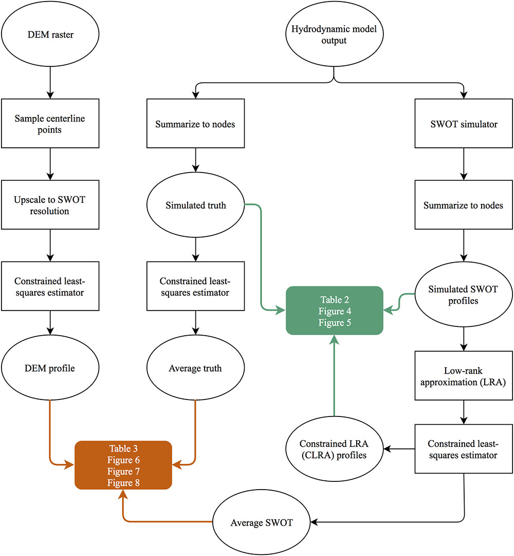
Figure 3. Flow chart of processing and smoothing methods of elevation data. Ovals represent data and rectangles represent processes.

Profile Smoothing

There are many published methods to make noisy DEM surfaces more suitable for hydrologic research, including filling (Jenson and Domingue, 1988), carving (Soille et al., 2003), spline regression (Harbor et al., 2005), and slope-constrained quantile regression (Schwanghart and Scherler, 2017). One reach definition method being considered for SWOT operations uses a Gaussian smoothing filter to reduce noise on SWOT profiles. The Gaussian weighting function used in the filter has two formulations: one uses a static 2 km standard deviation, and the other uses 1/5 of the reach length and a minimum of 1 km standard deviation. Both of these smoothing operations result in very smooth profiles that accurately capture slopes at 10 km scales (Frasson et al., 2017), but the wide window of the filter means small-scale topographic details such as riffle-pool structures are often lost.

We present new methods to reduce noise from multitemporal river elevation profiles that rely on the commonalities between repeated measurements instead of spatial smoothing. To reduce the noise in the simulated elevation profiles, we first decompose the elevation data using the singular value decomposition and analyze the resulting eigenvectors (full description in section Low Rank Approximation). The data is then recreated using fewer eigenvectors, reducing variability between observed profiles, and highlighting the real variability of the profiles. We hypothesize that repeated measurements of river elevation can be closely approximated at lower rank. In other words, the elevation profiles are linearly dependent on one another. The matrix becomes full rank when the simulated SWOT noise is added. To reduce the noise, we eliminate many of the eigenvectors to create a low-rank approximation (LRA) of the simulated data. This LRA is then further constrained using a least-squares estimator such that node elevations decrease in the downstream direction (full description in section Slope Constraint).

Low Rank Approximation

The nodes output by the SWOT simulator are arranged in a matrix such that rows represent nodes along the river centerline, columns represent overpasses, and the values are the simulated elevations. Each simulated SWOT orbit track observes a different set of nodes, which results in an inconsistent number of observations for each node. For example, the middle reaches of the Sacramento river are only observed by half of the simulated overpasses (Figure 1). As a result, the matrix has missing values, and the decomposition does not have a unique solution in this case. To overcome this problem, the river is divided into sections such that all nodes in a given section have the same number of observations (similar to the sections defined by shades of blue in Figure 1). Before the decomposition, we remove the mean simulated elevation of each node, which allows us to analyze the relationship between observations, instead of the overall slope of the river. We decompose the data matrix A into two sets of eigenvectors and corresponding singular values that represent the weight of each vector pair as follows:

$$A=U\ast S\ast V^{\text{T}}(1)$$

Where A is the data matrix, U is a set of eigenvectors that describe relationships between river nodes, V is a set of eigenvectors that describe relationships between overpasses, and S is a diagonal matrix of singular values that relate U and V. The first eigenvector of U represents the most common representation of all the profiles and subsequent eigenvectors describe variations on that profile. The data is recombined from a subset of these eigenvectors:

$$\tilde{A}=U_{\text{k}}\ast S_{\text{k}}\ast V_{\text{k}}^{\text{T}}(2)$$

Where à is the best rank k approximation of A in a least-squares sense, U_k and $V_{\text{k}}^{\text{T}}$ are the first k eigenvectors, and S_k is a diagonal matrix containing the first k singular values (Eckart and Young, 1936).

The LRA is dependent on the number and combination of eigenvectors picked, and the addition of SWOT-like noise to our data makes this decision more difficult. The magnitude of the SWOT noise at this spatial scale means the singular values will not taper off to zero but instead gradually decrease. To identify a cutoff threshold for the singular values, we use parallel analysis (Horn, 1965) followed by a test for significance between orbits in the V matrix. We calculate an average singular value spectrum from 1000 realizations of random, normally distributed data using the sample standard deviation of the simulated SWOT errors. Singular values from the simulated SWOT data that are greater than the corresponding average singular value from the random data are retained.

As a last step in the factor analysis, we test each eigenvector in the V matrix to check if they distinguish between orbit tracks. Different orbits will observe the same river nodes at different ranges of the radar swath, resulting in different error characteristics for each orbit (Fernandez, 2017). The V matrix contains eigenvectors that scale the effect of the U eigenvectors for each overpass. We test each eigenvector in the V matrix to check for statistically significant distributions for each orbit track using a Wilcoxon rank sum test at 95% confidence. We interpret any eigenvector in V that shows different distributions when grouped by orbit as errors related to the viewing angle, and not related to real changes in the water surface. The remaining eigenvectors are interpreted to represent the real variability in the elevation profiles as a result of discharge variability.

Slope Constraint

We also apply a second method of noise reduction: a slope-constrained least-squares estimator, requiring each node elevation to be less than or equal to the upstream node elevation. The constrained profiles are calculated by solving the following equations:

$$minimize\left|\right|G\ast \widehat{z}-z|{|}_2$$

$$suchthat:C\ast \widehat{z}\le b(3)$$

Where z is the observed heights, ẑ is the constrained heights, G is a matrix that relates ẑ and z,b is a vector of zeros to represent the maximum allowable difference between downstream and upstream nodes, and C is a matrix that calculates the difference between nodes when multiplied by ẑx. Solving for ẑx gives the least-squares set of elevations that decrease in the downstream direction.

The formulation of the constrained estimator can produce unwanted results for long sections of observations that display negative slopes. As defined in Equation (3), the solution for these sections has zero slope, and is often followed by a steep slope to compensate (Figure 4). For most rivers, this is not a realistic representation of their slopes and would be problematic for some analyses. We present a modification of Equation (3) to counteract this effect:

FIGURE 4

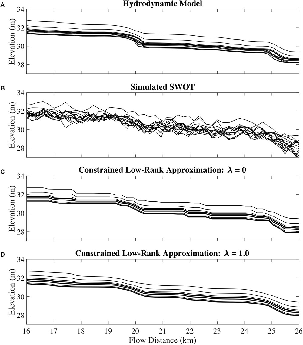
Figure 4. Profile view of a 10 km section of the Sacramento River (A) before and (B) after the simulator noise is added, and (C,D) after the CLRA method is applied. One eigenvector is used in this section.

$$minimize\left|\right|\left[\begin{array}{l}G\\ \lambda \ast C\end{array}\right]\ast \widehat{z}-\left[\frac{z}{d}\right]|{|}_2$$

$$Suchthat:C\ast \widehat{z}\le b(4)$$

Where $\overline{d}$ is the average change in elevation between observed nodes, and λ is a regularization parameter that controls the relative weight of the height and slope terms in the minimization problem. A high λ value penalizes the extreme slopes that can result from Equation (3), whereas a λ value of 0 makes Equations (3) and (4) equivalent. By adding regularization to the estimator, we can come closer to recreating the distribution of slopes we see in the hydrodynamic model (Figure 4D), however, the equation now requires careful parameterization. The example in Figure 4D was parameterized using our knowledge of the true profiles, and as such is optimistic. Using a λ value that is too low has little effect and using one that is too high results in an overly smooth profile with few details. This is the same problem encountered with other smoothing and local regression techniques: the user is forced to pick the smoothness of the resulting profile. The advantage of Equation (3) over these techniques is there is no decision to be made about smoothness, or assumption of the variability of slopes. The height errors are reduced only by the physical constraint that water flows downhill. As such, we use the output of Equation (3) for the remainder of our analysis.

We use the constrained least-squares estimator from Equation (3) in two ways: to constrain the slope of individual profiles and to estimate an average profile from many observations (Figure 3). For our error analysis of the multitemporal simulated SWOT profiles, the constrained least-squares estimator is solved for each overpass separately. These profiles are referred to as the Constrained LRA (CLRA) profiles. We also use the estimator to create an average profile by including all simulated observations in the vector z, and create G to relate all observations at one node to one predicted height in x. This creates one constrained profile from all observations, which we term the average SWOT profile. Combining elevation profiles from different days, which represent a range of discharges, is not a perfect solution to reducing noise, as elevations at different nodes will respond differently to variations in discharge. However, considering the large vertical errors in the raw data, the error introduced at this step are likely comparatively small.

Results

The application of the CLRA method to our simulated SWOT data sets decreased the mean absolute error (MAE) of every simulated profile when compared to the raw SWOT node elevations (Figure 5). Analyzing the errors at an intermediate step shows that both the low rank approximation and the slope constraint result in decreased height errors. Node-scale MAEs were reduced by more than half for all three rivers (Table 2). The Sacramento River showed the largest decrease in MAE, at more than 70% reduction. RMSEs of the node heights show similar improvement. The LRA component of the method reduces error variability between days, which is apparent in Figure 5 as less spread among the days for each river on the vertical axis compared to the horizontal axis.

FIGURE 5

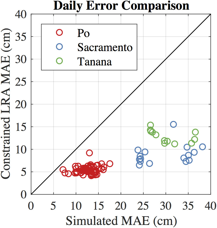
Figure 5. MAE before and after the CLRA method for each observed profile. Points below the 1:1 line indicate the CLRA method decreased the height errors.

TABLE 2

Table 2. Error statistics before and after the CLRA method.

Decomposing the hydrodynamic model output shows us that the first eigenvector from noise-free data always contains more than 95% of the variance in the data for all three rivers, and that the first four eigenvectors always contain more than 99% of the variance. Our factor analysis method for simulated SWOT data resulted in just one eigenvector being used to recreate the data for all locations. Parallel analysis occasionally indicated two eigenvectors should be used to approximate the data, but the test for significant difference between orbits eliminated the second eigenvector in every case.

We applied the constrained least-squares estimator to all the DEM profiles in Figure 6 and for evaluation in Table 3, which reduced errors in all cases. We calculate MAE and RMSE statistics for the DEM-derived and average SWOT profiles for all three rivers compared to the average hydrodynamic model elevation profiles, and for Sacramento and Tanana Rivers compared to the GPS profiles. Comparisons with the hydrodynamic model favor the SWOT simulation, as any inaccuracies in the hydrodynamic model will not affect the SWOT error estimates but will increase errors for the DEMs. Comparisons to the GPS profiles increase errors of the SWOT simulation profiles due to inaccuracies in the hydrodynamic models. Even though there is no fully fair direct comparison, we can see the difference between SWOT and existing DEMs is quite large (Figure 6). The ASTER-derived profiles are relatively coarse, despite the improvements from the constrained least squares estimator. Estimating river surface slopes from these ASTER profiles would require very large reaches. The difference between SRTM and MERIT is small for the Sacramento and Po Rivers, which is to be expected as MERIT is derived from SRTM data in these areas (Yamazaki et al., 2017). The error removal methods used to create MERIT offer some improvement over SRTM for the Sacramento River, but errors are still quite large compared to the SWOT and lidar profile.

FIGURE 6

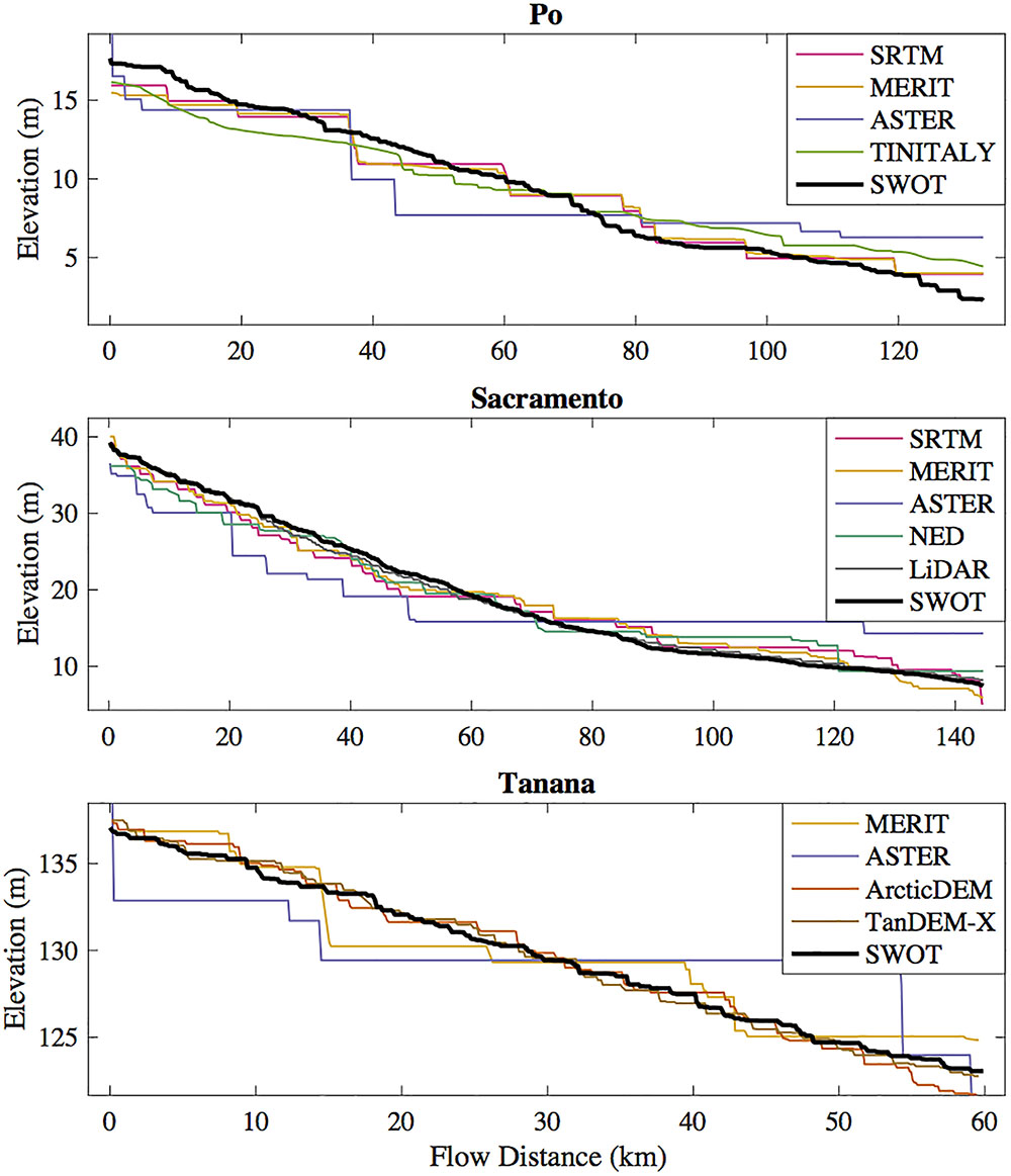
Figure 6. River profiles extracted from existing publicly available DEMs and the simulated SWOT-derived river profiles.

TABLE 3

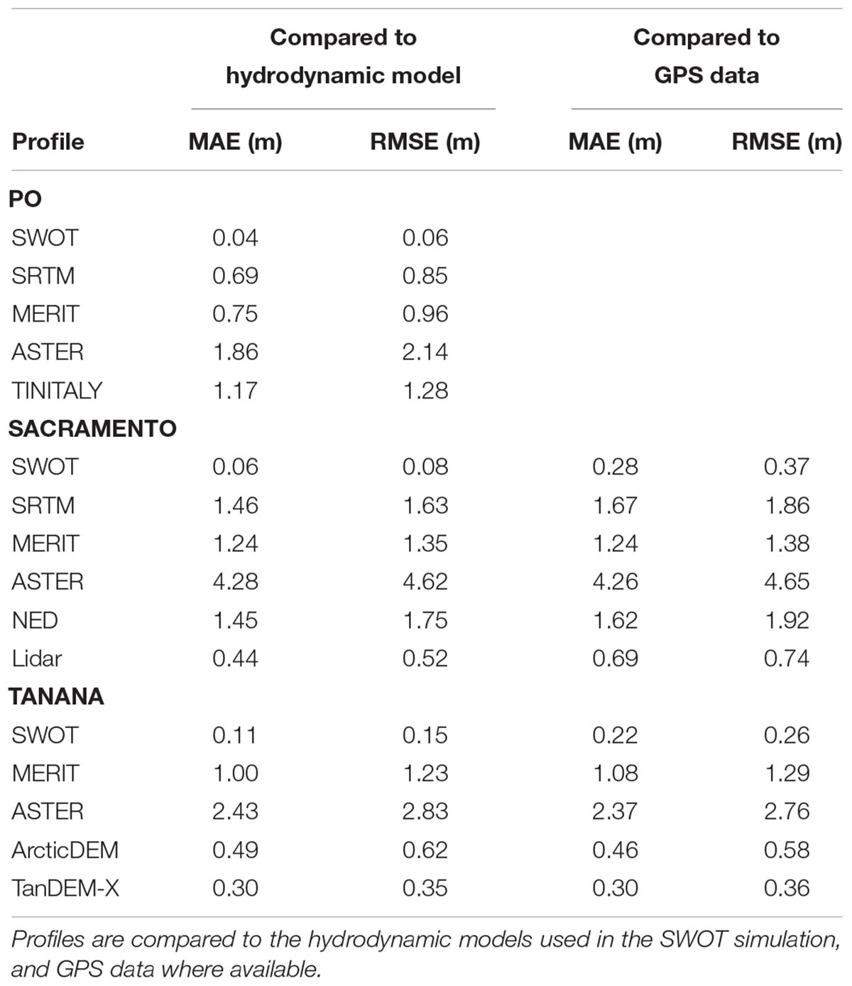
Table 3. Error statistic comparison of simulated SWOT profiles and profiles extracted from existing DEMs.

Applications

Physical Habitats

Riffle-pool sequences in rivers represent distinct physical habitats that also vary ecologically with different invertebrate community composition, density, and biomass (Brown and Brussock, 1991). Yang (1971) defined riffles and pools according to their energy gradient, which can be approximated by the water surface slope, but others have based classifications on channel slope, as it is independent of discharge (Richards, 1976). In practice, classifications of riffle and pool habitats are often subjective, but quantitative analysis of these classifications shows a threshold on surface slope can identify riffles and pools with accuracies of 70 and 79%, respectively (Jowett, 1993). We evaluate the ability of SWOT to find locally steep sections of rivers in comparison to existing elevation data.

We use relative steepness, originally used to identify knickpoints, to identify sections of the simulated Sacramento profiles that are potential riffles or runs. We selected the Sacramento for this application because the upstream reaches show cyclical low-high slope sections (e.g., Figure 4). We use the relative steepness metric in place of a threshold on slope, which would vary between rivers. Relative steepness is defined as the trend in surface slope with increasing reach lengths (Hayakawa and Oguchi, 2006). We use reach lengths from 400 to 20,000 m. High values of relative steepness indicate places where the local slope is very different from the slope over greater lengths; values near zero indicate little change in slope over the range of reach lengths. Similar to Hayakawa and Oguchi (2006), we use a threshold of one standard deviation greater than the mean relative steepness value to classify steep sections. We compare locations where relative steepness exceeds our threshold for the average SWOT and DEM profiles compared to the hydrodynamic model output.

Applying the relative steepness metric to both the hydrodynamic model and the average SWOT profile, we see that we can correctly identify many sub-kilometer high-slope sections of the Sacramento River (Figure 7). The hydrodynamic model for the Sacramento has an average cross sectional spacing of 258 m, so we are confident the 200 m spacing of the elevation nodes will accurately represent the river morphology. A comparison of the GPS and hydrodynamic model profiles confirms the model’s accuracy (mean absolute difference: 13 cm). As such, we evaluate the steepness of the DEMs by comparing them to the hydrodynamic model. Of the 99 nodes we classified as steep in the modeled profiles, we correctly identified 74 nodes in the average SWOT profile. Twenty-five nodes were missed in the classification of the average SWOT profile, and 18 were incorrectly classified as steep. Generally, we identify all of the steep sections of the river, despite having false negatives and positives on the edges of the sections. Near 65 and 115 km flow distance we have false positives far from a true steep point, but the relative steepness of the true profile is near the threshold (Figure 7). We also perform this test on the water surface DEM profiles of the Sacramento River and calculate standard positive predictive values, false negative rates, and false positive rates (Table 4). The results of the steepness classification for the DEMs mirror the height error results in Table 3. SWOT outperforms the existing DEMs in all three metrics. SRTM, MERIT, and NED perform similarly, correctly identifying 20, 16, and 17 nodes. lidar captures the steep sections best of the existing DEMs, correctly identifying 42 nodes.

FIGURE 7

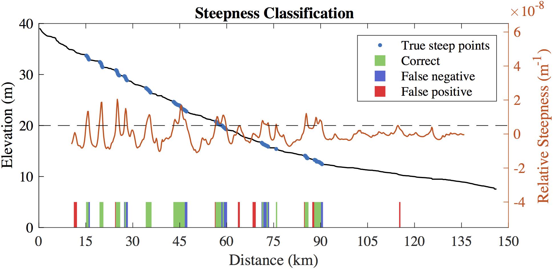
Figure 7. Average truth profile for the Sacramento River with calculated relative steepness values and threshold (black dashed line). The colored bars on the bottom compare the classification of the average truth and SWOT profiles.

TABLE 4

Table 4. Classification statistics for the relative steepness threshold.

The relative steepness metric we use on the Sacramento River shows us that we can find the local steep sections of rivers despite the level of noise anticipated from SWOT. While slope is not a perfect predictor of physical habitat, it is a good indicator as shown by Jowett (1993). More sophisticated habitat models could be used as well, such as the in-stream habitat classification models from Demarchi et al. (2016) that use lidar and multispectral imagery. The centimeter-scale errors we report for average SWOT profiles suggest SWOT could be used as a coarse-resolution alternative to lidar for similar models, with the advantage that it will be available over nearly the entire globe.

Tectonics

Fault movements and the growth of associated folds can disrupt a river network in equilibrium, as rivers are sensitive to topographic changes. Large displacements can cause rerouting of river networks, whereas small displacements may result in changes to hydraulic geometry variables such as channel concavity, meander wavelength, and floodplain width as the river adjusts to external topographic gradients imposed by a regional tectonic deformation field in an effort to maintain, or reestablish an equilibrium longitudinal profile (Schumm, 1986). In large alluvial rivers that flow over areas of known tectonic activity, we hypothesize that SWOT will be able to observe anomalies in the elevation profile of rivers potentially related to buried fault and fold structures that are unobservable in existing DEMs.

We test our hypothesis by examining the concavity of the average SWOT elevation profile for the Po River, located in northern Italy between the Apennines and southern Alps, as an example of a low-relief fluvial plain (Po Plain) with no obvious topographic expression of active tectonics, where such a signal may be recorded in spatial variations in channel elevations. The Po River flows eastward along the axis of the foreland basin formed in front of the northward propagating Apennine accretionary wedge (Castellarin, 2001). At the latitude of the river, the frontal portion of the Apennine fold and thrust belt, referred to as the Ferrara-Romagna arc in the eastern Po Plain, is buried by several kilometers of Quaternary clastic sediment and there are no obvious surface topographic expressions of the underlying faults or folds; although the structures are well-imaged by seismic refraction studies and have been intersected in hydrocarbon exploration wells (e.g., Bigi et al., 1992). The buried frontal portion of the Apennine accretionary wedge is seismically active, as exemplified by two damaging earthquakes in May of 2012, a Mw 6.1 followed 9 days later by a Mw 5.8, that were sourced on blind, shallow (<10 km) thrust faults of the Ferrara arc that project north and up-dip toward the Po River (Burrato et al., 2012).

Previous investigators have identified and interpreted plan-view anomalies in drainage patterns of the Po and its tributaries as evidence for the subtle perturbation of surface topography above blind thrust faults (Burrato et al., 2003), like the ones responsible for the deadly 2012 earthquakes (Burrato et al., 2012). In our analysis of the elevation of the Po River channel we first smooth the average SWOT profile using a 10 km wide windowed mean filter, and then calculate the second derivative of the elevation profile over 20 km. We find there is a spatial coincidence between the concavity of the average SWOT elevation profile of the Po River and the underlying structural geology. The highest calculated longitudinal profile concavity and convexity (negative concavity) values along the study reach are centered around 80 and 65 km flow distance, respectively. Both of these profile inflections coincide with the intersection of the river and the outermost buried thrust faults of the Ferrara arc portion of the Apennine accretionary wedge (Figure 8). Away from the Ferrara arc faults, the river profile shows less extreme concavity values.

FIGURE 8

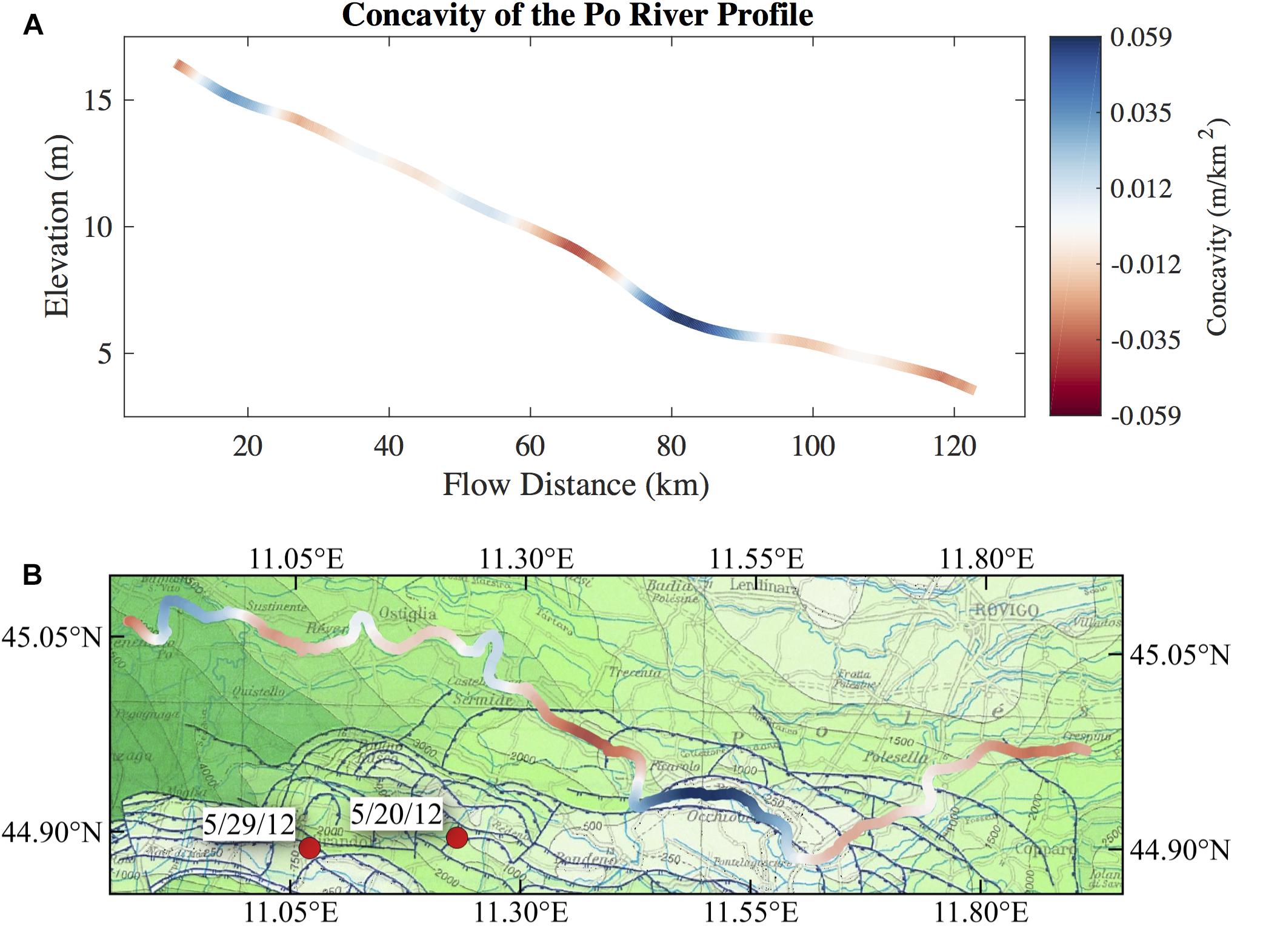
Figure 8. (A) Smoothed average SWOT profile of the Po River colored by curvature. The elevation profile was smoothed using a 10 km mean window, and curvature calculated using a 20 km window. (B) Po River centerline plotted on top of the structural geology of the Po Plain (http://portalesgi.isprambiente.it/) with the same concavity color scale from (A). The epicenters of two large earthquakes in 2012 are plotted in red.

Mapping the concavity of the Po River profile, calculated from SWOT simulations, on top of the structural geology of the Po Plain suggests that SWOT data can be a useful tool in tectonic geomorphology. The high concavity section of the Po in Figure 8 is spatially coincident with an anomalous reach (anomaly #19) identified by Burrato et al. (2003) as evidence for active blind thrust faulting beneath this portion of the Po Plain. Burrato et al. (2003) did not find any other anomalies in our simulated section of the Po, consistent with our interpretation of the SWOT-derived concavity values. Figure 9 shows the concavity of the available DEMs in addition to the hydrodynamic model and the average SWOT profile for the Po River. Existing DEMs show much higher concavity values than the hydrodynamic model, and with no signature of the anomalous reach identified in the average SWOT profile at a flow distance of 80 km (Figure 8) and in Burrato et al. (2003). Looking at Figure 6, the absence of a convincing concavity signature in the DEM profiles is not surprising. The vertical error in the DEMs, even at scales of tens of kilometers, obscures the effects of tectonics on the elevation profile of the Po River. Ultimately, our conclusions are based on the hydrodynamic model of the Po, but through the lens of the SWOT simulator. The features we are evaluating in this application are on the scale of tens of kilometers, so we expect the bathymetric cross section spacing of 1.2 km to accurately capture these features. The hydrodynamic model was corrupted and subsampled by the SWOT simulator in order to evaluate the potential for SWOT to see the same curvature features. Our simulated Po River profile suggests that SWOT will be able to resolve anomalous curvatures in similar rivers around the world where existing DEMs cannot.

FIGURE 9

Figure 9. Calculated concavity for all water surface profiles of the Po River.

Conclusion

The CLRA method presented here greatly improves the node-level errors of river elevation profiles from SWOT by taking advantage of repeated measurements. The singular value decomposition allows us to reduce variation between profiles, largely caused by noise, while retaining some of the real variation in slope due to partial controls. Partial controls are channel features that have less effect on the surface slope with increasing discharge (Dingman, 2009). The results presented in Figure 4 demonstrate that the CLRA profiles are able to capture changes in slope with changing stage. The elevation drop around 20 km flow distance in Figure 4 is less pronounced when the river is at high stage, which is observable in both the simulated truth and the final CLRA profiles.

The Po River has the lowest error of all three rivers analyzed, both before and after the CLRA method. We believe the relatively low error in the simulated SWOT profiles is due to the Po being the widest river in our study, which means more simulated measurements are averaged for each node along the river centerline. While the final MAE is the lowest for the Po, the reduction in MAE by the CLRA method is greatest for the Sacramento at 70.45%. We would expect the 52 simulated overpasses of the Po to make the LRA component of the methods more effective than on the Tanana, where only 12 overpasses were simulated, but the change in MAE is approximately the same. It is reasonable to assume that some rivers can be represented with fewer eigenvectors than other rivers, but it is currently unclear what characteristics of the river, or of the SWOT noise, controls performance of the CLRA method. Future application to additional rivers will improve understanding of the algorithm performance.

SWOT is anticipated to provide WSE measurements more accurate than existing publicly available data. lidar data can provide high-resolution, high-accuracy elevation measurements over water surfaces, but is not available in most areas. Where lidar is available, it is often only at one point in time, which limits the study of many dynamic riverine processes. In comparison, SWOT will observe rivers wider than 50–100 m between 78° north and south an average of twice per 21 days, or about 35 times per year (Biancamaria et al., 2016). We show that an average of SWOT observations will have accuracies better than available DEMs scaled to 100–200 m along-stream resolution. The development of a new CLRA method reduces errors in the multitemporal river profiles, without sacrificing spatial resolution like many smoothing algorithms. Creating an average SWOT profile reduces the errors even further and provides a static profile that can be used in a similar manner to existing DEMs. We show the ability of average SWOT profiles to capture changes in slope, for example, that are ecologically important for the identification of physical habitat variability for aquatic organisms. We also demonstrate that changes in river curvature identifiable in averaged SWOT profiles, may provide evidence for the subtle deformation of the Earth’s surface by buried thrust faults beneath an alluvial plain, promising to provide geomorphologists a new dataset from which to decipher active tectonics.

Author Contributions

TL and TP analyzed the data and wrote the manuscript. EA created the Tanana River hydrodynamic model and provided SWOT simulation data. AD created the Po River hydrodynamic model. RW and RF provided the SWOT simulation data of the Sacramento and Po Rivers. MD helped to develop the methods. MF advised on the physical habitats section. KW contributed to the tectonics section. All authors reviewed the final manuscript.

Funding

This research was funded by Subcontract #1553389 from the SWOT Project Office at the NASA/Caltech Jet Propulsion Lab.

Disclaimer

This work is not a product of the U.S. Government or the U.S. Environmental Protection Agency, and the author/editor/speaker is not doing this work in any governmental capacity. The views expressed are those of the authors only and do not necessarily represent those of the U.S. Government or the EPA. The findings and conclusions in this report have not been formally disseminated by the U.S. EPA and should not be construed to represent any agency determination or policy.

Conflict of Interest Statement

The authors declare that the research was conducted in the absence of any commercial or financial relationships that could be construed as a potential conflict of interest.

Acknowledgments

We thank JN and KA for their input and help improving the manuscript.

Footnote

1. ^http://arcticdem.org

References

Alsdorf, D. E., Rodriguez, E., and Lettenmaier, D. P. (2007). Measuring surface water from space. Rev. Geophys. 45, 1–24. doi: 10.1029/2006RG000197

CrossRef Full Text | Google Scholar

Altenau, E. H., Pavelsky, T. M., Bates, P. D., and Neal, J. C. (2017). The effects of spatial resolution and dimensionality on modeling regional-scale hydraulics in a multichannel river. Water Resour. Res. 53, 1683–1701. doi: 10.1002/2016WR019396

CrossRef Full Text | Google Scholar

Altenau, E. H., Pavelsky, T. M., Moller, D., Lion, C., Pitcher, L. H., Allen, G. H., et al. (2016). AirSWOT measurements of river water surface elevation and slope: Tanana River, AK. Geophys. Res. Lett. 44, 181–189. doi: 10.1002/2016GL071577

CrossRef Full Text | Google Scholar

Biancamaria, S., Lettenmaier, D. P., and Pavelsky, T. M. (2016). The SWOT mission and its capabilities for land hydrology. Surv. Geophys. 37, 307–337. doi: 10.1007/s10712-015-9346-y

CrossRef Full Text | Google Scholar

Bigi, G., Cosentino, D., Parotto, M., Sartori, R., and Scandone, P. (1992). Structural model of Italy and Gravity Map 1:500,000. Roma: Monografie Progetto Finalizzato Geodinamica, CNA.

Google Scholar

Birkett, C. M., Mertes, L. A. K., Dunne, T., Costa, M. H., and Jasinski, M. J. (2002). Surface water dynamics in the amazon basin: application of satellite radar altimetry. J. Geophys. Res. Atmos. 107, LBA 26-1–LBA 26-21. doi: 10.1029/2001JD000609

CrossRef Full Text | Google Scholar

Biron, P. M., Choné, G., Buffin-Bélanger, T., Demers, S., and Olsen, T. (2013). Improvement of streams hydro-geomorphological assessment using LiDAR DEMs. Earth Surf. Process. Landforms 38, 1808–1821. doi: 10.1002/esp.3425

CrossRef Full Text | Google Scholar

Brown, A. V., and Brussock, P. P. (1991). Comparisons of benthic invertebrates between riffles and pools. Hydrobiologia 220, 99–108.

Google Scholar

Burrato, P., Ciucci, F., and Valensise, G. (2003). An inventory of river anomalies in the po plain, Northern Italy: evidence for active blind thrust faulting. Ann. Geophys. 46, 1–18.

Google Scholar

Burrato, P., Vannoli, P., Fracassi, U., Basili, R., and Valensise, G. (2012). Is blind faulting truly invisible? Tectonic-controlled drainage evolution in the epicentral area of the May 2012, Emilia-Romagna earthquake sequence (northern Italy). Ann. Geophys. 55, 525–531. doi: 10.4401/ag-6182

CrossRef Full Text | Google Scholar

California Department of Water Resources (2013). Lidar data collection for the CVFED Floodsafe Initiative, Sacramento and San Joaquin Rivers and surrounding areas. Available at: https://water.ca.gov/Programs/Flood-Management

Google Scholar

Castellarin, A. (2001). “Alps-apennines and po plain-frontal apennines relations,” in Anatomy of an Orogen: The Apennines and Adjacent Mediterranean Basins, eds G. B. Vai and I. P. Martini (Dordrecht: Kluwer Academic Publishers), 177–196.

Google Scholar

Castellarin, A., Domeneghetti, A., and Brath, A. (2011). Identifying robust large-scale flood risk mitigation strategies: a quasi-2D hydraulic model as a tool for the Po river. Phys. Chem. Earth 36, 299–308. doi: 10.1016/j.pce.2011.02.008

CrossRef Full Text | Google Scholar

Dai, C., Durand, M., Howat, I. M., Altenau, E. H., and Pavelsky, T. M. (2018). Estimating river surface elevation from ArcticDEM. Geophys. Res. Lett. 45, 3107–3114. doi: 10.1002/2018GL077379

CrossRef Full Text | Google Scholar

Demarchi, L., Bizzi, S., and Piégay, H. (2016). Hierarchical object-based mapping of riverscape units and in-stream mesohabitats using LiDAR and VHR imagery. Remote Sens. 8:97. doi: 10.3390/rs8020097

CrossRef Full Text | Google Scholar

Dias, M. S., Cornu, J. F., Oberdorff, T., Lasso, C. A., and Tedesco, P. A. (2013). Natural fragmentation in river networks as a driver of speciation for freshwater fishes. Ecography 36, 683–689. doi: 10.1111/j.1600-0587.2012.07724.x

CrossRef Full Text | Google Scholar

Dingman, S. L. (2009). Fluvial Hydraulics. Oxford: Oxford University Press.

Google Scholar

Domeneghetti, A., Schumann, G. J.-P., Frasson, R. P. M., Wei, R., Pavelsky, T. M., Castellarin, A., et al. (2018). Characterizing water surface elevation under different flow conditions for the upcoming SWOT mission. J. Hydrol. 561, 848–861. doi: 10.1016/J.JHYDROL.2018.04.046

CrossRef Full Text | Google Scholar

Eckart, C., and Young, G. (1936). The approximation of one matrix by another of lower rank. Psychometrika 1, 211–218. doi: 10.1007/BF02288367

CrossRef Full Text | Google Scholar

Fernandez, D. E. (2017). SWOT Mission Performance and Error Budget. Pasadena, CA: Jet Propulsion Laboratory.

Google Scholar

Frasson, R. P. D. M., Wei, R., Durand, M., Minear, J. T., Domeneghetti, A., Schumann, G., et al. (2017). Automated river reach definition strategies: applications for the surface water and ocean topography mission. Water Resour. Res. 53, 8164–8186. doi: 10.1002/2017WR020887

CrossRef Full Text | Google Scholar

Gesch, D., Oimoen, M., Greenlee, S., Nelson, C., Steuck, M., and Tyler, D. (2002). The national elevation dataset. Photogramm. Eng. Remote Sens. 68, 5–11.

Google Scholar

Hannah, D. M., Demuth, S., van Lanen, H. A. J., Looser, U., Prudhomme, C., Rees, G., et al. (2011). Large-scale river flow archives: importance, current status and future needs. Hydrol. Process. 25, 1191–1200. doi: 10.1002/hyp.7794

CrossRef Full Text | Google Scholar

Harbor, D., Bacastow, A., Heath, A., and Rogers, J. (2005). Capturing variable knickpoint retreat in the central appalachians. U.S.A. Geogr. Fis. E Din. Quat. 28, 23–36.

Google Scholar

Hayakawa, Y. S., and Oguchi, T. (2006). DEM-based identification of fluvial knickzones and its application to Japanese mountain rivers. Geomorphology 78, 90–106. doi: 10.1016/J.GEOMORPH.2006.01.018

CrossRef Full Text | Google Scholar

Horn, J. L. (1965). A rationale and test for the number of factors in factor analysis. Psychometrika 30, 179–185. doi: 10.1007/BF02289447

CrossRef Full Text | Google Scholar

Jenson, S. K., and Domingue, J. O. (1988). Extracting topographic structure from digital elevation data for geographic information system analysis. Photogramm. Eng. Remote Sens. 54, 1–8.

Google Scholar

Jowett, I. G. (1993). A method for objectively identifying pool, run, and riffle habitats from physical measurements. New Zeal. J. Mar. Freshw. Res. 27, 241–248. doi: 10.1080/00288330.1993.9516563

CrossRef Full Text | Google Scholar

Koblinsky, C. J., Clarke, R. T., Brenner, A. C., and Frey, H. (1993). Measurement of river level variations with satellite altimetry. Water Resour. Res. 29, 1839–1848. doi: 10.1029/93WR00542

CrossRef Full Text | Google Scholar

LeFavour, G., and Alsdorf, D. (2005). Water slope and discharge in the Amazon River estimated using the shuttle radar topography mission digital elevation model. Geophys. Res. Lett. 32:L17404. doi: 10.1029/2005GL023836

CrossRef Full Text | Google Scholar

Legleiter, C. J., and Kyriakidis, P. C. (2008). Spatial prediction of river channel topography by kriging. Earth Surf. Process. Landforms 33, 841–867. doi: 10.1002/esp.1579

CrossRef Full Text | Google Scholar

Minear, J. T., and Wright, S. (2016). Water-Surface Elevations and Temperature Data Collected for the NASA/JPL AirSWOT Campaign on the Sacramento River, Near Colusa, CA, for the Period March – May, 2015. Reston, VA: U.S. Geological Survey.

Google Scholar

Papa, F., Bala, S. K., Pandey, R. K., Durand, F., Gopalakrishna, V. V., Rahman, A., et al. (2012). Ganga-Brahmaputra river discharge from Jason-2 radar altimetry: an update to the long-term satellite-derived estimates of continental freshwater forcing flux into the Bay of Bengal. J. Geophys. Res. 117, 1–13. doi: 10.1029/2012jc008158

CrossRef Full Text | Google Scholar

Richards, K. S. (1976). The morphology of riffle-pool sequences. Earth Surf. Process. 1, 71–88. doi: 10.1002/esp.3290010108

CrossRef Full Text | Google Scholar

Schumann, G. J. P., and Domeneghetti, A. (2016). Exploiting the proliferation of current and future satellite observations of rivers. Hydrol. Process. 30, 2891–2896. doi: 10.1002/hyp.10825

CrossRef Full Text | Google Scholar

Schumm, S. A. (1986). “Alluvial river response to active tectonics,” in Active Tectonics: Impact on Society, ed. National Research Council (Washington, DC: National Academy Press), 80–82.

Google Scholar

Schwanghart, W., and Scherler, D. (2017). Bumps in river profiles: uncertainty assessment and smoothing using quantile regression techniques. Earth Surf. Dynam 55194, 821–839. doi: 10.5194/esurf-5-821-2017

CrossRef Full Text | Google Scholar

Shiklomanov, A. I., Lammers, R. B., and Vörösmarty, C. J. (2002). Widespread Decline in Hydrological Monitoring Threatens Pan-Arctic Research. Washington, DC: EOS.

Google Scholar

Soille, P., Vogt, J., and Colombo, R. (2003). Carving and adaptive drainage enforcement of grid digital elevation models. Water Resour. Res. 39, 1366–1378. doi: 10.1029/2002WR001879

CrossRef Full Text | Google Scholar

Tachikawa, T., Hat, M., Kaku, M., and Iwasaki, A. (2011). “Characteristics of aster gdem version 2 1 earth remote sensing data analysis center (ERSDAC), 2 mitsubishi material techno corp. 3 University of Tokyo,” in Proceedings of the Geoscience Remote Sensing Symposium (IGARSS), (Vancouver, BC), 3657–3660.

Google Scholar

Tarquini, S., Vinci, S., Favalli, M., Doumaz, F., Fornaciai, A., and Nannipieri, L. (2011). Release of a 10-m-resolution DEM for the Italian territory: comparison with global-coverage DEMs and anaglyph-mode exploration via the web. Comput. Geosci. 38, 168–170. doi: 10.1016/j.cageo.2011.04.018

CrossRef Full Text | Google Scholar

Wendleder, A., Wessel, B., Roth, A., Breunig, M., Martin, K., and Wagenbrenner, S. (2013). TanDEM-X water indication mask: generation and first evaluation results. IEEE J. Sel. Top. Appl. Earth Obs. Remote Sens. 6, 171–179. doi: 10.1109/JSTARS.2012.2210999

CrossRef Full Text | Google Scholar

Whipple, K. X., and Tucker, G. E. (1999). Dynamics of the stream-power river incision model: implications for height limits of mountain ranges, landscape response timescales, and research needs. J. Geophys. Res. Solid Earth 104, 17661–17674. doi: 10.1029/1999JB900120

CrossRef Full Text | Google Scholar

Yamazaki, D., Ikeshima, D., Tawatari, R., Yamaguchi, T., O ’loughlin, F., Neal, J. C., et al. (2017). A high-accuracy map of global terrain elevations. Geophys. Res. Lett. 44, 5844–5853. doi: 10.1002/2017GL072874

CrossRef Full Text | Google Scholar

Yang, C. T. (1971). Formation of rilfles and pools. Water Resour. Res. 7, 1567–1574. doi: 10.1029/WR007i006p01567

PubMed Abstract | CrossRef Full Text | Google Scholar