
95% of researchers rate our articles as excellent or good
Learn more about the work of our research integrity team to safeguard the quality of each article we publish.
Find out more
ORIGINAL RESEARCH article
Front. Earth Sci. , 18 June 2019
Sec. Atmospheric Science
Volume 7 - 2019 | https://doi.org/10.3389/feart.2019.00100
This article is part of the Research Topic From the Satellite to the Earth's Surface: Studies Relevant to NASA’s Plankton, Aerosol, Cloud, Ocean Ecosystems (PACE) Mission View all 10 articles
 Jacek Chowdhary1*†
 Peng-Wang Zhai2†
 Emmanuel Boss3
 Heidi Dierssen4
 Robert Frouin5
 Amir Ibrahim6
 Zhongping Lee7
 Lorraine A. Remer8
 Michael Twardowski9
 Feng Xu10Xiaodong Zhang11,12
 Matteo Ottaviani13
 William Reed Espinosa14
 Didier Ramon15
The research frontiers of radiative transfer (RT) in coupled atmosphere-ocean systems are explored to enable new science and specifically to support the upcoming Plankton, Aerosol, Cloud ocean Ecosystem (PACE) satellite mission. Given (i) the multitude of atmospheric and oceanic constituents at any given moment that each exhibits a large variety of physical and chemical properties and (ii) the diversity of light-matter interactions (scattering, absorption, and emission), tackling all outstanding RT aspects related to interpreting and/or simulating light reflected by atmosphere-ocean systems becomes impossible. Instead, we focus on both theoretical and experimental studies of RT topics important to the science threshold and goal questions of the PACE mission and the measurement capabilities of its instruments. We differentiate between (a) forward (FWD) RT studies that focus mainly on sensitivity to influencing variables and/or simulating data sets, and (b) inverse (INV) RT studies that also involve the retrieval of atmosphere and ocean parameters. Our topics cover (1) the ocean (i.e., water body): absorption and elastic/inelastic scattering by pure water (FWD RT) and models for scattering and absorption by particulates (FWD RT and INV RT); (2) the air-water interface: variations in ocean surface refractive index (INV RT) and in whitecap reflectance (INV RT); (3) the atmosphere: polarimetric and/or hyperspectral remote sensing of aerosols (INV RT) and of gases (FWD RT); and (4) atmosphere-ocean systems: benchmark comparisons, impact of the Earth’s sphericity and adjacency effects on space-borne observations, and scattering in the ultraviolet regime (FWD RT). We provide for each topic a summary of past relevant (heritage) work, followed by a discussion (for unresolved questions) and RT updates.
Plankton, Aerosol, Cloud ocean Ecosystem (PACE; see Table 1 for a list of all acronyms used in this manuscript) is NASA’s Plankton, Aerosol, Cloud, ocean Ecosystem mission1, currently in the formulation phase of mission development. It is scheduled for launch in 2022 into a Sun synchronous, 676.5-km-high polar orbit with an inclination of 98° and a local equatorial crossing time of 1 pm. The science goals for this mission are (NASA, 2018a): (1) to extend past and current key systematic ocean color, aerosol, and cloud data records for Earth system and climate studies; and (2) to address new and emerging oceanic and atmospheric science questions using advanced instruments. To provide the requisite data for these goals, the PACE platform will carry three satellite instruments: the Ocean Color Instrument (OCI), the Spectro-Polarimeter for Planetary Exploration (SPEXone) (Hasekamp et al., 2019), and the Hyper Angular Rainbow Polarimeter (HARP2) (Martins et al., 2014). Together, these instruments will be the most advanced in NASA’s history for the combined observation of ocean color and atmospheric aerosols, and will therefore provide unprecedented research opportunities. At the same time, the advanced remote sensing capabilities that these instruments offer places also require stringent requirements for forward and inverse radiative transfer (RT) modeling of light reflected by atmosphere-ocean systems. Before describing the status and various updates for such RT modeling, we summarize the measurement capabilities of OCI, SPEXone and HARP2 for PACE.
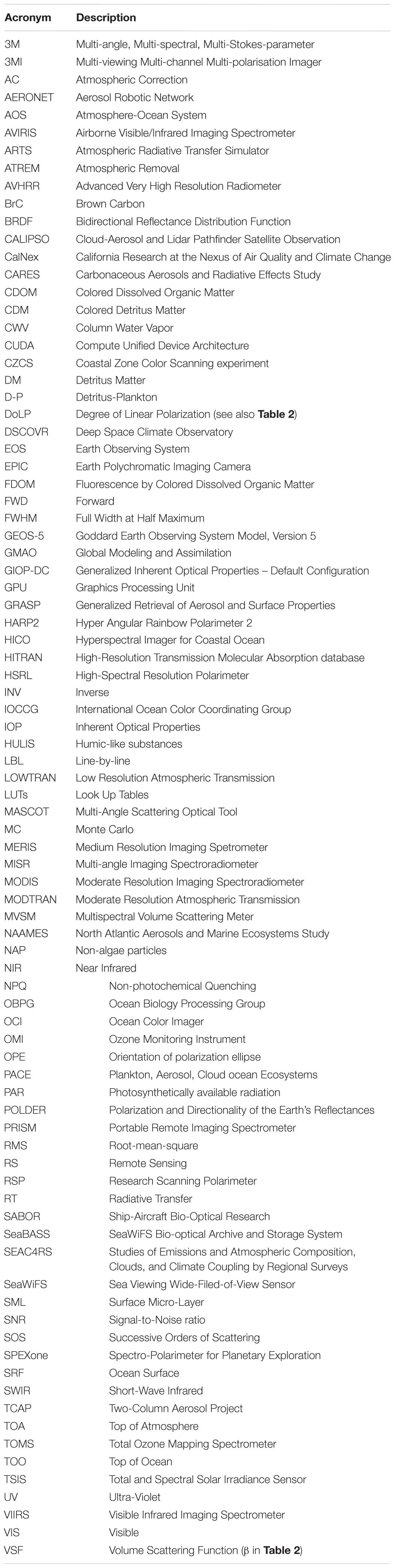
Table 1. List of acronyms.
The width of an OCI image will be 2,663 km (which leads to a two-day ocean color coverage of the globe), and the spatial resolution will be 1 km for nadir viewing pixels. OCI will make single-view, hyperspectral radiance measurements for each pixel at a spectral resolution of 5 nm that cover the ultraviolet (UV) regime between 350 and 400 nm, the visible (VIS) between 400 and 700 nm, and the near infrared (NIR) regime between 700 and 885 nm. In addition, OCI will obtain single-view, narrow-band radiance measurements for each pixel in the short-wave infrared (SWIR) regime at nine wavelengths (940, 1038, 1250, 1378, 1615, 2130, and 2260 nm). The signal-to-noise ratio (SNR) for a typical ocean scene will be 1000 and 600 for the hyperspectral measurements in the UV-VIS and NIR regimes, respectively. These SNR values adhere to one of the threshold measurement requirements for PACE (NASA, 2018a), which is to retrieve the water-leaving radiance (that typically contributes less than 10% to space-borne radiance) with an accuracy in the VIS of the maximum of either 5%, or 0.002 for water reflectance ρw (see Table 2 for definition and unit of all parameters used in this manuscript). Due to the high degree of empiricism present in retrieval algorithms of ocean inherent optical properties (IOP), the accuracy requirements for IOP retrievals are not defined for PACE. However, it is well established that the addition of bands and increase in SNR when compared to past ocean color missions should improve the retrievals relative to the current state of the art. The ultimate evaluation the IOP retrieval performance will take place by comparing with co-located independent IOP measurement sets. More information on the measurement requirements for OCI, as well as the threshold and goal science questions targeted by these measurements, can be found in the Science Definition Report prepared for PACE (NASA, 2018a).
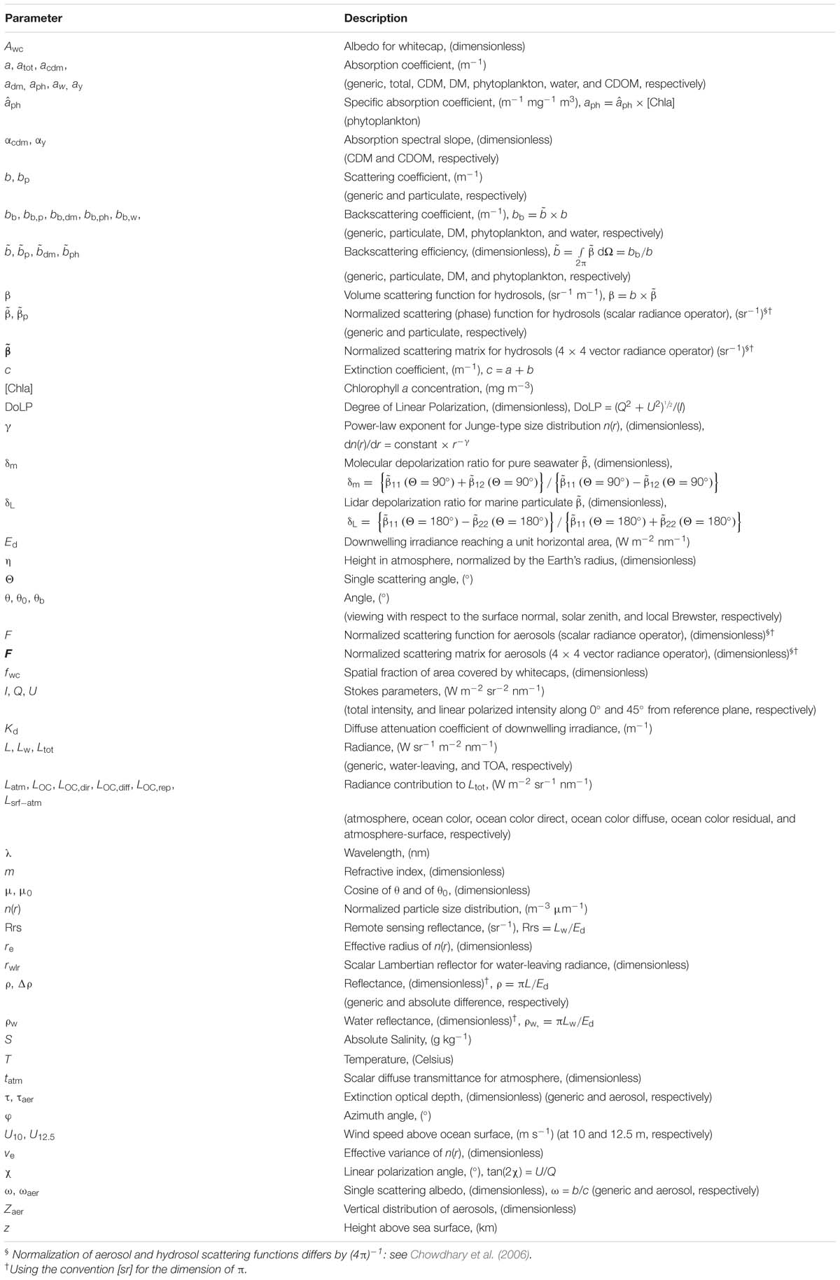
Table 2. List of parameters.
Both SPEXone and HARP2 instruments have smaller swaths and larger nadir-viewing pixel sizes, and they cover smaller parts of the UV-NIR spectrum, than the OCI. However, in addition to radiance measurements, SPEXone and HARP will also provide measurements of the linearly polarized radiance. Furthermore, both polarimeter instruments will look at each of their own pixels from multiple directions and will therefore capture angular features in the total and linearly polarized radiance. The swath for a SPEXone and HARP2 image will be 100 km and 1,556 km with a pixel resolution of ∼2.5 and ∼3.0 km, respectively. SPEXone will provide hyperspectral measurements of the total radiance at 2-nm spectral resolution, and of the Degree of Linear Polarization (DoLP) at 10–40 nm resolution, for the VIS-NIR regime covering 385–770 nm. On the other hand, HARP2 will provide measurements of the total and linearly polarized radiance in discrete narrow-bands (10–40 nm resolution) at four wavelengths in the VIS-NIR regime (440, 550, 670, and 870 nm). The radiometric SNR for an ocean scene in the VIS will be >800 and >200 at 10–40 nm resolution for SPEXone and HARP2, respectively. The corresponding DoLP accuracy for these instruments will be ≤0.3% and ≤1.0%. Each pixel of a SPEXone image will further be viewed from 5 angles at ±57°, ±20°, 0° from the satellite nadir view direction. HARP2 multi-angular measurements will cover the same angular range as SPEXone views but for more angles, i.e., for 60 angles at 670 nm and for 10 angles at the other three wavelengths.
SPEXone and HARP2 will therefore provide polarimetric data sets that have complementary strengths for better ocean, aerosol and cloud retrievals (see NASA, 2018b). That is, they complement each other in (i) swath coverage (ideally close to that of OCI for atmospheric correction); (ii) number of viewing angles (ideally ≥5 for atmospheric correction and for retrieval of aerosol properties and ice cloud scattering function, ≥10 for cloud thermodynamical phase retrievals, and ≥60 for water cloud droplet retrievals); (iii) spectral range (ideally include deep-blue channel for aerosol and cloud-top height retrievals) and spectral resolution (ideally matching OCI spectral resolution); (iv) SNR values (ideally matching OCI SNR); and (v) DoLP accuracy (ideally ≤ 0.5% for aerosol retrievals and ≤2% for cloud retrievals and atmospheric correction). Note that ideal polarimetric data sets could not have been achieved with a single instrument design at a practical cost; however, SPEXone and HARP2 will provide data sets that, when combined with OCI data, will help address the science goals for PACE well beyond its threshold requirements outlined in NASA (2018a).
Accurate calculations of the transport of solar radiant energy entering the Earth atmosphere are important for remote sensing of ocean color, aerosols, and clouds. They are needed to simulate the signal measured by an optical sensor, which may be carried onboard a satellite or deployed at any level in the ocean or atmosphere, to estimate the radiant contributions by various components in atmosphere-ocean systems, to characterize the properties (angular, spectral, and polarized) of the light field, and to develop inverse methods to retrieve the types and concentrations of optically active constituents. Diverse processes are involved and interact in various ways (e.g., elastic and inelastic scattering, absorption, fluorescence, and Fresnel reflection), which makes RT modeling of light in ocean-surface-atmosphere systems (AOS) a difficult issue. Realistic, precise, and reliable simulations depend on the proper treatment of the various processes and their interactions, all at the required spectral resolution (hyper-spectral in the case of PACE) and taking into account spatial heterogeneity.
In the following sections, we will focus on RT topics relevant to the work done by the 2014–2017 PACE Science Team for AOS models. The complexity of this work becomes apparent when listing some of the properties that have to be taken into account when performing RT computations in realistic AOS:
• Scattering and absorption by molecules, clouds and aerosols in the atmosphere
• Reflection and refraction by the ocean surface including the effects of surface roughness, shadowing, and multiple scattering
• Scattering by white caps, streaks, and floating substances such as oil slicks and biogenic films
• Scattering and absorption in the ocean by pure water, dissolved substances, and suspended matter
• Inelastic radiative processes including Raman scattering by ocean waters, fluorescence by dissolved organic matter, and fluorescence by chlorophyll.
Furthermore, there are geometric concerns that play a role such as the sphericity of the Earth, 3-dimensional variability in scattering properties such as isolated clouds and plankton blooms, azimuthal variability caused by e.g., oriented particles and wind-directionality of the ocean roughness, and the vicinity of land or sea-ice which leads to adjacency contamination of pixels viewed from space. Finally, there are numerical aspects that are important to consider for remote sensing (RS) applications such as the speed and validation of RT computations. The work done by our team touches upon many of these topics, the organization of which is presented as follows. In Section “2 History of RT Methods for AOS: A Brief Overview,” we provide a brief historical overview of the RT methods applied to AOS during the last few decades. In Section “3 Current RT Topics and Models: Heritage Studies, Discussions, and PACE Updates,” we focus on scattering in the ocean (“3.1 Ocean Body” section), by the ocean surface (“3.2 Ocean Surface” section), in the atmosphere (“3.3 Atmosphere” section), and by the entire AOS (“3.4 AOS models” section). In each of these subsections, we provide a brief overview of heritage work, followed by (when applicable) updated work performed by our team. For updated work, we differentiate between forward (FWD) RT studies that focus mainly on sensitivity analyses and/or simulating data sets, and inverse (INV) RT studies that involve also retrieval of PACE mission science products.
In what follows, we provide a brief historical overview of some of the RT studies performed on scattering of light in atmosphere-ocean systems. The list of studies does not do justice to the vast amount of work done on this topic by numerous researchers over a time span of many decades. For example this list focusses only on the progression of RT models and AOS models, i.e., models that provided a basis for subsequent refinements in FDW and INV RT models in other studies. Rather, the purpose of this list is to provide broad context for the research done by our team on RT methods and AOS properties to study PACE observations of oceans. We provide detailed historical information in the heritage overview part of each section. Methods and models that deal with RT in the atmosphere alone are reviewed by Hansen and Travis (1974), van de Hulst (1980), Lenoble (1985), and Stamnes (1986).
Chandrasekhar (1950) introduced methods to study reflected light and skylight of an atmosphere above a Lambertian surface. His methods were extended by Sekera (1961) to investigate scattering of polarized light in a Rayleigh atmosphere above a smooth ocean (see also Fraser and Walker, 1968). Later, Fraser (1981) and Ahmad and Fraser (1982) used another (i.e., Gauss-Seidel) method to study reflection of polarized light by a vertically inhomogeneous atmosphere that was bounded from below by a rough ocean surface.
A Monte Carlo approach was developed for an atmosphere above a smooth water surface plus water body (Plass and Kattawar, 1969, 1972), generalized later to include polarization (Kattawar et al., 1973) and a rough water surface (Plass et al., 1975, 1976; Tynes et al., 2001).
The method of successive orders of scattering without polarization was used by Raschke (1972) and later by Quenzel and Kaestner (1980) for RT computations in an atmosphere with aerosols and molecules above a rough ocean surface and ocean body. Chami et al. (2001) included polarization, but used a smooth ocean surface. (Chami et al., 2015) upgraded their code to include a rough ocean surface. Zhai et al. (2009, 2010) developed a polarized RT code based on this method that included both flat and rough ocean surfaces, which was later upgraded to account for inelastic radiative processes in ocean waters (Zhai et al., 2015, 2017a,b, 2018).
The adding method (van de Hulst, 1963) extended to include polarization by Hansen (1971) and Hovenier (1971) was used by Takashima (1974, 1975) for RT computations of polarized light in an atmosphere-surface system. This work was later updated to include an ocean body with a rough interface (Takashima, 1985; Takashima and Masuda, 1985; Masuda and Takashima, 1986, 1988).
Tanaka and Nakajima (1977) applied the matrix operator method, which is a variant of the adding method, without polarization for an atmosphere above a water body with a smooth surface. This method was later generalized to include a rough ocean surface by Nakajima and Tanaka (1983) and Fischer and Grassl (1984). Polarization was included for such systems by He et al. (2010) and Hollstein and Fischer (2012).
Dougherty (1989) used invariant imbedding techniques to study reflection without polarization by an ocean body covered by a smooth surface but no atmosphere. Mobley (1989, 1994) included a rough ocean surface in his Hydrolight program, and recently worked on including polarization for isolated rough ocean surfaces (Mobley, 2015) and ocean bodies (Mobley, 2018). Mishchenko and Travis (1997) employed a similar method including polarization for an atmosphere above a rough surface but no ocean body.
The Discrete-Ordinate RT method, introduced by Stamnes et al. (1988) for RT computations without polarization, was applied by Jin and Stamnes (1994) to an atmosphere above an ocean body with a smooth surface. Jin et al. (2004) subsequently included a rough ocean surface for such computations. Meanwhile Schultz et al. (1999) expanded this method to include polarization, which was applied by Sommersten et al. (2009, 2010) to atmosphere-ocean systems albeit with a smooth ocean surface.
Other authors opted to use a combination of the above-mentioned RT methods. For example, Chowdhary et al. (1995) applied the invariant imbedding method for the ocean body and used the adding method to include a rough ocean surface and atmosphere. Ota et al. (2010) used the Discrete-Ordinate RT method for homogeneous atmosphere and ocean layers, and used the matrix operator method to combine these results and to include a rough ocean surface. Xu et al. (2016) applied the Markov chain method for inhomogeneous layers and the adding method for homogeneous layers in the atmosphere and ocean, and used again the adding method to couple these layers and include a rough ocean surface. Polarization was taken into account in all of these combined RT methods.
The RT methods and AOS models listed above show a gradual trend from scalar computations for oceans with a smooth surface toward including polarization of light and considering rough ocean surfaces. However, most current RT methods still ignore inelastic radiative processes in the ocean, and most current AOS models still assume the atmosphere and ocean to be plane-parallel and horizontally homogeneous. In addition, most current RT methods apply (if not ignore altogether) simplified corrections for whitecaps, shadowing effects, and multiple scattering in rough ocean surfaces. Furthermore, much work still needs to be done in linking robust RT computations for realistic atmosphere-ocean systems to bio-optical modeling of ocean color. A driving constrain for PACE is to retrieve water-leaving radiance to better than 5% (10%) in the VIS (UV), and to retrieve properties of the atmosphere and ocean from this radiance with better accuracies than from heritage ocean color and atmosphere sensors. This requires among others more flexible bio-optical models that can also be applied to UV radiance, more realistic scattering matrices for marine particulates, better estimates of (in)elastic scattering and absorption by pure sea water, and less assumptions made for AOS models. Finally, there are no extended, peer-reviewed and accurate tabulated RT bench-mark results for fully coupled atmosphere-ocean models to validate any of the above-mentioned methods to accuracies consistent with PACE measurements. The next section provides a summary of work done by the 2014–2017 PACE Science Team that touches upon many of these topics.
Radiative transfer models describing the angular distribution of the total and polarized radiance that is singly scattered by marine particulates can be classified into (A) those derived from measurements, (B) those computed for predefined particulates, and (C) those approximated with analytical expressions. Among the most widely used RT models belonging to class A are the early tabulated normalized scattering function ( ) data provided by Petzold (1972), and the early tabulated normalized scattering matrix () data provided by Voss and Fry (1984). Such models have the clear advantage of producing realistic bidirectional reflectance distribution functions (BRDFs) for water-leaving radiance in multiple scattering computations. However, due to their limited coverage of water types and/or averaging over data sets, they cannot replicate the variability in bidirectional scattering by marine particulates seen in laboratory (e.g., Volten et al., 1998; Witowski et al., 1998) or ocean (Mobley et al., 2002; Sullivan and Twardowski, 2009; Zhang et al., 2011; Twardowski et al., 2012) measurements. In addition, the Petzold volume scattering function data appear to be affected by an error such as stray light reflections in the near backward, which becomes prominent/obvious in his clear water dataset which do not agree with theory, other measurements, or satisfy closure with simulated apparent optical properties (i.e., properties that depend on the ambient light field). The work by Sullivan and Twardowski (2009) represents another example of Class A models. Here, the focus is placed on approximating the shape of the scattering function in the backscattering hemisphere based on extensive field measurements. Note that their results agree with the analytical Fournier-Forand scattering functions discussed below for Class C models.
Radiative transfer models belonging to class B typically assume the particles to be spheres that follow a Junge-type (power-law) size distribution with exponent γ (see Table 2) ranging between 3 ≤ γ ≤ 5 (Stramski and Kiefer, 1991). Furthermore they typically assume such particles to be homogeneous with real refractives index m that can be grouped into two or more classes (Gordon and Brown, 1972; Zaneveld et al., 1974), i.e., either falling between 1.02 ≤m ≤ 1.10 for plankton-like organic particles (Spinrad and Brown, 1986; Aas, 1996) or between 1.15 ≤m ≤ 1.25 for mineral-like inorganic particles (Woźniak and Stramski, 2004). Variations in the distribution of singly scattered light can be replicated with these models by varying γ and/or m for a single polydisperse population (Twardowski et al., 2001), or by varying the mixing ratio of two (or more) modes of polydisperse particles that each have their own fixed set of (γ, m) values (Chowdhary et al., 2012; Kopelevich, 2012). Because of their variation with γ and m, class B models can be used to either mimic changes in particulate scattering functions in (empirical) remote sensing studies (Morel et al., 2002; Chowdhary et al., 2006; Ibrahim et al., 2016), or to retrieve m and/or γ from remote sensing observations (Loisel et al., 2008; Kostadinov et al., 2010). However, the goodness of RT and retrieval results obtained with class B models depends on the shape and internal structure assumed for marine particulates (Stramski et al., 2004). For example assuming spherical shapes for phytoplankton can create significant biases in the backscattering direction (Clavano et al., 2007), which become even larger when ignoring internal structures such as membrane walls and organelles (Kitchen and Zaneveld, 1992; Matthews and Bernard, 2013; Sun et al., 2016; Duforêt-Gaurier et al., 2018). Recently, Twardowski et al. (2012), Zhang et al. (2012, 2013, 2014b), Zhang and Gray (2015), and Xu G. et al. (2017) have started addressing the first issue by incorporating non-spherical (i.e., hexahedral) shapes for marine particulates in their retrieval studies of scattering functions. Other efforts to account for particle non-sphericity in RT simulations of underwater light are described by Gordon et al. (2009) and Gordon (2011) for the scattering properties of detached coccoliths, by Zhai et al. (2013) and Bi and Yang (2015) for the scattering properties of whole coccolithophores, and by Fournier and Neukermans (2017) and Neukermans and Fournier (2018) for the scattering properties of both detached coccoliths and whole coccolithophores. In addition, Organelli et al. (2018) started using coated spheres in RT computations to force closure with underwater light particulate backscattering and attenuation measurements, whereas Poulin et al. (2018) compared the performance of coated spheres and hexahedral shapes in closure studies of phytoplankton cultures.
Radiative transfer models belonging to class C use simple analytical expressions, instead of rigorous computations, to obtain scattering functions for marine particulates. Among the earliest and simplest models belonging to this class are (linear combinations of) Henyey-Greenstein functions (Henyey and Greenstein, 1941). These functions can be parameterized (Plass et al., 1985; Haltrin, 2002) in terms of the particulate backscattering efficiency (defined in Table 2), but typically are not representative over the full angular range. Another, more widely used model belonging to this class is the Fournier-Forand scattering function (Fournier and Forand, 1994; Fournier and Jonasz, 1999; Mobley et al., 2002). This function is based on fundamental physical principles instead of empirical fitting, can be parameterized in terms of γ and m, and therefore retains the link to physical properties of marine particulates just like class B models. Mobley et al. (2002) further developed an approach to parameterize Fournier-Forand phase functions in terms of , where γ and m are effectively assumed to covary. Fournier-Forand phase functions are exceptionally accurate for a broad range of particle types. Sullivan and Twardowski (2009) showed a remarkably consistent shape for the particulate fraction in volume scattering function measurements collected in ten disparate field sites around the globe, including both Case I and II type waters. The observed phase function shape was consistent with analytical Fournier-Forand phase function shapes when the Mobley et al. (2002) approach was followed over the full natural range for polydispersions, i.e., ranging from 0.003 to 0.03. The Sullivan and Twardowski (2009) phase functions shape has recently been shown to be applicable even in massive cyanobacterial blooms in Lake Erie (Moore et al., 2017). Simulations of BRDFs based on this single shape perform as well or better than more complex functions when compared to direct BRDF measurements, particularly in complex Case II waters (Gleason et al., 2012). This is consistent with previous works showing the BRDF for ocean color remote sensing is, to first order, controlled by the shape of scattering in the backward direction (Morel and Gentili, 1991, 1993; Gordon, 1993; Zaneveld, 1995; Morel et al., 2002). However, with the notable exception of Kokhanovsky (2003), class C models do not provide such parameterizations for the full (4 × 4) scattering matrix for representative polydispersions that are needed to perform RT computations of polarized underwater light. We remark that many models belonging to class A or B do provide scattering matrices, albeit not parameterized in terms of , γ or m.
Finally, there are hybrid RT models that use the scattering matrices of class A models except for first normalizing them by their scattering function, and then multiplying them by the parameterized functions of class C models (e.g., Adams and Kattawar, 1993; Zhai et al., 2010; You et al., 2011; Gu et al., 2016; Xu et al., 2016). Such hybrid models combine the advantages of class A for realistic scattering matrices and of class C models for variations in the scattering function. However, they still lack variability for the other scattering matrix elements. A potential solution to mitigate this problem is to adopt the parameterization provided by Kokhanovsky (2003) for the other scattering matrix elements. In this approach, taken by Zhai et al. (2015), the parameterization of the other scattering elements occurs in terms of the underwater light DoLP instead of , γ and m. But to make this approach completely self-consistent for all scattering matrix elements, one still needs to relate variations in DoLP to variations in , γ and m.
To investigate the relative importance of plankton shapes and internal structures in INV RT studies of underwater light scattering, computations were initialized to compare the scattering matrices for four classes of particles: (I) homogeneous and spherical; (II) homogeneous and non-spherical; (III) inhomogeneous and spherical; and (IV) inhomogeneous and non-spherical (Chowdhary, Liu et al., unpublished). Class I particles are known to scatter less light in the backward direction than class II, III, and IV particles. It has been suggested that this plays a role in explaining the so-called missing backscattering enigma in underwater light scattering computations for micrometer-sized marine particles when compared to underwater light measurements (Stramski and Kiefer, 1991; Stramski et al., 2004). While scattering by sub-micron particles is favored by some to explain this enigma (Stramski and Wózniak, 2005) even when taking non-sphericity into account (Zhang and Gray, 2015, but see Clavano et al., 2007), one cannot ignore the large increase in backscattered light when taking internal structures such as wall membranes and organelles into account (Meyer, 1979; Bernard et al., 2009; Dall’Olmo et al., 2009; Sun et al., 2016; Duforêt-Gaurier et al., 2018; Organelli et al., 2018).
Details of the four classes of particles considered thus far are illustrated in Figure 1A. In this panel, chloro, cyto, mito, nucl, and vac stand for chloroplast, cytoplasma, mitochondria, nucleus, and vacuole, respectively. The surface-equivalent diameter of each particle is kept at 1 μm. The diameter of the organelles varies between 0.3 (mito), 0.4 (nucl, vac) and 0.5 μm (chloro), and thickness of the membrane wall (if present) is 0.1 μm. Also shown are scattering matrix examples in Figure 1B that were computed for some of these particles for a wavelength of 0.55 μm. These initial computations show that (i) internal structures increase the radiance scattered in the backward direction by several factors compared to variations in particle shape; and (ii) only variations in particle shape can create the magnitude of deviations from unity in the (2,2) scattering matrix element seen by Voss and Fry (1984). Observation (i) is consistent with the scattering matrix analyses by Quinby-Hunt et al. (1989). It strongly suggests that, in addition to colloid particles, one needs to consider internal structures of plankton-like particles when comparing underwater light scattering computations with backscattering efficiency data for particulate scattering [this is also supported by the bb,p (given in Eq. 1) data analyses in Dall’Olmo et al. (2009)]. Observation (ii) further suggests that ocean depth profiles of Lidar Depolarization Ratio δL (defined in Table 2) obtained from airborne observations (Hu et al., 2016) such as the one shown in Figure 1C are more sensitive to particle shape than to particle inhomogeneity. In addition, computations of and δL performed for an ensemble of Class II particles with an equi-probable distribution of spheroid shapes show (see Figure 1D) that they exhibit quasi-orthogonal sensitivities to variations in the size and bulk composition of large marine particulates. Note also from Figures 1C,D that HSRL retrievals of δL are consistent with γ > 4 when assuming equi-probable distributions of spheroid shapes. The next steps in this line of research consist of obtaining representative and optically relevant shapes and internal structures of plankton particles that can be used in INV RT studies to retrieve and δL from in situ and lidar measurements, respectively. Emerging particle characterization methods such as in situ holographic imaging (Talapatra et al., 2013; Nayak et al., 2017) are also expected to aid in development and validation of such a model.
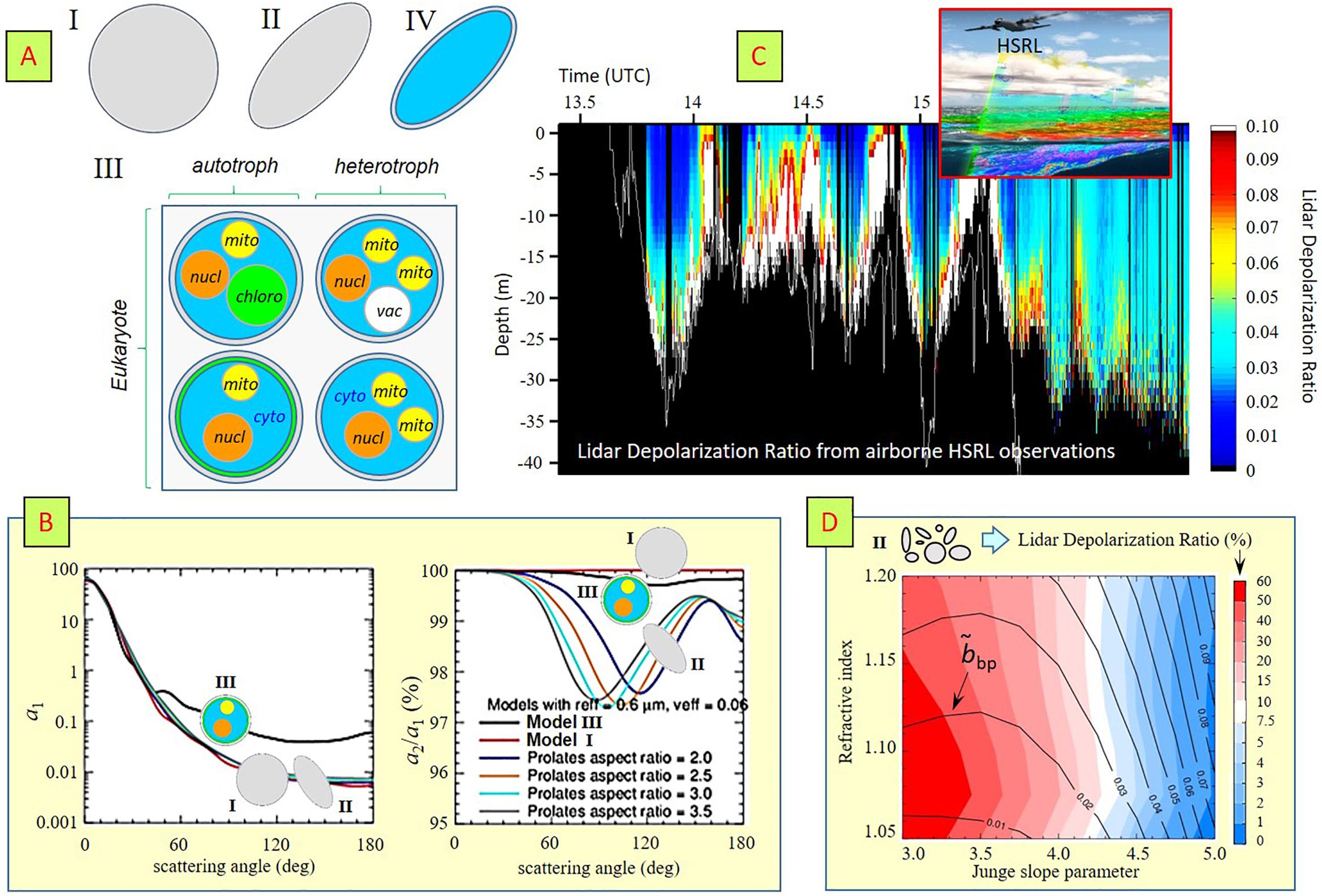
Figure 1. (A) Particulate classes considered for plankton particles. Class I = spherical and homogeneous; Class II = non-spherical and homogeneous; Class III = spherical and inhomogeneous, Class IV = non-spherical and inhomogeneous. Class III and IV models contain a membrane wall and are filled with cytoplasm (“cyto”). Class III models contain one or more of the following organelles: chloroplast (“chloro”), mitochondria (“mito”), nucleus (“nucl”), vacuole (“vac”). (B) Scattering matrix element (1,1) (left diagram: a1) and normalized scattering matrix element (2,2) (left diagram: a2/a1) computed for Class I, II, and III particles. (C) Ocean depth profile of lidar depolarization ratio δL example obtained by HSRL at λ = 532 nm during the NAAMES field campaign. The lower white curve marks the physical ocean bottom. (D) Lidar depolarization ratios and backscattering efficiencies computed at λ = 550 nm for randomly oriented Class II particles as a function of Junge size distribution exponent and refractive index.
Recent work has verified the excellent accuracy of the Fournier-Forand analytical phase function in describing shapes of across the angular range near zero to 170°. Field measurements of the quantity β ≡ b × , i.e., of the volume scattering function (VSF), have been made using a combination of a custom Multi-Angle SCattering Optical Tool (MASCOT) resolving the VSF from 10° to 170° in 10° increments, and the Sequoia Type-B LISST resolving the near-forward VSF from 0.079° to 12.9° in 32 log-spaced increments. Fournier-Forand phase functions can be least-squares fit directly to these measured VSFs. When doing this, root-mean-square (RMS) errors <10% are typically observed over the full 6 order of magnitude VSF range. Despite the excellent accuracy of the Fournier-Forand analytical model, a systematic underestimation can still be observed in some cases in the ∼1° to 70° range. This underestimation was also recently noted by Harmel et al. (2016) in measurements of polydisperse Arizona Road Dust suspensions. The systematic nature of the bias indicated there may be the possibility of invoking a fitting method that may yet enhance accuracy. In collaboration with Dr. Tim Moore (UNH), a two cluster model was developed to fit VSFs that was able to effectively fit the mid-angle range, reducing RMS errors relative to fitting the Fournier-Forand function, with RMS errors in some cases decreasing from 17–18% to 3–7% (Twardowski et al., in preparation) (Figure 2). For INV RT models dependent on VSF shape (Zaneveld, 1995; Twardowski and Tonizzo, 2018), such a statistical model introduces one additional variable describing the mixing of the two clusters to reproduce the shape of the complete VSF, or it can be used to extrapolate or interpolate phase function shape from limited ancillary scattering measurements.
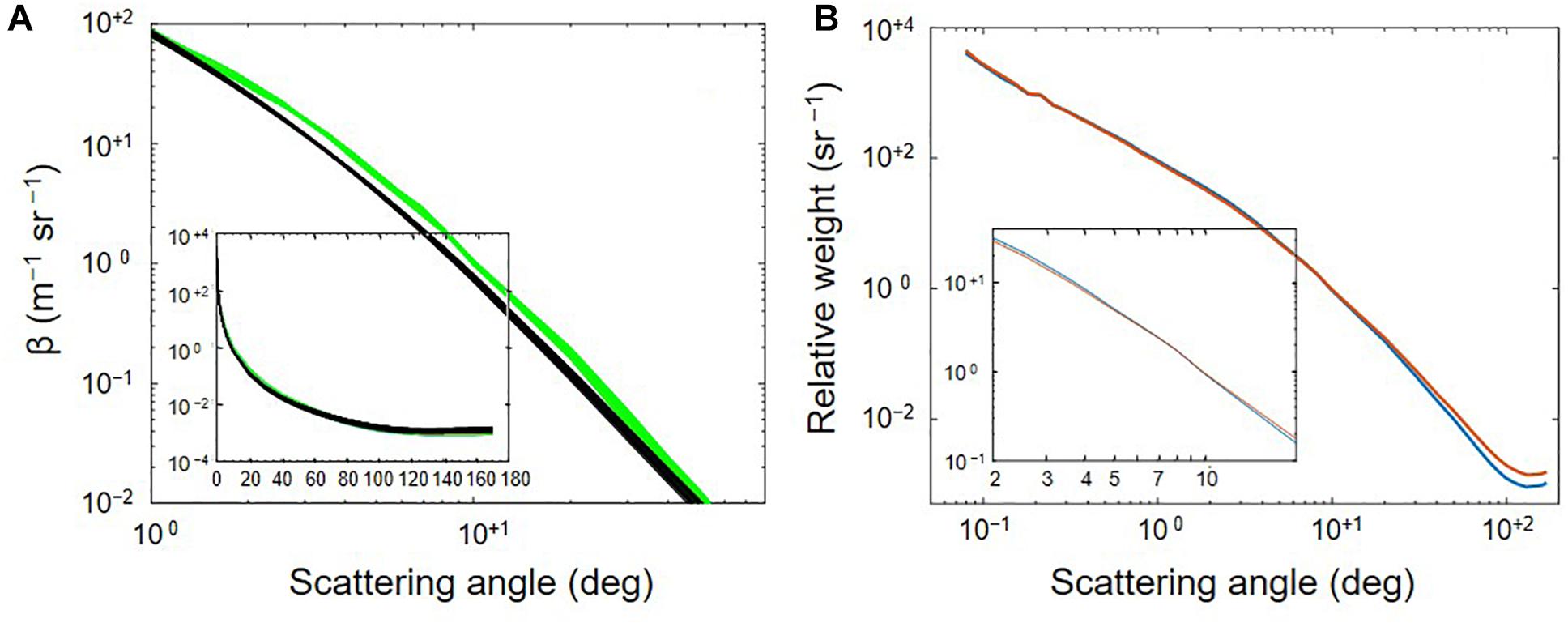
Figure 2. (A) Fifteen, 1-m binned VSFs (green) from a single profile collected in the New York bight 11/2007, highlighting the ∼1° to 70° range where Fournier-Forand phase function fits (black) systematically underestimate. Inset shows semi-log scale over full range. RMS error for the profile was 17.5%. (B) Two fitting clusters for data collected in the New York bight, derived using the method of Moore et al. (2009, 2014, see text). The vertical axis (i.e., relative weight) corresponds to β normalized by its integrated value over available scattering angles. One cluster exhibits about twice the amount of scattering in the backward direction relative to the other. There is also a cross-over point at 7° (see inset). Fitting the same profile data from panel (B) with the 2 clusters model results in an improved RMSE of 7%.
The two clusters are purely statistical quantities, i.e., they are two functions that, when mixed, minimized errors in describing the shapes of VSFs. Applying these functions to a much larger MASCOT VSF data set resulted in very low RMS errors, <10% in all cases except Hawaii, where signal-to-noise issues in very clear water are also significantly impacting RMS error (Table 3). Results suggest naturally observed VSFs in the 10° to 170° range may be represented with excellent accuracy with a function having only two degrees of freedom, with one variable being essentially a concentration metric and the other a mixing (shape) metric. While the two cluster fitting method provided optimal fits, a drawback is the loss of any physical meaning of the fit. The result of the two cluster fitting method are two amplitudes, one for each cluster, whereas the Fournier-Forand fits result in physically meaningful bulk refractive indices m and particle size distribution slopes γ, along with a scaling factor representing concentration.
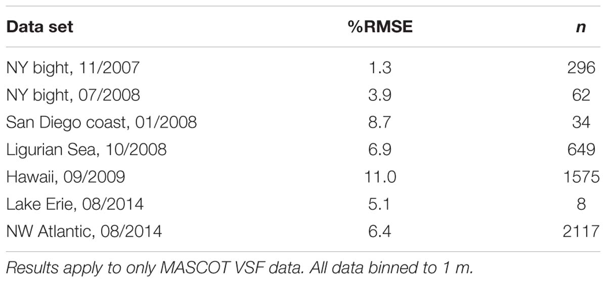
Table 3. Percent (%) RMSE results after fitting two clusters to VSF data collected around the globe.
Different from the idealized Fournier-Forand phase function (Fournier and Forand, 1994), simplified two-parameter models (Chowdhary et al., 2012; Kopelevich, 2012), or statistical two cluster approach described above, Zhang et al. (2011) and Twardowski et al. (2012) developed a theoretical approach to represent scattering functions using various particle subpopulations, each of which corresponds to an optically unique particle species that follows a log-normal size distribution n(r). In Zhang et al. (2011), the particles assume spherical shapes and in Twardowski et al. (2012), the particles assume non-spherical shapes consisting of asymmetrical hexahedra for inorganic mineral particles (Bi et al., 2010) and Lorenz-Mie theory for coated bubbles (Czerski et al., 2011; Zhang et al., 2011). Later, asymmetrical hexahedra shape was applied to organic particles (Zhang et al., 2012). Through sensitivity analyses over the ranges of published size distributions and composition for oceanic particles, extensive libraries of distinctive particle phase functions have been built to represent the angular scattering and to serve as fingerprints for various oceanic particle species through inversion (Zhang et al., 2011, 2012; Twardowski et al., 2012).
With this particle phase function library, a measured VSF can be inverted to identify and quantify the scattering coefficient and the size distribution of the particle species (Figure 3A). The particle subpopulations or species identified via inversion represent the biogeochemical origin to the observed angular scattering. This approach has been applied to VSFs measured by the MASCOT mentioned above and another prototype volume scattering function sensor, Multispectral Volume Scattering Meter (MVSM), which resolves VSFs from 0.5° to 179° in 0.25° increments at eight wavelengths (Lee and Lewis, 2003). The results have been successfully validated in several studies with independent measurements. That is, the bulk particle size distribution n(r) derived from the VSF-inversion is consistent with the Laser in situ Scattering and Transmissometery (LISST)-based estimates for particles of sizes greater than 2.5 μm, with an overall agreement of within 10% evaluated in three coastal waters (Chesapeake Bay, Monterey Bay, and Mobile Bay) (Zhang et al., 2012; also see Figure 3C). Czerski et al. (2011) and Twardowski et al. (2012) estimated the dynamics of bubble populations of sizes < 30 μm during active wave breaking, where the optical volume scattering and acoustical determinations agreed well. Using the filter pore size as a threshold, Zhang et al. (2013) partitioned the inverted subpopulations into particulate and “dissolved” fractions (see Figure 3B), and further extracted phytoplankton particles using refractive indices m = 1.04 and 1.06 (Aas, 1996) from the particulate fraction. In support of their VSF inversions, Zhang et al. (2013, Figure 2) used an observed relationship between phytoplankton cell sizes and chlorophyll concentration to estimate the total chlorophyll concentration from their retrieved phytoplankton sizes and compared it favorably (Pearson correlation coefficient r = 68%) with chlorophyll estimates obtained from High-Performance Liquid Chromatography (HPLC) measurements. Similarly, Zhang et al. (2014b) estimated the mass for particulate inorganic matter and particulate organic matter, with results comparing well with the laboratory gravimetric determinations in both Monterey Bay and Mobile Bay.
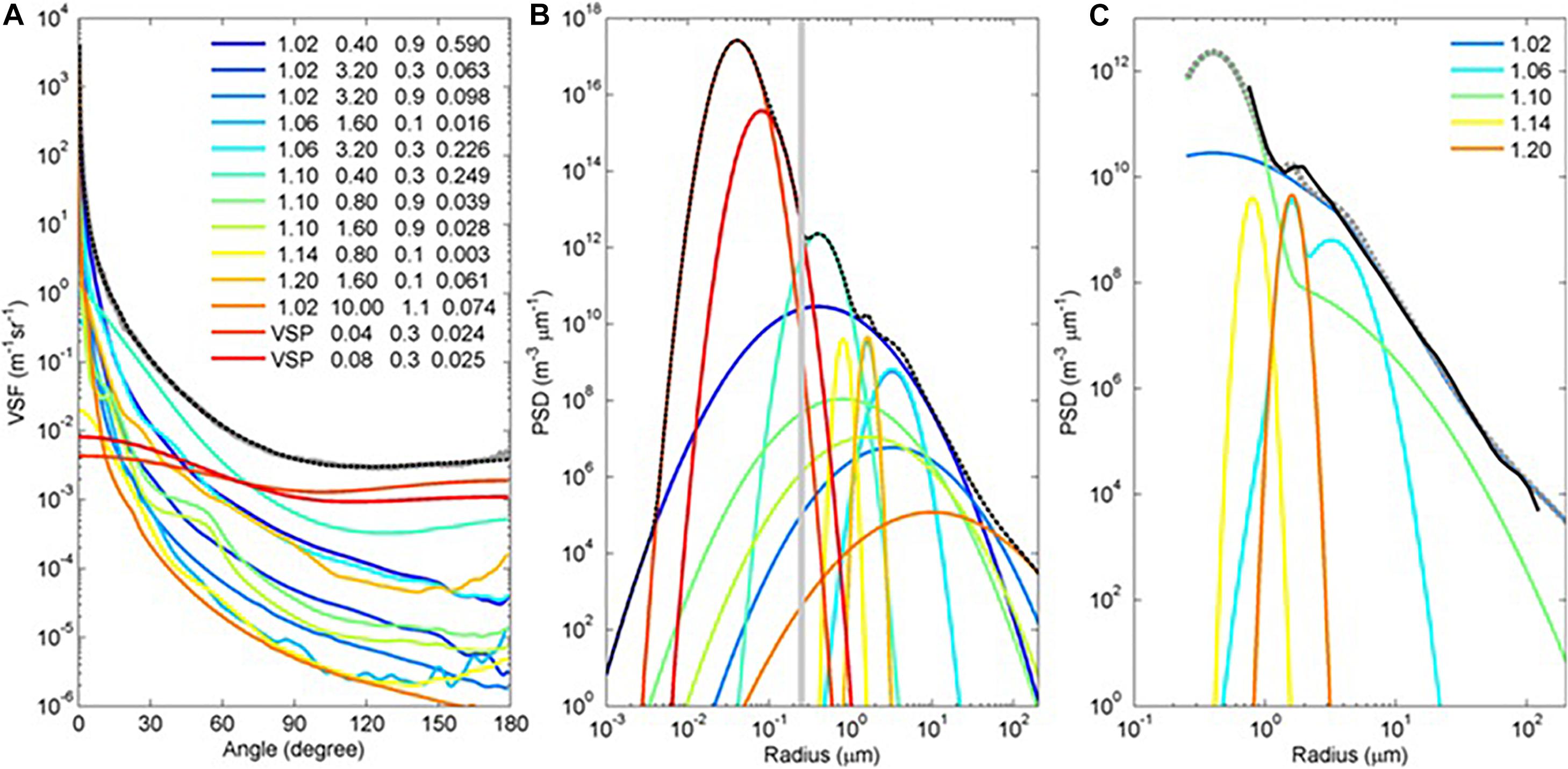
Figure 3. An example demonstrating representing a measured VSF using various particle subpopulations. (A) The measured VSF (gray line) was disaggregated into subpopulations, whose corresponding refractive index, the mode size and standard deviation, and the scattering coefficient are shown in the legend. The dotted black line is the reconstructed VSF from these subpopulations. (B) Log-normal size distributions estimated for each of the subpopulations identified in panel (A). The vertical gray line represents the filter size that commonly used in oceanography to partition particles into particulate and dissolved fractions. (C) The size distribution of subpopulations the particulate fraction are grouped by the refractive indices (shown in the legend). The dotted gray line is the bulk size distribution estimated by summing individual subpopulations. The black line is the size distribution independently derived from the LISST for comparison.
Over the entire angular range of the volume scattering, varying particle composition can change the particle VSF in terms of its shape. For example, the change of forward scattering VSF, when normalized by the total scattering coefficient could vary over 3–4 orders of magnitude. However, within the angular range of 90° to 180°, there are different findings regarding shape variability. Sullivan and Twardowski (2009) found that the backscattering shape as revealed from the MASCOT measurements was relatively constrained. That is, they found errors of 5% or less in fitting a single shape function from 90° to 170° for an extensive, global VSF data set, suggesting a more or less invariant backscattering shape. In contrast, Zhang et al. (2017) has recently found that backscattering shape, i.e., VSFs from 90° to 180°, as measured by the MVSM in three coastal waters around United States and in North Atlantic Ocean, varied up to a factor of two (Figure 4B). These disparate findings, which are based on measurements from two different prototype instruments over different waters, have yet to be resolved. The backward shape has a strong influence on the remote sensing BRDF, where about 97% of total variability observed in remote sensing reflectance (Rrs – see Table 2) over different viewing angles is due to the change in the detailed VSF shape over the backward angular range (Xiong et al., 2017). On the other hand, only 27% variability in the Rrs BRDF is attributable to the backscattering efficiency . Therefore, to meet the 5% PACE retrieval requirement for water-leaving radiance, we need to further improve our knowledge on backward variability of VSF to constrain the estimate of BRDF, which is particularly important for the PACE OCI instrument that has a wide field of view. Both field observations and theoretical studies have also found the backward shape of the VSFs of oceanic particles, defined as βp (θ)/bb,p (where bb,p is the particulate backscattering coefficient, cf. “3.1.2 Bio-Optical Models” section), exhibits minimum shape variability in the backward direction (Oishi, 1990; Zhang et al., 2014a). Boss and Pegau (2001) showed that the minimum variability at 120° can be explained from mixing of particulate VSFs and salt water. Recently, however, Zhang et al. (2017) have suggested this minimum variability angle represents the intersection of two backscattering-normalized VSFs, one for particles of sizes smaller than the wavelength of light and the other for particulate sizes larger than the wavelength of light (Figure 4A). For each of the two end members, the backscattering shape can be analytically derived (Zhang et al., 2017). They also found that 90% of variability of the observed VSFs from 90° to 170° (Figure 4B) can be reproduced by this two-component model (Figure 4C). The minimum variability of scattering observed around 120° is intriguing and deserves further investigation.
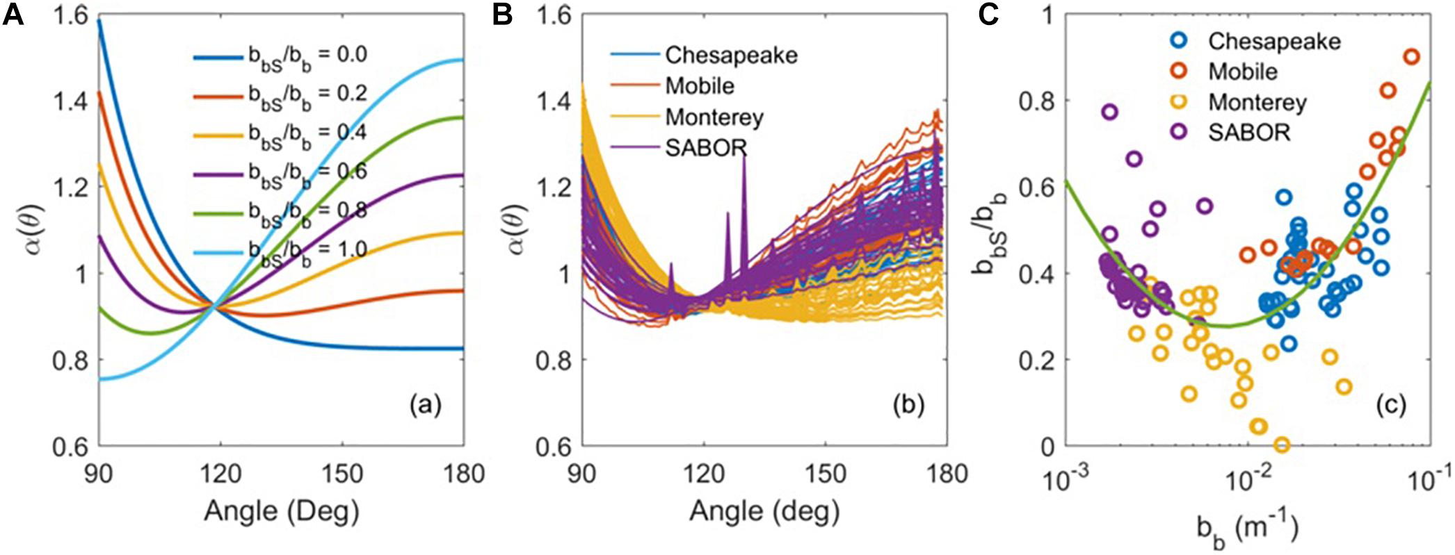
Figure 4. (A) The variation of hypothetical particle scattering shapes (VSF at angles 90°–180° normalized by the backscattering coefficient) constructed by linear mixing of the two end members. The legend shows fractional bb contributed by small particles. (B) The particle backscattering shapes measured in coastal waters of Chesapeake Bay, Mobile Bay, and Monterey Bay and during the SABOR cruise in North Atlantic Ocean. (C) The mixing ratios estimated by applying the two-component model in panel (A) to measured VSF shapes in panel (B) are shown as a function of particle backscattering coefficients.
Despite its fundamental role in ocean color remote sensing, the field-based observation of VSFs is still limited, which in turn circumscribes our understanding of the natural variability of angular scattering by oceanic particles and our ability to better model and/or retrieve these particles from the PACE mission. Efforts are being undertaken to expand the observation of particulate VSFs to a variety of waters with additional instruments and to improve our knowledge on the shape of particulate VSFs, particularly in the backward angles.
Bio-optical models play a central role in characterizing ocean color spectra. Firstly, they identify inherent (i.e., independent) underwater light optical parameters that drive (and can therefore be retrieved from) the flux and spectrum of water-leaving radiance. These IOPs are (Gordon et al., 1975; Preisendorfer, 1976; Morel and Prieur, 1977) the spectral absorption and scattering coefficients a and b, respectively (the sum of which gives the attenuation coefficient c ≡ a + b), and the backscattering efficiency which was mentioned earlier in Section “3.1.1 Particulate Scattering”. IOPs are tightly related to the fundamental RT quantities for underwater light scattering computations, i.e., the single scattering albedo ω (ω ≡ b/c), the normalized scattering function ( ≡ ∫ 2π dΩ where Ω stands for solid angle that is integrated over the backscattering hemisphere), and the optical thickness τ (τ ≡ ∫ c dz where z stands for physical thickness) of the ocean body. The RT quantities themselves vary with the abundance (i.e., number density), physical (e.g., size distribution and morphology) and chemical (e.g., organic versus inorganic) properties of suspended and dissolved marine matter. Hence, in principle, it is possible to retrieve e.g., the size distribution of marine particulates from IOPs. One of such retrieval was performed for phytoplankton by Kostadinov et al. (2009), who for this purpose assumed homogeneous spheres for the morphology of plankton particulates.
Secondly, bio-optical models provide a link between IOPs and the biological state of the ocean. That is, IOPs are commonly subdivided into contributions by water, phytoplankton, non-algal particles (NAP), and color dissolved organic matter (CDOM). Each of these contributions, except for water, are then represented by the product (or a sum of products) of a pre-defined specific spectrum (i.e., an eigenvector) and the amplitude of this spectrum (i.e., its eigenvalue). In the first generation of ocean color retrievals, it was customary (Morel, 1988; Morel and Maritorena, 2001) to parameterize the eigenvectors and eigenvalues of IOPs a, b and in terms of just 1 parameter: the concentration of Chlorophyll a ([Chla]), which is a photosynthetic pigment found in phytoplankton. Thus, the assumption made here was that the abundance and properties of each constituent in oceanic water (including NAP and CDOM) covaried with the concentration of phytoplankton. Such oceanic waters were collectively classified as Case I waters, while the remaining ocean waters, where the properties did not correlate well with chlorophyll and where inorganic matter could be important, were collectively classified as Case II waters. Case I waters were found to statistically represent open oceans well. Given that IOPs are tightly related to RT quantities (see discussion above), it is therefore possible for such oceanic waters to link variations in [Chla] to variations in the physical properties of marine particulates. For example, Kostadinov et al. (2009) found that their retrieval of pico (small-sized) and micro (large-sized) phytoplankton are highly correlated with small and large values of remotely sensed [Chla], respectively. However, bio-optical models are commonly derived from empirical fits to data that can be extremely noisy – see e.g., Bricaud et al. (1998) for phytoplankton absorption coefficient aph, and Huot et al. (2008) for b and . Hence, the goodness and application of correlating the retrieval of physical properties such as phytoplankton size to the retrieval of biological properties such as [Chla] depends on the assumptions (e.g., plankton morphology) and uncertainties (e.g., scatter in bio-optical relations) associated with each retrieval.
The initial custom of classifying ocean waters into two opposite cases, and closely tying one of them to [Chla], has evolved over the past 2 decades (Mobley et al., 2004). For example, Aeolian dust storms are known to be an important source for suspended mineral particles in the open ocean (Johnson et al., 2010). The abundance and properties of these particles clearly do not co-vary with [Chla], although they provide nutrients that may lead to plankton blooms (Behrenfeld et al., 1996; Behrenfeld and Kolber, 1999; Boyd et al., 2000, 2009; Bishop et al., 2002). Plankton blooms themselves such as coccolithophore outbreaks can lead to excessive amounts of suspended mineral particulates whose scattering properties do not co-vary with [Chla] either (Balch et al., 2004). Furthermore, the bio-optical relationship between [Chla] and the absorption by CDOM, which is created by a variety of processes (Nelson and Siegel, 2013), is not only less tight than between e.g., [Chla] and b (Morel, 2009), but it also deteriorates quickly for UV wavelengths (Morel et al., 2007a). In addition, the temporal cycles of CDOM and [Chla] do not exactly match each other (Hu et al., 2006; Lee et al., 2010). The current generation of bio-optical models acknowledges these concerns by relaxing the interdependency of IOPs. Werdell et al. (2013a, 2018) provide an overview of the current state of bio-optical models. That is, eigenvalues of IOPs do not necessarily co-vary with [Chla] and eigenvectors may be either prescribed or retrieved/computed from ocean color data in real time. The implication is that the RT quantities {ω, τ, } used to perform underwater light scattering computations then also do not necessarily co-vary with [Chla] or even with one another. Such relaxations in IOPs remain to be adopted in current generation RT studies of polarized light emerging from AOS models (e.g., Chowdhary et al., 2006; Hasekamp et al., 2011; Knobelspiesse et al., 2012; Zhai et al., 2015). In addition, the (default) IOPs discussed in Werdell et al. (2013a) are for the wavelength (λ) range of 400–700 nm. This range, which was originally proposed by IOCCG (International Ocean Color Coordinating Group) in its IOCCG report #5 (2005) for the creation of synthetic IOP data, needs to be extended into the UV for RT studies to be applicable to PACE observations (see Werdell et al., 2018).
Heritage bio-optical models have traditionally been used in RT studies to invert ocean spectra. For remote sensing observations from space, one has to first retrieve and subsequently subtract the contribution of atmospheric scattering in order to obtain these ocean spectra. Such retrievals of atmospheric scattering contribution are also a requirement for the inversion of aerosol properties from spaceborne observations over ocean. Two types of methods can be adopted to accomplish this separation of atmospheric and oceanic signals in space-borne observations. In the first method (called the 2-step approach), this is done by focusing on the spectral variation of radiance in the NIR and/or the SWIR where the ocean becomes black (because of strong absorption by pure sea water) to select an aerosol model that is capable of reproducing this radiance. This method, which has historically been used for atmospheric correction of spaceborne ocean color observations (Gordon and Wang, 1994b; Gao et al., 2000; Wang and Shi, 2007; Ahmad et al., 2010), does not require any a priori information of the ocean. Hence in this method, bio-optical models are only used to invert oceanic signals after characterizing the atmospheric signal. For more details on this method, see IOCCG (2010) and Frouin et al. (2019). In the second method (called the 1-step approach), the atmospheric scattering contribution is retrieved from the spectral variation of radiance in the NIR/SWIR and in the VIS. Here, one needs bio-optical models to account for the contribution of water-leaving radiance in the VIS as part of charactering atmospheric signals. The bio-optical models used in this second method can be divided into type (i) and type (ii) models, depending on their purpose. Type (i) models are used to only approximate water-leaving radiances for the purpose of improving the retrieval of aerosol properties in the VIS (note though that the results of such aerosol retrievals can subsequently be used to perform atmospheric correction for retrieval of the actual ocean color). Such use of bio-optical models is seen in Xu et al. (2016). On the other hand, the purpose of type (ii) models is to not only retrieve aerosol properties but to also retrieve ocean properties at the same time. This approach is used by Chowdhary et al. (2012). Type (ii) models are therefore similar to (if not the same as) the bio-optical models used to invert ocean spectra in the 2-step approach described above. Both Chowdhary et al. (2012) and Xu et al. (2016) pioneered the use bio-optical models to analyze polarimetric remote sensing observations over oceans. However, they both adopted a simple bio-optical model, i.e., one where all the IOPs are parameterized in terms of [Chla] only. Such models cannot account for natural variations in water-leaving radiances (which can be larger than PACE’s retrieval threshold value of 5%; cf. “1.1 The PACE Mission” section) that occur for a given [Chla]. This does not necessarily pose a problem for type (i) bio-optical models that are only used to improve aerosol retrievals in the VIS. Note that to mitigate possible errors of single-parameter-based bio-optical models, Xu et al. (2016) allow adjustments of water-leaving radiance in their type (i) bio-optical model by adding Lambertian terms. However, type (ii) bio-optical models are used to also retrieve IOPs, and require therefore more parameters to describe complex waters. The accuracy requirements for IOP retrievals are not yet defined for PACE (cf. “1.1 The PACE Mission” section). Hence, evaluating the IOP retrieval performance of type (ii) bio-optical models occurs by comparing with co-located independent IOP measurement sets. Following the evolution of bio-optical models discussed in the preceding heritage section, the current PACE Science Team focused on incorporating more parameters in both type (i) and (ii) bio-optical models for analyses of VIS polarimetric observations.
The hydrosol model employed by Chowdhary et al. (2012) is based on using a [Chla]-driven type (ii) bio-optical model to constrain the RT properties of a mixture of plankton and detritus particles. This so-called D-P (Detritus-Plankton) hydrosol model, which can be applied to underwater scattering of polarized light and which reproduces classical (i.e., statistically averaged) “Case I” ocean color variations, is discussed in detail by Chowdhary et al. (2006). To relax the dependency on [Chla], the parameterizations of IOPs in the D-P hydrosol model were updated to accommodate the retrieval of three separate IOPs. The result of these updates is the second generation D-P model, hereafter referred to as the D-P II hydrosol model (see Figures 5A,C). The D-P II model adopts the following IOP parameterizations in terms of [Chla] and wavelength λ:
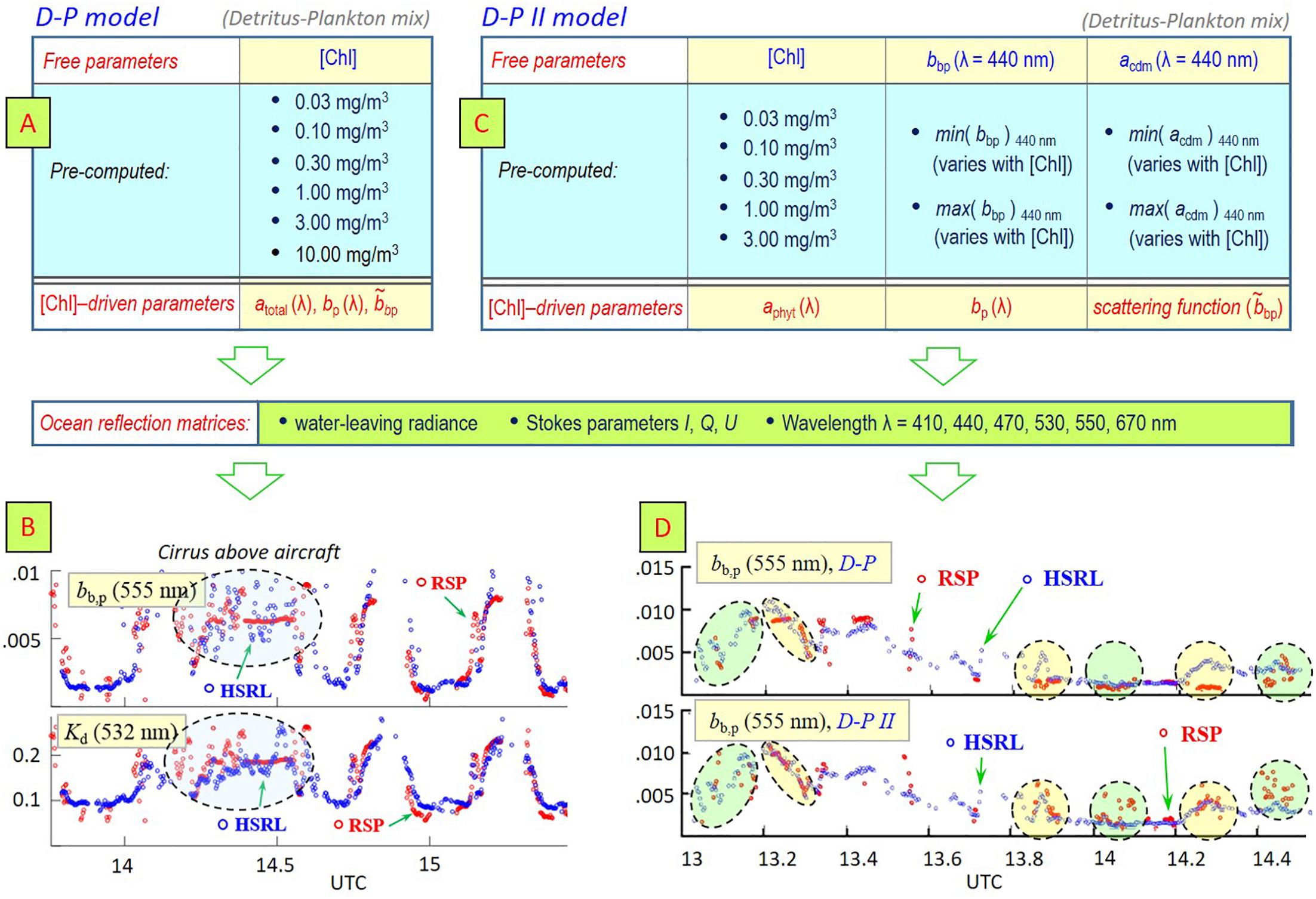
Figure 5. (A) D-P model parameters used for RSP analyses. (B) Comparison for the SABOR campaign between bb,p and Kd values that were retrieved from analyses of HSRL data and from analyses of RSP data using the D-P model. The scatter in the blue-shaded area coincides with the occurrence of cirrus clouds above the aircraft. (C) D-P II model parameters used for RSP analyses. (D) Comparison for the NAAMES campaign between bb,p values that were retrieved from analyses of HSRL data and from analyses of RSP data using the D-P model (upper diagram) and the D-P II model (lower diagram). Yellow and green shaded areas correspond to regions of better and worse agreement when using the D-P II model.
where the reference wavelength λ0 is 443 nm, and from Morel and Maritorena (2001).
Subscripts “p,” “ph,” “cdm,” “dm,” and “y” denote particulate, phytoplankton, colored detrital matter, detrital matter, and yellow substance (i.e., CDOM), respectively. For example, adm is the absorption coefficient for detrital matter, i.e., for the sum of phytoplankton and NAP matter.
Chowdhary et al. (2012) follow Siegel et al. (2002) in assigning the same spectral variation to adm(λ) and ay(λ) because of the difficulty to differentiate between these properties in the inversion of ocean color spectra. Furthermore,
The parameterization in Eq. 5 is taken from Bricaud et al. (1995), with constants A(λ) and B(λ) tabulated by Bricaud et al. (1998, 1999). Note that these constants cover only the spectrum between 400 ≤ λ ≤ 700 nm. The free parameters (i.e., eigenvalues) for the D-P II model are the backscattering coefficient bb,p at λ0 in Eq. 1; the Chlorophyll a concentration [Chla] in Eq. 2; and the absorption coefficient acdm at λ0 = 443 nm in Eq. 3. The prescribed and [Chla]-driven parameters (i.e., eigenvectors) for this hydrosol model are the power law exponent k in Eq. 1, the specific phytoplankton absorption coefficient âph (λ) in Eq. 2, and the spectral decay constant αcdm for absorption by non-algae and dissolved matter in Eq. 3.
The set of parameterizations chosen for bb,p(λ), aph(λ), and acdm(λ) is close to the default configuration (DC) used for the generalized inherent optical properties (GIOP) software database that was developed by Werdell et al. (2013a). The exception is the [Chla]-driven exponent k for bb,p in Eq. 1, which is taken from Morel and Maritorena (2001) instead of retrieving it from water-leaving radiance measurements as in Lee et al. (2002). The D-P II model further adopts the same value of 0.018 nm−1 for αcdm in Eq. 3 as was done for the GIOP-DC database. The RT quantities ω and for the D-P II model are computed in the same manner as for the D-P model (Chowdhary et al., 2006, 2012) except for (1) choosing Eqs 1–6 for the non-water absorption and scattering coefficients, and (2) using the ratio bb,p/ from Eq. 1 for the particulate scattering coefficient bp.
To deploy the D-P II hydrosol model for analyses of air- and spaceborne polarimetric observations over oceans, rigorous underwater light computations were performed with the adding RT method to obtain reflection matrices of diffuse water-leaving radiance (that is, radiance that excludes the contribution of skylight reflected off the ocean surface alone). The ocean reflection matrices were computed only for Stokes parameters I, Q, and U (as defined in Hansen and Travis, 1974) that are measured by existing airborne multi-spectral, multi-angle polarimeters such as RSP (Cairns et al., 1999, 2003), airMSPI (Diner et al., 2013), HARP (Martins et al., 2014), and SPEX (Rietjens et al., 2015). Six wavelengths (410, 440, 470, 530, 550, and 670 nm), 60 viewing and 60 sun angles (both corresponding to 30 equidistant angles up to 64.8° and 30 Gauss integration points between 0° and 90°) were chosen for these matrices. For each wavelength and angle specification, 5 values were chosen for [Chla] (0.03, 0.1, 0.3, 1.0 and 3.0 mg/m3), and 2 values were chosen for bb,p(λ0) and for acdm(λ0) (corresponding to a lower and an upper limit for each of these parameters). The limits for bb,p(λ0) and acdm(λ0), which are different for each [Chla] value, were determined from the synthetic IOP data sets computed in report #5 by IOCCG (2006). Underwater-light computations were performed using 60 Gauss integration points, and the D-P II scattering matrices were renormalized whenever necessary to conserve energy within 10−6. Finally, each ocean reflection matrix was expanded in a Fourier series [using the supermatrix formalism described by de Haan et al. (1987)]. The terms in these allow the ocean reflection matrices to be obtained for arbitrary sun and viewing azimuth angle. Sixteen terms were used for this expansion to obtain an accuracy of 2 × 10⁻⁶ in reflectance units for the water-leaving radiance just above the ocean surface for all angles and [Chla] considered. This accuracy surpasses the PACE accuracy requirement of 5% (cf. “1.1 The PACE Mission” section) by at least an order of magnitude for all sun and viewing angles, all wavelengths, and all [Chla] values considered. In total, 1,728,000 (3 × 3) ocean reflection Fourier term matrices were produced. The D-P II ocean reflection matrices (as well as the matrices for the original D-P model) are publicly available on https://data.giss.nasa.gov/rad/ocean-matrices/, along with their performance analyses and a user manual.
Extensive numerical performance analyses demonstrated that the ocean color variations computed for the D-P II hydrosol model can reproduce those computed for the original D-P hydrosol model, which ensures consistency and continuity between past and future studies that use these detritus-plankton mixture models. Both the D-P and D-P II ocean reflection matrices are currently applied to analyses of concurrently obtained data by the Research Scanning Polarimeter (RSP) and the High-Spectral Resolution Lidar (HSRL) instruments in 3 field campaigns: the 2012 Two-Column Aerosol Project (TCAP) and the 2014 Ship-Aircraft Bio-Optical Research (SABOR) campaign (Stamnes et al., 2018), and the ongoing North Atlantic Aerosols and Marine Ecosystems Study (NAAMES) campaign. Figure 5B shows for SABOR a comparison between RSP and HSRL retrievals for the atmosphere and ocean. The agreement is surprisingly good (even for the indirect-retrieved diffuse attenuation coefficient Kd) given that the simple (1-parameter) D-P ocean reflection matrices were used for these retrievals. These data will be re-analyzed in the near future using the D-P II ocean reflection matrices. The same comparisons are shown in Figure 5D except for the NAAMES campaign using both the D-P (upper row charts) and D-P II (lower charts) ocean reflection matrices. The plankton particulates encountered during this campaign were noted to be unusually small for given [Chla]. This may explain why the RSP retrievals of bb,p sometimes agree less well with the corresponding HSRL measurements (see green-shaded areas) when using the D-P II ocean reflection matrices than when using the D-P ocean reflection matrices. Note that the D-P and D-P II matrices reproduced the same water-leaving radiance for the NAAMES data analyses as evidenced by the retrieval of same aerosol properties (not shown here). Hence, trade-offs appear to be occurring between bb,p and acdm in the D-P II bio-optical model. More analyses of the data collected during NAAMES are currently being conducted to evaluate assumptions made for the IOPs in the D-P II hydrosol model (e.g., the spectral variation of bb,p and acdm in Eqs 1 and 3, respectively).
Another remote sensing algorithm is being developed by a research group led by Peng-Wang Zhai at UMBC, which retrieves aerosols and water leaving radiance simultaneously. Their type (ii) bio-optical model is similar to the formulas outlined by Eqs 1–3, except that the scattering power law exponent k is treated as a retrieval free parameter. In addition, the αcdm value is also treated as a free parameter. INV RT experiments are being performed to test the feasibility of retrieving the power law exponent for particle backscattering fraction. The ocean particulate scattering function are determined by the Founrier-Forand phase function based on backscattering fraction and the Mueller scattering matrix is determined by the measurements by Voss and Fry (1984). These adjustments are designed to accommodate different types of waters in which average laws are not followed. Numerical tests based on synthetic data generated by RT demonstrate that the algorithm can determine aerosol properties and water leaving radiance accurately even for ocean waters with significant sediment concentration (Gao et al., 2018).
The performance of IOP inversion algorithms for PACE-like data will be evaluated by comparing the IOP retrievals with co-located independent IOP measurement sets (cf. “1.1 The PACE Mission” section). However, IOP measurement sets may not always be available for such performance evaluations. In addition, there are always measurement uncertainties which prevent conclusive evaluation of IOP inversion algorithms. To address these cases, the PACE Science Team created a synthetic dataset containing IOPs and remote-sensing reflectance Rrs. The overall scheme follows that adopted by the IOCCG Report 5 (IOCCG-OCAG, 2003; IOCCG, 2006), which was summarized in “Models, parameters, and approaches that are used to generate wide range of absorption and backscattering spectra,” but here the spectral range is expanded (now 350–800 nm), along with wider variations of phytoplankton absorption spectra. Because Hydrolight (Mobley and Sundman, 2013) was used for the generation of Rrs from IOPs, the critical step for this synthetic dataset was the creation of reasonable IOPs spectra for both oceanic and coastal waters. Specifically and briefly, as articulated in IOCCG-OCAG (2003), the absorption (i.e., a) and backscattering (i.e., bb) coefficients, the two key component IOPs for Rrs, were modeled as
Values of aw(λ) were taken from combinations of Lee et al. (2015) (350–550 nm range), Pope and Fry (1997) (555–725 nm range), and Smith and Baker (1981) (730–800 nm range). From more than 4000 measured aph(λ) spectra (spanning 350–800 nm at 5 nm steps), 720 aph(λ) spectra were selected and divided into twelve groups with aph(440) ranging between ∼0.0014 and 39.0 m−1, thus covering oligotrophic oceanic waters to waters with phytoplankton blooms.
Following IOCCG-OCAG (2003), adm and ay were modeled as
where the slope parameters αdm and αy were taken as constrained random values as in IOCCG-OCAG (2003), and adm(440) and ay(440) were modeled as
Parameters p1 ∈ {0.1, 0.6} and p2 ∈ {0.1, 6.0} were constrained random values so reasonable adm(440) and ay(440) values were created for a given aph(440) (IOCCG-OCAG, 2003).
Values of bb,w (λ) were taken from Zhang et al. (2009). Spectra of bb,ph(λ) were also modeled as in IOCCG-OCAG (2003), where bb,ph(λ) is
Here, is the backscattering efficiency of phytoplankton and a value of 1% was taken. Parameters p3 ∈ {0.06, 0.6} and n1 ∈ {−0.1, 2.0} were random values as in IOCCG-OCAG (2003). Similarly, spectra of bb,dm were modeled as
where a value of 1.83% was assigned to the backscattering efficiency for detrital matter, with p4 ∈ {0.06, 0.6} and n2 ∈ {−0.2, 2.2} also random values, respectively.
A number of values for pure (sea)water absorption coefficient aw(λ) have been estimated from laboratory measurements of pure water samples (Pope and Fry, 1997) or modeled using in situ measurements collected from hyper-oligotrophic regions of the ocean (Morel et al., 2007b; Lee et al., 2015). While recent work by Mason et al. (2016) have provided new, high accuracy measurements of pure water absorption in the UV and visible domain, these values are much lower than previously measured in the UV. On the other hand, Lee et al. (2015) have derived values for seawater in the UV that are significantly higher, which may be the result of UV absorption by dissolved inorganic constituents in seawater. Note that the Lee et al. (2015) coefficients were derived from optimizing a remote sensing reflectance inversion model instead of direct experimental measurement of water samples. The aw values of Lee et al. (2015) and Mason et al. (2016) differ by several factors in the UV. The corresponding difference in water-leaving radiance (which is proportional to the inverse of total absorption a in Eq. 7) can for clear waters be much larger than the PACE retrieval requirements (“1.1 The PACE Mission” section). Hence, there is a clear need for research to better understand the role of absorption by dissolved inorganics in the UV such as oxygen, NO3, Br−, and other salt ions comprising sea salts that have significant absorption in the UV (Armstrong and Boalch, 1961; Ogura and Hanya, 1966; Johnson and Coletti, 2002; as cited in Lenoble, 1956; Copin-Montegut et al., 1971; Shifrin, 1988). These effects have received scarce attention in recent literature. At 230 nm, these constituents all have more than an order of magnitude higher absorption than the values of pure water absorption, with steeply increasing absorption at shorter UV wavelengths. An unresolved question is how much these constituents may absorb at wavelengths longer than 300 nm, as the tail absorption effects have typically not been studied with the required accuracy. Even relatively small contributions could be significant since pure water absorption is very low, particularly in the 320 to 420 nm range (<∼0.005 m−1). Armstrong and Boalch (1961) found significant effects of sea salt absorption out to 400 nm, but rigorous purification steps were not taken, so it is unclear if their additions of artificial sea salts introduced organic contaminants.
In addition, the vibrational states and thermodynamic properties of seawater, and hence its optical properties, vary with changes in temperature (T) and/or salinity (S) in various regions of their spectra. Backscattering by pure seawater was often considered a “constant” and “well known” in remote sensing algorithms (e.g., Carder et al., 1999; Lee et al., 2002; Stramski et al., 2004; Twardowski et al., 2005; Werdell et al., 2013a), where common practice for several decades was to use a constant pure seawater backscattering spectra originating from Morel (1974). Note however, in the vast, clear oceanic waters, backscattering by pure seawater can contribute up to 90% to the total backscatter (Shifrin, 1988; Morel and Gentili, 1991; Twardowski et al., 2007). Therefore, uncertainties of just a few percent in bb,w(λ) (the backscattering coefficient for water) can cause the water-leaving radiance to change by more than the 5% retrieval requirement for PACE (see Section “1.1 The PACE Mission”). This also impacts estimating particulate backscatter bb,p because backscattering by the pure seawater component must be subtracted from direct measurements or algorithm retrievals of total backscatter bb. Accordingly, efforts have been made to measure and model the spectral T and S dependencies of aw(λ) (Pegau et al., 1997; Twardowski et al., 1999; Sullivan et al., 2006; Jonasz and Fournier, 2007; Röttgers et al., 2014) and bb,w(λ) (Morel, 1974; Buiteveld et al., 1994; Zhang et al., 2009). The importance of varying salinity and temperature in the computation of bb,w(λ) has been investigated in Werdell et al. (2013b), and been found to have a noticeable effect on IOP retrieved (e.g., ∼3–10% change in retrieved particulate backscattering coefficient bb,p, 1–6% change in non-algae absorption coefficient acdm, and more importantly removal of a bias). About a decade ago, Zhang and Hu (2009) and Zhang et al. (2009) provided the most accurate theoretical description to date of pure seawater scattering as a function of the physical properties of water with variables of temperature, salinity, and pressure. Satellite observations of sea surface temperature (SST; Kilpatrick et al., 2001) and sea surface salinity (SSS; Lagerloef et al., 2008), as well as climatological values (Reynolds et al., 2002; Antonov et al., 2010), have made it now also possible to include T-S dependent bb,w(λ) within inverse algorithms (Werdell et al., 2013b).
Another parameter that has a significant impact on bb,w is the so-called depolarization ratio for pure seawater. The anisotropic nature of water molecules, which produces fluctuations in molecular orientations, is typically described in terms of the molecular depolarization ratio δm, which by definition is the ratio of horizontally polarized light to vertically polarized light at a scattering angle of 90° (see Table 2). The depolarization ratio values currently used by the optics community come from a single study conducted more than 40 years ago (Farinato and Rowell, 1976). In that work, three values were experimentally derived: δm = 0.051, 0.045, and 0.039, with progressively narrower filter bandwidth for stray light removal. Typically, the lowest one measured, δm = 0.039, is recommended because it was obtained with the least contamination of the stray light. This value is therefore, at this time, the accepted community value (Werdell et al., 2018). Pure water scattering in the blue decreases by more than 10% (which for clear ocean waters surpasses the PACE retrieval requirement for water-leaving radiance) when using δm = 0.039 relative to the δm = 0.09 value used by Morel (1974). The Zhang and Hu (2009) computations of pure water scattering with this value of 0.039 produces volume scattering functions that match experimental measurements by Morel (1968) within 2%. Nonetheless, this important parameter deserves additional experimental evaluation to further reduce uncertainties in pure water scattering values. Very recently, Zhang et al. (2019) measured, δm of pure water and seawater at various salinities. They obtained δm = 0.039±0.001 for pure water, which supports the currently adopted value of 0.039. They also found the value of depolarization ratio increases slightly with salinity, by 10–20% at a salinity of 40 g/kg.
Inelastic radiative processes in ocean waters include Raman scattering by liquid water, fluorescence by colored dissolved organic matter (FDOM), and chlorophyll fluorescence. In what follows, we will use inelastic scattering to denote (any of) these processes. Raman scattering is mainly due to the OH bond stretch mode of water molecules (Walrafen, 1967), which absorbs light energy at higher frequency and reemit to lower frequency regions with fixed frequency shift spectra centered around 3400 cm−1. It has been long recognized that the contribution of Raman scattering to the underwater radiation field is significant in the visible region for clear waters (Ge et al., 1995). Chlorophyll fluorescence and FDOM contributes to the water leaving radiance in variable amount depending on wavelengths and water turbidity (Preisendorfer and Mobley, 1988; Green and Blough, 1994). Raman scattering and chlorophyll fluorescence have also been used to better invert the oceanic remote sensing signal to biogeochemical parameters (Behrenfeld et al., 2009; Westberry et al., 2013).
The theoretical modeling of Raman scattering in ocean waters is mostly based on the Monte Carlo (MC) method (Kattawar and Xu, 1992; Gordon, 1999). Kattawar and Xu (1994) have included polarization in the simulation of Raman scattering, in which the radiance was averaged in bins of 30° of azimuth viewing angles to reduce statistical noise. Hydrolight, a commercial software based on the invariant embedding method, can simulate Raman scattering and fluorescence without considering the impacts of polarization (Mobley et al., 2002). Schroeder et al. (2003) have incorporated inelastic scattering in scalar RT models. Semianalytical models have also been developed for under-water reflectance to include Raman effects (Lee et al., 1994; Loisel and Stramski, 2000).
As part of the PACE Science Team effort, Zhai et al. (2015) have implemented Raman scattering in the polarized RT code for atmosphere and ocean coupled systems based on the Successive Order of Scattering (SOS) method. Polarization due to Raman scattering has been preserved and the contribution of Raman scattering to the polarized water leaving radiance has been studied. The coupling mechanism between atmosphere and ocean are fully accounted for. Later Zhai et al. (2017a) added FDOM and chlorophyll fluorescence in their SOS RT code. Their polarized RT code simulation shows that FDOM contributes to the water radiation field in the broad visible spectral region, while chlorophyll fluorescence is limited in a narrow band centered at 685 nm. This is consistent with previous findings in the literature that were obtained with scalar RT codes. With the new polarized RT code, the impacts of fluorescence to the DoLP and orientation of the polarization ellipse (OPE) are studied. The underwater light DoLP is strongly influenced by inelastic scattering at wavelengths with strong inelastic scattering contribution. The OPE for underwater light is less affected by inelastic scattering but it has a noticeable impact, in terms of the angular region of positive polarization, in the backward direction. This effect is more apparent for deeper water depth. These results are important for analyses of underwater light DoLP measurements. The polarized RT code has also been used to study the contribution of polarized water leaving signals to the top of atmosphere in the visible spectra for a range of IOPs for open ocean and coastal waters (Zhai et al., 2017b). Below we discuss RT examples for the impact of inelastic scattering on underwater light radiance at zero water depth.
Figures 6A,B show examples of reflectance spectra with both elastic and inelastic scattering mechanisms included. The simulations are for a coupled atmosphere and ocean system, with the atmosphere characterized by a mixture of molecules and aerosols. The results are for a sensor that is located at the top of the ocean (TOO) just below the ocean surface and that is viewing in nadir direction the upwelling underwater light radiance. The aerosol optical depth at 550 nm is 0.15. Major gas absorptions have been included in the simulation, which include absorptions due to ozone, nitrogen dioxide, oxygen, and water vapor. The ocean optical properties are parameterized in terms of Chlorophyll a concentration [Chla]. The left axis of Figure 6A shows the reflectance (see definition in Table 2) with only elastic scattering included. The right axis of Figure 6A shows the total contribution of both elastic and inelastic scattering, which include Raman scattering, CDOM fluorescence, and chlorophyll fluorescence. The quantum yield of chlorophyll fluorescence used is 0.02, i.e., two percent of the absorbed photons are fluoresced. Figure 6B shows the absolute contribution of inelastic scattering as a function of wavelength.
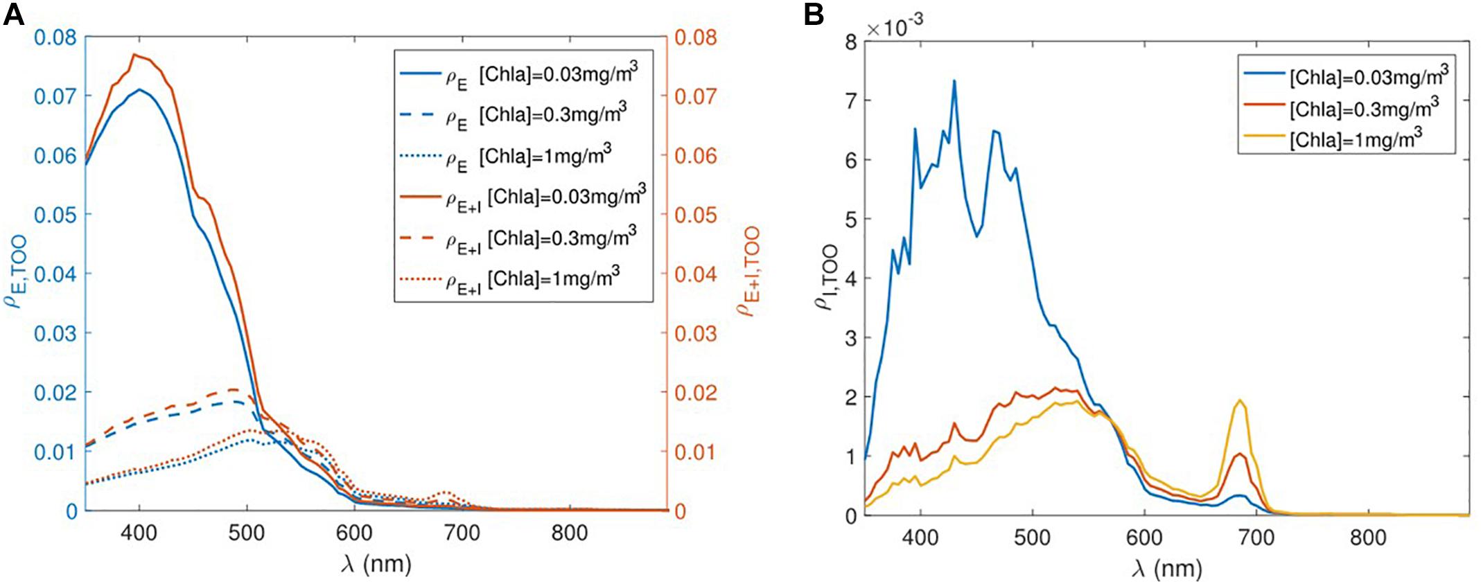
Figure 6. (A) Ocean reflectance at nadir view at the top of the ocean (TOO) as a function of wavelength. (B) The absolute contribution of inelastic scattering to the TOO nadir reflectance as a function of wavelength. Subscripts E and I denote elastic and inelastic scattering, respectively.
Figure 6A shows the spectral behavior of TOO ocean reflectance as a function of [Chla]. There is an anchoring point close to 500 nm where the ocean reflectance is insensitive to the [Chla] values. When the wavelength is smaller than this anchoring point, the ocean reflectance for smaller [Chla] is larger and vice versa for wavelengths longer than the anchoring point. This changes the impact of inelastic scattering on TOO ocean reflectance. For example, ignoring inelastic scattering decreases the TOO radiance in the (deep) blue part of the spectrum by more than 10% if [Chla] becomes small. The corresponding decrease in water-leaving radiance is about 5%, which is equal to the retrieval accuracy requirement for PACE (cf. “1.1 The PACE Mission” section). The opposite trend is seen at 685 nm, where the impact of inelastic scattering causes a peak in TOO ocean reflectance to increase with increasing [Chla]. This peak, which is caused by chlorophyll fluorescence, is more clearly seen in Figure 6B and the corresponding increase in water-leaving radiance surpasses the 5% retrieval accuracy for PACE. Between 400 and 600 nm, the inelastic scattering is still dominated by Raman scattering, whose contribution to TOO ocean reflectance remains large for clearer waters (smaller [Chla] values). These results illustrate the importance of accounting for inelastic scattering processes in polarized RT codes that are used to create synthetic data sets for PACE.
Raman scattering coefficients used in this work are based on measurements (Walrafen, 1967; Hu and Voss, 1997), which do not account for the temperature and salinity dependence. It is understood that the Raman spectra is sensitive to both temperature and salinity (Artlett and Pask, 2015, 2017). In future work, it will be important to systematically parameterize both Raman scattering coefficients and emission spectra in terms of temperature and salinity. For the simulation of FDOM, we have used the excitation – emission spectra from Hawes et al. (1992), which is based on the measurement of FDOM extracted from water samples. Green and Blough (1994) have pointed out that fluorescence is different for FDOM dissolved and extracted from water samples. Further investigation is needed to measure FDOM dissolved in water samples for different geographical and biological origins.
Another important subject on inelastic scattering in FWD RT models is to include non-photochemical quenching (NPQ) in chlorophyll fluorescence (Morrison, 2003). This would create synthetic data sets that allow us to better understand fluorescence signals in satellite observations and to develop more accurate remote sensing algorithm for chlorophyll fluorescence (Behrenfeld et al., 2009). Zhai et al. (2018) have implemented the quenching processes of the phytoplankton fluorescence in their polarized RT code. NPQ modulates the quantum yield of the chlorophyll fluorescence based on the photosynthetically available radiation (PAR), so that the quantum yield is not longer a prescribed parameter. It is a function of both the environmental factors and phytoplankton physiology. Zhai et al. (2018) have simulated the fluorescence for a variety of chlorophyll concentrations, solar zenith angles, and aerosol optical depths. A particularly interesting fact is that the fluorescence is actually higher for larger solar zenith angles or larger aerosol optical depth, which is because the smaller quantum yield due to photochemical and NPQ processes. This has also been observed by geostationary ocean observations (O’Malley et al., 2014)
Over cloud-free oceans, the remotely sensed signal contains contributions from atmospheric scattering, diffuse skylight reflected off the ocean surface, underwater light scattering and direct sun light reflected off the ocean surface (i.e., sunglint). Of all the contributions, sunglint unequivocally provides the brightest and most-recognizable signal: its radiance can exceed the radiance of off-sunglint observations by several factors in the VIS (Ottaviani et al., 2008; Chowdhary et al., 2012) and up to several orders of magnitude in the NIR/SWIR (Chowdhary et al., 2005). To a first order approximation, one can think of sunglint as a mirror-like reflection of the solar beam that is attenuated as light passes though the atmosphere. The extent and magnitude of such pattern depends on the ocean surface characteristics (i.e., wave slope distribution, refractive index), whereas the attenuation by the atmosphere depends on the amount and microphysical properties of aerosols. Remote sensing observations of sunglint can therefore provide information on aerosol properties (Kaufman et al., 2002; Ottaviani et al., 2008, 2013) and on ocean surface slicks when polarimetric measurements are available (Ottaviani et al., 2012). Similar results for oil slick properties were subsequently obtained by Lu et al. (2017) from spaceborne polarimetric observations by the POLDER (Polarization and Directionality of the Earth’s Reflectances) instrument.
It is particularly difficult to retrieve ocean IOPs from spaceborne radiance observations when the scene is contaminated by sunglint. One approach that mitigates this problem is to use the radiance polarized along the meridional plane, which is much less affected by ocean surface reflectance but still provides useful information on ocean color variations (He et al., 2014; Liu et al., 2017). Another approach is to identify (and subsequently avoid) sunglint contaminated scenes by comparing aerosol optical thicknesses retrieved for the same pixel but from different viewing angles. In the latter approach, the sunglint-contaminated retrievals will lead to an identifiable overestimation of the aerosol optical thickness (Harmel and Chami, 2013). The advantage of both these approaches is that they do not require a priori information for the ocean surface roughness; however, they do require the use of multi-angle (and polarimetric) observations. Alternatively, if such observations are not available (e.g., at the edge of the swath monitored by the OCI instrument) then one must resort to ocean surface models to discard sunglint-contaminated scenes based on viewing geometry and surface waviness in space-borne IOP retrievals.
Cox and Munk (1954) were the first to systematically study the relation between the surface slope distribution and the ocean wind speed U12.5 (measured at a height of 12.5 m). Based on airborne photographs of the sun glitter for wind speeds U12.5 ≤ 14 m/s and moderate solar zenith angles, they provided an anisotropic surface slope distribution with a variance depending on the wind speed and wind direction. To a first-order approximation, this surface slope distribution becomes isotropic (Gaussian) with a variance that depends only on the wind speed. Their results have thereafter been adopted by the majority of remote sensing community as a standard model for the ocean surface roughness. Subsequent analyses of passive remote sensing observations from an ocean platform (Su et al., 2002), aircraft (Gatebe et al., 2005) and satellite (Ebuchi and Kizu, 2002; Bréon and Henriot, 2006; Zhang and Wang, 2010) have confirmed the two-dimensional Gaussian surface slope model fitted by Cox and Munk (1954) to a satisfactory/good degree except perhaps for large solar zenith angles. However, variations in the relation between wind speed and the variance of the surface slope distribution were observed. With realistic surface elevations (and hence including realistic surface wave shadowing and multiple reflections) that were obtained from wave variance spectra and Fourier transforms, Preisendorfer and Mobley (1986) and Mobley (2015) used ray tracing techniques to study the reflection and transmission properties of the Cox and Munk surface model with the implicit inclusion of shadowing and multiple reflections. Their studies indicate small difference in surface irradiance reflectance except perhaps for again large solar zenith angles.
When incorporating the Cox and Munk surface model in RT computations to identify sunglint contaminated scenes, there are some aspects to consider. Firstly, to compute the shape and angular extent of the sunglint, one needs wind speed and direction as auxiliary data, which may not always have the appropriate resolution to describe local conditions. Secondly, as mentioned before the relationship between the wind speed (and direction) and the variance of the ocean surface slope distribution can deviate from the relationship given by Cox and Munk (see Kay et al., 2009, and references therein). Thirdly, direct skylight reflected by the ocean surface will still be scattered by molecules and aerosols when propagating through the atmosphere towards the satellite sensor, and this aspect is often ignored when masking the sunglint a priori. For an atmosphere bounded from below by an isotropic rough ocean surface, Ottaviani et al. (2008) found that the error in simulated space-borne radiances may reach 90% (at 470 nm) around the edge of sunglint when ignoring these multiple-scattering effects.
The multiple scattering aspect of sunglint can be expected to be equally important for direct skylight reflected by anisotropic (i.e., wind-direction dependent) rough ocean surfaces. However, while atmospheric attenuation of sunglint reflected by anisotropic surfaces can be incorporated fairly easily in RT methods (Chowdhary et al., 2006; Lin et al., 2016), the inclusion of multiple scattering in the atmosphere of sunglint reflected by such surfaces remains a challenge for most of the RT methods reviewed in Section “2 History of RT Methods for AOS: A Brief Overview.” Masuda (1998) used the adding method to investigate this phenomenon, but he computed only up to three light interactions between the atmosphere and ocean, and he considered only the wavelength of 865 nm. Compared to heritage sensors, the hyperspectral measurements by the OCI and SPEXone instruments onboard the PACE mission will also include shorter wavelengths where light will undergo many more light interactions between the atmosphere and ocean, especially in the blue/UV part of the spectrum. The impact of those interactions on a priori sunglint masks used for aerosol and ocean color retrievals remains uncertain to this date.
At any given viewing geometry, the surface properties determining the ocean surface total reflectance are solely the surface slope distribution and the refractive index m of the ocean-atmosphere interface. Furthermore the surface slope distribution affects the polarized surface reflectance in the same linear proportion as the total surface reflectance, so that the ratio of polarized to total reflectance (i.e., the DoLP) becomes independent of the surface roughness. Hence changes in surface DoLP only occur if the viewing geometry and/or m varies. For remote sensing of cloud-free oceans, this fact was demonstrated by Chowdhary et al. (2005) and Ottaviani et al. (2012), based on RSP observations of DoLP sunglint profiles. Small differences can still occur in airborne observations if the contribution of diffuse light scattered by high aerosol loads within the sunglint region is significant (Ottaviani et al., 2019).
The surface refractive index m varies throughout the global oceans in response to several factors. Firstly, m is determined by the dielectric constant which, for pure seawater and at any wavelength, varies with temperature T and salinity S (Röttgers et al., 2014). Variations in m caused by changes in T are relatively small, i.e., 0.002 in the VIS-NIR if T increases from 0 to 30°C. Similar variations are observed if S increases from 30 to 40 g/kg, a range which covers most of the global oceans except for the Arctic regions. Secondly, substances that cover the ocean surface such as floating seaweed, plastics, and slicks from biogenic origins (e.g., plankton and fish secretions) and anthropogenic origin (e.g., oil spills) affect m depending on the composition and thickness of the floating substance, and on the wavelength of light. For example, a thick oil slick can cause m to increase by 0.1–0.2 in the VIS-NIR depending on the oil type, refinement, wavelength, and temperature (Otremba, 2000; Carnesecchi et al., 2008). Thirdly, the uppermost 1–1000 μm of the ocean – referred to as the surface microlayer (SML) – has biological, chemical, and physical properties that are distinctly different from those of the underlying ocean body (Engel et al., 2017, and references therein). Little is known about the processes controlling the SML properties, yet the SML is a key player in gas exchanges between the atmosphere and ocean, and it is a major source of biogenic matter found in sea-spray aerosols. The high occurrence in the SML of marine gel particles (in addition to colloids, particulate matter, neuston assemblies, and CDOM) gives it a gelatinous nature, which in turn promotes aggregation of particulates and natural colonization of bacteria. Polarization measurements obtained by Kozarac et al. (2005) for in situ and ex situ SML samples show that the complex composition of SML has an impact on the surface m; however, the resulting absolute change in m remains unknown. Regarding the sunglint DoLP variations with m and with viewing geometry: consider for instance light illuminating an ocean surface at an angle θi (measured from the upward surface normal). When θi becomes equal to the Brewster angle θb ≡arctan(m), the specularly reflected light becomes completely polarized (i.e., DoLP becomes 100%: Born and Wolf, 1999). Variations in m cause the angular location θb of maximum DoLP to shift and, as a consequence, the DoLP to change if the incident and viewing angles are kept constant.
Airborne multi-angle observations of the DoLP obtained with the RSP instrument in the SWIR are ideally suited to study variations in m. The penetration depth at SWIR wavelengths is of the order of tenths of a micrometer because of strong absorption by water, i.e., it appropriately targets slicks, films, and SML. In addition, the molecular and aerosol optical thicknesses are very small at these wavelengths, which enlarges the spatial dimension in airborne observations of sunglint-dominated scenes (i.e., of scenes that are least affected by diffuse atmospheric scattering). The multiangular (∼150 views) capability of RSP allows sunglint to be sampled at high spatial resolution in transects flown near the principal plane. Finally, the high accuracy of RSP DoLP measurements (i.e., better than 0.2%) allows to identify changes in sunglint DoLP profiles caused by minuscule variations in m (as small as 1 × 10⁻⁴ under ideal experimental conditions). Using RSP data collected while flying over the Deepwater Horizon oil spill, Ottaviani et al. (2012) reported changes in m by 0.064 at λ = 2.2 μm for oil-affected scenes (cf. Figure 7B, and related discussion below).
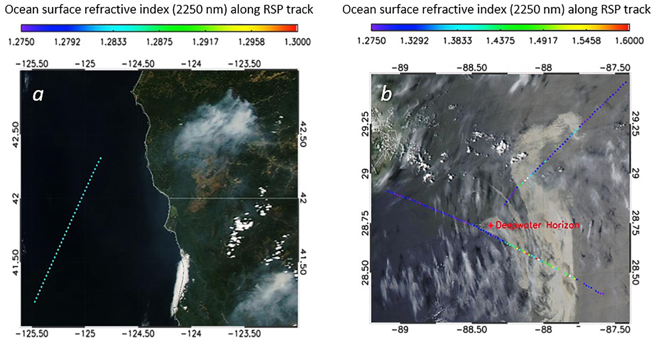
Figure 7. Successful retrievals of the ocean surface refractive index from RSP measurements at 2.2 μm, over near-real-time imagery from the MODIS sensor. (a) SEAC4RS campaign (08/02/2013): test flight over pure seawater. Note that the color bar covers for this panel only a small range of the refractive index. (b) CARES/CalNEX campaign (05/11/2010): transects intersecting the oil spill caused by the explosion of the Deepwater Horizon offshore platform. The refractive index of pure seawater at 2.2 μm measured in laboratory experiments by Segelstein (1981) is 1.2815.
Recently, we exploited a general algorithm based on a Levenberg–Marquardt type of inversion (Rodgers, 2000) to provide continuous retrievals of the refractive index along RSP flight transects. Using the average of 20 RSP scans at a time (corresponding to time intervals of ∼15 s), the procedure starts with the identification of the sunglint-dominated views in the DoLP measured at 2.2 μm, achieved by selecting the series of consecutive views for which the DoLP is closest to that predicted by the Cox and Munk relation. The inversion is then launched with the refractive index as the sole free parameter. Even in this simplest version, the algorithm shows remarkable stability and accuracy as demonstrated in Figure 7. The transect in panel (A) belongs to a test flight during the SEAC4RS (Studies of Emissions and Atmospherric Composition, Clouds, and Climate Coupling by Regional Surveys) campaign, when after sampling fires in Southern Oregon, the aircraft veered toward Case I waters off the Southern Oregon/Northern Californian coast. Panel (B) presents two flight legs obtained during the CARES/CalNex (Carbonaceous Aerosols and Radiative Effects Study/California Research at the Nexus of Air Quality and Climate Change) campaign that intersected the oil spill caused by the explosion of the Deepwater Horizon oil rig in 2010. For both these campaigns, where the RSP flew at two very different altitudes (∼20 km on an ER-2 aircraft during SEAC4RS, and ∼9 km on a B-200 aircraft during CARES/CalNex) and under very different atmospheric conditions, the algorithm retrieves very plausible refractive indices with high accuracy. In particular, note the small variability of the refractive index in panel (A), where the average over the whole leg is 1.2836 with a standard deviation of 0.0007. This result is particularly interesting in view of the possible detection of floating layers of biogenic materials. We further speculate that the temperature and salinity dependence of the refractive index can be observed in case of large gradients such as river waters flowing into oceans. The method also offers an alternative to measurements otherwise difficult to obtain, as is the case for the determination of the refractive index of oil (Ottaviani et al., 2012). Ottaviani et al. (2019) extended this method to a complete series of RSP transects, including a thorough assessment of the sensitivity to the residual aerosol effects and the inclusion of additional free parameters during the inversion.
The lessons learned from these RSP inversions will aid the interpretation of DoLP data obtained by PACE (see Section “1.1 The PACE Mission”) in sunglint regions. However, PACE polarimetry will occur at shorter wavelengths (i.e., in the NIR) than those of RSP. This means that aerosol scattering contributions may not be negligibly small. Furthermore, PACE polarimetry will occur at fewer viewing angles (i.e., ≤10), and at least for HARP2 at coarser DoLP accuracy (i.e., ≤1%). These reductions in measurement capabilities lead to a decrease in the retrieval accuracy of surface refractive indices from sunglint DoLP data, even in absence of aerosol scattering. Nevertheless, DoLP measurements of sunglint that were obtained by POLDER at a coarser accuracy (∼1%) in the NIR (870 nm) for ≤ 14 viewing angles have still proven useful in distinguishing between surface refractive indices retrieved for clean ocean waters and for oilslick covers (Lu et al., 2017). Hence, while PACE DoLP measurements of sunglint will not lead to the same retrieval accuracies for surface refractive index as RSP, they will likely contain information that can be used to not only detect and but also identify substances covering large sections of the ocean surface. This remains a research topic for the near future.
Early quantitative work on oceanic whitecaps was initiated by Monahan (1971), who studied photographs of ocean surface in order to derive the spatial fraction fwc of area covered by whitecaps. His results, which were obtained for wind speeds at 10 m above the sea surface, U10, smaller than 10 m s−1, set forth the functional form fwc ∼(U10) k where k is a constant. Wu (1979) argued on physical grounds that the exponent k should be 3.75, and fitted Monahan’s (1971) results and other data to fwc = 1.7 × 10⁻⁶ U103.75. The same data sets were used by Monahan and O’Muircheartaigh (1980) to statistically analyze seven solutions for fwc ∼ (U10) k proposed in the literature. They found Wu’s (1979) expression to result in one of the best fits, and a linear regression analyses performed by these authors revealed an expression with only slightly smaller errors. Note, the scatter in the data from which to fwc was retrieved is very large, i.e., of the order of fwc itself. For many RT applications, it has been customary to adopt their expression of fwc = 2.95 × 10⁻⁶ U103.75, as a standard for the following decades. For remote sensing applications, other relationships have been used. Ocean color satellites currently employ an expression derived by Stramska and Petelski (2003) for undeveloped seas where fwc = 8.75 × 10⁻⁵ (U10-6.33)3. At high wind speeds, however, a threshold equivalent to the whitecap fraction at 12 m s−1 is implemented in the operational code (see atmospheric correction section). Newer measurements of whitecaps under high wind situations in the polar seas suggest that fwc does not follow a cubic relationship at high wind speeds fwc = 7.38 × 10⁻⁴(U10-4.23)1.42 (Brumer et al., 2017).
The whitecap albedo Awc has also been the subject of various research. Whitlock et al. (1982), who studied laboratory-generated whitecap patches, found that the reflectance of whitecap varies significantly at wavelengths larger than 0.9 μm, but that it remains fairly constant at smaller wavelengths with Awc ≈ 50% for freshly generated thick whitecap and Awc ≈ 10% for a single bubble layer. Koepke (1984), who studied time-resolved pictures of whitecaps through a red filter, observed on the other hand that the reflectance of oceanic white caps decreased rapidly as they age. By averaging over time and setting limits to the whitecap reflectance based on the Whitlock measurements, he derived an effective white cap albedo of 22% ± 8%. Frouin et al. (1996) studied whitecap reflectance created by breaking waves, found that it decreased by 40–85% as the wavelength increased from 0.85 to 1.65 μm. They explained this spectral behavior by considering the nature of oceanic whitecap – i.e., air bubbles separated by a thin layer of water (surface foam), and bubbles injected into the upper layer of the ocean body. The spectral decrease in whitecap albedo Awc could then qualitatively be described by the increase in absorption by water between the air bubbles. A similar spectral dependence of Awc was also observed by Moore et al. (1998), who monitored whitecaps generated in the open ocean by the bow of a moving ship.
The relationship between whitecaps and liquid water absorption implies that these can be tied within the theoretical framework of RT modeling. Whitecaps belong to a broad class of strongly multiple-scattering media where the volumetric concentration of bubbles is greater than 70% (Kokhanovsky, 2004). RT modeling typically applies to media with low concentrations of scatterers (<1% by volume), but progress has been made in the development of RT theory of whitecaps (Kokhanovsky, 2004; Ma et al., 2015). However, more research is needed to validate the theoretical models with experimental measurements.
The PACE mission aims to be hyperspectral from the UV into the NIR wavelengths and will require a more spectrally resolved whitecap reflectance. New spectral measurements of whitecap have been made across from 400 to 2500 nm (Figure 8). These measurements show that whitecaps are not featureless in the NIR but have dips in reflectance that largely correspond to the absorption features of liquid water. Reflectance dips occur particularly at 750, 980, and 1150 nm, which have enhanced liquid water absorption, a result of multiple scattering in and around the subsurface bubbles and surface foam (Dierssen, 2019). Following Whitlock et al. (1982), a simple model of whitecap reflectance based on the natural logarithm of water absorption can be used to describe the spectral shape of intense whitecaps generated by breaking waves into SWIR wavelengths (Dierssen, 2019). Moreover, the decrease in reflectance at these liquid water absorption bands is correlated with enhancements in reflectance of the whitecap across the spectrum. Dierssen (2019) found that more intense whitecap causes enhanced absorption by liquid water, likely as a result of enhanced multiple scattering within the surface foam and submerged bubbles, that is correlated with the reflectance of the whitecap feature.
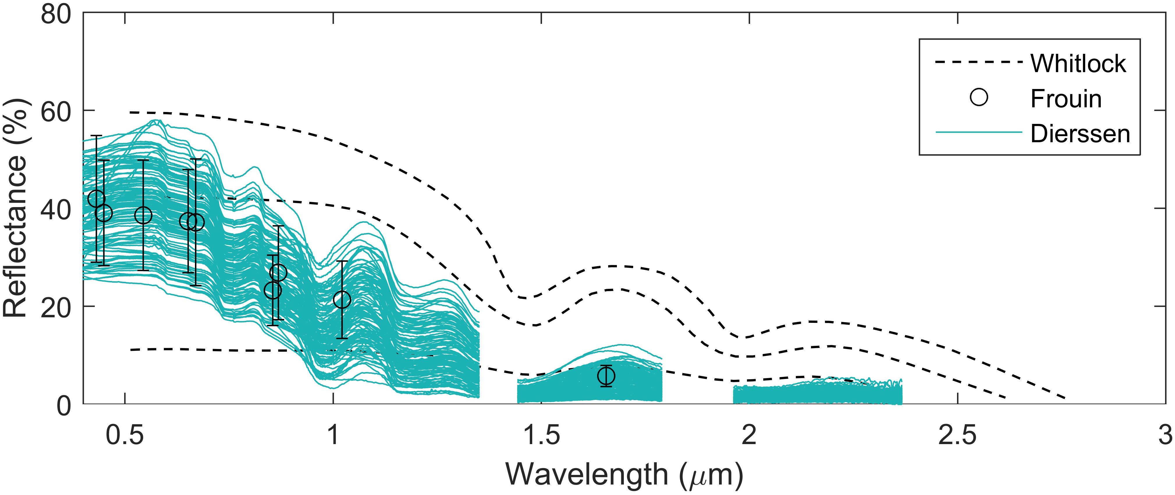
Figure 8. Spectral reflectance of the whitecap of breaking waves measured from visible to short-wave infrared with black dashed lines from Whitlock et al. (1982, Figure 2a) and circles with error bars from Frouin et al. (1996). The different black-dashed lines correspond to different foam samples, with upper and lower curves corresponding to clear water foam patches with multiple- and single-bubble layer, respectively. Cyan lines are new hyperspectral measurements of breaking waves from Dierssen (2019) as part of the PACE project showing the liquid water absorption features at 0.750, 0.980, and 1.150 μm. The gaps in the measured spectrum correspond to regions where the atmosphere is opaque and downwelling irradiance is too low for a reliable signal.
Current FWD RT models based on wind speed and a single whitecap albedo cannot be used to accurately represent the diversity of whitecaps on the ocean. The manifestation of whitecaps and the amount of sea surface covered by surface foam and submerged bubbles are influenced by a variety of other factors including fetch and duration and the wind, water temperature, air temperature and stability of the lower atmosphere defined by the air/water temperature differential, salinity, current shear and long wave interaction, wave age, and the presence of surfactants such as organic films (e.g., Brumer et al., 2017). Furthermore, RT models should transition from using a single albedo to a more realistic framework that incorporates reflectance from actively breaking waves and residual bubble plumes and potential changes in albedo relating to the condition of the seas (Randolph et al., 2014, 2017; Xu et al., 2015). Potentially new RT models for estimating the contribution of whitecaps on the sea surface are presented in Dierssen (2019), including an effective whitecap factor that is based on optical reflectance rather than the traditional interpretation of whitecap fraction as an aerial average of bright features. Improving estimates of whitecap reflectance under high wind conditions will also improve the retrievals of aerosols, since presently the enhanced reflectance is incorrectly removed in the aerosol algorithms. The spectral aerosols models are not identical to whitecap reflectance and hence errors will be propagated from the NIR/SWIR to visible wavelengths under high wind conditions. Image-based retrievals of whitecap reflectance, rather than use of a windspeed climatology, should improve the PACE overall accuracy of retrievals of both oceanic and atmospheric constituents, particularly in high wind areas like the Southern Ocean.
With the addition of polarization capabilities on the PACE mission, future research is also warranted on the polarization effect of wind-roughened seas and whitecaps. Polarized reflectance has been considered for whitecap-free waters covered by ocean waves of various heights and periods, including wave shadowing at high incident angles (Mobley, 2015; Hieronymi, 2016). However, little research has been done on the polarization of light reflected by whitecaps. That is, surface foam is commonly modeled as a Lambertian reflector (Koepke, 1984; Gordon and Wang, 1994a) which renders unpolarized light. However, light scattered by a single submerged air bubble is highly polarized (akin to Raleigh scattering) because of a refractive index smaller than one relative to water (Mishchenko et al., 2002). Multiple scattering by a cloud of bubbles that make up whitecaps reduces the polarization, which is qualitatively consistent with analyses of CALIPSO (Cloud-Aerosol Lidar and Infrared Pathfinder Satellite Observation) data (Hu et al., 2008). However, there exist no model computations to provide quantitative corroborations. Hence this remains an important outstanding topic for future research.
Aerosols originate from a wide range of sources including wind processes (Prospero et al., 2002; Carslaw et al., 2010; Burrows et al., 2014; Quinn et al., 2014), volcanic (Toohey et al., 2016) and biogenic emissions, combustion of fossil fuel and biomass (van der Werf et al., 2010; Lamarque et al., 2010; Bauer et al., 2016), and chemical processing of gaseous precursors. Once in the atmosphere particle properties can change during transport through such processes as hydration, evaporation, aging, chemical reactions, and coagulation (Ghan and Schwartz, 2007; Baker et al., 2014). Finally, aerosols are removed from the atmosphere by wet (in-cloud processing and rain) and dry (sedimentation and coagulation) deposition processes, which, in addition to environmental circumstances, depend on the particle physical and chemical properties (Bergametti and Forêt, 2014). The result of these multiple sources is to create a wide variety of aerosol types whose physical and optical properties vary widely with space and time.
Only space-borne observations can provide a global overview of the variability of aerosol properties. Remote sensing of aerosols from space requires accurate RT modeling of the atmosphere with aerosols properly represented in the model. The RT characteristics of aerosols that affect the reflected light measured by satellite sensors are their single scattering albedo ω, optical thickness τ, and scattering function F (or 4 × 4 scattering matrix F when accounting for the polarization of light). In the simplest case (i.e., single scattering by one aerosol type), the radiance emerging from the top of the atmosphere (TOA) becomes proportional to the product of these three RT quantities. Early studies showed that the linear relationship between the TOA radiance and τ can be preserved for multiple scattering (Griggs, 1983), and this formed the foundation for the first aerosol retrievals of τ from various satellite observations including AVHRR (Advanced Very High Resolution Radiometer) data (see Griggs, 1984). However, the radiances used for these retrievals were all measured at a single wavelength (centered close to 0.65 μm) and at a single viewing angle, i.e., they provided only a single data point from which only one aerosol RT quantity could be retrieved. Hence retrieving τ from these radiance measurements required that ω and F had to be assumed a priori, which is difficult given the large spatial and temporal variations in aerosol properties discussed above. Note that, even for the simplest case (i.e., one aerosol type consisting of homogeneous spherically shaped particles), ω and F in turn depend on 4 particle properties: the real and imaginary part of the refractive index m, and the effective radius re and effective variance ve of the size distribution n(r) [note from Hansen and Travis (1974), that re and ve are not very sensitive to the shape of n(r)] – all of which are effectively assumed in AVHRR retrievals (Rao et al., 1989; Stowe et al., 1997). Higurashi and Nakajima (1999) reduced the assumption requirements by including the radiance measured at a second AVHRR channel (centered at 0.83 μm) to retrieve a measure for the size distribution (i.e., the Ångström exponent). However, the complex refractive index still needs to be assumed for such cases. Analyses performed by Mishchenko et al. (1999) show that erroneous assumptions made for the complex refractive index will significantly affect the τ values retrieved from AVHRR observations.
The need for more pieces of information measured by space-borne sensors was addressed by observations from a new generation of satellite instruments that were launched in succession (Kaufman et al., 1997), including those that are part of NASA’s Earth Observing System (EOS) program. Specifically, the MODIS (Moderate Resolution Imaging Spectroradiometer) instrument onboard the Terra platform (launched in 1999) and Aqua platform (launched in 2002) provides radiance measurements in more wavelength bands that cover a larger spectrum than the AVHRR instrument (Barnes et al., 1998). Six of those bands, covering the spectrum 0.55–2.13 μm, are used to retrieve aerosol properties over ocean (Tanré et al., 1997; Levy et al., 2013). On the other hand, the MISR (Multi-angle Imaging Spectroradiometer) instrument onboard the Terra platform provides radiance measurements in nine viewing angles that cover a satellite viewing angle range of ± 70.5 Diner et al., 1998). The measurements in all nine directions are made in four wavelength bands, two of which (centered around 0.672 and 0.867 μm) are used for the standard aerosol retrieval over ocean (Martonchik et al., 1998; Kahn et al., 2001). Observations provided by the MODIS and MISR instruments have created to this date a wealth of new information on aerosol variability. Still, assumptions continue to be made about the RT properties of aerosol species, mainly derived from surface measurements and ground-based remote sensing retrievals. While considerable effort has been placed into matching these assumed particle properties to laboratory and field data, by definition they cannot replicate the full range of continuous temporal and spatial changes in ambient aerosol properties that is occurring in our Earth’s atmosphere. Even if one were to adopt more elaborate retrieval algorithms such as GRASP (Generalized Retrieval of Aerosol and Surface Properties) (Dubovik et al., 2011, 2014) which does not rely on pre-defined discrete aerosol species, theoretical studies show (e.g., Knobelspiesse et al., 2012) that MODIS-like and MISR-like observations do not contain enough information to adequately capture (as defined in Mishchenko et al., 2004) these changes in ambient aerosol properties.
To improve the aerosol properties retrieved from instruments like the MODIS and MISR instruments, one must consider extending the spectral range monitored by these instruments and/or include measurements of the polarization of light. For example, the UV radiance provides more useful information on aerosol absorption than the VIS-SWIR radiance because of the rapid growth (∼λ−4) of the molecular optical depth with decreasing wavelength λ, which causes a substantial increase in multiply scattered (and hence in multiply absorbed) light. Torres et al. (2005, 2007) and Satheesh et al. (2009) demonstrated this capability from analyses of space-borne observations in the near UV by the TOMS (Total Ozone Mapping Spectrometer) and OMI (Ozone Monitoring Instrument) instruments in the near-UV. The caveat in making practical use of the enhanced aerosol absorption in the near UV is that strong vertical variation in molecular scattering in the atmosphere introduces ambiguities in standard retrieval algorithms. Coupling between molecular scattering and aerosol absorption varies with the relative concentration of molecules and aerosols, which in turn is dependent on their vertical distribution. Thus, in practical terms a range of aerosol layer height/ absorption/optical thickness can produce the same measured radiance in the near UV. To unambiguously retrieve aerosol absorption properties, either layer height or aerosol optical depth must be constrained. Heritage studies approach this ambiguity by assuming layer height, usually through model output or climatology (Torres et al., 2005, 2007) or by introducing simultaneous observations at longer wavelengths that can be extrapolated to the UV wavelengths to constrain aerosol optical thickness (Satheesh et al., 2009; Gassó and Torres, 2016).
Even more promising, the linearly polarized radiance scattered by aerosol particles provides more information about the microphysical and chemical properties of these particles than their scattered radiance does. That is because (Hansen and Travis, 1974; Mishchenko and Travis, 1997):
i Radiance is described by just one measurable quantity, i.e., the Stokes parameter I, whereas linearly polarized radiance is described by two measurable quantities, i.e., (see also Table 2) the Stokes parameters Q and U (or, equivalently, the DoLP and the polarization angle χ);
ii The single-scattering angular features in Q and U are sharper, more numerous, and show larger sensitivity to variations in aerosol size distribution and complex refractive index than the corresponding single-scattering angular features in I;
iii The single-scattering angular features in Q and U are much better preserved in the presence of multiply scattered light than the corresponding features in I;
iv When I, Q, and U are measured simultaneously then the uncertainty in DoLP becomes independent of (and hence in degradations of) the absolute calibration uncertainty.
If the remaining uncertainty in DoLP is kept below 0.5%, then one can use multi-angle, multi-spectral measurements of I, Q, and U to retrieve aerosol properties (in real time, using no pre-defined aerosol models) with sufficient accuracies that meet the criteria for climate change studies. This has been demonstrated in numerous theoretical studies (Mishchenko and Travis, 1997; Hasekamp and Landgraf, 2005, 2007; Knobelspiesse et al., 2012), and is supported by analyses of actual, airborne, multi-angle, multi-spectral polarization measurements (Chowdhary et al., 2001, 2002, 2005, 2012; Wu et al., 2015, 2016; Xu et al., 2016). Of particular interest in these analyses are the first-in-kind retrievals of the spectral complex refractive index, which is a measure of aerosol composition. Spaceborne multi-angle, multi-spectral, multi-Stokes-parameter (3M) radiance measurements have been provided since 1996 in intermittent intervals by the POLDER-1, POLDER-2 and POLDER-3 instruments (Fougnie et al., 2007), but the DoLP uncertainty is larger than 0.5% (commonly assumed to be 1%) for these instruments (Knobelspiesse et al., 2012). Nevertheless, analyses of their measurements have produced new results for the optical properties of liquid clouds (e.g., Bréon and Goloub, 1998; Riedi et al., 2000; Bréon and Doutriaux-Boucher, 2005; Shang et al., 2015) and ice clouds (Chepfer et al., 2001; Baran and Labonnote, 2006; van Diedenhoven et al., 2014), of aerosols over cloud-free oceans (e.g., Tanré et al., 2001, 2011; Bellouin et al., 2003; Herman et al., 2005), and of aerosols above clouds (e.g., Waquet et al., 2013a,b; Peers et al., 2015) and in between clouds (van der Stap et al., 2015).
The prospect of using highly accurate 3M radiance and/or (hyperspectral) UV-SWIR radiance measurements to retrieve aerosol optical and physical properties also poses new challenges for the interpretation of these retrievals. For example, the majority of existing retrieval algorithms such as GRASP still assume a single complex refractive index for the fine mode aerosol, and a single complex refractive index for the coarse mode aerosol. In reality, each aerosol mode may consist of several components that are either internally or externally mixed. The challenge here is to extract those individual components from the retrieved m, ω, re, ve, τ and particle shape. Internal mixtures come in many varieties that may involve both soluble and (non-spherical) insoluble components (Gibson et al., 2007; Wise et al., 2007; Freney et al., 2010). For such mixtures one may, under certain circumstances (Mishchenko et al., 2016), use the Maxwell Garnett effective medium approximation (Bohren and Huffman, 1983) to decompose the retrieved effective m into those of the individual components. Schuster et al. (2016) adopted such an approach (albeit for the spectral variation of the retrieved ω) to extract the relative proportion of carbonaceous aerosols and free iron minerals (hematite and goethite) in absorbing aerosols. Alternatively, one may use brute force, state-of-the-art RT methods to study (and possibly characterize) the scattering patterns of internally mixed complex components (Mishchenko and Dlugach, 2012; Mishchenko et al., 2013; Li and Mishchenko, 2016). The case for externally mixed components is more challenging, as there are no simple rules for the effective m and ω for such mixtures. Hasekamp et al. (2011) and Russell et al. (2014) use a particle volume-weighted approach to obtain an effective refractive index for an external mixture of a fine and a coarse mode aerosol. However, the validity and limits of this approach remain to be investigated for external mixtures. Alternatively, one may just simply want to flag the presence of externally mixed multiple aerosol types. The multi-parameter classification method described by Russell et al. (2014) for a dominating single aerosol type offers a possible venue for such tasks. Regardless of the aerosol mixture type, identifying the individual components will require an extensive database of their complex refractive indices that covers the full spectral range of UV-SWIR.
The PACE mission will continue to need well-defined characterization of aerosol optical properties for RT calculations, but will require those models to cover the expanded spectral range and spectral density of OCI. As explained above, even algorithms applied to a PACE polarimeter measuring 3M will require advanced (e.g., multi-component, inhomogeneous) aerosol models to test the remaining assumptions inherent in those algorithms. Thus, aerosol models for RT in the PACE era will need to be even more detailed, with greater characterization and better accuracy than they are now. These requirements and considerations apply across the board to the next generation of sensors intending to enhance aerosol characterization from space, not just to the three PACE instruments. For example the multi-viewing multi-channel multi-polarization imager (3MI) (Fougnie et al., 2018) will face the same challenges in validating retrievals and supporting remaining assumptions as the PACE polarimeters, and will require comprehensive measurement-based aerosol models.
Through the era of the Earth Observing System (EOS) that began with the launch of the Terra satellite, aerosol models for RT and remote sensing have become anchored in the statistics from the aerosol properties retrieved from the ground-based remote sensing measurements of the Aerosol Robotic Network (AERONET; Holben et al., 1998; Dubovik and King, 2000; Dubovik et al., 2000). The AERONET database provides a wealth of statistics of retrieved aerosol optical properties that cover a wide range of conditions, although the open ocean is not well sampled. This allows linking variability in optical properties to measurable or retrievable parameters, such as aerosol optical depth, or more recently to relative humidity (Ahmad et al., 2010). Furthermore, representations of aerosols in RT are moving away from assumptions of sphericity and Mie theory (Meng et al., 2010; Gassó and Torres, 2016; Lee et al., 2017).
However, remote sensing inversions from AERONET are inadequate by themselves to provide all the detailed characterization necessary for the PACE era. For example, the four discrete measured and inverted wavelengths from AERONET do not span the spectral range and resolution needed by PACE, and specifically do not include any characterization of the UV. The SkyNet network provides an alternative, though less widely distributed network of upward-looking radiometers and inversion products that include measurements and inversions at UV channels (Takamura and Nakajima, 2004), which will help, but again will not be adequate by themselves. Another example is the lack of models in AERONET inversion methods that properly characterize important aerosol types such as volcanic ash and biogenic particles. To obtain the necessary aerosol characterization from PACE we will require measurements made in situ, either in the laboratory or in the field. These should include spectral absorption/single scattering albedo and real part of the refractive index across the spectrum measured by PACE OCI and especially in the near-UV, particle size, and spectral elements of the scattering phase matrix including single scattering phase function/polarized single scattering phase function (Kahn et al., 2017). Then, to make use of these measurements for RT and remote sensing in the atmosphere, we need a set of complementary measurements to translate the in situ measurements to ambient conditions in the atmospheric column. These ancillary measurements should include aerosol layer height, particle hygroscopicity growth factor, among others, depending on the measurement situation (Kahn et al., 2017).
In addition, we foresee that new scrutiny of the FWD RT problem may be needed. Tolerable accuracy for analyses of past and current aerosol satellite sensors may no longer be sufficient to match PACE’s accuracy requirements for hyperspectral radiometry and multi-angle polarimetry in the UV-VIS. To this end, we need benchmarking of RT codes for coupled AOS models that, in addition to hydrosol particulates (cf. “3.4.1 RT Validations” section), also include aerosol scenarios. It will also be necessary to re-evaluate modeled molecular scattering profiles that are important for the interpretation and retrieval of aerosols from measurements in the near-UV. Inclusion of inelastic atmospheric processes in atmospheric models has already begun (see e.g., Landgraf et al., 2004; Deelen et al., 2005; Spurr et al., 2008; Rozanov et al., 2014, 2017; Lelli et al., 2017). The point is that as space-based measurements improve and add capability for aerosol characterization, aspects of RT code that introduce uncertainties too small to affect simplistic aerosol retrievals may now create too much uncertainty to make use of the new measurements. Even the input solar spectrum becomes a source of unacceptable error, again in the near-UV where uncertainties in solar spectrum measurements are worse (see also discussion in Section “3.4.3 UV Remote Sensing of AOS”). Finally, optimal estimation methods used to make use of the information data set provided by multi-angle polarimeters require on-line RT calculations, rather than Look-Up Tables. This requirement makes real-time aerosol retrievals cumbersome in an operational environment. Speeding up RT codes, without losing accuracy, will be a high priority.
Laboratory and field measurements are beginning to meet the challenge of providing aerosol characterization with greater detail and accuracy, and for a wider variety of aerosol types. A new technique (Martins et al., 2009; Rocha-Lima et al., 2014, 2018), that is able to determine spectral absorption/single scattering albedo continuously from 300 to 2500 nm has been applied to volcanic ash and Saharan dust particles (Figure 9), although it is still unclear how to translate these laboratory measurements to ambient atmospheric conditions for RT. Another measurement innovation that can provide greater detail for aerosol models is airborne measurement of particle phase matrix elements (Dolgos and Martins, 2014). By measuring the single scattering function and polarized phase function across the range of scattering angles from 3° to 177° at 1° angular resolution, we can distinguish aerosol type, even separating similar fine mode types such as biogenics and biomass burning (Figure 10; Espinosa et al., 2017). Polarization is necessary to make that distinction and physically the differences lie mainly in differences in real part of the refractive index, not in size of the particles. Then, similar to inversions applied to AERONET observations, inversions applied to these measured phase matrix elements can provide size distribution and real part of the refractive index (Espinosa et al., 2017). The scattering measurements are made in situ from aircraft and are subject to particle size limitations imposed by inlets and loss of volatiles as noted in other in situ measurements, but similar measurements can be made in ambient conditions with a specially designed open-path instrument mounted below the aircraft wing that eliminates the need for inlets or tubes. Direct measurements of scattering matrix elements depend on discrete laser wavelengths that inadequately span the spectral range of future space sensors. However, recently a custom instrument was used with laser wavelengths at 375 nm and 405 nm to characterize phase matrix elements of biomass burning aerosol in the deep blue and near-UV (Manfred et al., 2018), an important step forward toward providing the input to RT modeling in the PACE era. The recent work shown above is just a sample of the increased capability of laboratory and in situ field measurements of aerosol particle properties now reaching a mature stage. As deployment of these new measurement systems increases and the database of particle characterization grows, we can use these detailed measurements to guide the development of new aerosol models for RT that will span OCI’s broad spectrum and represent new aerosol types. The challenge will be in translating these in situ measurements to represent aerosol properties of the total column in ambient conditions.
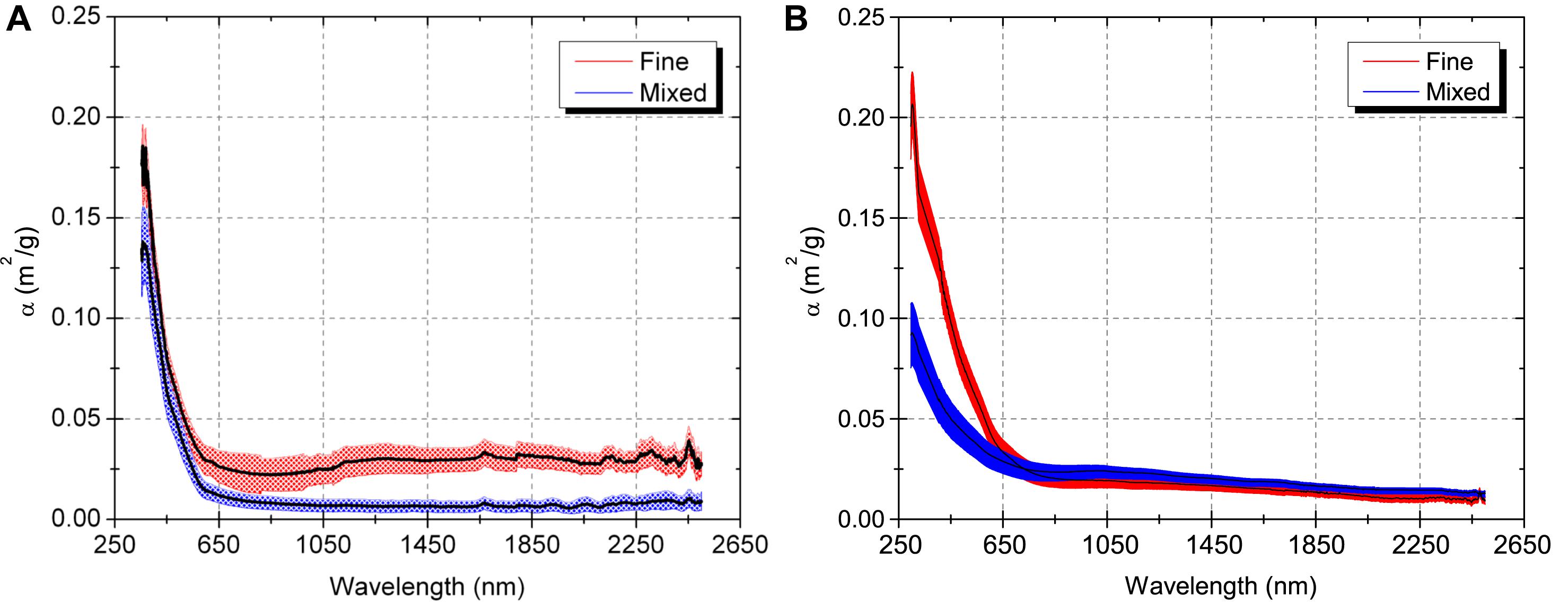
Figure 9. Spectral mass absorption efficiency (m2/g) for Saharan dust (A) and volcanic ash (B), measured as a continuous spectrum from 300 to 2350 nm. The sampled particles were size separated into a fine mode (<1 μm: red) and all sizes (blue). Panels taken from Rocha-Lima et al. (2014, Figure 8) and Rocha-Lima et al. (2018, Figure 7).
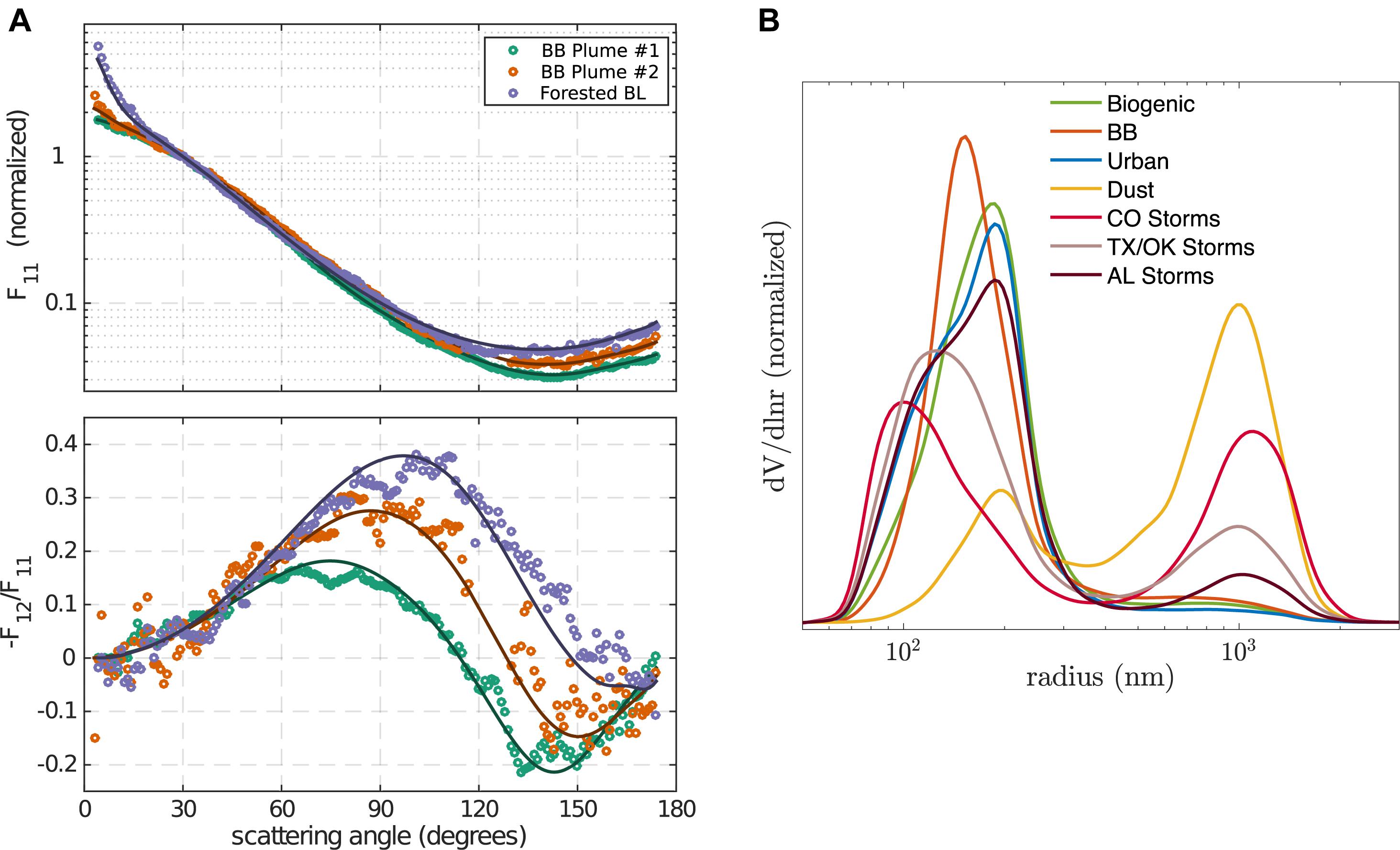
Figure 10. (A) Measured phase function (F11) in upper panel and degree of linear polarization (–F12/F11) in lower panel for three different samples encountered during the SEAC4RS campaign in North America in 2013. The samples include two different biomass burning plumes (BB plume) and a pass through a forest boundary layer heavy in biogenic aerosol (Forested BL). Shown are direct measurements from the UMBC PI-Neph, taken from Figure 5 in Espinosa et al. (2017). (B) Retrieved particle volume size distributions using the GRASP (Dubovik et al., 2014) retrieval software with PI-Neph inputs similar to those shown in the top panel. Different aerosol types after Espinosa et al. (2018) are shown. Data were collected during the DC3 (2012) and SEAC4RS (2013) field campaigns.
Advancements have also been made in aerosol height retrievals from OCI-like passive remote sensing data [e.g., Duforêt et al. (2007) and Dubuisson et al. (2009) from POLDER and MERIS (Medium Resolution Imaging Spectrometer) data]. Sensitivity studies on the information content of aerosol height over oceans in OCI’s hyperspectral measurements of Oxygen A- and B-band radiance are reported by Davis and Kalashnikova (2019), Frouin et al. (2019), and Remer et al. (2019). In addition, Xu X. et al. (2017) studied aerosol height retrievals over vegetated land from actual Oxygen B-band radiance measured by the EPIC (Earth Polychromatic Imaging Camera) instrument onboard the DSCOVR (Deep Space Climate Observatory) platform. One drawback of aerosol height retrievals from Oxygen A- and B-band radiance is that the aerosol optical thickness has to be sufficiently large (i.e., ≥0.3) at 550 nm when over relatively bright surfaces. A solution is to use multi-angle polarization measurements in the deep-blue, exploiting the decrease caused by aerosol scattering in the polarization originating from pure molecular scattering. These measurements are less sensitive to the surface (see e.g., Chowdhary et al., 2012), and allow aerosol height to be retrieved at lower aerosol optical depths as demonstrated by Wu et al. (2016) (see also Chowdhary et al., 2005). More information on aerosol height retrievals from these and other passive remote sensing data (e.g., from multi-angle radiance-only data) is provided in Xu et al. (2018).
Retrievals of absorbing gas column concentrations are important for the atmospheric science discipline. The ocean discipline benefits equally, if not more, from such retrievals. That is because accounting for absorbing gases in the atmosphere is an important part of the atmospheric correction process in the retrieval of the ocean remote sensing reflectance (Rrs – see definition in Table 2) from satellite observations. That process requires a better understanding of modeling non-gray gas absorption in vertically inhomogenous atmosphere in RT simulations. In NASA’s heritage ocean color retrievals, a simple gas correction of the TOA measurements, based on Beer’s–Lambert law treatment, is performed using ancillary or climatology gas column concentration from NOAA’s National Center of Environmental Predication (NCEP) (Derber et al., 1991; Gordon and Wang, 1994b; Kanamitsu et al., 2002; Ahmad et al., 2007; Dee et al., 2011). Traditional ocean color bands commonly are situated in atmospheric transparent windows to avoid the strong absorption features by O2 (Oxygen) and H2O (water vapor), which can not be treated with the simple Beer–Lambert RT equation. Nevertheless, the spectral bands of NASA’s heritage multi-spectral ocean color sensors, such as SeaWiFS (Sea Viewing Wide Field-of-View Sensor), MODIS, and VIIRS (Visible Infrared Imaging Radiometer), are still impacted by the absorption of some atmospheric gases, mainly O3 (Ozone) and NO2 (Nitrogen Dioxide), within the broad UV-VIS spectrum. For hyperspectral sensors, such gaseous absorption in the UV-VIS spectrum can be erroneously attributed to plankton spectral signature, degrading the plankton type detection capabilities, which are central to the PACE mission. In addition, the hyperspectral detection capabilities of the OCI instrument on-board the PACE mission will require thorough corrections for absorption by O2 and H2O, most importantly in the plankton fluorescence spectral range (∼685 nm). The O3 correction is possible with the OCI UV capability; however, NO2 correction is more challenging due to the insufficient spectral resolution in the UV. Since NO2 concentration can be significantly higher in coastal industrial regions, it can have a significant impact on the ocean reflectance retrievals in the blue spectral range (Tzortziou et al., 2018). Future research is necessary to address these concerns. The retrieval of, and subsequent correction for absorption by, Column Water Vapor (CWV) is a challenging task due to (i) the complexity of the CWV profile; (ii) the spectrally variable nature of CWV absorption features; and (iii) the spatial heterogeneity of CWV concentration. Similarly, the Oxygen A- and B-bands (at ∼760 nm and ∼687 nm, respectively) can also be challenging to utilize for ocean color retrievals due to the presence of scattering aerosols near the boundary layer of the atmosphere. Thus, a Beer’s–Lambert compensation of the water vapor and Oxygen bands, without consideration of the absorption-scattering coupling effects, the overlapping absorption of different gas species, and the inhomogeneous path, could lead to significant errors (Bouffiès et al., 1997; Dubuisson et al., 2004; Ibrahim et al., 2018).
The first challenge toward addressing the impact of absorption by H2O and O2 on OCI’s hyperspectral data is to quantify this impact. This, in turn, requires the use of RT methods that can properly handle all absorbing gases within OCI’s spectral coverage. That is, accurate RT simulations need to be performed at finer spectral resolutions than for heritage ocean color sensors to properly account for the narrow spectral features of H2O and O2. Brute force Line-by-Line (LBL) RT simulations are the most accurate (Gao et al., 2000, 2009), however, they are also very computational intensive. Several methods have been developed in the past to improve the efficiency of the LBL RT method, such as the band model method, the k-distribution method, the correlated-k distribution method, and the double-k method (Goody and Yung, 1989; Lacis and Oinas, 1991; Fu and Liou, 1992; Duan et al., 2005). The band model is the most efficient method since it analytically computes the transmittance of a homogenous path in the atmosphere for a wide range of absorber amounts. However, this method lacks sufficient accuracy for non-gray gaseous absorption, for vertically inhomogeneous atmospheres, and in the presence of scattering (Goody, 1952; Malkmus, 1967; Lacis and Oinas, 1991). The k-distribution method provides a highly accurate representation of the transmittance by grouping the gas LBL absorption features by strength within an arbitrary band, thus producing a smooth function that can be fitted with analytical expressions or represented by a relatively small number of bins. The k-distribution method is an exact alternative to the LBL method and the user can define the accuracy by defining the number of bins depending on the application with remarkable computational efficiency. To further increase the computational efficiency and accuracy in inhomogeneous atmosphere, the correlated-k method derives an analytical relationship between the k-distribution coefficients of multiple layers of the atmosphere at different pressure levels. Both the k-distribution and correlated-k provide accurate transmittance calculations for inhomogeneous atmosphere, overlapping gases, and in the presence of scattering in the atmosphere. However, the correlated-k method suffers in overlapping absorption between H2O and CO2 (Carbon Oxide) and in the Oxygen A-band (overlapping H2O and O2), where there is a poor vertical correlation (Lacis and Oinas, 1991). Note that Oxygen A- and B-bands are specifically important for PACE aerosol layer height retrievals and for the chlorophyll fluorescence detection, respectively (Dubuisson et al., 2001; Zhai et al., 2018). For example, Dubuisson et al. (2001) have utilized the Oxygen A-band to retrieve the aerosol layer height showing a significant underestimation of the scale height over dark ocean surfaces. Thus, Dubuisson et al. (2001) suggested a correction factor based on extensive RT simulations for varying aerosol optical depth and geometries, reducing the uncertainty by an order of magnitude. The importance of a correction factor due to the coupling effects was first highlighted by Frouin et al. (1990) to improve the CWV estimates over the dark ocean in the presence of scattering aerosols. Dubuisson et al. (2004) later formulated this method such that a correction factor as a function of geometry, aerosol optical depth and scale height is derived based on RT simulations to reduce CWV retrieval and correction uncertainties. A more recent method fits the hyperspectral measurements with analytical expressions involving both the total absorption optical depth and the absorption optical depth from TOA to the main scattering layer, which couples the absorption process with the scattering process in the atmosphere (Duan et al., 2005). A careful assessment of these methods in terms of numerical uncertainties and efficiencies are needed to determine an optimal method that can both satisfy the computational efficiency and accuracy conditions. In summary, the coupling effect of absorption and scattering in strongly absorbing spectral regions is problematic for ocean color remote sensing directly through imperfect correction of gas features that could be erroneously attributed to the ocean constituents or indirectly by impacting the assessment of the aerosol radiance necessary for the atmospheric correction (i.e., scale height, or out-of-band effects) (for example Dubuisson et al., 2001; Gordon, 1995). One suggestion to minimize these effects is to use a correction method as suggested by Dubuisson et al. (2001, 2004) for a large set of environmental conditions. Another possibility is to generate atmospheric correction algorithms (i.e., look-up tables, or LUTs) or gas retrieval algorithms with RT codes that inherently takes in consideration the strong gases absorption coupling with scattering; however, that could dramatically increase the dimension and complexity of the algorithm LUTs. A trade-off study would be necessary for such assessment in order to provide an optimal utilization to operationally capable algorithm for the PACE mission.
The second challenge toward addressing the impact of H2O and O2 absorption on OCI’s hyperspectral data is to retrieve and compensate for the CWV transmittance. In the EOS era, NIR data have been utilized as an alternative to thermal IR data to retrieve CWV over land and ocean (Chesters et al., 1983; Susskind et al., 1984). The feasibility to retrieve CWV amount using 940-nm water vapor band was first demonstrated by Gao and Goetz (1990) and Gao et al. (1993) using data collected by AVIRIS (Airborne Visible/Infrared Imaging Spectrometer) onboard the ER-2 aircraft platform and independently by Frouin et al. (1990) using data collected by a dedicated, aircraft-mounted radiometer. The retrievals were based on the differential absorption technique, where the ratio of the TOA reflectance in a window channel to a water vapor channel (or more generally in two channels differentially affected by water vapor absorption) is correlated to the water vapor amount along the path. CWV retrievals using the 940-nm channel are also limited to bright surfaces, such as land, ice, and clouds – and, over oceans, to sun glint regions. Over dark surfaces, as indicated above, the coupling between aerosol scattering and water vapor absorption, modulated by water vapor content, can be exploited to yield sufficiently accurate retrievals (Dubuisson et al., 2004). The differential absorption technique has been extended for application to MODIS data, where three water vapor channels with different sensitivities to moisture (i.e., 905, 930, and 940 nm) are utilized to retrieve the CWV at different amounts. The method by Gao and Goetz (1990) utilizes two window channels and one water vapor channel to remove the spectral dependency of the surface. This is achieved in the Frouin et al. (1990) method by utilizing two channels, one narrow, the other wide, centered on the same wavelength at the maximum of water vapor absorption. The three-band ratio technique applied to MODIS data uses a LUT search of pre-computed three band ratios of the water vapor transmittance using either LBL, MODTRAN (Moderate Resolution Atmospheric Transmission), or LOWTRAN (Low Resolution Atmospheric Transmission) calculations. The OCI instrument will have one wide 940 nm band with a 50 nm FWHM (Full Width at Half Maximum) as opposed to MODIS three water vapor channels. This limitation will allow CWV retrievals albeit with a less dynamic range. However, the MODIS approach hints that such retrievals may be improved using other additional water vapor bands that lie within the OCI spectral range such as 720 nm and 820 nm spectral regions.
Additionally, OCI will have spectral measurements capability in the UV with high radiometric quality that will allow for ozone retrievals using the simple differential absorption algorithm used for OMI data, but instead at high spatial resolution (Veefkind et al., 2006 and references therein). However, the UV spectral range requires rigorous multiple scattering calculations, since the scattering and absorption of air molecules is significantly enhanced at shorter wavelengths. The ozone vertical profile is required as a priori in order to estimate the ozone concentration. A RT benchmark analysis is required to improve the algorithmic uncertainties for ozone retrievals and corrections.
At the NASA Ocean Biology Processing Group (OBPG), FWD RT studies were conducted to test an operationally capable hyperspectral atmospheric correction (AC) method that accounts for gas absorption. A fully operational AC has been implemented and validated using proxy data sets from the HICO (Hyperspectral Imager for Coastal Ocean) and the AVIRIS instruments that resemble anticipated data from the OCI instrument (Ibrahim et al., 2018). This development was based on extending the multi-spectral AC algorithm to a hyperspectral one (Ahmad et al., 2010; Ibrahim et al., 2018). The main additional feature is the correction of water vapor, while other gases corrections are based on the ocean color heritage approach (Gordon and Wang, 1994b). The ATREM (ATmospheric REMoval) code was merged into the operational Level 1 to Level 2 (L2GEN) processing code, in order to primarily handle water vapor correction and CWV retrieval, for each pixel observation (Gao et al., 1993).
A k-distribution method was implemented in the current operational AC procedure to increase the computational efficiency of the LBL water vapor transmittance calculations without compromising the accuracy (Lacis and Oinas, 1991; Kato et al., 1999). A pre-computed table of k-distribution coefficients was stored for every band and layer of the atmosphere, and the corresponding AC method was tested and validated by applying the algorithm to HICO proxy data retrievals and comparing against in situ observations of the ocean remote sensing reflectance Rrs obtained from SeaBASS (SeaWiFS Bio-optical Archive and Storage System) and AERONET-OC(Ocean Color). Note that while the k-distribution ignores coupling effects between gaseous absorption and scattering in narrow spectral features such as the O2 bands, its implementation proved to be simple and accurate for band-averaged transmittances. As an illustration, Figure 11 below shows the retrieval of the hyperspectral Rrs from HICO observations at the Chesapeake Bay region on the east coast of the United States, as compared to MODIS Aqua multi-spectral retrievals. The Rrs retrievals are shown for three different locations in the Bay water. Note that the agreement seen for the MODIS and HICO retrievals of Rrs is desirable and expected for a wide dynamic range, since both sensors are vicariously calibrated at the same site and processed with the same atmospheric correction algorithm. However, the wealth of the hyperspectral Rrs information from HICO or OCI is expected to significantly improve ocean color products provided that AC includes a proper handling of gases absorption for all wavelengths.
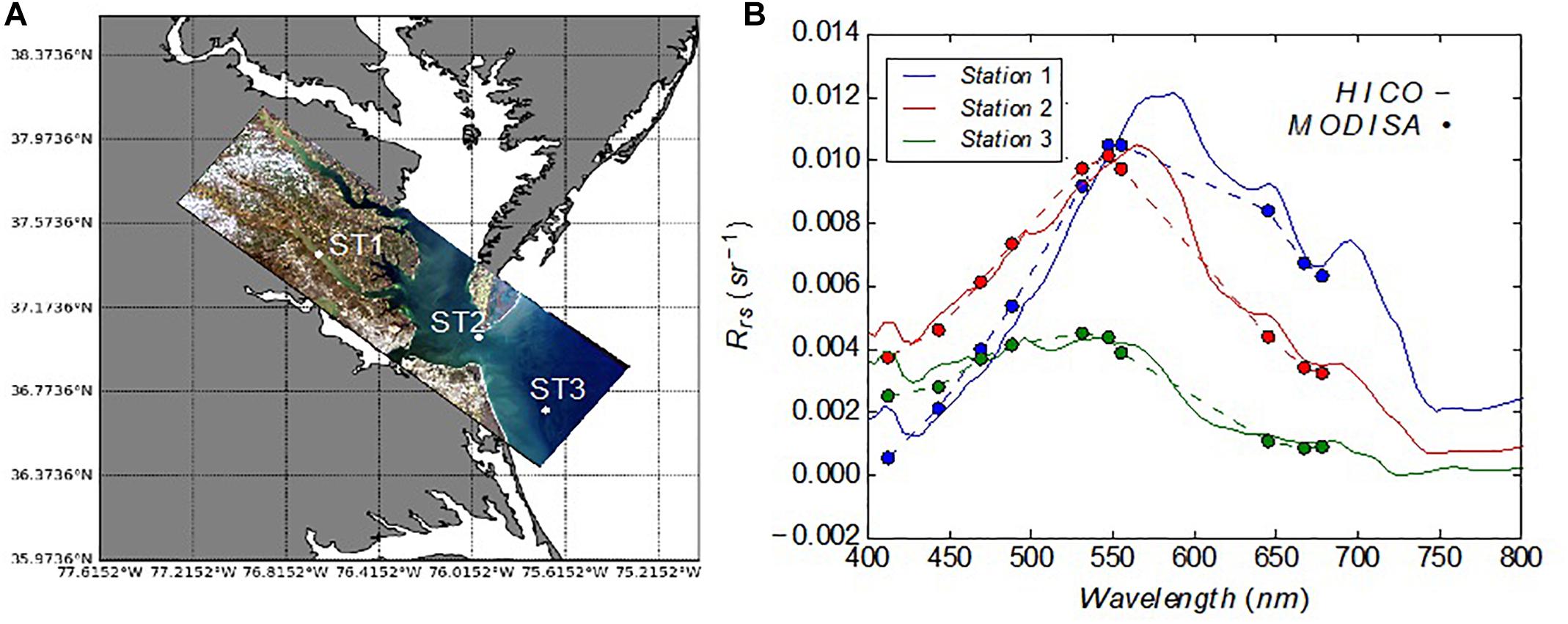
Figure 11. (A) HICO true color image at the Chesapeake Bay waters. (B) the retrieved Rrs at three different locations from HICO and MODIS Aqua after atmospheric correction and water vapor correction using the k-distribution method for gaseous absorption. This figure has been adapted from Ibrahim et al. (2018).
The OCI instrument will continue the heritage CWV retrieval using the 940-nm band. However, compared to MODIS’ three bands near the 940 nm regions (905 nm, 935 nm, and 940 nm) that each have different sensitivities to water vapor amount, OCI’s 940-nm band has a wider spectral resolution and will be less sensitive to large water vapor amounts over dark surfaces due to saturation of absorbing amounts and small SNR. Water vapor correction using OCI’s 940-nm band over the dark ocean is therefore not optimal. However, Ibrahim et al. (2018) showed a better water vapor correction can be obtained by utilizing the less saturated 720 nm and 820 nm bands (or a combination of both) on OCI, especially for large water vapor amounts. The analysis shows less systematic bias in CWV retrievals over the ocean than using only the 940-nm band. Based on extensive RT simulations, the retrieval error using a combination of 940 and 820 nm, 720 and 820 nm, and 720 nm only is 19, 8.5, and 9%, respectively. CWV retrievals uncertainty using the 720 and 820 nm bands corroborates with the ones retrieved by microwave radiometry over dark oceans (Gao and Kaufman, 2003). A combination of the three strongly absorbing water vapor bands (720, 820, and 940 nm) within the OCI spectral coverage will therefore allow retrievals of CWV with large dynamic range, over land and ocean. It is important to note that retrieving the CWV using NIR bands does not necessarily mean a proper compensation of the water vapor transmittance at some of the visible bands. This is primarily due to the dependence of the water vapor transmittance on the vertical profile of water vapor and temperature/pressure, which is currently assumed to be the US standard 1976 (Anderson et al., 1986). Current efforts within the PACE team are being taken to supplement the vertical profile information from ancillary sources such as NASA’s Goddard Earth Observing System Model, Version 5 (GEOS-5) provided by the Global Modeling and Assimilation Office (GMAO) which provides 3-h instantaneous vertically resolved specific humidity that can scale the observed data (Gelaro et al., 2017).
Synthetic data generated by RT solvers will be used to test future PACE atmospheric correction algorithms. It is important for such data to properly account for gas absorption in cases of (i) non-narrow (e.g., overlapping) absorption bands, and (ii) particle scattering interaction. These cases are not well handled by the k-distribution. The double-k method has been applied to a RT model that accounts for all major light matter interaction mechanisms, including gas absorption, scattering and absorption by particulates in atmosphere and ocean, atmosphere and ocean coupling, and inelastic scattering mechanisms in ocean waters. The base line of the model is the RT model developed by Zhai et al. (2010, 2015, 2017a). Gas absorption from water vapor, oxygen, ozone, nitrogen dioxide, methane, and carbon dioxide are included. First, hyperspectral lookup tables of gas absorption coefficients have been built using the atmospheric radiative transfer simulator (ARTS) (Buehler et al., 2011) based on the HITRAN (HIgh Resolution TRANsmission molecular database) 2012 database (Rothman et al., 2013) for water vapor, oxygen, carbon dioxide, and methane. Absorptions by ozone and nitrogen dioxide are included separately using measurements of Daumont et al. (1992) and Bogumil et al. (2003). For each measurement channel, we choose several representative gas absorption optical depths, and run the full RT that couples gas absorption and scattering. We then apply the double-k method (Duan et al., 2005) to fit the full hyperspectral line-by-line radiance using the radiance values at wavelengths with known absorption optical depth. The instrument radiance is found by integrating the fitted spectral radiance with the instrument line shape function. Generally a high accuracy of 0.1% can be achieved using the double-k method in comparison to the exact line-by-line RT simulations. In Ibrahim et al. (2018), we used this implementation to show that ignoring the coupling between water vapor absorption and particulate scattering in simulating spaceborne NIR radiance between 600 and 800 nm leads to an error between 0 and 10% for one particular case with an aerosol optical depth of 0.2 at 550 nm. The error becomes larger for more absorptive bands. This highly accurate model is therefore suitable to generate synthetic PACE science data for studies on CWV retrievals in the NIR and/or correction for gaseous absorption in the VIS.
The current literature contains a multitude of benchmark results to validate vector RT computations in isolated slabs of atmosphere. Tabulated results can be found for homogeneous atmospheres containing molecules only (Coulson et al., 1960; Stammes et al., 1989; Mishchenko, 1990; Natraj et al., 2009; Natraj and Hovenier, 2012), for (in-) homogeneous atmospheres containing (molecules and) aerosols (de Haan et al., 1987; Wauben and Hovenier, 1992; Siewert, 2000), and for homogeneous atmospheres consisting of cloud droplets (Kokhanovsky et al., 2010). However, there exist no tables for the polarized radiance computed for AOS models. Although comparisons for polarized RT computations using different RT codes have been reported (e.g., Zhai et al., 2010; Hollstein and Fischer, 2012; Chami et al., 2015), the results are drawn as a function of viewing angle which limits the accuracy that can be extracted to validate other RT codes. Current and future remote sensing polarimeters can measure the DoLP to an accuracy of 0.1–0.5%, which requires that the RT codes used to analyze these measurements must be validated to at least the same accuracy. Even quantitative RT results for just the intensity of light computed for AOS models are rare to find (Mobley et al., 1993; Bulgarelli and Doyle, 2004).
To provide accurate tabulated results for the total and linear polarized upwelling radiance just above the ocean surface (SRF) and at the top of the atmosphere (TOA), RT computations were performed (Chowdhary et al., “Benchmark results for scalar and vector radiative transfer computations of light in atmosphere-ocean systems”, unpublished) for different viewing geometries, wavelengths, and AOS models (see Figure 12). The viewing geometries for these tables scan the upwelling radiance in the solar principal plane (azimuth angle φ = 0° and 180°) and in an off-principal plane (azimuth angle φ = 60° and 240°) for viewing angle θ that ranges between 0° and 60° (measured with respect to the surface normal) in steps of 5°. Two sun angles (θ0 = 30° and 60°) are considered for each scan; hence, the viewing geometries include the backscattering direction, the sun glint region, and observations that graze neutral polarization points seen in actual airborne observations (Kawata and Yakazaki, 1998) and in simulations (Adams and Kattawar, 1997; Chowdhary et al., 2012). Four wavelengths (350, 450, 550, and 650 nm) are chosen for these tables to sample the UV-VIS-NIR part of the spectrum that is monitored by the PACE mission. Furthermore, four hypothetical AOS models are used for our computations. They increase gradually in complexity from (i) a purely molecular atmosphere above a wind-ruffled ocean surface (taken from Cox and Munk, 1954) with no ocean body (AOS-I model); to (ii) a pure ocean water body below a wind-ruffled ocean surface with no atmosphere (AOS-II model); onward to (iii) a fully coupled simple atmosphere-ocean system body (AOS-III model) containing a molecular atmosphere, wind-ruffled ocean surface and pure ocean water; and finally to (iv) a coupled complex atmosphere-ocean system (AOS-IV model), that includes scattering by molecules, wind-ruffled ocean surface, pure ocean water, and sharp forward-scattering marine particulates [i.e., the D-P mixture taken from Chowdhary et al. (2012), with [Chla] = 0.03 mg/m3 at 350 and 450 nm and [Chla] = 3.00 mg/m3 at 550 and 650 nm]. Some results presented for the AOS-I model can be compared with those reported for an isolated molecular atmosphere by Natraj et al. (2009) if the optical thickness is set to 0.5 (this model is denoted by AOS-I∗), whereas the purpose of the advanced AOS-IV model is to produce realistic values for SRF and TOA observations. All computations were performed thrice using RT codes that are based on different RT methods, i.e., the Doubling-Adding RT code eGAP described in Chowdhary et al. (2006), the Successive-Order-of-Scattering RT code SOS-CAOS described in Zhai et al. (2009, 2010), and the hybrid Markov-Chain-Adding-Doubling RT code MarCH-AD described in Xu et al. (2016). For these computations, the number of underwater light quadrature points used for AOS-I and AOS-III models was set at 80 to adequately capture refraction of light by the ocean surface, while in AOS-IV model it was set at 300 to capture the sharp unnormalized diffraction peaks (corresponding asymmetry parameters ≥ 0.95) for scattering by D-P particulates. A fourth code, i.e., the Monte Carlo RT code SMART-G described in Ramon et al. (2019), was also used for OAS-I model computations in which the rough ocean surface was treated as a BRDF surface. The number of photons used for the latter computations was set at 3 × 10¹¹. In total, Chowdhary et al. (“Benchmark results for scalar and vector radiative transfer computations of light in atmosphere-ocean systems”, unpublished) provide more than 25,000 tabulated RT results in units of reflectance. The stated reflectance accuracies for these tables, based on the maximum absolute difference in reflectance values obtained from the 3+ RT code computations, is better than 10−5 for AOS-I and AOS-IV models, and better than 10−6 for AOS-II and AOS-III models. The corresponding DoLP values vary by less than 0.2% for a handful of tabulated reflectance values, and by less than 0.1% for all other scattering geometries, atmosphere-ocean systems, wavelengths, and altitudes considered in this work. This satisfies the forward RT accuracy requirement to match the measurement accuracy for all PACE satellite instruments (cf. “1.1 The PACE Mission” section).
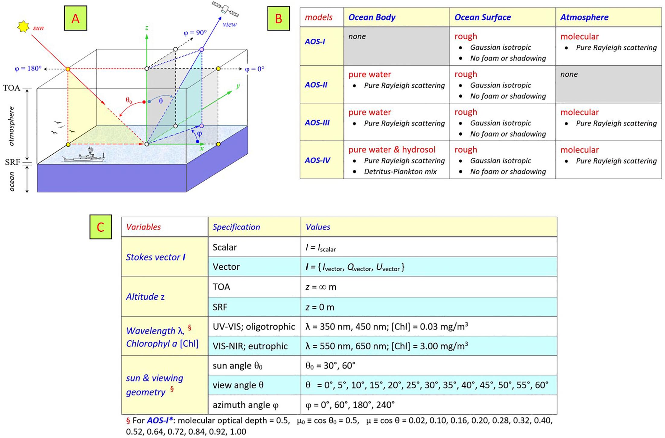
Figure 12. (A) Schematic illustration of Atmosphere-Ocean System (AOS) model and scattering geometries used for RT benchmark computations. (B) Specification of AOS models shown in sub-panel (A). (C) Specification of variables used for each AOS model computation.
All the RT and retrieval studies mentioned thus far in this chapter approximate AOS models to be plane-parallel and horizontally homogeneous, i.e., they ignore the Earth’s curvature and horizontal variations in the atmosphere (e.g., small-scale aerosol plumes and broken clouds) and ocean (e.g., turbid eddies, isolated sea ice patches, and land-water boundaries). These approximations simplify, and therefore speed up, the numerical implementation of RT computations and retrieval algorithms. Cases for which these simplifications are not valid are either avoided or require addition numerical corrections.
Monte Carlo RT methods have a natural ability to handle 3-dimensional scattering media, and are therefore are particularly well suited to study light propagation in spherical AOS models. However, the large computational effort required for these methods can become burdensome, especially if the need for higher accuracy and/or smaller spatial resolution increases. One approach to reduce this burden is to trace the light backward from the detector to the source. This so-called Backward Monte Carlo method has been used in a number of studies (Collins et al., 1972; Adams and Kattawar, 1978; Ding and Gordon, 1994; Oikarinen et al., 1999) to examine scattering of light in spherical atmospheres. Such studies and other ones based on different RT methods (e.g., Herman et al., 1995; Rozanov et al., 2001; Doicu and Trautmann, 2009) show that the radiance emerging from spherical atmospheres can deviate noticeably from the one for plane-parallel approximated atmospheres even for small viewing angles θ (measured with respect to the surface normal), that deviations increase with solar zenith angle θ0 for θ0 ≥ 60°, and that (depending on the aerosol type and load) these deviations cannot be ignored anymore if the solar zenith angle θ0 becomes larger than 70°.
A commonly used correction for deviations occurring at large solar zenith angles is to only attenuate the direct solar beam by a spherical atmosphere while still using the plane-parallel approximation to compute the contribution of light scattered in the atmosphere (Dahlback and Stamnes, 1991). To improve the accuracy, single scattering may further be calculated in full spherical geometry (Spurr, 2002). Such pseudo-spherical approaches may still fail at solar zenith angles θ0 ≥ 85° (Caudill et al., 1997). More importantly, they do not address deviations from RT results obtained for plane-parallel atmospheres that can occur at small solar zenith angles. Another approach, described by Ding and Gordon (1994), is to only replace the radiance scattered by molecules in a plane-parallel atmosphere by the corresponding radiance scattered in a spherical atmosphere. This approach works well for solar zenith angles θ0 > 70°, but again does not affect much the RT results obtained for small solar zenith angles. Finally, we remark that while some of the above-mentioned studies (Rozanov et al., 2001; Doicu and Trautmann, 2009) consider the presence of a Lambertian ground surface (albeit ignoring the polarization of light in RT computations), none of them consider an ocean surface below a spherical atmosphere. The bidirectional and polarizing properties of an ocean surface strongly affects the radiance and polarization of light emerging from the top of the atmosphere, and may therefore change the impact that a spherical atmosphere has on RT computations for AOS models. There are RT methods available to study such phenomena (e.g., Xu et al., 2013), but they have not yet been applied to OCI studies for Earth.
AOS scenes exhibiting horizontal variations pose yet another problem in RT simulations. For atmospheric correction of ocean-color imagery, it is generally assumed that the target is horizontally homogeneous, or equivalently that the target is infinitely large. This “large target” formalism is generally appropriate in the open ocean, sufficiently far from clouds and land, since the intrinsic atmospheric reflectance (i.e., the signal that has not interacted with the water body) is the main perturbing signal. In the vicinity of land, near sea ice or clouds, and even where horizontal heterogeneity is large (case of upwelling areas), the impact of photons reflected by the environment of the target and scattered into the field of view may not be negligible and may yield erroneous water reflectance retrievals and derived biogeochemical variables (e.g., Tanré et al., 1981; Santer and Schmechtig, 2000). The problem is not only the adjacency effect at the wavelength of interest, i.e., UV to visible, but also (in some cases more importantly) the propagation to shorter wavelengths of errors in the determination of aerosol scattering in the red and NIR. At these wavelengths the environment reflectance is seen in the atmospheric correction scheme as part of the aerosol reflectance. The atmospheric variables controlling the adjacency effect are the aerosol amount (optical thickness) and altitude, and to a lesser extent the aerosol model (see Frouin et al., 2019).
The SMART-G radiation transfer code (Ramon et al., 2019) was used to examine the effects of Earth’s sphericity on the radiance emerging from the atmosphere. This code is based on the Monte Carlo technique, works in either plane-parallel or in spherical-shell geometry, and accounts for polarization. A local estimate variance reduction technique (Marchuk et al., 1980; Rakimgulov and Ukhinov, 1994) is implemented for the radiance calculations. In spherical mode, the change in photon path due to index of refraction variations with altitude is neglected, which reduces accuracy at grazing angles and in twilight conditions. Inelastic processes (e.g., Raman scattering) are not taken into account. SMART-G is written in CUDA (Compute Unified Device Architecture) and runs on GPUs (Graphic Processing Units). For typical simulations, an acceleration factor of several hundred is obtained using the GPU-based code compared with CPU (Central Processing Unit) computing. This makes SMART-G competitive, in terms of computational burden, with codes based on other RT methods (e.g., discrete ordinate, doubling-adding, successive orders of scattering), while allowing maximum flexibility.
SMART-G was run with 1 billion photons in backward mode (to avoid common problems associated with forward calculations, see above) for benchmark model AOS-I∗, i.e., a pure Rayleigh atmosphere with optical thickness of 0.5 (see Section “3.4.3 RT Validations”). The top of the atmosphere was at 120 km and molecule concentration decreased exponentially with increasing altitude (scale height is 8 km). Figures 13, 14 display some of the results, i.e., for Stokes parameters I, Q, and U (normalized into reflectance units) and the DoLP as a function of viewing angle θ (measured with respect to the surface normal) for the 0°–180° and 60°–120° azimuth planes. Cosine of the sun zenith angle θ0 is set to 0.6. Absolute and relative differences with respect to benchmark results (Chowdhary et al., “Benchmark results for scalar and vector radiative transfer computations of light in atmosphere-ocean systems”, unpublished) are also displayed. In the plane-parallel approximation, the reflectance values for I, Q, and U generated by the two codes agree to better than 0.00002 (absolute), and the corresponding DoLP values to better than 0.01 (absolute). For Stokes parameter I, the relative difference is less than 0.01%. The typical effect of sphericity is to lower intensity I by 0.3–0.5% for viewing angles θ < 50° and up to 2% at larger viewing angles, and to change the polarization ratio DoLP by 0.3–0.4%. This is due to a reduced illuminated volume in spherical-shell approximation (smaller optical path, all the more as the view angle is large). Note that this view angle (θ) effect, which in first approximation varies as the ratio of the spherical-shell and plane-parallel optical paths, i.e., cos(θ)[(cos2(θ) + 2η + η2)1/2 – cos(θ)]/η, where η is equal to h/RE with h the height of the atmosphere and RE the Earth radius, would appear negligible at small view angles if h is not large enough. For example h = 20 km, used in the simulations performed by Ding and Gordon (1994), is too small (at θ = 30°, the ratio would be 0.9995 for h = 20 km instead of 0.9969 for h = 120 km). The other important effect of sphericity (well known but not illustrated here) is an intensity increase at grazing solar zenith angles (θ0 > 80°) due to the smaller attenuation of the direct solar beam, again because of the smaller optical path. In view of the accuracy requirement for water reflectance ρw, i.e., ±5% or ± 0.002 in the blue for clear waters (“1.1 The PACE Mission” section), and since at blue wavelengths typically 90% of the signal observed from space originates from the atmosphere, mostly due to molecular scattering, the above results indicate that neglecting Earth’s sphericity in generating Rayleigh look-up tables may introduce errors comparable to (i.e., up to 5% for θ < 50°) or even larger than (i.e., up to 20% for θ0 > 80°) the PACE accuracy requirement for ρw. Earth’s sphericity, therefore, needs to be taken into account in the molecular scattering calculations, even at small viewing angle θ, for accurate ocean-color remote sensing from space, in addition to molecular number density, index of refraction, and anisotropy of molecules.
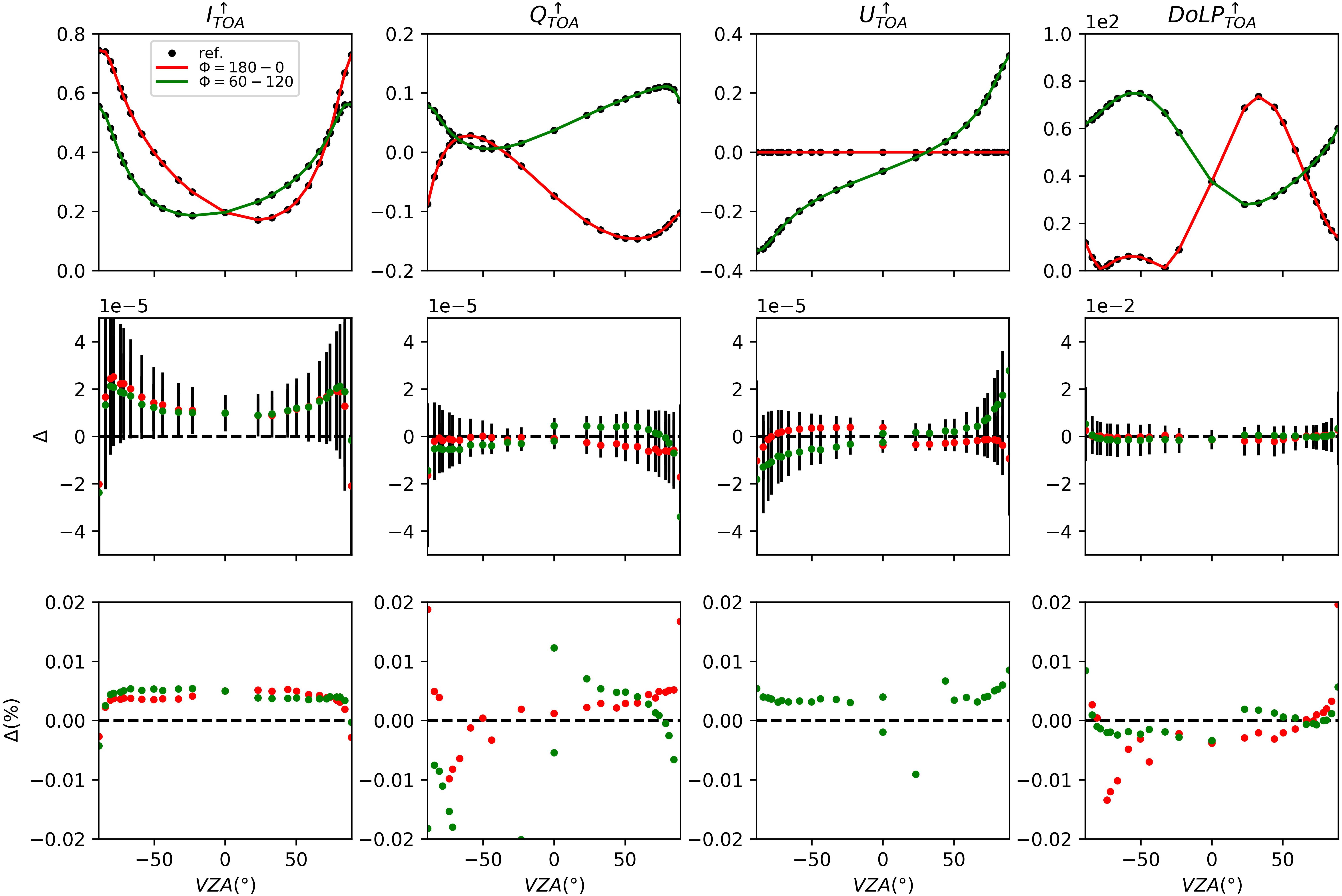
Figure 13. Comparison of benchmark results for AOS-I∗ model (Chowdhary et al., “Benchmark results for scalar and vector radiative transfer computations of light in atmosphere-ocean systems”, unpublished) computed with the NASA/GISS RT code and the Monte Carlo code (plane-parallel atmosphere) as a function of view angle θ (measured with respect to the surface normal) for relative azimuth angles of 0°, 60°, 120°, and 180° (red and green curves). Absolute differences are <0.00002 for the reflectance values of I, Q, and U, and relative differences are generally <0.02% for DoLP.
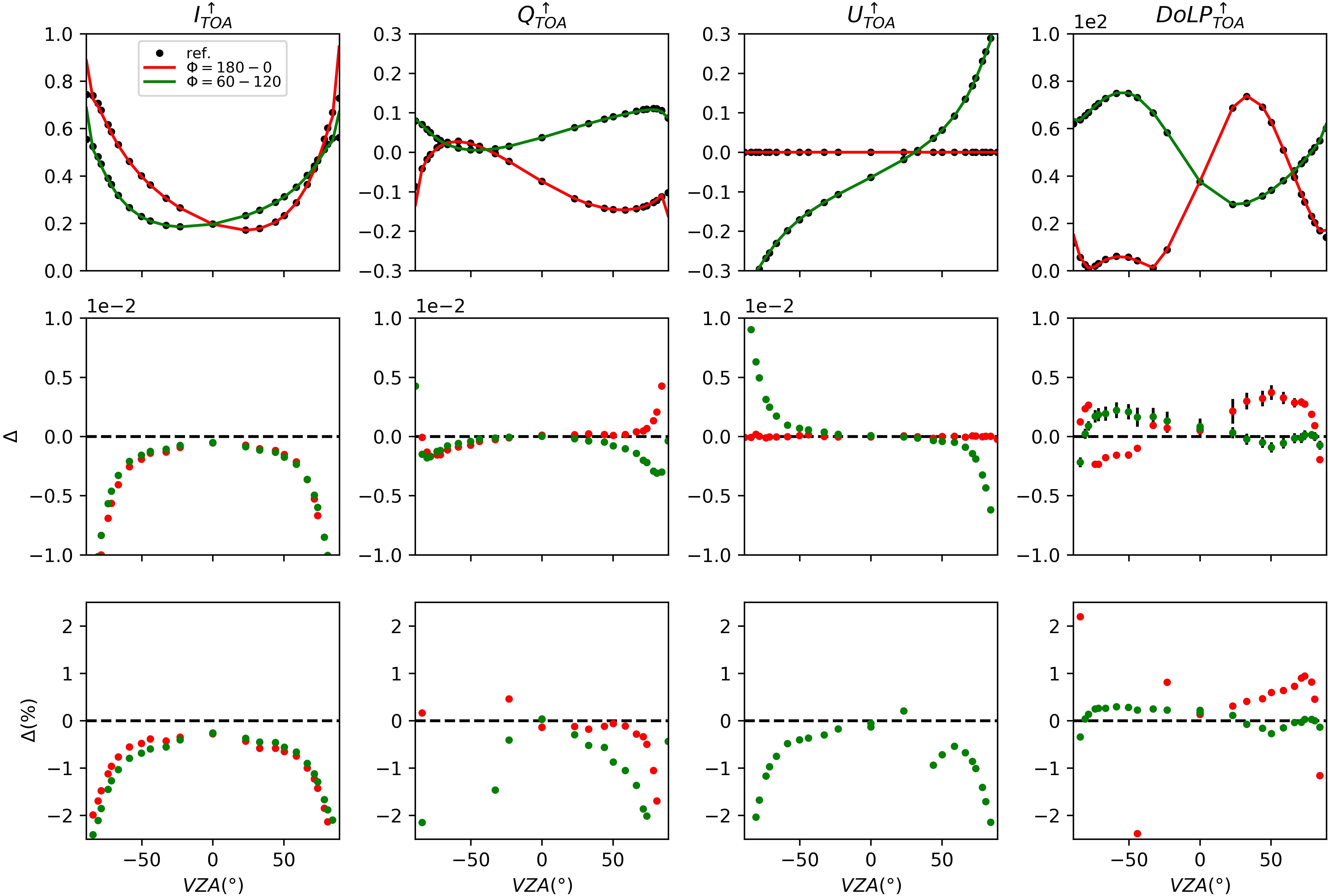
Figure 14. Same as Figure 13, but spherical-shell atmosphere for Monte Carlo code. The effect of sphericity is to lower intensity I by 0.3–0.5% for viewing angles θ < 50° and up to 2% at larger viewing angles, and to change polarization ratio DoLP by 0.3–0.4%.
Adjacency effects, due in particular to horizontal heterogeneity of surface reflectance, can be simulated with a Monte Carlo code such as SMART-G. The typical procedure consists in applying, in backward mode, a given 2-dimensional surface reflectance function that depends on the photon’s horizontal coordinates. The photons are injected from the viewing direction toward the surface point of Cartesian coordinates (x, y) for which the adjacency effect is to be estimated (the target). This point is considered at the center of the x–y plane. Then using the local estimate method (or a cone sampling method), the Stokes parameters are computed for the solar geometry. Due to atmospheric scattering, some of the photons exiting the atmosphere in the solar direction experience one or multiple reflections at the surface outside the target, and may not interact with the target. The atmospheric spread function f(x, y), i.e., the fraction of radiance that leaves the surface at (x, y) and scatters within the field of view when targeting the point (0, 0), can also be computed (photons experiencing surface reflection can be counted), allowing calculation of the environment reflectance and, therefore, the adjacency effect.
Figure 15 displays SMART-G simulations in the plane-parallel approximation of the adjacency effect on the TOA reflectance at 412, 670, and 865 nm of a water target next to a rectilinear coastline separating land and ocean. [The adjacency effect, Δρ, is indicated as the difference between the actual reflectance (defined in Table 2) at TOA and the reflectance that would be measured if the surface were horizontally homogeneous.] The reflectance of the land surface, assumed Lambertian, is 0.05, 0.1, and 0.3, respectively (typical green vegetation), and phytoplankton chlorophyll concentration is 0.1 mg/m3 (Case I waters). Aerosol are of maritime type, with an optical thickness of 0.2 at 550 nm and an aerosol scale height of 2 km (exponential profile), and the ocean surface wind speed is 5 m/s. View zenith angle is 45° and relative azimuth angle is 90°. The azimuth angle of the Sun is along the coastline. At 2 km from the coast, i.e., right panels, Δρ is generally positive, especially in the NIR where vegetation reflectance is high compared to that of the water (negligible). For small Sun angles (<20°), Δρ is about 0.005, 0.002, and 0.001 at 865, 670, and 412 nm, which represents about 25, 5 and <1% of the actual reflectance. The effect decreases with increasing Sun angle θ0 with increasing view angle θ, due to increasing diffuse atmospheric transmittance. Using TOA observations in the red and NIR for atmospheric correction, the impact of Δρ on water reflectance retrieval at 412 nm is expected to be large, much larger than the Δρ at 412 nm caused by adjacency effect. Note that Δρ also depends on the sensor location (over the ocean or over land), an effect due to Fresnel reflection that may be masked for some angular configurations (Santer and Schmechtig, 2000). This masking effect would be more pronounced if the principal plane were perpendicular to the coast. Regarding polarization, the adjacency effect is opposite (more light, less polarization), i.e., the difference in DoLP (denoted by ΔDoLP) is generally negative, about 3% at 865 nm. For a given geometry, i.e., solar angle θ of 56° in the left panels, Δρ decreases in magnitude with increasing distance from the coast (same for ΔDoLP), but the effect is still felt at 10 km (4% at 865 nm), which is sufficient to yield unacceptable errors (i.e., > 0.002) on retrieved water reflectance at 412 nm (cf. “1.1 The PACE Mission” section). Only effects of distance and geometry for a typical aerosol are displayed in Figure 15, but aerosol parameters, especially vertical distribution (not easy to estimate from passive radiometry) also affect Δρ and ΔDoLP.
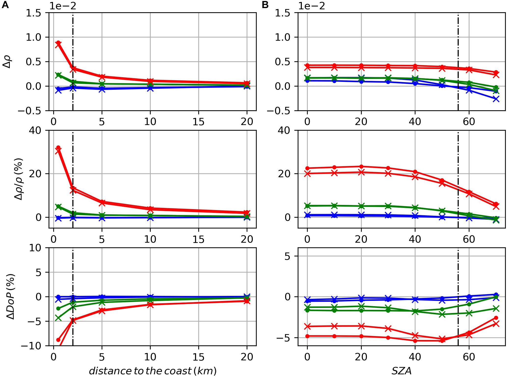
Figure 15. Monte Carlo simulations of adjacency effects on the TOA reflectance of a water target next to a rectilinear coastline. Wavelengths are 412, 670, and 865 nm (blue, green, and red curves). (A) Absolute and relative TOA reflectance and degree of linear polarization differences between cases of heterogeneous and homogenous surface as a function of distance to the coast. Solar and view angle are 56° and 45°, and relative azimuth angle is 90°. (B) Same as panel (A), but as a function of the Sun zenith angle (SZA, in degrees) for a distance to the coast of 2 km. Curves with solid circles correspond to the sensor located over ocean and curves with crosses to the sensor located over land.
Including hyperspectral UV-A radiance in observations by the OCI and SPEXone instruments offers new opportunities for atmospheric correction and ocean color product retrievals that were not possible with heritage ocean color missions. But studying these new opportunities by means of RT computations for UV-A radiance comes also with the need to more carefully consider (i) enhanced scattering in atmosphere and ocean of UV-A radiance; and (ii) changes in UV-A atmosphere and ocean scattering properties. In addition, one needs to consider variations in UV solar irradiance, which can happen on timescales of days (Lean, 1987) and which exceed those for the VIS-NIR spectrum by an order of magnitude (Lean and DeLand, 2012). Using prescribed solar irradiance spectra that do not incorporate such short-term temporal variations may lead to hyperspectral artifacts in retrieved water-leaving radiance that, in the UV-A toward the blue, easily exceed 0.002 in reflectance units. This was demonstrated by Thompson et al. (2015) in analyses of airborne hyperspectral data from the PRISM (Portable Remote Imaging Spectrometer) instrument. One of the requirements for PACE observations in the UV-A (toward the blue) is to retrieve water-leaving radiance within 10%. Determining the contribution of UV solar irradiance variations to the uncertainty in water leaving radiance, and its reduction through the use of TSIS (Total Solar Irradiance Sensor) observations if available, remains a subject for future studies. Here, we focus on subjects concerning RT of UV-A radiance in coupled atmosphere-ocean systems. In what follows, we will first summarize some of the main benefits of OCI/UV-A radiance for retrieving ocean and atmosphere properties before discussing concerns for simulating and analyzing TOA observations of UV-A radiance.
A major challenge in traditional atmospheric correction methods (i.e., methods that rely on NIR-SWIR radiance to constrain and remove aerosol scattering contributions in VIS space-borne radiance observations) is identifying the single scattering albedo (ωaer) and vertical distribution (Zaer) of aerosols (see Frouin et al., 2019). Changes in ωaer affect the amount of radiance absorbed in a single-scattering event before reaching the TOA. In the VIS, the impact of ωaer on TOA radiance is further enhanced by repeated aerosol-molecule light interactions. Because the molecular density decreases with height z, the amount of repeated aerosol-molecule light interactions becomes also dependent on the vertical location of aerosols. To properly extract ocean contributions from TOA radiance in the VIS therefore requires knowledge of both ωaer and Zaer. Section “3.3.1 Aerosols” discusses examples of using Oxygen A- and B-bands in the NIR, and of polarization in the deep blue, to obtain information on Zaer. That section touches also on using UV-A radiance to retrieve on Zaer. UV-A radiance becomes very sensitive – even more than VIS radiance – to variations in ωaer and Zaer because the molecular optical depth increases at a rate proportional to λ−4 (Bodhaine et al., 1999). This was confirmed by Levelt et al. (2006) and Torres et al. (2005, 2007) in analyses of UV observations by the TOMS and OMI instruments. In a follow-up study, Satheesh et al. (2009) demonstrated that one can retrieve both ωaer and Zaer from OMI/UV radiance if one uses MODIS/NIR-SWIR radiance to constrain τaer. Note that MODIS and OMI measurements do not occur simultaneous which can cause retrieval biases in the presence of clouds that evolve in the time lag between those measurements. This was demonstrated in a recent work by Gassó and Torres (2016). However, retrievals of ωaer and Zaer from OCI radiance measurements in the UV-A will not suffer from this limitation because OCI provides simultaneous radiance measurements in the NIR/SWIR to constrain τaer.
Historically, Chlorophyll a concentration [Chla] has been the most common property retrieved from heritage ocean color satellite data – and it continues to be one of the core ocean color products for the PACE mission (NASA, 2018a). Chlorophyll a affects the color of the ocean in the VIS by absorbing in the blue part of this spectrum – specifically, by its absorption peak at 443 nm. Most heritage [CZCS (Coastal Zone Color Scanning Experiment), SeaWiFS] and current [MERIS, MODIS, VIIRS] ocean color satellite instruments therefore measure radiance at, amongst others, a wavelength band centered at around 440 nm. The retrieval of [Chla] then proceeds (Blondeau-Patissier et al., 2014, and references therein) by using empirical relationships that fit either (i) so-called band ratios that consist of the ratio of the radiance at ∼443 nm and a radiance obtained in the green part of the VIS (Dierssen, 2010), or (ii) the IOPs retrieved from the radiance at ∼443 nm and at other wavelengths (the empirical relationships used in this approach are the bio-optical equations discussed in Section “Bio-Optical Models”). However, as is shown explicitly in Eqs 9 and 10, detrital matter and CDOM also absorb at 440 nm. Of these two ocean constituents, CDOM can absorb as much (if not more) as [Chla] at ∼443 nm, and its absorption decreases with increasing wavelength just like the absorption spectrum of [Chla] (Nelson and Siegel, 2013). This makes it particularly difficult to separate changes in [Chla] from variations in CDOM using the above-mentioned band ratio algorithms (see, e.g., Siegel et al., 2005). Bio-optical equations such as those discussed in Section “3.1.2 Bio-Optical Models” explicitly separate absorption by [Chla] (using pre-described Chla-specific phytoplankton absorption coefficients âph) from absorption by CDOM (which, in practice, is often combined with a relatively small contribution of absorption by detrital particulate matter). However, bio-optical equations are used for analyses of absolute water-leaving radiance measurements which are more susceptible to errors in atmospheric correction than the ratio of such radiance measurements. The aforementioned difficulties in constraining ωaer and Zaer from NIR-SWIR radiance will therefore impact bio-optical equations-based ocean product retrievals more than band ratio-based ocean product retrievals. In either retrieval method, UV-A radiance offers a better alternative to separate CDOM absorption than the radiance at 443 nm. That is because CDOM absorption continues to increase with decreasing wavelength (see, e.g., Eq. 8b), whereas Chlorophyll a absorption decreases in the UV-A. As a result, the relative contribution of CDOM absorption to total underwater light absorption (i.e., including absorption by Chlorophyll a, detrital matter, and water) increases from about 50% at 400 nm to >70% at 300 nm (Nelson and Siegel, 2013). Indeed, Morel et al. (2007a) conclude in their analyses of irradiance measurements obtained for two extreme open ocean regimes (i.e., South Pacific and Mediterranean waters) that the dominance of [Chla] in modeling bio-optical properties in the VIS is replaced by that of CDOM in the UV.
Light scattering contributions to TOA observations over oceans also exhibit regime changes when comparing VIS to UV-A radiance. Figure 16 illustrates these changes for an extreme case, i.e., for surface waters of the eastern South Pacific Gyre which have anomalously low [Chla] (Morel et al., 2007b; Claustre et al., 2008) and CDOM amounts (Morel et al., 2007a; Nelson and Siegel, 2013). The left and right half-hemisphere in each diagram of this figure provides a contour plot of a radiance ratio quantity at λ = 385 and 490 nm, respectively. The plots are given as a function of two polar viewing angles: the viewing angle θ measured with respect to the surface normal (shown by the radial coordinate, which ranges from 0° at the center point to 60° at the outer boundary); and the viewing azimuth angle φ (shown by the angular coordinate, which ranges from 0° in the upward direction to 180 in the downward direction). The convention for the azimuth angle is chosen such that the φ = 0° half-plane contains the sunglint, and the φ = 180° half-plane contains the backscattering direction. The location of the sun (denoted by a yellow star in the backscattering direction) is set at solar zenith angle θ0 = 10°, 30° and 50° for the first, second, and third row of plots, respectively. The radiance ratio quantities depicted in these plots describe relative contributions to the TOA total radiance Ltot(θ, φ) (first column) and to the TOA ocean color radiance LOC(θ, φ) (second to fourth columns). That is, Ltot(θ, φ) can be decomposed as follows:
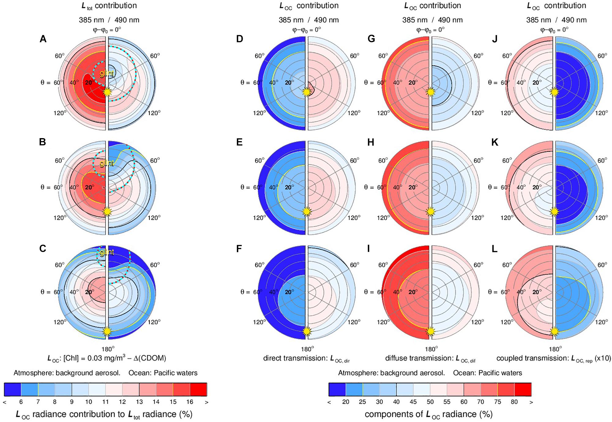
Figure 16. Radiative transfer simulations of radiance contributions to TOA observations. First column shows underwater light scattering radiance (LOC) contribution to TOA radiance (Ltot). Left and right hemispheres are for 385 and 490 nm, respectively. The sun (denoted by a yellow star in the backscattering direction) is located at 10° (first row), 30° (second row) and 50° (third row). Second, third and fourth columns show contributions to radiance (LOC) of direct transmitted water-leaving radiance (LOC,dir), diffuse transmitted radiance (LOC,dif), and coupled water-leaving radiance (LOC,rep), respectively.
where Latm(θ, φ) is the contribution of light scattered only in the atmosphere, Lsrf−atm(θ, φ) is the contribution of light scattered in the atmosphere and reflected (once or more times) by the ocean surface, and LOC is the ocean color contribution defined as light that has been scattered in the ocean body (but may also have been scattered in the atmosphere before entering, or after exiting, the ocean body). For simplicity, we will omit hereafter the dependence on θ and φ of radiance quantities and operators. To compute Latm, we used an efficient adding/doubling method described in detail by de Haan et al. (1987) for isolated atmospheres. We assumed for these computations a homogeneous atmosphere consisting of molecules (with optical thickness and depolarization ratio δm taken from Bodhaine et al., 1999) and a background fine-mode aerosol (with effective radius re = 0.1 μm as defined in Hansen and Travis, 1974; a spectrally constant refractive index m = 1.45; and optical thickness τaer = 0.10 at 550 nm). For the ocean surface in the computation of Lsrf−atm, we used the isotropic Gaussian surface slope distribution from Cox and Munk (1954) with surface wind speed U12.5 = 7 m/s, and included whitecaps with albedo Awc = 40% in the UV-A and VIS. To compute LOC, we used [Chla] = 0.03 mg/m3 as input for the D-P hydrosol model mentioned in Section “3.1.2 Bio-Optical Models” (see also Chowdhary et al., 2012), and adjusted the total underwater absorption coefficient atot to fit the anomalously low Kd values given by Morel et al. (2007a) for the South Pacific Gyre.
The plots in the first column of Figure 16 show (LOC/Ltot), i.e., they depict (see thin contour lines; given in percent of Ltot) the relative contribution to TOA radiance of light that has been scattered under water. Superimposed on these plots are outlines (see thick contour line; given at 10% level of Ltot − LOC) of the sunglint radiance contribution. There are several conclusions that can be drawn from these plots. Firstly, the underwater light scattering contribution can (at θ0 = 10°) become larger than 16% of the TOA radiance at 385 nm, whereas at 490 nm it remains less than 13% in spite of the atmosphere being optical thinner in the VIS (due to decrease in molecular scattering) than in the UV-A. The LOC contribution decreases at both wavelengths with increasing solar zenith angle, but it remains always larger at 385 nm than at 490 nm. This result differs from the one reported by Zhai et al. (2017a) – i.e., for the same [Chla] = 0.03, they report relative LOC contributions that are larger at 490 nm than at 385 nm for θ0 = 45°. The difference between our and their results can be attributed to variations in CDOM amount. That is, our and their underwater light absorption coefficients atot lead to diffuse attenuation coefficients Kd that (according to Figure 2 in Morel et al., 2007a) are typical for CDOM-poor Pacific Gyre waters and CDOM-rich Mediterranean waters, respectively. This comparison of RT results simply confirms (albeit for oligotrophic oceans) the sensitivity of UV-A radiance to retrieve variations in CDOM.
The first column of Figure 16 further shows that, regardless of CDOM amount, oligotrophic oceans can be sufficiently bright in the UV-A to contribute noticeable to the TOA radiance. This implies that any inversion algorithm that uses spaceborne UV-A radiance to constrain aerosol properties ωaer and Zaer (see discussion above on atmospheric correction) must also consider variations in ocean color that are caused by changes in [Chla] and/or CDOM. That may lead to challenging cases when inverting scenes that contain brown carbon (BrC) aerosols. Like CDOM (and unlike black carbon aerosols), BrC aerosols exhibit absorption spectra that increase rapidly toward the UV-A (Kirchstetter et al., 2004; Sun et al., 2007; Chen and Bond, 2010). Although the optical properties of CDOM and BrC particles vary in space and time, and although specifying their chemical structures remains an active field of research, CDOM and BrC have been associated with substances that have similar composition, i.e., marine humic matter (Boyle et al., 2009; Nelson and Siegel, 2013) and humic-like substances (HULIS) (Hoffer et al., 2006, 2016; George et al., 2015; Laskin et al., 2015), respectively. This may, at least in part, explain the similarity between CDOM and BrC absorption spectra. The ability to distinguish the impact on TOA radiance of such similarities in AOS absorption spectra is an outstanding question. Hence, retrieving ωaer (and Zaer) from spaceborne UV-A radiance observations over oceans is not always a trivial matter, and needs to be carefully examined in future studies.
The first column of Figure 16 also shows that the sunglint outline in Ltot becomes much smaller at 385 nm than at 490 nm. This is a direct result of the atmospheric optical depth becoming larger with decreasing wavelength, which causes the direct atmospheric attenuation of sunglint to decrease by a factor of up to two, and the diffuse atmospheric transmission to scatter the sunglint over a wider range of viewing angles. Furthermore, we found (not shown here) that when increasing the surface wind speed from 2 to 7 m/s, the sunglint outline in Ltot varies significantly less at 385 nm (spatial coverage changes by less than 10%) than at 490 nm (spatial coverage changes by up to 70%). That is because the diffuse transmission of sunglint through the atmosphere (i) contributes several factors more to the sunglint outline in Ltot at 385 nm than at 490 nm, and (ii) reduces the sensitivity of this glint to surface wind properties. The corresponding impact on the polarized component in Ltot remains to be studied, but will be of particular interest to spaceborne polarimetry of aerosols and hydrosols. That is, numerical studies show (see e.g., Chowdhary et al., 2006; Zhai et al., 2017b) that the polarized component Ltot becomes most sensitive to variations in underwater light scattering properties when approaching sunglint viewing angles for moderate to large solar zenith angles. Similar sensitivities can be expected for variations in aerosol scattering that in the UV-A will mostly perturb the large polarization of light scattered by molecules at 90°. However, the perturbations in UV-A polarized radiance caused by variations in aerosols and hydrosols will have different angular and spectral patterns (one of the reasons for this difference is the change in underwater light polarization pattern when this light crosses the ocean surface). Modern-age multi-angle and multi-spectral polarimeters such as SPEXone can distinguish such patterns with very high accuracies (i.e., with DoLP uncertainties <0.3%). This may offer a feasible pathway toward distinguishing variations caused by BrC aerosols and CDOM in the inversion of UV-A radiance (see discussion above on BrC aerosols).
We discussed above that the LOC radiance increases toward the UV-A for oligotrophic oceans. The LOC radiance itself can be further decomposed into several contributions that depend on the pathway of light taken through the atmosphere. Let LOC,dir and LOC,dif denote, respectively, the direct contribution (i.e., only attenuated by the atmosphere along the path to and from the ocean body) and the diffuse contribution (i.e., scattered in the atmosphere along the path to and/or from the ocean body) to LOC. Furthermore, let LOC,rep describe the residual contribution to LOC of light that has repeatedly interacted with the atmosphere and the ocean system (i.e., the system consisting of the ocean body and ocean surface). One can then write:
The plots in the second column of Figure 16 depict (LOC, dir/LOC), i.e., they show the contribution to LOC of underwater light that has never been scattered in the atmosphere. This contribution can be as large as 60% at 490 nm, but it decreases rapidly toward the UV-A where it is ≤30% at 385 nm. Hence most of the contribution to LOC in the UV-A has at some point been scattered in the atmosphere. The plots in the third column of Figure 16 depict (LOC, dif/LOC), and they show that the contribution to LOC in the UV-A comes mostly from LOC,dif. In the VIS, LOC,dif is often approximated by Gordon (1997) and Gao et al. (2007).
where L0 is the solar radiance illuminating the AOS, rwlr is a Lambertian reflector for water-leaving radiance, and eτ/μ and tatm are the scalar direct and diffuse transmittance factors for the atmosphere, respectively. Here, τ is the optical thickness of the atmosphere, and μ0 and μ are the cosine of the sun and viewing angles, respectively. Hence rwlr ignores the facts that the water-leaving radiance is bidirectional (Morel and Gentili, 1993; Morel et al., 2002; Fan et al., 2015) and highly polarized (Chowdhary et al., 2006; Tonizzo et al., 2011; Zhai et al., 2017b). Furthermore tatm ignores the impact of polarization (not just of light in the atmosphere but also of water-leaving radiance) on RT computations for the atmosphere, which can lead to substantial errors in transmitted radiance (Lacis et al., 1998). Some inversion methods go a step further by modifying the direct transmittance factor eτ/μ to include tatm (Gordon et al., 1983; Gordon (1997)), and by inserting empirically derived coefficients to improve the accuracy of such modifications (Wang, 1999). Given the dominant contribution of LOC,dif to LOC in the UV-A, such approximations need to be re-examined and evaluated against PACE’s accuracy requirements (cf. “1.1 The PACE Mission” section, see also NASA, 2018a) for retrievals of LOC.
The fourth column of Figure 16 shows plots of (LOC, rep/LOC). Note that the values in these plots, which describe the contribution to LOC of light that is repeatedly reflected between the atmosphere and ocean system, are multiplied by a factor of 10 to magnify their magnitude. This light contributes (much) less than 4% to LOC at 490 nm because of the low albedo of the ocean and of the atmosphere at this wavelength. Some inversion methods for LOC radiance therefore ignore this contribution altogether in the VIS (e.g., Gordon et al., 1983; Gordon, 1997; Wang, 1999). Other inversion methods still include this contribution albeit only for light that is transmitted (not reflected) back and forth by the ocean surface (e.g., Gao et al., 2000, 2007, 2009). At 385 nm, radiance LOC, rep increases in absolute terms by a factor of more 50 when compared to its absolute value at 490 nm (not shown here). From Figure 16, we see that LOC, rep now contributes up to 7% to LOC. This contribution originates from a complex coupling of light scattered by the atmosphere and ocean system, e.g., it includes water-leaving radiance that is scattered by the atmosphere back to the ocean surface and that is subsequently reflected back to sky by this surface. This coupling cannot be simplified even when using a Lambertian reflector rwlr for water-leaving radiance. Therefore any inversion algorithm that uses spaceborne UV-A radiance to simultaneously retrieve aerosol and ocean properties (see, e.g., previous discussion on constraining BrC aerosol and CDOM over oligotrophic waters) must also consider truly coupled atmosphere-ocean systems if LOC, rep is deemed too large to ignore. Note that LOC, rep will decrease in magnitude if [Chla] or CDOM increases (which darkens the ocean in the UV), or if the amount of back-scattering in the atmosphere decreases (e.g., because of a change in aerosol properties). On the other hand, the vicinity of bright surfaces in the UV-A such as sea ice or snow-covered land will not only exuberate adjacency effects that were discussed in the Section “3.4.2 Horizontal Variations,” but will also increase in particular LOC, rep radiance because of repeated skylight reflections off such surfaces.
This paper summarizes research frontiers on RT in coupled ocean and atmosphere systems to enable new ocean-atmosphere science and specifically to support the PACE mission development. RT is an essential tool in remote sensing of atmosphere and ocean components, and in furthering our understanding of the coupled system. It is used to facilitate designing new retrieval algorithms; providing validation datasets for satellite data products; and performing sensitivity to different components of the Earth system. In anticipation of the advanced remote sensing capabilities of the instruments onboard the PACE spacecraft, the PACE Science Team has performed novel FWD RT and INV RT studies on different components of the atmosphere-ocean system. This work included examining the representation of hydrosols, aerosols, gases, surface whitecaps and sunglint in these models. In addition, bio-optical models, the key element in practical RT for ocean applications, were investigated from several perspectives. The team also has evaluated fundamental processes and assumptions of common RT models including inelastic scattering, and 3D effects such as spherical shells and adjacency effects. This has resulted in a set of calculations from state-of-the-art RT models that have been published to serve as a benchmark for future coupled ocean and atmosphere RT applications.
To better represent hydrosol optical properties in RT, Chowdhary, Liu et al. (unpublished) have studied the impacts of particle shape and inhomogeneity on scattering matrices of hydrosols. Their study suggests that internal structures of plankton-like particles need to be considered when using RT computations to analyze backscattering radiance. Furthermore, they suggest that there is information content on plankton morphology in ocean depth profiles of depolarization ratios δL obtained from air- and space-borne lidars. On modeling the phase function of hydrosols, Twardowski et al. (unpublished) have used a linear combination of two cluster representations, which has been verified by a large collection of volume scattering function measurements. This method can show an improvement of RMS errors of several percent relative to Fournier-Forand phase functions when considering the full VSF angular range, but, unlike the latter function, has no physical meaning. The phase function of hydrosols in the backward directions, as shown recently by Zhang et al. (2017), can be approximated by a linear combination of two end members, one representing the scattering by particles of sizes much smaller than the wavelength of light and the other by particles of sizes much greater than the wavelength of light.
Another approach to analyze measured hydrosol phase functions was taken by Zhang et al. (2011) and Twardowski et al. (2012) who computed an extensive library of optically unique phase functions that serve as fingerprints for various oceanic particle species. Each particle species represented by this library has its own refractive index and its own log-normal size distribution, both of which were determined through sensitivity analyses over the ranges of published size distributions and composition for oceanic particles. In Zhang et al. (2011) the particle species are assumed spherical, whereas in Twardowski et al. (2012) the particles assume non-spherical shapes consisting of asymmetrical hexahedra for inorganic mineral particles (Bi et al., 2010). Both studies used coated spheres (Czerski et al., 2011; Zhang et al., 2011) to represent air bubbles. This library of phase functions has subsequently been used to invert measured hydrosol phase functions into the scattering coefficient and size distribution of particle subpopulations (Twardowski et al., 2012; Zhang et al., 2012, 2013, 2014b).
We note at this point that while each of the above-mentioned approaches for hydrosol scattering (i.e., internal structure of plankton, non-spherical shape of marine particulates, submicron-sized marine particulates, VSF decomposition) may provide a reasonable or partial solution for the “missing particulate backscattering enigma” (see discussions in Stramski et al., 2004; Organelli et al., 2018; Poulin et al., 2018), a particle model that incorporates all these approaches to study their combined impact on backscattering remains an outstanding topic of research. Such a model could validate, or lead to adjustments of, parameter choices made for each approach such as refractive index and shape distributions of marine particles. We anticipate that further measurement and experimentation with VSFs including underwater light polarization and lidar depolarization measurements will provide additional information to help constrain, and perhaps even reduce, the parameters of such a complex model. Emerging particle characterization methods such as in situ holographic imaging (Talapatra et al., 2013; Nayak et al., 2017) are also expected to aid in development and validation of such a model.
Unlike hydrosols and aerosols, the absorption properties of gases are well known. The advances reported in this work concern expanding the representation of gaseous absorption in RT modeling in a practical sense to high spectral resolution across the full solar spectrum. At NASA’s OBPG, and as part of the PACE ST activities, a hyperspectral atmospheric correction algorithm was developed, based on the well-established heritage algorithm in combination with the ATREM algorithm for gas correction, to derive the hyperspectral water-leaving reflectance from airborne and spaceborne hyperspectral sensors. The AC algorithm was tested and validated using HICO data as a proxy for anticipated OCI observations. The results show the consistency and feasibility of the hyperspectral AC process including the gas absorption correction (Ibrahim et al., 2018). However, several gaps in the RT developments still exist, such as modeling efficiently the fine absorption features of water vapor and Oxygen, and the coupling between gas absorption features and molecular and aerosol scattering. The development of such capabilities will be needed to fully utilize OCI’s hyperspectral coverage, such as the Oxygen A-band for the aerosol layer height and the plankton fluorescence retrieval.
The PACE Science Team also investigated the reflectance of whitecaps due to wave breaking, and how to represent this reflectance in RT. New spectral measurements of whitecaps have been made across from 400 to 2500 nm (Dierssen, 2019). These measurements show that whitecaps reflectances have spectral dips in the NIR spectrum that largely correspond to the absorption features of liquid water. Reflectance dips occur particularly at 750, 980, and 1150 nm, which have enhanced liquid water absorption, a result of multiple scattering in and around subsurface bubbles and surface foam. Following Whitlock et al. (1982), a simple model of whitecap reflectance based on the natural logarithm of water absorption can be used to describe the spectral shape of intense whitecaps generated by breaking waves into SWIR wavelengths. Moreover, the decrease in reflectance at these liquid water absorption bands is correlated with enhancements in reflectance of the whitecap across the spectrum. The conclusion drawn by this PACE Science Team is that current models based on wind speed and a single whitecap albedo cannot be used to accurately represent the diversity of whitecaps on the ocean.
Another RT topic that was reexamined by the PACE team is the information contained in sunglint observations. Obtaining that information requires vector RT with polarization. In the SWIR (where the interaction of light with the atmosphere and ocean body is minimized) the DoLP within sunglint is only sensitive to the ocean surface refractive index, m. Variations in m occur throughout the global ocean for large changes in sea surface temperature and salinity, but also in the presence of substances covering the ocean surface such as slicks from biogenic origin (e.g., plankton and fish secretions) and anthropogenic origin (e.g., oil spills). An intriguing application involves the detection of variations in the uppermost 1–1000 μm of the ocean, which is referred to as the surface microlayer and which has biological, chemical, and physical properties that are distinctively different from those of the underlying ocean body. Ottaviani et al. (2019) developed an inversion algorithm to provide continuous (i.e., along aircraft ground track) retrievals of m from airborne sunglint DoLP observations by the RSP instrument at 2.2 μm. They demonstrate that the multi-angle views and high DoLP accuracy of RSP measurements allows m to be retrieved within 5 × 10⁻⁴ under ideal experimental conditions. Actual retrieval examples are shown for pristine sea surfaces and the Deepwater Horizon oil spill.
In ocean color remote sensing, bio-optical models are needed to correlate water leaving radiance at different wavelengths. The correlation occurs by means of prescribing variations in the magnitude and spectra of IOPs. For traditional “Case I” waters, one can – to a first order approximation – parameterize IOPs in terms of the Chlorophyll a concentration [Chla]. This is a strong constraint though, which often fails in coastal waters. Considerable efforts have been made to relax the dependence of IOPs on [Chla] (Werdell et al., 2013a). However, bio-optical models developed for analyzing polarized water-leaving radiance spectra still use [Chla] to parameterize IOPs (Chowdhary et al., 2006; Zhai et al., 2010; Hasekamp et al., 2011; Xu et al., 2016). Chowdhary, Stamnes et al. (unpublished) have taken the next step in developing the Detritus-Plankton (D-P) II hydrosol model, where the backscattering coefficient for particulate matter and absorption coefficient for colored detrital matter are allowed to vary independently of [Chla]. More than 1.7 million reflection matrices for water-leaving radiance were computed with this model, and are now available at https://data.giss.nasa.gov/rad/ocean-matrices/. These matrices are currently used to analyze airborne polarimetric (RSP) and lidar (HSRL) data obtained during the 2012 TCAP and the 2014 SABOR campaign (Stamnes et al., 2018), and the ongoing NAAMES campaign. In addition, Ibrahim et al. (2016) and Zhai et al. (2017b) have adopted a bio-optical model that added sediment concentration to parameterize IOPs. This philosophy has been adopted to design an inversion algorithm that retrieves aerosol and hydrosol parameters simultaneously (Gao et al., 2018).
In addition to extending the number of parameters used to prescribe variations in IOPs for analyses of polarized water-leaving radiance, the PACE Science Team also extended the spectral range in prescribed IOP variations for analyses of total water-leaving radiance. Specifically, the IOCCG Report 5 (IOCCG-OCAG, 2003; IOCCG, 2006) prescribed variations in IOPs from 400 to 800 nm, and created synthetic data sets to test the performance of IOPs inversion algorithms. This spectral range has now been extended down to 350 nm to produce synthetic data sets for UV-A radiance from PACE/OCI. In addition, wider variations are now adopted for phytoplankton absorption spectra aph (using a larger range at 440 nm, and more normalized spectral shapes) to cover oceans ranging from oligotrophic to waters with plankton blooms. Updates are also made in the absorption coefficient aw for pure sea water based on the work by Lee et al. (2015), and in the backscattering coefficient bb,w for pure sea water based following Zhang et al. (2009). Finally, slightly different variations with [Chla] (compared to the parameterizations in IOCCG (2006) are now used for the attenuation coefficient cph and the scattering coefficient bd,m for phytoplankton and non-algae particulate matter, respectively, at 550 nm.
Radiative transfer simulations for the atmosphere and for the ocean have prioritized the modeling of different phenomena. Atmospheric modeling almost always includes polarization but rarely inelastic scattering, while ocean RT modeling often ignores polarization, but does address inelastic scattering. At the onset of the PACE Science Team in 2015, no coupled ocean-atmosphere RT model that addressed both polarization and inelastic scattering in the ocean could be identified. Since then, Zhai et al. (2015, 2017a) have developed a RT model based on the successive order of scattering method that can accurately handle polarization, atmosphere and ocean coupling, elastic and inelastic scattering. The inelastic scattering mechanisms include Raman scattering due to ocean waters, fluorescent dissolved organic matter, and fluorescence by chlorophyll. Furthermore, the photochemical and NPQ processes of the chlorophyll fluorescence have been accounted for in Zhai et al. (2018). The RT model has been used to study the sensitivity of TOA polarized radiance to contributions originating from underwater light scattering in open and coastal ocean waters, which can be used to design new atmospheric correction algorithms (Zhai et al., 2017b).
Another common omission in RT is Earth curvature that may affect significantly the TOA signal, not only at large solar zenith and viewing angles, but also at small viewing angle. It needs to be taken to account in RT simulations for accurate water reflectance retrievals, especially at high latitudes. Two processes are essentially at play in a spherical-shell atmosphere: 1) reduced illumination volume and 2) reduced attenuation of the downward solar beam. The earth curvature effect at low viewing angle has been largely ignored, since it is relatively small compared with the effect at large viewing angle, but neglecting it may not yield the rather demanding accuracy required for PACE science objectives. Pseudo-spherical corrections (e.g., just accounting for air mass change in the incident solar beam) may be sufficient at large solar zenith angle, but they do not capture effects at low viewing angle. Monte Carlo codes operated in backward mode are tools of predilection to quantify “exactly” spherical effects and generate look-up tables (e.g., molecule and aerosol scattering) for atmospheric correction algorithms. Adjacency effects due to the proximity of land, sea ice, or clouds, on the other hand, can be felt at relatively far distances (>10 km), their magnitude depending on the contrast between the reflectance of the target and its surroundings and the optical thickness of the atmosphere. Monte Carlo codes allow simulations for any spatial heterogeneity configuration; they offer a great deal of flexibility. Impacts on TOA measurements are calculated precisely, as well as the atmospheric spread function, which can be used in efficient corrective schemes, allowing image processing in the usual “large target” RT formalism.
Because of the wide variety of ocean, atmosphere and coupled RT models in current use, each with their own representation of optically active components and their own set of assumptions, there is a spread of solutions resulting from these models. We require a set of calculations, agreed upon by multiple RT codes to set a benchmark for future RT results for the ocean and atmosphere coupled system. In the PACE Science Team, a set of typical ocean and atmosphere coupled systems have been designed to perform polarized RT simulations. Several RT models have been used to perform the simulations and the inter-comparison has led to 25,000+ RT results with an accuracy ranging between 10−5 and 10−6 in terms of reflectance (Chowdhary et al., “Benchmark results for scalar and vector radiative transfer computations of light in atmosphere-ocean systems”, unpublished). This benchmark has exceeded any previous dataset for the coupled ocean and atmosphere system.
Despite the advances described above, gaps remain in RT topics that require continued research in the near future. Several topics were identified by the PACE Science Team:
• For RT of light in the ocean, these topics are (i) better understanding of the role of absorption by dissolved inorganics in the UV (FWD RT studies); (ii) better understanding of variability in backscattering shape of VSF (FWD and INV RT studies); (iii) developing particulate models that combine non-sphericity and inhomogeneity (FWD and INV RT studies); (iv) accounting for temperature and salinity dependence of Raman scattering and emission (FWD RT studies).
• For ocean surface reflection, outstanding topics are (i) impact of anisotropic surface roughness on the reflection of diffuse skylight (FWD RT studies); (ii) polarization properties of whitecaps in the UV-SWIR (FWD RT studies).
• For RT of light in the atmosphere, more research is needed on (i) retrieving multiple aerosol species that within a given size mode co-exist as external or internal mixtures (INV RT studies); (ii) characterizing aerosol properties in the UV (INV RT studies); (iii) retrieving aerosol vertical distribution from UV polarimetry (INV RT studies).
• For UV remote sensing of AOS, attention should be given to (i) approximations made for the coupling of atmosphere and ocean (FWD RT studies); (ii) accounting for simultaneous variations in absorbing aerosols and absorbing oceanic matter (INV RT studies); (iii) accounting for short-term variations of solar irradiance (INV RT studies).
This list, which is not all-inclusive, should be viewed within the context of advancement of accuracies in FWD and INV RT modeling for ensuring the fidelity to nature and/or meeting the radiometric (NASA, 2018a) and polarimetric (NASA, 2018b) measurement targets and products for PACE. Development of new technologies with subsequent experimentation will be required to address many of these gaps. Note that PACE data and products will serve many communities, and that these communities participate in research of interdisciplinary fields. Hence it is not possible to assign an order of importance to the above-mentioned topics. Furthermore, both numerical accuracy and efficiency are major concerns for making advances in INV RT modeling. Depending on the information content contained in an instrument with specific combinations of spectral, angular and polarimetric measurements and uncertainties, one often needs to makes trade-offs between accuracy and efficiency by considering approximation. So the development of retrieval oriented RT modeling approaches is another task for ocean color remote sensing and should be done in the next stage.
Overall, we conclude that RT modeling of multi-spectral polarized light in atmosphere-ocean systems has made significant forward progress during the tenure of the first PACE Science Team. While there are facets that will require further development to meet the capabilities required of the PACE and other missions, and to push ocean and atmospheric science forward, we are confident that the new results presented here will help both the atmosphere and ocean color communities make progress to meet these challenges. In addition, we strongly encourage these communities to view their challenges as a coupled problem, affecting both ocean and atmosphere that can only be met by working together. Thus, coupled science and effort must go hand-in-hand with improved coupled RT modeling. This is an essential step toward approaching the focus questions that are posed in the Aerosol-Ocean Interactions science traceability matrix (STM) for Aerosols, Cloud and Ecosystem (ACE) (Behrenfeld and Meskhidze, 2017), and solving some of the most pressing problems threatening the sustainability of our planet.
Jacek Chowdhary, Emmanuel Boss, Heidi Dierssen, Robert Frouin, Amir Ibrahim, Zhongping Lee, Lorraine Remer, Michael Twardowski, Feng Xu and Xiaodong Zhang.
JC and P-WZ were responsible for the overall structure and flow of the manuscript. JC was a co-lead author for sections “Introduction,” “The PACE Mission,” “Complexity of Atmosphere-Ocean Systems,” “History of RT Methods for OAS: A Brief Overview,” “Current RT Topics and Models: Heritage Studies, Discussion, and PACE Updates,” “Ocean Body,” “Particulate Scattering,” “Bio-Optical Models,” “Sunglint,” “Aerosols,” “RT Validations,” “Horizontal Variations,” and “UV Remote Sensing of AOS.” P-WZ was a co-lead author for sections “Introduction,” “The PACE Mission,” “Complexity of Atmosphere-Ocean Systems,” “History of RT Methods for OAS: A Brief Overview,” “Inelastic Scattering,” “Gases,” and “RT Validations.” EB was a co-lead author for sections “Bio-Optical Models” and “Molecular Scattering.” HD was a co-lead author for section “Whitecaps.” RF was a co-lead author for section “Horizontal Variations.” AI was a co-lead author for section “Gases.” MT was a co-lead author for sections “Particulate Scattering” and “Molecular Scattering.” MO was a co-lead author for section “Sunglint.” LAR was a co-lead author for section “Aerosols.” ZL was a co-lead author for sections “Particulate Scattering” and “Bio-Optical Models.” FX was a co-lead author for section “RT Validations.” XZ was a co-lead author for section “Particulate Scattering.” DR contributed to section “Horizontal Variations.” WRE contributed to section “Aerosols.” All authors contributed to section “Concluding Remarks” and approved the submitted version of the manuscript.
This work was supported by NASA Grant NNH13ZDA001N-PACEST. In addition, P-WZ was partially supported by additional funds from the NASA PACE Project and also acknowledged support by NASA Grants (NNX15AB94G and 80NSSC18K0345). MT further acknowledged additional support from the HBOI Foundation, and XZ from NASA (NNX13AN72G and 0NSSC17K0656) and from NSF (1355466 and 1459168).
The authors declare that the research was conducted in the absence of any commercial or financial relationships that could be construed as a potential conflict of interest.
The authors thank the reviewers for their constructive comments on an earlier version of this manuscript, and greatly appreciate the discussions with Otto Hasekamp and Jeremy Werdell on specifics of the PACE mission, and the discussions with Ziauddin Ahmad, Brian Cairns, and Bo-Cai Gao on UV-A solar spectra.
Aas, E. (1996). Refractive index of phytoplankton derived from its metabolite composition. J. Plankton Res. 18, 2223–2249. doi: 10.1093/plankt/18.12.2223
Adams, C. D., and Kattawar, G. W. (1978). Radiative transfer in spherical shell atmospheres I. Rayleigh scattering. Icarus 35, 139–151. doi: 10.1016/0019-1035(78)90067-2
Adams, C. N., and Kattawar, G. W. (1993). Effect of volume-scattering function on the errors induced when polarization is neglected in radiance calculations in an atmosphere-ocean system. Appl. Opt. 32, 4610–4617.
Adams, J. T., and Kattawar, G. W. (1997). Neutral points in an atmosphere–ocean system. 1: upwelling light field. Appl. Opt. 36, 1976–1986.
Ahmad, Z., Franz, B. A., McClain, C. R., Kwiatkowska, E. J., Werdell, J., Shettle, E. P., et al. (2010). New aerosol models for the retrieval of aerosol optical thickness and normalized water-leaving radiances from the SeaWiFS and MODIS sensors over coastal regions and open oceans. Appl. Opt. 49:5545. doi: 10.1364/AO.49.005545
Ahmad, Z., and Fraser, R. S. (1982). An iterative transfer code for atmosphere-ocean systems. J. Atm. Sci. 39, 656–665. doi: 10.1175/1520-0469(1982)039<0656:airtcf>2.0.co;2
Ahmad, Z., Mc Clain, C. R., Herman, J. R., Franz, B. A., Kwiatkowska, E., Robinson, W. D., et al. (2007). Atmospheric correction for NO2 absorption in retrieving water-leaving reflectances from the SeaWiFS and MODIS measurements. Appl. Opt. 46, 6504–6512.
Anderson, G., Clough, S., Kneizys, F., Chetwynd, J., and Shettle, E. (1986). AFGL Atmospheric Constituent Profiles (0 - 120 Km), 1-TR-86-0110. Hanscom AFB, MA: U.S. Air Force Geophysics Laboratory. Optical Physics Division.
Antonov, J. I., Seidov, D., Boyer, T. P., Locarnini, R. A., Mishonov, A. V., Garcia, H. E., et al. (2010). “World ocean atlas 2009, volume 2: salinity,” in NOAA NESDIS 68, ed. S. Levitus (Washington, DC: U.S. Government PrintingOffice), 39.
Armstrong, F. A. J., and Boalch, G. T. (1961). The ultra-violet absorption of sea water. J. Mar. Biol. Assoc. 41, 591–597.
Artlett, C. P., and Pask, H. M. (2015). Optical remote sensing of water temperature using Raman spectroscopy. Opt. Express 23, 31844–31856. doi: 10.1364/OE.23.031844
Artlett, C. P., and Pask, H. M. (2017). New approach to remote sensing of temperature and salinity in natural water samples. Opt. Express 25, 2840–2851. doi: 10.1364/OE.25.002840
Baker, A. R., Laskina, O., and Grassian, V. H. (2014). “Processing and ageing in the atmosphere, in mineral dust,” in A Key Player in the Earth System, eds P. Knippertz and J.-B. W. Stuut (Berlin: Springer), 75–92. doi: 10.1007/978-94-017-8978-3_4
Balch, W. M., Vaughn, J. M., Drapeau, D. T., Bowler, B. C., Booth, E., Vining, C. L., et al. (2004). “Case I/II ambiguities in algal blooms: the case for minerals and viruses,” in Proceedings of the American Society of Limnology and Oceanography/The Oceanography Society, Ocean Research 2004 Conference, (Honolulu).
Baran, A. J., and Labonnote, L. C. (2006). On the reflection and polarization properties of ice clouds. J. Quant. Spectrosc. Radiat. Transf. 100, 41–54.
Barnes, W. L., Pagano, T. S., and Salomonson, V. V. (1998). Prelaunch characteristics of the moderate resolution imaging spectroradiometer (MODIS). on EOS-AM1. IEEE Trans. Geosci. Remote Sens. 36, 1088–1100. doi: 10.1109/36.700993
Bauer, S. E., Tsigaridis, K., and Miller, R. L. (2016). Significant atmospheric aerosol pollution caused by world food cultivation. Geophys. Res. Lett. 43, 5394–5400. doi: 10.1002/2016GL068354
Behrenfeld, M., and Meskhidze, N. (2017). Response to the 2017 NRC Decadal Survey Request for Information Regarding the OCEAN ECOSYSTEM and OCEAN-AEROSOL INTERACTIONS Components of the Aerosol, Cloud, and Ocean Ecosystem (ACE). Mission. Available at: https://acemission.gsfc.nasa.gov/documents/whitepapers/RFI-2c%20Ocean.pdf. doi: 10.1002/2016gl068354 (accessed May 11, 2019).
Behrenfeld, M. J., Bale, A. J., Kolber, Z. S., Aiken, J., and Falkowski, P. G. (1996). Confirmation of iron limitation of phytoplankton photosynthesis in the equatorial Pacific ocean. Nature 383, 508–511. doi: 10.1038/383508a0
Behrenfeld, M. J., and Kolber, Z. S. (1999). Widespread iron limitation of phytoplankton in the South Pacific Ocean. Science 283, 840–884.
Behrenfeld, M. J., Westberry, T. K., Boss, E. S., O’Malley, R. T., Siegel, D. A., Wiggert, J. D., et al. (2009). Satellite-detected fluorescence reveals global physiology of ocean phytoplankton. Biogeosciences 6, 779–794. doi: 10.5194/bg-6-779-2009
Bellouin, N., Boucher, O., Tanré, D., and Dubovik, O. (2003). Aerosol absorption over the clear-sky oceans deduced from POLDER-1 and AERONET observations. Geophys. Res. Lett. 30:1748.
Bergametti, G., and Forêt, G. (2014). “Dust deposition, in mineral dust,” in A Key Player in the Earth System, eds P. Knippertz and J.-B. W. Stuut (Berlin: Springer), 179–196.
Bernard, S., Probyn, T. A., and Quiantes, A. (2009). Simulating the optical properties of phytoplankton cells using a two-layered spherical geometry. Biogeosci. Discuss. 6, 1497–1563. doi: 10.5194/bgd-6-1497-2009
Bi, L., and Yang, P. (2015). Impact of calcification state on the inherent optical properties of coccoliths and coccolithophores. J. Quant. Spectrosc. Radiat. Transf. 155, 10–21. doi: 10.1016/j.jqsrt.2014.12.017
Bi, L., Yang, P., Kattawar, G. W., and Kahn, R. (2010). Modeling optical properties of mineral aerosol particles by using nonsymmetric hexahedra. Appl. Opt. 49, 334–342. doi: 10.1364/AO.49.000334
Bishop, J. K., Davis, R. E., and Sherman, J. T. (2002). Robotic observations of dust storm enhancement of Carbon biomass in the North Pacific. Science 298, 817–821. doi: 10.1126/science.1074961
Blondeau-Patissier, D., Gower, J. F. R., Dekker, A. G., Phinn, S. R., and Brando, V. E. (2014). A review of ocean color remote sensing methods and statistical techniques for the detection, mapping and analysis of phytoplankton blooms in coastal and open oceans. Progr. Oceanogr. 123, 123–144. doi: 10.1016/j.pocean.2013.12.008
Bodhaine, B. A., Wood, N. B., Dutton, E. G., and Slusser, J. R. (1999). On rayleigh optical depth calculations. J. Atmos. Ocean. Technol. 16, 1854–1861. doi: 10.1175/1520-0426(1999)016<1854:orodc>2.0.co;2
Bogumil, K., Orphal, J., Homann, T., Voigt, S., Spietz, P., Fleischmann, O. C., et al. (2003). Measurements of molecular absorption spectra with the SCIAMACHY pre-flight model: instrument characterization and reference data for atmospheric remote-sensing in the 230–2380 nm region. J. Photochem. Photobiol. A 157, 167–184. doi: 10.1016/s1010-6030(03)00062-5
Bohren, C., and Huffman, D. (1983). Absorption and Scattering of Light by Small Particles. New York, NY: Wiley.
Born, M., and Wolf, E. (1999). Principles of Optics. Electromagnetic Theory of Propagation, Interference and Diffraction of Light. Cambridge: Cambridge University Press.
Boss, E., and Pegau, W. S. (2001). Relationship of light scattering at an angle in the backward direction to the backscattering coefficient. Appl. Opt. 40, 5503–5507.
Bouffiès, S., Bréon, F. M., Tanré, D., and Dubuisson, P. (1997). Atmospheric water vapor estimate by a differential absorption technique with the polarisation and directionality of the Earth reflectances (POLDER). instrument. J. Geophys. Res. 102, 3831–3841. doi: 10.1029/96JD03126
Boyd, P. W., Mackie, D. S., and Hunter, K. A. (2009). Aerosol iron deposition to the surface ocean – Modes of iron supply and biological responses. Mar. Chem. 10, 128–143. doi: 10.1016/j.marchem.2009.01.008
Boyd, P. W., Watson, A. J., Law, C. S., Abraham, E. R., Trull, T., Murdoch, R., et al. (2000). A mesoscale phytoplankton bloom in the polar southern ocean stimulated by iron fertilization. Nature 407, 695–702. doi: 10.1038/35037500
Boyle, E. S., Guerriero, N., Thiallet, A., Del Vecchio, R., and Blough, N. V. (2009). Optical properties of humic substances and CDOM: relation to structure. Environ. Sci. Technol. 43, 2262–2268. doi: 10.1021/es803264g
Bréon, F. M., and Doutriaux-Boucher, M. (2005). A comparison of cloud droplet radii measured from space. IEEE Trans Geosci. Remote Sens. 43, 1796–1805. doi: 10.1109/tgrs.2005.852838
Bréon, F.-M., and Goloub, P. (1998). Cloud droplet effective radius from spaceborne polarization measurements. Geophys. Res Lett. 25, 1879–1882. doi: 10.1029/98gl01221
Bréon, F. M., and Henriot, N. (2006). Spaceborne observations of ocean glint reflectance and modeling of wave slope distributions. J. Geophys. Res. 11:C06005. doi: 10.1029/2005JC003343
Bricaud, A., Babin, M., Morel, A., and Claustre, H. (1995). Variability in the chlorophyll-specific absorption coefficients of natural phytoplankton: analyses and parameterization. J. Geophys. Res. 100, 13321–13332.
Bricaud, A., Morel, A., Babib, M., Allali, K., and Claustre, H. (1999). Erratum: variations of light absorption by suspended particles with chlorophyll a concentrations in oceanic (case 1). waters: analysis and implications for bio-optical models. J. Geophys. Res. 104:8025. doi: 10.1029/1999jc900030
Bricaud, A., Morel, M., Babin, M., Allali, K., and Claustre, H. (1998). Variations of light absorption by suspended particles with Chlorophyll a concentration in oceanic (case 1). Waters: analyses and implications for bio-optical models. J. Geophys. Res. 103, 31033–31044. doi: 10.1029/98jc02712
Brumer, S. E., Zappa, C. J., Brooks, I. M., Tamura, H., Brown, S. M., Blomquist, B. W., et al. (2017). Whitecap coverage dependence on wind and wave statistics as observed during SO GasEx and HiWinGS. J. Phys. Oceanogr. 47, 2211–2235. doi: 10.1175/jpo-d-17-0005.1
Buehler, S. A., Eriksson, P., and Lemke, O. (2011). Absorption lookup tables in the radiative transfer model ARTS. J. Quant. Spectrosc. Radiat. Transf. 112, 1559–1567. doi: 10.1016/j.jqsrt.2011.03.008
Buiteveld, H., Hakvoort, J. H. M., and Donze, M. (1994). The optical properties of pure water. SPIE Ocean Optics XII 2258, 174–183.
Bulgarelli, B., and Doyle, J. P. (2004). Comparison between numerical models for radiative transfer simulation in the atmosphere-ocean system. J. Quant. Spectrosc. Radiat. Transf. 86, 315–334. doi: 10.1016/j.jqsrt.2003.08.009
Burrows, S. M., Ogunro, O., Frossard, A. A., Russell, L. M., Rasch, P. J., and Elliot, S. M. (2014). A physically-based framework for modelling the organic fractionation of sea spray aerosol from bubble film Langmuir equilibria. Atmos. Chem. Phys. Discuss. 14, 5375–5443. doi: 10.5194/acpd-14-5375-2014
Cairns, B., Russell, E. E., LaVeigne, J. D., and Tennant, P. M. W. (2003). “Research scanning polarimeter and airborne usage for remote sensing of aerosols,” in Proceedings of the Polarization Science and Remote Sensing, (San Diego, CA).
Cairns, B., Russell, E. E., and Travis, L. D. (1999). The research scanning polarimeter: calibration and ground-based measurements. Proc. SPIE 3754, 186–197.
Carder, K. L., Chen, F. R., Lee, Z. P., Hawes, S., and Kamykowski, D. (1999). Semi-analytic MODIS algorithms for chlorophyll a and absorption with bio-optical domains based on nitrate-depletion temperatures. J. Geophys. Res. 104, 5403–5421. doi: 10.1029/1998jc900082
Carnesecchi, F., Byfield, V., Cipollini, P., Corsini, G., and Diani, M. (2008). “An optical model for the interpretation of remotely sensed multispectral images of oil spill,” in Proceedings of the Remote Sensing of the Ocean, Sea Ice, and Large Water Regions, (San Diego, CA).
Carslaw, K. S., Boucher, O., Spracklen, D. V., Mann, G. W., Rae, J. G. L., Woodward, S., et al. (2010). A review of natural aerosol interactions and feedbacks within the Earth system. Atmos. Chem. Phys. 10, 1701–1737. doi: 10.5194/acp-10-1701-2010
Caudill, T. R., Flitter, D. E., and Herman, B. M. (1997). Evaluation of the pseudo-spherical approximation for backscattered ultraviolet radiances and ozone retrieval. J. Geophys. Res. 102, 3881–3890. doi: 10.1029/96jd03266
Chami, M., Lafrance, B., Fougnie, B., Chowdhary, J., Harmel, T., and Waquet, F. (2015). OSOAA: a vector radiative transfer model of coupled atmosphere-ocean system for a rough sea surface application to the estimates of the directional variations of the water leaving reflectance to better process multi-angular satellite sensors data over the ocean. Opt. Express 23, 27829–27852. doi: 10.1364/OE.23.027829
Chami, M., Santer, R., and Dillegeard, E. (2001). Radiative transfer model for the computation of radiance and polarization in an atmosphere-ocean system: polarization properties of suspended matter for remote sensing. Appl. Opt. 40, 2398–2416.
Chen, Y., and Bond, T. C. (2010). Light absorption by organic carbon from wood combustion. Atmos. Chem. Phys. 10, 1773–1787. doi: 10.5194/acp-10-1773-2010
Chepfer, H., Goloub, P., Reidi, J., De Haan, J., Hovenier, J., and Flamant, P. H. (2001). Ice crystal shapes in cirrus clouds derived from POLDER-1/ADEOS-1. J. Geophys. Res. Atmos. 106, 7955–7966. doi: 10.1029/2000jd900285
Chesters, D., Uccellini, L. W., and Robinson, W. D. (1983). Low-level water vapor fields from the VISSR atmospheric sounder (VAS). split window channels. J. Clim. Appl. Meteorol. 22, 725–743. doi: 10.1175/1520-0450(1983)022<0725:llwvff>2.0.co;2
Chowdhary, J., Cairns, B., Mishchenko, M. I., Hobbs, P. V., Cota, G. F., Redemann, J., et al. (2005). Retrieval of aerosol scattering and absorption properties from photopolarimetric observations over the ocean during the CLAMS experiment. J. Atmos. Sci. 62, 1093–1117. doi: 10.1175/jas3389.1
Chowdhary, J., Cairns, B., Mishchenko, M. I., and Travis, L. D. (2001). Retrieval of aerosol properties over the ocean using multispectral and multiangle photopolarimetric measurements from the Research Scanning Polarimeter. Geophys. Res. Lett. 28, 234–246.
Chowdhary, J., Cairns, B., and Travis, L. (2002). Case studies of aerosol retrievals from multi-angle, multi-spectral photo-polarimetric remote sensing data. J. Atmos. Sci. 59, 383–397.
Chowdhary, J., Cairns, B., and Travis, L. D. (2006). Contribution of water-leaving radiance to multiangle, multispectral polarimetric observations over the open ocean: bio-optical model results for case 1 waters. Appl. Opt. 45, 5542–5587.
Chowdhary, J., Cairns, B., Waquet, F., Knobelspiesse, K., Ottaviani, M., Redemann, J., et al. (2012). Sensitivity of multiangle, multispectral polarimetric remote sensing over open oceans to water-leaving radiance: analyses of RSP data acquired during the MILAGRO campaign. Remote Sens. Environ. 118, 284–308. doi: 10.1016/j.rse.2011.11.003
Chowdhary, J., Travis, L. D., and Lacis, A. A. (1995). “Incorporation of a rough ocean surface and semi-infinite water body in multiple scattering computations of polarized light in an atmosphere-ocean system,” in Proceedings of the Atmospheric Scattering and Modelling (Rome: Proceedings of SPIE), 2311:58. doi: 10.1117/12.198585
Claustre, H., Sciandra, A., and Vaulot, D. (2008). Introduction to the special section bio-optical and biochemical conditions in the South East Pacific in late 2014: the BIOSCOPE program. Biogeosciences 5, 679–691. doi: 10.5194/bg-5-679-2008
Clavano, W. R., Boss, E., and Karp-Boss, L. (2007). Inherent optical properties of non-spherical marine-like particles – from theory to observations. Oceanogr. Mar. Biol. 45, 1–45.
Collins, D. G., Blättner, W. G., Wells, M. B., and Horak, H. G. (1972). Backward monte carlo calculations of the polarization characteristics of the radiation emerging from spherical-shell atmospheres. Appl. Opt. 1, 2684–2696. doi: 10.1364/AO.11.002684
Copin-Montegut, G., Ivanoff, A., and Saliot, A. (1971). Coefficient d’atténuation des eaux de mer dans l’ultra-viole. CR Acad. Sci. Paris 272, 1453–1456.
Coulson, K. L., Dave, J. V., and Sekera, Z. (1960). Tables Related to Radiation Emerging From a Planetary Atmosphere With Rayleigh Scattering. Berkeley, CA: University of California Press.
Cox, C., and Munk, W. (1954). Statistics of the sea-surface derived from sun-glitter. J. Mar. Res. 13, 198–227.
Czerski, H., Twardowski, M., Zhang, X., and Vagle, S. (2011). Resolving size distributions of bubbles with radii less than 30 microns with optical and acoustical methods. J. Geophys. Res. 116:C00H11. doi: 10.1029/2011JC007177
Dahlback, A., and Stamnes, K. (1991). A new spherical model for computing the radiation field available for photolysis and heating at twilight’. Planet. Space Sci. 39, 671–683. doi: 10.1016/0032-0633(91)90061-e
Dall’Olmo, G., Westberry, T. K., Behrenfeld, M. J., Boss, E., and Slade, W. H. (2009). Significant contribution of large particles to optical backscattering in the open ocean. Biogeosciences 6, 947–967. doi: 10.5194/bg-6-947-2009
Daumont, D., Brion, J., Charbonnier, J., and Malicet, J. (1992). Ozone UV spectroscopy I: absorption cross-sections at room temperature. J. Atmos. Chem. 15:145. doi: 10.1021/acs.est.5b04379
Davis, A. B., and Kalashnikova, O. V. (2019). “Aerosol layer height over water via O2 A-band observations from space: a tutorial,” in Springer Series in Light Scattering, vol. 3: Radiative Transfer and Light Scattering, ed. A. A. Kokhanovsky (Heidelberg: Springer), 133–166. doi: 10.1007/978-3-030-03445-0_4
de Haan, J. F., Bosma, P. B., and Hovenier, J. W. (1987). The adding method for multiple scattering computations of polarized light. Astron. Astrophys. 183, 371–391.
Dee, D. P., Uppala, S. M., Simmons, A. J., Berrisford, P., Poli, P., Kobayashi, S., et al. (2011). The ERA-Interim reanalysis: configuration and performance of the data assimilation system. Q. J. R. Meteorol. Soc. 137, 553–597. doi: 10.1002/qj.828
Deelen, V. R., Landgraf, J., and Aben, I. (2005). Multiple elastic and inelastic light scattering in the Earth’s atmosphere: a doubling-adding method to include Raman scattering by air. J. Quant. Spectrosc. Radiat. Transf. 95, 309–330. doi: 10.1016/j.jqsrt.2004.11.002
Derber, J. C., Parrish, D. F., and Lord, S. J. (1991). The new global operational analysis system at the national meteorological center. Weather Forecast 6, 538–547. doi: 10.1175/1520-0434
Dierssen, H. M. (2010). Perspectives on empirical approaches for ocean color remote sensing of chlorophyll in a changing climate. PNAS 107, 17073–17078. doi: 10.1073/pnas.0913800107
Dierssen, H. M. (2019). Hyperspectral measurements, parameterizations, and atmosphericcorrection of whitecaps and foam from visible to shortwave infrared for ocean color remote sensing. Front. Earth Sci. 7:14. doi: 10.3389/feart.2019.00014
Diner, D. J., Beckert, J. C., Reilly, T. H., Bruegge, C. J., Conel, J. E., Kahn, R. A., et al. (1998). Multi-angle imaging spectroradiometer (MISR). instrument description and experiment overview. IEEE Trans. Geosci. Remote Sens. 36, 1072–1087. doi: 10.1109/36.700992
Diner, D. J., Xu, F., Garay, M. J., Martonchik, J. V., Rheingans, B. E., Geier, S., et al. (2013). The airborne multiangle spectropolarimetric imager (AirMSPI): a new tool for aerosol and cloud remote sensing. Atmos. Meas. Tech. 6, 2007–2025. doi: 10.5194/amt-6-2007-2013
Ding, K., and Gordon, H. R. (1994). Atmospheric correction of ocean-color sensors: effects of the Earth’s curvature. Appl. Opt. 33, 7096–7106. doi: 10.1364/AO.33.007096
Doicu, A., and Trautmann, T. (2009). Picard iteration methods for a spherical atmosphere. J. Quant. Spectrosc. Radiat. Transf. 110, 1851–1863. doi: 10.1016/j.jqsrt.2009.04.002
Dolgos, G., and Martins, J. V. (2014). Polarized imaging nephelometer for in situ airborne measurements of aerosol light scattering. Opt. Express 22, 21972–21990. doi: 10.1364/OE.22.021972
Dougherty, R. L. (1989). Radiative transfer in a semi-infinite absorbing/scattering medium with reflective boundary. J. Quant. Spectrosc. Radiat. Transf. 41:55. doi: 10.1016/0022-4073(89)90021-6
Duan, M., Min, Q., and Li, J. (2005). A fast radiative transfer model for simulating high-resolution absorption bands. J. Geophys. Res. Atmos. 110:D15201.
Dubovik, O., Herman, M., Holdak, A., Lapyonok, T., Tanre, D., Deuze, J. L., et al. (2011). Statistically optimized inversion algorithm for enhanced retrieval of aerosol properties from spectral multi-angle polarimetric satellite observations. Atmos. Meas. Tech. 4, 975–1018. doi: 10.5194/amt-4-975-2011
Dubovik, O., and King, M. (2000). A flexible inversion algorithm for retrieval of aerosol optical properties from Sun and sky radiance measurements. J. Geophys. Res. 105, 20673–20696. doi: 10.1029/2000jd900282
Dubovik, O., Lapyonok, T., Litvinov, P., Herman, M., Fuertes, D., Ducos, F. M., et al. (2014). GRASP: a versatile algorithm for characterizing the atmosphere. SPIENewsroom 28, 2–5. doi: 10.1117/2.1201408.005558
Dubovik, O., Smirnov, A., Holben, B. N., King, M. D., Kaufman, Y. J., Eck, T. F., et al. (2000). Accuracy assessments of aerosol optical properties retrieved from aerosol robotic network (AERONET). Sun and sky radiance measurements. J. Geophys. Res. 105, 9791–9806. doi: 10.1029/2000JD900040
Dubuisson, P., Borde, R., Schmechtig, C., and Santer, R. (2001). Surface pressure estimates from satellite data in the oxygen A-band: applications to the MOS sensor over land J. Geophys. Res. Atmos. 106, 27277–27286. doi: 10.1029/2001jd000401
Dubuisson, P., Dessailly, D., Vesperini, M., and Frouin, R. (2004). Water vapor retrieval over ocean using near-infrared radiometry. J. Geophys. Res. Atmos. 109:D19106.
Dubuisson, P., Frouin, R., Dessailly, D., Duforêt, L., Léon, J.-F., Voss, K., et al. (2009). Estimating the altitude of aerosol plumes over the ocean from reflectance ratio measurements in the O2 A-band. Rem. Sen. Environ. 113, 1899–1911. doi: 10.1016/j.rse.2009.04.018
Duforêt, L., Frouin, R., and Dubuisson, P. (2007). Importance and estimation of aerosol vertical structure in satellite ocean-color remote sensing. Appl. Opt. 46, 1107–1119.
Duforêt-Gaurier, L., Dessailly, D., Moutier, W., and Loisel, H. (2018). Assessing the impact of a two-layered spherical geometry of phytoplankton cells on the bulk backscattering ratio of marine particulate matter. Appl. Sci. 8:2689. doi: 10.3390/app8122689
Ebuchi, N., and Kizu, S. (2002). Probability distribution of surface wave slope derived using sun glitter images from geostationary meteorological satellite and surface vector winds from scatterometers. J. Oceanogr. 58, 477–486.
Engel, A., Bange, H. W., Cunliffe, M., Burrows, S. M., Friedrichs, G., Galgani, L., et al. (2017). The ocean’s vital skin: toward an integrated understanding of the sea surface microlayer. Front. Mar. Sci. 4:165. doi: 10.3389/fmars.2017.00165
Espinosa, W. R., Martins, J. V., Remer, L. A., Puthukkudy, A., Orozco, D., and Dolgos, G. (2018). In situ measurements of angular dependent light scattering by aerosols over the contiguous United States. Atmos. Chem. Phys. 18, 3737–3754. doi: 10.5194/acp-18-3737-2018
Espinosa, W. R., Remer, L. A., Dubovik, O., Ziemba, L., Beyersdorf, A., Orozco, D., et al. (2017). Retrievals of aerosol optical and microphysical properties from imaging polar nephelometer scattering measurements. Atmos. Meas. Tech. 10:811. doi: 10.5194/amt-10-811-2017
Fan, Y., Li, W., Voss, K. J., Gatebe, C. K., and Stamnes, K. (2015). Neural network method to correct bidirectional effects in water-leaving radiance. Appl. Opt. 55, 10–21. doi: 10.1364/AO.55.000010
Farinato, R. S., and Rowell, R. L. (1976). New values of the light scattering depolarization and anisotropy of water. J. Chem. Phys. 65, 593–595. doi: 10.1063/1.433115
Fischer, J., and Grassl, H. (1984). Radiative transfer in an atmosphere-ocean system: and azimuthally dependent matrix-operator approach. Appl. Opt. 23:1032. doi: 10.1364/ao.23.001032
Fougnie, B., Bracco, G., Lafrance, B., Ruffel, C., Hagolle, O., and Tinel, C. (2007). PARASOL in-flight calibration and performance. Appl. Opt. 46, 5435–5451.
Fougnie, B., Marbach, T., Lacan, A., Lang, R., Schlüssel, P., Poli, G., et al. (2018). The multi-viewing multi-channel multi-polarisation imager–Overview of the 3MI polarimetric mission for aerosol and cloud characterization. J. Quant. Spectrosc. Radiat. Transf. 219, 23–32. doi: 10.1016/j.jqsrt.2018.07.008
Fournier, G., and Forand, J. L. (1994). “Analytical phase function for ocean water,” in Proceedings of the Ocean Optics XII SPIE, ed. J. S. Jaffe (Bellingham, DC), 194–201.
Fournier, G., and Jonasz, M. (1999). “Computer-based underwater imaging analyses,” in Proceedings of the Airborne and In-water Underwater Imaging SPIE, Vol. 3761, ed. G. Gilbert (Bellingham, DC), 62–77.
Fournier, G., and Neukermans, G. (2017). An analytical model for light backscattering by coccoliths and coccospheres of Emiliania huxleyi. Opt. Expr. 25, 14999–15009. doi: 10.1364/OE.25.014996
Fraser, R. S. (1981). Atmospheric neutral points outside of the principal plane. Contrib. Atm. Phys. 58:286.
Fraser, R. S., and Walker, W. H. (1968). Effect of specular reflection at the ground on light scattered from a Rayleigh atmosphere. J. Opt. Soc. Am. 58:636. doi: 10.1364/josa.58.000636
Freney, E. J., Adachi, K., and Buseck, P. R. (2010). Internally mixed atmospheric aerosol particles: hygroscopic growth and light scattering. J. Geophys. Res. 115:D19210.
Frouin, R., Deschamps, P.-Y., and Lecomte, P. (1990). Determination from space of atmospheric total water vapor amounts by differential absorption near 940 nm: theory and airborne verification. J. Appl. Meteorol. 29, 448–460. doi: 10.1175/1520-0450(1990)029<0448:dfsoat>2.0.co;2
Frouin, R., Franz, B., Ibrahim, A., Knobelspiesse, K., Ahmad, Z., Cairns, B., et al. (2019). Atmospheric correction of satellite ocean-color imagery during the PACE era. Front. Earth Sci. (in press). doi: 10.3389/feart.2019.00145
Frouin, R., Schwindling, M., and Deschamps, P.-Y. (1996). Spectral reflectance of sea foam in the visible and near-infrared: in situ measurements and remote sensing applications. J. Geophys. Res. 101, 14361–14371. doi: 10.1029/96jc00629
Fu, Q., and Liou, K. N. (1992). On the correlated k-distribution method for radiative transfer in nonhomogeneous atmospheres. J. Atmos. Sci. 49, 2139–2156. doi: 10.1175/1520-0469(1992)049<2139:otcdmf>2.0.co;2
Gao, B.-C., and Goetz, A. F. H. (1990). Column atmospheric water vapor and vegetation liquid water retrievals from Airborne Imaging Spectrometer data. J. Geophys. Res. 95, 3549–3564.
Gao, B.-C., Heidebrecht, K. B., and Goetz, A. F. H. (1993). Derivation of scaled surface reflectances from AVIRIS data. Remote Sens. Environ. 44, 165–178. doi: 10.1016/0034-4257(93)90014-o
Gao, B. C., and Kaufman, Y. J. (2003). Water vapor retrievals using Moderate Resolution Imaging Spectroradiometer (MODIS) near-infrared channels. J. Geophys. Res. 108:4389. doi: 10.1029/2002JD003023
Gao, B.-C., Montes, M. J., Ahmad, Z., and Davis, C. O. (2000). Atmospheric correction algorithm for hyperspectral remote sensing of ocean color from space. Appl. Opt. 39:887. doi: 10.1364/AO.39.000887
Gao, B.-C., Montes, M. J., Davis, C. O., and Goetz, A. F. H. (2009). Atmospheric correction algorithms for hyperspectral remote sensing data of land and ocean. Remote Sens. Environ. 113(Suppl. 1), S17–S24. doi: 10.1016/j.rse.2007.12.015
Gao, B.-C., Montes, M. J., Li, R.-R., Dierssen, H. M., and Davis, C. (2007). An Atmospheric Correction Algorithm for Remote Sensing of Bright Coastal Waters Using MODIS Land and Ocean Channels in the Solar Spectral Region. IEEE Trans. Geosci. Remote Sens. 45, 1835–1843. doi: 10.1109/tgrs.2007.895949
Gao, M., Zhai, P., Franz, B., Hu, Y., Knobelspiesse, K., Werdell, P. J., et al. (2018). Retrieval of aerosol properties and water-leaving reflectance from multi-angular polarimetric measurements over coastal waters. Opt. Express 26, 8968–8989. doi: 10.1364/OE.26.008968
Gassó, S., and Torres, O. (2016). The role of cloud contamination, aerosol layer height and aerosol model in the assessment of the OMI near-UV retrievals over the ocean. Atmos. Meas. Techniques 9, 3031–3052. doi: 10.5194/amt-9-3031-2016
Gatebe, C. K., King, M. D., Lyapustin, A. I., Arnold, G. T., and Redemann, J. (2005). Airborne spectral measurements of ocean directional reflectance. J. Atmos. Sci. 62, 1072–1092. doi: 10.1175/jas3386.1
Ge, Y., Voss, K. J., and Gordon, H. R. (1995). Insitu measurements of inelastic scattering in Monterey Bay using solar Fraunhofer lines. J. Geophys. Res. 100, 13227–13236.
Gelaro, R., McCarty, W., Suárez, M. J., Todling, R., Molod, A., Takacs, L., et al. (2017). The modern-era retrospective analysis for research and applications, version 2 (MERRA-2). J. Climate 30, 5419–5454. doi: 10.1175/jcli-d-16-0758.1
George, C., Ammann, M., D’Anna, B., Donaldson, D. J., and Nizkorodov, S. A. (2015). Heterogeneous photochemistry in the atmosphere. Chem. Rev. 115, 4218–4258. doi: 10.1021/cr500648z
Ghan, S. J., and Schwartz, S. E. (2007). Aerosol properties and processes: a path from field and laboratory measurements to global climate models. Bull. Am. Meteorol. Soc. 88, 1059–1083.
Gibson, E. R., Gierlus, K. M., Hudson, P. K., and Grassian, V. H. (2007). Generation of internally mixed insoluble and soluble aerosol particles to investigate the impact of atmospheric aging and heterogeneous processing on the CCN activity in mineral dust aerosol. Aerosol Sci. Technol. 41, 914–924. doi: 10.1080/02786820701557222
Gleason, A. C. R., Voss, K. J., Gordon, H. R., Twardowski, M. T., Sullivan, J., Trees, C., et al. (2012). Detailed validation of the bidirectional effect in various Case I and Case II waters. Opt. Expr. 20, 7630–7645. doi: 10.1364/OE.20.007630
Goody, R. M. (1952). A statistical model for water-vapour absorption. Q. J. R. Meteorol. Soc. 78, 165–169. doi: 10.1002/qj.49707833604
Goody, R. M., and Yung, Y. L. (1989). Atmospheric Radiation. Theoretical Basis. Oxford: Oxford University Press.
Gordon, H. (1995). Remote sensing of ocean color: a methodology for dealing with broad spectral bands and significant out-of-band response. Appl. Opt. 34, 8363–8374. doi: 10.1364/AO.34.008363
Gordon, H. R. (1993). Sensitivity of radiative transfer to small-angle scattering in the ocean: quantitative assessment. Appl. Opt. 32, 7505–7511. doi: 10.1364/AO.32.007505
Gordon, H. R. (1997). Atmospheric correction of ocean color imagery in the Earth Observing System era. J. Geophys. Res. 112, 17081–17106. doi: 10.1029/96jd02443
Gordon, H. R. (1999). Contribution of Raman scattering to water-leaving radiance: a reexamination. Appl. Opt. 38, 3166–3174.
Gordon, H. R. (2011). Light scattering and absorption by randomly-oriented cylinders: dependence on aspect ratio for refractive indices applicable for marine particles. Opt. Express 19, 4673–4691. doi: 10.1364/OE.19.004673
Gordon, H. R., and Brown, O. B. (1972). A theoretical model of light scattering by Sargasso Sea particulates. Limnol. Oceanogr. 17, 826–832. doi: 10.4319/lo.1972.17.6.0826
Gordon, H. R., Brown, O. B., and Jacobs, M. M. (1975). Computed relationships between the inherent and apparent optical properties of a flat homogeneous ocean. Appl. Opt. 14, 417–427. doi: 10.1364/AO.14.000417
Gordon, H. R., Clark, D. K., Brown, J. W., Brown, O. B., Evans, R. H., and Broenkow, W. W. (1983). Phytoplankton pigment concentrations in the middle atlantic bight: comparison of ship determinations and CZCS estimates. Appl. Opt. 22, 20–36.
Gordon, H. R., Smyth, T. J., Balch, W. M., Boynton, G. C., and Tarran, G. A. (2009). Light scattering by coccolith detached from Emiliania huxleyi. Appl. Opt. 48, 6059–6073. doi: 10.1364/AO.48.006059
Gordon, H. R., and Wang, M. (1994a). Influence of oceanic whitecaps on atmospheric correction for ocean color sensors. Appl. Opt. 33, 7754–7763. doi: 10.1364/AO.33.007754
Gordon, H. R., and Wang, M. (1994b). Retrieval of water-leaving radiance and aerosol optical thickness over the oceans with SeaWiFS: a preliminary algorithm. Appl. Opt. 33, 443–452. doi: 10.1364/AO.33.000443
Green, S. A., and Blough, N. V. (1994). Optical absorption and fluorescence properties of chromophoric dissolved organic matter in natural waters. Limnol. Oceanogr. 39, 1903–1916.
Griggs, M. (1983). Satellite measurements of tropospheric aerosols. Adv. Space Res. 5, 109–118. doi: 10.1016/0273-1177(82)90335-0
Griggs, M. (1984). A comparison of atmospheric aerosol measurements by various satellite sensors. Adv. Space Res. 4, 33–39. doi: 10.1016/0273-1177(84)90426-5
Gu, Y., Carrizo, C., Gilerson, A. A., Brady, P., Cummings, M., Twardowski, M., et al. (2016). Polarimetric imaging and retrieval of target polarization characteristics in underwater environment. Appl. Opt. 55, 626–637. doi: 10.1364/AO.55.000626
Haltrin, V. (2002). One-parameter two-term Henyey-Greenstein phase function for light scattering in Sea Water. Applied Opt. 41, 1022–1028.
Hansen, J. E. (1971). Multiple scattering of polarized light in planetary atmospheres. Part II. Sunlight reflected by terrestrial water clouds. J. Atm. Sci. 28, 1400–1426. doi: 10.1175/1520-0469(1971)028<1400:msopli>2.0.co;2
Hansen, J. E., and Travis, L. D. (1974). Light scattering in planetary atmospheres. Space Sci. Rev. 16:527.
Harmel, T., and Chami, M. (2013). Estimation of the sunglint radiance field from optical satellite imagery over open ocean: multidirectional approach and polarization aspects. J. Geophys. Res. 118, 76–90. doi: 10.1029/2012JC008221
Harmel, T., Hieronymi, M., Slade, W., Röttgers, R., Roullier, F., and Chami, M. (2016). Laboratory experiments for inter-comparison of three volume scattering meters to measure angular scattering properties of hydrosols. Opt. Express 24, A234–A256. doi: 10.1364/OE.24.00A234
Hasekamp, O. P., Fu, G., Rusli, S. P., Wu, L., Di Noia, A., Brugh, J., et al. (2019). Aerosol measurements by SPEXone on the NASA PACE mission: expected retrieval capabilities. J. Quant. Spectros. Radiat. Transf. 227, 170–184. doi: 10.1016/j.jqsrt.2019.02.006
Hasekamp, O. P., and Landgraf, J. (2005). Retrieval of aerosol properties over the ocean from multispectral single-viewing-angle measurements of intensity and polarization: retrieval approach, information content, and sensitivity study. J. Geophys. Res. 110:D20207. doi: 10.1029/2005JD006212
Hasekamp, O. P., and Landgraf, J. (2007). Retrieval of aerosol properties over land surfaces: capabilities of multiple-viewing-angle intensity and polarization measurements. Appl. Opt. 46, 3332–3344.
Hasekamp, O. P., Litvinov, P., and Butz, A. (2011). Aerosol properties over the ocean from PARASOL multiangle photometric measurements. J. Geophys. Res. 116:D14204.
Hawes, S. K., Carder, C. K., and Harvey, G. R. (1992). Quantum fluorescence efficiencies of fulvic and humic acids: effects on ocean color and fluorometric detection. Proc. SPIE 1750, 212–223.
He, X., Bai, Y., Zhu, Q., and Gong, F. (2010). A radiative transfer model of coupled ocean-atmosphere system using matrix operator method for rough sea-surface. J. Quant. Spectrosc. Radiat. Transf. 111, 1426–1448. doi: 10.1016/j.jqsrt.2010.02.014
He, X., Pan, D., Bai, Y., Wang, D., and Hao, Z. (2014). A new simple concept for ocean colour remote sensing using parallel polarization radiance. Sci. Rep. 4:3748. doi: 10.1038/srep03748
Henyey, L. C., and Greenstein, J. L. (1941). Diffuse radiation in the galaxy. Astrophys. J. 93, 70–83.
Herman, B. M., Caudill, T. R., Flittner, D. E., Thome, K. J., and Ben-David, A. (1995). Comparison of the Gauss-Seidel spherical polarized radiative transfer code with other radiative transfer codes. Appl. Opt. 34, 4563–4572. doi: 10.1364/AO.34.004563
Herman, M., Deuzé, J.-L., Marchand, A., Roger, B., and Lallart, P. (2005). Aerosol remote sensing from POLDER/ADEOS over the ocean: improved retrieval using a nonspherical particle model. J. Geophys. Res. 110:D10S02. doi: 10.1029/2004JD004798
Hieronymi, M. (2016). Polarized reflectance and transmittance distribution functions of the ocean surface. Opt. Express 24, A1045–A1068. doi: 10.1364/OE.24.0A1045
Higurashi, A., and Nakajima, T. (1999). Two-channel aerosol retrieval algorithm on a global scale using MOAA AVHRR. J. Atmos. Sci. 56, 924–941. doi: 10.1175/1520-0469(1999)056<0924:doatca>2.0.co;2
Hoffer, A., Gelencsér, A., Guyon, P., Kiss, G., Schmid, O., Frank, G. P., et al. (2006). Optical properties of humic-like substances (HULIS). in biomass-burning aerosols. Atmos. Chem. Phys. 6, 3563–3570. doi: 10.1021/acs.est.8b01251
Hoffer, A., Tóth, A., Nyirõ-Kósa, I., Pósfai, M., and Gelenscér, A. (2016). Light absorption properties of laboratory-generated tar ball particles. Atmos. Chem. Phys. 16, 239–246. doi: 10.5194/acp-16-239-2016
Holben, B. N., Eck, T., Slutsker, I., Tanre, D., Buis, J., Setzer, A., et al. (1998). Aeronet: a federated instrument network and data archive for aerosol characterization. Remote Sens. Environ. 66, 1–16. doi: 10.1016/s0034-4257(98)00031-5
Hollstein, A., and Fischer, J. (2012). Radiative transfer solutions for coupled atmosphere ocean systems using the matrix operator technique. J. Quant. Spectrosc. Radiat. Transf. 113, 536–548. doi: 10.1016/j.jqsrt.2012.01.010
Hovenier, J. W. (1971). Multiple scattering of polarized light in planetary atmospheres. Astron. Astrophys. 13, 7–29.
Hu, C., Lee, Z., Muller-Karger, E., Carder, L., and Walsh, J. J. (2006). Ocean color reveals phase shift between marine plants and yellow substance. IEEE Geosci. Remote Sens. Lett. 3, 262–266. doi: 10.1109/lgrs.2005.862527
Hu, C., and Voss, K. J. (1997). In situ measurements of Raman scattering in clear ocean water. Appl. Opt. 36, 6962–6967.
Hu, Y., Behrenfeld, M., Hostetler, C., Pelon, J., Trepte, C., Hair, J., et al. (2016). Ocean lidar measurements of beam attenuation and a roadmap to accurate phytoplankton biomass estimates. EPJ Web Conf. 119:22003. doi: 10.1051/epjconf/201611922003
Hu, Y., Stamnes, K., Vaughan, M., Pelon, J., Weimer, C., Wu, D., et al. (2008). Sea surface wind speed estimation from space-based lidar measurements. Atmos. Chem. Phys. 8, 3593–3601. doi: 10.5194/acp-8-3593-2008
Huot, Y., Morel, A., Twardowski, M. S., Stramski, D., and Reynolds, R. A. (2008). Particle optical backscattering along a chlorophyll gradient in the upper layer of the eastern South Pacific Ocean. Biogeosciences 5, 495–507. doi: 10.5194/bg-5-495-2008
Ibrahim, A., Franz, B., Ahmad, Z., Healy, R., Knobelspiesse, K., Gao, B.-G., et al. (2018). Atmospheric correction for hyperspectral ocean color retrieval with application to the Hyperspectral Imager for Coastal Ocean (HICO). Remote Sens. Environ. 204, 60–75. doi: 10.1016/j.rse.2017.10.041
Ibrahim, A., Gilerson, A., Chowdhary, J., and Ahmed, S. (2016). Retrieval of macro- and micro-physical properties of oceanic hydrosols from polarimetric observations. Remote Sens. Environ. 186, 548–566. doi: 10.1016/j.rse.2016.09.004
IOCCG (2006). “Remote sensing of inherent optical properties: fundamentals, tests of algorithms, and applications,” in Reports of the International Ocean-Colour Coordinating Group, No. 5, ed. Z.-P. Lee (Dartmouth, NS: IOCCG), 126.
IOCCG (2010). “Atmospheric correction for remotely-sensed ocean-colour products,” in Reports of the International Ocean-Colour Coordinating Group, No. 10, ed. M. Wang (Dartmouth, NS: IOCCG).
IOCCG-OCAG (2003). Model, Parameters, and Approaches That Used to Generate Wide Range of Absorption and Backscattering Spectra. (Dartmouth, NS: International Ocean Colour Coordinating Group)
Jin, Z., Charlock, T. P., Smith, W. L. Jr., and Rutledge, K. (2004). A parameterization of ocean surface albedo. Geophys. Res. Lett. 31:L22301.
Jin, Z., and Stamnes, K. (1994). Radiative transfer in nonuniformly refracting layered media: atmosphere-ocean system. Appl. Opt. 33, 431–442. doi: 10.1364/AO.33.000431
Johnson, K. S., and Coletti, L. J. (2002). In situ ultraviolet spectro-photometry for high resolution and long term monitoring of nitrate, bromide and bisulfide in the ocean. Deep-Sea Res. I 49, 1291–1305. doi: 10.1016/s0967-0637(02)00020-1
Johnson, M. S., Meskhidze, N., Solmon, F., Gassó, S., Chuang, P., Gaiero, D. M., et al. (2010). Modeling dust and soluble iron deposition to the South Atlantic. J. Geophys. Res. 115:D15202. doi: 10.1029/2009JD013311
Jonasz, M., and Fournier, G. R. (2007). Light Scattering by Particles in Water: Theoretical and Experimental Foundations. New York, NY: Academic Press.
Kahn, R., Banerjee, P., and McDonald, D. (2001). Sensitivity of multiangle imaging to natural mixtures of aerosols over ocean. J. Geophys. Res. 106, 18219–18238. doi: 10.1029/2000jd900497
Kahn, R. A., Berkoff, T. A., Brock, C., Chen, G., Ferrare, R. A., Ghan, S., et al. (2017). SAM-CAAM: a concept for acquiring systematic aircraft measurements to characterize aerosol air masses. Bull. Am. Meteor. Soc. 98, 2215–2228. doi: 10.1175/BAMS-D-16-0003.1
Kanamitsu, M., Ebisuzaki, W., Woollen, J., Yang, S.-K., Hnilo, J. J., Fiorino, M., et al. (2002). NCEP–DOE AMIP-II Reanalysis (R-2). Bull. Am. Meteorol. Soc. 83, 1631–1643. doi: 10.1175/BAMS-83-11-1631
Kato, S., Ackerman, T. P., Mather, J. H., and Clothiaux, E. E. (1999). The k-distribution method and correlated-k approximation for a shortwave radiative transfer model. J. Quant. Spectrosc. Radiat. Transf. 62, 109–121. doi: 10.1016/S0022-4073(98)00075-2
Kattawar, G. W., Plass, G. N., and Guinn, A. Jr. (1973). Monte Carlo calculations of the polarization of radiation in the Earth’s atmosphere-ocean system. J. Phys. Oceanogr. 3, 353–372. doi: 10.1175/1520-0485(1973)003<0353:mccotp>2.0.co;2
Kattawar, G. W., and Xu, X. (1992). Filling in of Fraunhofer lines in the ocean by Raman scattering. Appl. Opt. 31, 6491–6500. doi: 10.1364/AO.31.006491
Kattawar, G. W., and Xu, X. (1994). Detecting Raman Scattering in the Ocean by Use of Polarimetry. Bergen: Ocean Optics XII, 222–233. doi: 10.1117/12.190066
Kaufman, Y. J., Martins, J. V., Remer, L. E., Schoeberl, M. R., and Yamasoe, M. A. (2002). Satellite retrieval of aerosol absorption over the oceans using sunglint. Geophys. Res. Lett. 29:1928. doi: 10.1029/2002GL015403
Kaufman, Y. J., Tanré, D., Gordon, H. R., Nakajima, T., Lenoble, J., Frouin, R., et al. (1997). Passive remote sensing of tropospheric aerosol and atmospheric correction for the aerosol effect. J. Geophys. Res. 102, 16815–16830. doi: 10.1029/97JD01496
Kawata, Y., and Yakazaki, A. (1998). “Multiple scattering analysis of airborne POLDER image DATA over the sea,” in IEEE Transactions on Geoscience and Remote Sensing (Piscataway, NJ)
Kay, S., Hedley, J., and Lavender, S. (2009). Sun glint correction of high and low spatial resolution images of aquatic scenes: a review of methods for visible and near-infrared wavelengths. Remote Sens. 1, 697–730. doi: 10.3390/rs1040697
Kilpatrick, K. A., Podestá, G. P., and Evans, R. (2001). Overview of the NOAA/NASA advanced very high resolution radiometer Pathfinder algorithm for sea surface temperature and associated matchup database. J. Geophys. Res. 106, 9179–9197. doi: 10.1029/1999jc000065
Kirchstetter, T. W., Novakov, T., and Hobbs, P. V. (2004). Evidence that the spectral dependence of light absorption by aerosols is affected by organic carbon. J. Geophys. Res. 109:D21208. doi: 10.1029/2004JD004999
Kitchen, J. K., and Zaneveld, J. R. V. (1992). A three-layered sphere model of the optical properties of phytoplankton. Limnol. Oceanogr. 37, 1680–1690. doi: 10.4319/lo.1992.37.8.1680
Knobelspiesse, K., Cairns, B., Mishchenko, M., Chowdhary, J., Tsigaridid, K., van Diedenhoven, B., et al. (2012). Analyses of fine-mode aerosol retrieval capabilities by different passive remote sensing instrument designs. Opt. Express 20, 21457–21484. doi: 10.1364/OE.20.021457
Koepke, P. (1984). Effective reflectance of oceanic whitecaps. Appl. Opt. 23:1816. doi: 10.1364/ao.23.001816
Kokhanovsky, A. A. (2003). Parameterization of the Mueller matrix of oceanic waters. J. Geophys. Res. 108:3175. doi: 10.1029/2001JC001222
Kokhanovsky, A. A. (2004). Spectral reflectance of whitecaps. J. Geophys. Res. 109:C05021. doi: 10.1029/2003JC002177
Kokhanovsky, A. A., Budak, V. P., Cornet, C., Duan, M., Emde, C., Katsev, I. L., et al. (2010). Benchmark results in vector atmospheric radiative transfer. J. Quant. Spectrosc. Radiat. Transf. 111, 1931–1946. doi: 10.1016/j.jqsrt.2010.03.005
Kopelevich, O. V. (2012). Application of data on seawater light scattering for the study of marine particles: a selective review focusing on Russian literature. Geo Mar. Lett. 32, 183–193. doi: 10.1007/s00367-012-0278-y
Kostadinov, T. S., Siegel, D. A., and Maritorena, S. (2009). Retrieval of the particle size distribution from satellite ocean color observations. J. Geophys. Res. 114:C09015. doi: 10.1029/2009JC005303
Kostadinov, T. S., Siegel, D. A., and Maritorena, S. (2010). Global variability of phytoplankton functional types from space: assessment via the particle size distribution. Biogeosciences 7, 3239–3257. doi: 10.5194/bg-7-3239-2010
Kozarac, Z., Risoviæ, D., Frka, S., and Möbius, D. (2005). Reflection of light from the air/water interface covered with sea-surface microlayers. Mar. Chem. 96, 99–113. doi: 10.1016/j.marchem.2004.12.003
Lacis, A. A., Chowdhary, J., Mishchenko, M. I., and Cairns, B. (1998). Modeling errors in diffuse-sky radiation: vector vs. scalar treatment. Geophys. Res. Lett. 25, 135–138. doi: 10.1029/97gl03613
Lacis, A. A., and Oinas, V. (1991). A description of the correlated k distribution method for modeling nongray gaseous absorption, thermal emission, and multiple scattering in vertically inhomogeneous atmospheres. J. Geophys. Res. Atmos. 96, 9027–9063. doi: 10.1029/90JD01945
Lagerloef, G., Colomb, F. R., Le Vine, D., Wentz, F., Yueh, S., Ruf, C., et al. (2008). The AQUARIUS/SAC-D mission designed to meet the salinity remote sensing challenge. Oceanography 21, 68–81. doi: 10.5670/oceanog.2008.68
Lamarque, J.-F., Bond, T. C., Eyring, V., Granier, C., Heil, A., Klimont, Z., et al. (2010). Historical (1850–2000). gridded anthropogenic and biomass burning emissions of reactive gases and aerosols: methodology and application. Atmos. Chem. Phys. 10, 7017–7039. doi: 10.5194/acp-10-7017-2010
Landgraf, J., Hasekamp, O. P., van Deelen, R., and Aben, I. (2004). Rotational Raman scattering of polarized light in the Earth atmosphere: a vector radiative transfer model using the radiative transfer perturbation theory approach. J. Quant. Spectrosc. Radiat. Transf. 87, 399–433. doi: 10.1016/j.jqsrt.2004.03.013
Laskin, A., Laskin, J., and Nizkorodov, S. A. (2015). Chemistry of atmospheric brown carbon. Chem. Rev. 115, 4335–4382. doi: 10.1021/cr5006167
Lean, J., and DeLand, M. T. (2012). How does the Sun’s spectrum vary? J. Clim. 25, 2555–2559. doi: 10.1175/JCLI-D-11-00571.1
Lee, J., Hsu, N. C., Sayer, A. M., Bettenhausen, C., and Yang, P. (2017). AERONET-based nonspherical dust optical models and effects on the VIIRS deep Blue/SOAR over water aerosol product. J. Geophys. Res. Atmos. 122, 10384–10401. doi: 10.1002/2017jd027258
Lee, M. E., and Lewis, R. M. (2003). A new method for the measurement of the optical volume scattering function in the open ocean. J. Atm. Ocean. Techn. 20, 563–571. doi: 10.1175/1520-0426(2003)20<563:anmftm>2.0.co;2
Lee, Z., Wei, J., Voss, K., Lewis, M., Bricaud, A., and Huot, Y. (2015). Hyperspectral absorption coefficient of pure seawater in the range of 350–550 nm inverted from remote sensing reflectance. Appl. Opt. 54, 546–558.
Lee, Z.-P., Carder, K. L., and Arnone, R. (2002). Deriving inherent optical properties from water color: a multi-band quasianalytical algorithm for optically deep waters. Appl. Opt. 41, 5755–5772.
Lee, Z.-P., Carder, K. L., Hawes, S. K., Steward, R. G., Peacock, T. G., and Davis, C. O. (1994). Model for the interpretation of hyperspectral remote-sensing reflectance. Appl. Opt. 33, 5721–5732. doi: 10.1364/AO.33.005721
Lee, Z. P., Shang, S., Hu, C., Lewis, M., Arnone, R., Li, Y., et al. (2010). Time series of bio-optical properties in a subtropical gyre: implications for the evaluation of interannual trends of biogeochemical properties. J. Geophys. Res. Oceans 115:C09012.
Lelli, L., Rozanov, V. V., Vountas, M., and Burrows, J. P. (2017). Polarized radiative transfer through terrestrial atmosphere accounting for rotational Raman scattering. J. Quant. Spectrosc. Radiat. Transf. 200, 70–89. doi: 10.1016/j.jqsrt.2017.05.027
Lenoble, J. (1985). Radiative Transfer in Scattering and Absorbing Atmospheres: Standard Computational Procedures. Hampton, VA: A. Deepak Publishing.
Levelt, P. F., van den Oord, G. H. J., Dobber, M. R., Maälkki, A., Visser de Vries, H. J., Stammes, P., et al. (2006). The ozone monitoring instrument. IEEE Trans. Geosci. Remote Sens. 44, 1093–1101. doi: 10.1109/TGRS.2006.872333
Levy, R. C., Mattoo, S., Munchak, L. A., Remer, L. A., Sayer, A. M., Patadia, F., et al. (2013). The Collection 6 MODIS aerosol products over land and ocean. Atmos. Meas. Tech. 6, 2989–3034. doi: 10.5194/amt-6-2989-2013
Li, L., and Mishchenko, M. I. (2016). Optics of water microdroplets with soot inclusions: exact versus approximate results. J. Quant. Spectrosc. Radiat. Transf. 178, 255–262. doi: 10.1016/j.jqsrt.2015.12.025
Lin, Z., Li, W., Gatebe, C., Poudyal, R., and Stamnes, K. (2016). Radiative transfer simulations of the two-dimensional ocean glint reflectance and determination of the sea surface roughness. Appl. Opt. 55, 1206–1215. doi: 10.1364/AO.55.001206
Liu, J., He, X., Liu, J., Bai, Y., Wang, D., Chen, T., et al. (2017). Polarization-based enhancement of ocean color signal for estimating suspended particulate matter: radiative transfer simulations and laboratory measurements. Opt. Express 25, A323–A337. doi: 10.1364/OE.25.00A323
Loisel, H., Duforêt, L., Dessailly, D., Chami, M., and Dubuisson, P. (2008). Investigation of the variations in the water leaving polarized reflectance from the POLDER satellite data over two biogeochemical contrasted oceanic areas. Opt. Express 16, 12905–12918.
Loisel, H., and Stramski, D. (2000). Estimation of the inherent optical properties of natural waters from the irradiance attenuation coefficient and reflectance in the presence of Raman scattering,”. Appl. Opt. 39, 3001–3011.
Lu, Y., Zhou, Y., Liu, Y., Mao, Z., Qian, W., Wang, M., et al. (2017). Using remote sensing to detect the polarized sunglint reflected from oil slicks beyond the critical angle. J. Geophys. Res. Oceans 122, 6342–6354. doi: 10.1002/2017jc012793
Ma, L. X., Wang, F. Q., Wang, C. A., Wang, C. C., and Tan, J. Y. (2015). Investigation of the spectral reflectance and bidirectional reflectance distribution function of sea foam layer by the Monte Carlo method. Appl. Opt. 54, 9863–9874. doi: 10.1364/AO.54.009863
Malkmus, W. (1967). Random lorentz band model with exponential-tailed S-1 line-intensity distribution function∗. J. Opt. Soc. Am. 57, 323–329.
Manfred, K. M., Washenfelder, R. A., Wagner, N. L., Adler, G., Erdesz, F., Womack, C. C., et al. (2018). Investigating biomass burning aerosol morphology using a laser imaging nephelometer. Atmos. Chem. Phys. 18, 1879–1894. doi: 10.5194/acp-18-1879-2018
Marchuk, G. I., Mikhailov, G. A., Nazaraliev, M. A., Barbinian, R. A., Kargin, B. A., and Elepov, B. S. (1980). The Monte Carlo Methods in Atmospheric Optics. Berlin: Springer Series in Optical Sciences.
Martins, J. V., Artaxo, P., Kaufman, Y. J., Castanho, A. D., and Remer, L. (2009). Spectral absorption properties of aerosol particles from 350–2500nm. Geophys. Res. Lett. 36:L13810. doi: 10.1029/2009GL037435
Martins, J. V., Nielsen, T., Fish, C., Sparr, L., Fernandez-Borda, R., Schoeberl, M., et al. (2014). “HARP CubeSat–An innovative hyperangular imaging polarimeter for earth science applications,” in Proceedings of the Small Sat Pre-Conference Workshop, (Logan).
Martonchik, J. V., Diner, D. J., Kahn, R., Verstraete, M. M., Pinty, B., Gordon, H. R., et al. (1998). Techniques for the retrieval of aerosol properties over land and ocean using multiangle imaging. IEEE Trans. Geosci. Remote Sens. 36, 1212–1227. doi: 10.1109/36.701027
Mason, J. D., Cone, M. T., and Fry, E. S. (2016). Ultraviolet (250–550 nm). absorption spectrum of pure water. Appl. Opt. 55, 7163–7172. doi: 10.1364/AO.55.007163
Masuda, K. (1998). Effects of the speed and direction of surface winds on the radiation in the atmosphere-ocean system. Remote Sens. Environ. 64:5363.
Masuda, K., and Takashima, T. (1986). Computational accuracy of radiation emerging from the ocean surface in the model atmosphere-ocean system. Pap. Meteor. Geophys. 37:1. doi: 10.2467/mripapers.37.1
Masuda, K., and Takashima, T. (1988). Dependence of the radiation just above and below the ocean surface on atmospheric and oceanic parameters. Appl. Opt. 27:4891. doi: 10.1364/AO.27.004891
Matthews, M. W., and Bernard, S. (2013). Using a two-layered sphere model to investigate the impact of gas vacuoles on the inherent optical properties of M. aeruginosa. Bioeosci. Dis. 10, 10531–10579. doi: 10.5194/bgd-10-10531-2013
Meng, Z., Yang, P., Kattawar, G. W., Bi, L., Liou, K. N., and Laszlo, I. (2010). Single-scattering properties of tri-axial ellipsoidal mineral dust aerosols: a database for application to radiative transfer calculations. J. Aerosol. Sci. 41, 501–512. doi: 10.1016/j.jaerosci.2010.02.008
Meyer, R. A. (1979). Light-scattering from biological cells – Dependence of backscatter radiation on membrane thickness and refractive index. Appl. Opt. 18, 585–588.
Mishchenko, M., Cairns, B., Hansen, J., Travis, L., Kaufman, Y., Martins, J. V., et al. (2004). Monitoring of aerosol forcing of climate from space: analysis of measurement requirements. J. Quant. Spectrosc. Radiat. Transf. 88, 149–161. doi: 10.1016/j.jqsrt.2004.03.030
Mishchenko, M. I. (1990). The fast invariant imbedding method for polarized light: computational aspects and numerical results for Rayleigh scattering. J. Quant. Spectrosc. Radiat. Transf. 43, 163–171. doi: 10.1016/0022-4073(90)90045-8
Mishchenko, M. I., and Dlugach, J. M. (2012). Adhesion of mineral and soot aerosols can strongly affect their scattering and absorption properties. Opt. Lett. 37, 704–706. doi: 10.1364/OL.37.000704
Mishchenko, M. I., Dlugach, J. M., and Liu, L. (2016). Applicability of the effective-medium approximation to heterogeneous aerosol particles. J. Quant. Spectrosc. Radiat. Transf. 178, 284–294. doi: 10.1016/j.jqsrt.2015.12.028
Mishchenko, M. I., Geogdzhayev, I. V., Cairns, B., Rossow, W. B., and Lacis, A. L. (1999). Aerosol retrievals over the ocean by use of channels 1 and 2 AVHRR data: sensitivity analysis and preliminary results. Appl. Opt. 38, 7325–7341.
Mishchenko, M. I., Liu, L., and Mackowski, D. W. (2013). T-matrix modeling of linear depolarization by morphologically complex soot and soot-containing aerosols. J. Quant. Spectrosc. Radiat. Transf. 123, 135–144. doi: 10.1016/j.jqsrt.2012.11.012
Mishchenko, M. I., and Travis, L. D. (1997). Satellite retrieval of aerosol properties over the ocean using measurements of reflected sunlight: effect of instrumental errors and aerosol absorption. J. Geophys. Res. 102, 13543–13553. doi: 10.1029/97jd01124
Mishchenko, M. I., Travis, L. D., and Lacis, A. A. (2002). Scattering, Absorption, and Emission of Light by Small Particles. Cambridge: Cambridge University Press.
Mobley, C. D. (1989). A numerical method for the computation of radiance distributions in natural waters with wind-roughened surfaces. Limnol. Oceanogr. 34, 1473–1483. doi: 10.4319/lo.1989.34.8.1473
Mobley, C. D. (1994). Light and Water. Radiative Transfer in Natural Waters. San Diego, CA: Academic Press.
Mobley, C. D. (2015). Polarized reflectance and transmittance properties of windblown sea surface. Appl. Opt. 54, 4828–4849. doi: 10.1364/AO.54.004828
Mobley, C. D. (2018). “Invariant imbedding theory for the vector radiative transfer equation,” in Series in Light Scattering, ed. A. Kokhanovsky (Cham: Springer).
Mobley, C. D., Gentili, B., Gordon, H. R., Jin, Z., Kattawar, G. W., Morel, A., et al. (1993). Comparison of numerical models for computing underwater light fields. Appl. Opt. 32, 7484–7504. doi: 10.1364/AO.32.007484
Mobley, C. D., Stramski, D., Bisset, W. P., and Boss, E. (2004). Optical modeling of ocean waters. is the case 1 – case 2 classification still useful? Oceanograpohy 17, 60–67. doi: 10.5670/oceanog.2004.48
Mobley, C. D., and Sundman, L. K. (2013). HydroLight 5.2 User’s Guide. Bellevue, DC: Sequoia Scientific. Inc.
Mobley, C. D., Sundman, L. K., and Boss, E. (2002). Phase function effects on oceanic fields. Appl. Opt. 41, 1035–1050.
Monahan, E. C., and O’Muircheartaigh, I. (1980). Optimal power-law description of oceanic whitecap coverage dependence on windspeed. J. Phys. Oceanogr. 10:2094. doi: 10.1175/1520-0485(1980)010<2094:opldoo>2.0.co;2
Moore, K. D., Voss, K. J., and Gordon, H. R. (1998). Spectral reflectance of whitecaps: instrumentation, calibration, and performance in coastal waters. J. Atm. Oceanic Techn. 15:496. doi: 10.1175/1520-0426(1998)015<0496:srowic>2.0.co;2
Moore, T., Campbell, J., and Dowell, M. (2009). A class-based approach to characterizing and mapping the uncertainty of the MODIS ocean chlorophyll product. Remote Sens. Environ. 113, 2424–2430. doi: 10.1016/j.rse.2009.07.016
Moore, T., Dowell, M., Bradt, S., and Verdu, A. R. (2014). An optical water type framework for selecting and blending retrievals from bio-optical algorithms in lakes and coastal waters. Remote Sens. Environ. 143, 97–111. doi: 10.1016/j.rse.2013.11.021
Moore, T., Mouw, C. B., Sullivan, J., Twardowski, M., Burtner, A. M., Ciochetto, A. B., et al. (2017). Bio-optical properties in western Lake Erie during intense summertime algal blooms: impacts for remote sensing applications. Front. Mar. Sci. 4:300. doi: 10.3389/fmars.2017.00300
Morel, A. (1968). Note au sujet des constants de diffusion de la lumiere pour l’eau et l’eau de mer optiquement pures. Cahiers Oceanogr. 20, 157–162.
Morel, A. (1974). “Optical properties of pure water and pure sea water,” in Optical Aspects of Oceanography, eds N. G. Jerlov and E. S. Nielsen (New York, NY: Academic Press), 1–24.
Morel, A. (1988). Optical modeling of the upper ocean in relation to its biogenous matter content (Case I waters). J. Geophys. Res. 93, 10749–10768.
Morel, A. (2009). Are the empirical relationships describing the bio-optical properties of case 1 waters consistent and internally compatible? J. Geophys. Res. 114:C01016. doi: 10.1029/2008JC004803
Morel, A., Antoine, D., and Gentili, B. (2002). Bidirectional reflectance of oceanic waters: accounting for Raman emission and varying particle scattering phase function. Appl. Opt. 41, 6289–6306.
Morel, A., and Gentili, B. (1991). Diffuse reflectance of oceanic waters: its dependence on sun angle as influenced by the molecular scattering contribution. Appl. Opt. 30, 4427–4438. doi: 10.1364/AO.30.004427
Morel, A., and Gentili, B. (1993). Diffuse reflectance of oceanic waters. II. Bidirectional aspects. Appl. Opt. 32, 6864–6879. doi: 10.1364/AO.32.006864
Morel, A., and Prieur, L. (1977). Analysis of variations in ocean color. Limnol. Oceanogr. 22, 709–722. doi: 10.4319/lo.1977.22.4.0709
Morel, M., and Maritorena, S. (2001). Bio-optical properties of oceanic waters: a reappraisal. J. Geophys. Res. 106, 7163–7180. doi: 10.1029/2000jc000319
Morel, A., Claustre, D., and Gentili, B. (2007a). Natural variability of bio-optical properties in Case 1 waters: attenuation and reflectance within the visible and near-UV spectral domains, as observed in South Pacific and Mediterranean waters. Biogeosciences 4, 913–925. doi: 10.5194/bg-4-913-2007
Morel, A., Gentili, B., Claustre, H., Babin, M., Bricaud, A., Ras, J., et al. (2007b). Optical properties of the clearest natural waters. Limnol. Oceanogr. 52, 217–229. doi: 10.1364/AO.20.000177
Morrison, J. R. (2003). In situ determination of the quantum yield of phytoplankton chlorophyll a fluorescence: a simple algorithm, observations, and a model. Limnol. Oceanogr. 48, 618–631. doi: 10.4319/lo.2003.48.2.0618
Nakajima, T., and Tanaka, M. (1983). Effect of wind-generated waves on the transfer of solar radiation in the atmosphere-ocean system. J. Quant. Spectrosc. Radiat. Transf. 29:521. doi: 10.1016/0022-4073(83)90129-2
NASA (2018a). PACE Science Definition Team Report. Available at: https://pace.oceansciences.org/docs/PACE_TM2018-219027_Vol_2.pdf (accessed May 11, 2019).
NASA (2018b). Polarimetry in the PACE Mission: Science Team Consensus Document. PACE Technical Report Series. Available at: https://pace.oceansciences.org/docs/TM2018219027Vol.3.pdf (accessed May 11, 2019).
Natraj, V., Li, K.-F., and Yung, Y. L. (2009). Rayleigh scattering in planetary atmospheres: corrected tables through accurate computation of X and Y functions. Astrophys. J. 691, 1909–1920. doi: 10.1088/0004-637x/691/2/1909
Nayak, A., McFarland, M., Sullivan, J., and Twardowski, M. (2017). Evidence for ubiquitous preferential particle orientation in representative oceanic shear flows. Limnol. Oceanogr. 63, 122–143. doi: 10.1002/lno.10618
Nelson, N. B., and Siegel, D. A. (2013). The global distribution and dynamics of chromophoric dissolved organic matter. Annu. Rev. Mar. Sci. 5, 447–476. doi: 10.1146/annurev-marine-120710-100751
Neukermans, G., and Fournier, G. (2018). Optical modeling of spectral backscattering and remote sensing reflectance from Emiliania huxleyi blooms. Front. Mar. Sci. 5:146. doi: 10.3389/fmars.2018.00146
Natraj, V., and Hovenier, J. W. (2012). Polarized light reflected and transmitted by thick Rayleigh scattering atmospheres. Astrophys. J. 748:16. doi: 10.1088/0004-637X/748/1/28
Ogura, N., and Hanya, T. (1966). Nature of ultra-violet absorption of sea water. Nature 212:758. doi: 10.1038/212758a0
Oikarinen, L., Sihvola, E., and Kyröllä, E. (1999). Multiple scattering in limb-viewing geometry. J. Geophys. Res. 104, 31261–31274. doi: 10.1029/1999jd900969
Oishi, T. (1990). Significant relationship between the backward scattering coefficient of sea water and the scatterance at 120°. Appl. Opt. 29, 4658–4665. doi: 10.1364/AO.29.004658
O’Malley, R. T., Behrenfeld, M. J., Westberry, T. K., Milligan, A. J., Shang, S., and Yan, J. (2014). Geostationary satellite observations of dynamic phytoplankton photophysiology. Geophys. Res. Lett. 41, 5052–5059. doi: 10.1002/2014gl060246
Organelli, E., Dall’Olmo, G., Brewin, R. J. W., Tarran, G. A., Boss, E., and Bricaud, A. (2018). The open-ocean missing structural complexity of particles. Nat. Commun. 9:5439. doi: 10.1038/s41467-018-07814-6
Ota, Y., Higurashi, A., Nakajima, T., and Yokota, T. (2010). Matrix formulations of radiative transfer including the polarization effect in a coupled atmosphere-ocean system. J. Quant. Spectrosc. Radiat. Transf. 111, 878–894. doi: 10.1016/j.jqsrt.2009.11.021
Otremba, Z. (2000). The impact on the reflectance in VIS of a type of crude oil film floating on the water surface. Opt. Express 7, 129–134.
Ottaviani, M., Cairns, B., van Diedenhoven, B., Knobelspiesse Hostetler, C., Ferrare, R., Burton, S., et al. (2012). Polarimetric retrievals of surface and cirrus clouds properties in the region affected by the Deepwater Horizon oil spill. Remote Sens. Environ. 121, 389–403. doi: 10.1016/j.rse.2012.02.016
Ottaviani, M., Chowdhary, J., and Cairns, B. (2019). Remote sensing of the ocean surface refractive index via short-wave infrared polarimetry. Remote Sens. Environ. 221, 14–23. doi: 10.1016/j.rse.2018.10.016
Ottaviani, M., Knobelspiesse, K., Cairns, B., and Mishchenko, M. (2013). Information content of aerosol retrievals in the sunglint region. Geophys. Res. Lett. 40, 631–634. doi: 10.1002/grl.50148
Ottaviani, M., Spurr, R., Stamnes, K., Li, W., Su, W., and Wiscombe, W. (2008). Improving the description of sunglint for accurate prediction of remotely sensed radiances. J. Quant. Spectrosc. Radiat. Transf. 109, 2364–2375. doi: 10.1016/j.jqsrt.2008.05.012
Peers, F., Waquet, F., Cornet, C., Dubuisson, P., Ducos, F., Goloub, P., et al. (2015). Absorption of aerosols above clouds from POLDER/PARASOL measurements and estimation of their direct radiative effect. Atmos. Chem. Phys. 15, 4179–4196. doi: 10.5194/acp-15-4179-2015
Pegau, W. S., Gray, D., and Zaneveld, J. R. V. (1997). Absorption and attenuation of visible and near-infrared light in water: dependence on temperature and salinity. Appl. Opt. 36, 6035–6046.
Petzold, T. J. (1972). Volume Scattering Functions for Selected Ocean Waters. La Jolla, CA: Scripps Institution of Oceanography.
Plass, G. N., and Kattawar, G. W. (1969). Radiative transfer in an atmosphere-ocean system. Appl. Opt. 8, 455–466.
Plass, G. N., and Kattawar, G. W. (1972). Monte Carlo calculations of radiative transfer in the Earth’s atmosphere-ocean system: I. Flux in the atmosphere and ocean. J. Phys. Oceanogr. 8, 139–145. doi: 10.1175/1520-0485(1972)002<0139:mccort>2.0.co;2
Plass, G. N., Kattawar, G. W., and Guinn, J. A. Jr. (1975). Monte Carlo calculations of radiative transfer in the Earth’s atmosphere and ocean: influence of ocean waves. Appl. Opt. 14, 1924–1936. doi: 10.1364/AO.14.001924
Plass, G. N., Kattawar, G. W., and Guinn, J. A. Jr. (1976). Radiance distribution over a ruffled sea: contributions from glitter. Appl. Opt. 15, 3161–3165. doi: 10.1364/AO.15.003161
Plass, G. N., Kattawar, G. W., and Humphreys, T. (1985). Influence of the oceanic scattering phase function on the radiance. J. Geophys. Res. 90, 3347–3351.
Pope, R., and Fry, E. (1997). Absorption spectrum (380 - 700 nm). of pure waters: II. Integrating cavity measurements. Appl. Opt. 36, 8710–8723.
Poulin, C., Zhang, X., Yang, P., and Huot, Y. (2018). Diel variations of the attenuation, backscattering and absorption coefficients of four phytoplankton species and comparison with spherical, coated spherical and hexahedral particle optical models. J. Quant. Spectrosc. Radiat. Transf. 217, 288–305.
Preisendorfer, R. W. (1976). Hydrologic Optics Vol. 1: Introduction. National Technical Information Service. Springfield: Office of Naval Research.
Preisendorfer, R. W., and Mobley, C. D. (1986). Albedos and glitter patterns of a wind-roughened sea surface. J. Phys. Oceanogr. 16:1293. doi: 10.1175/1520-0485(1986)016<1293:aagpoa>2.0.co;2
Preisendorfer, R. W., and Mobley, C. D. (1988). Theory of fluorescent irradiance fields in natural waters. J. Geophys. Res. 93D, 10831–10855.
Prospero, J. M., Ginoux, P., Torres, O., Nicholson, S. E., and Gill, T. E. (2002). Environmental characterization of global sources of atmospheric soil dust identified with the nimbus 7 total ozone mapping spectrometer (TOMS). absorbing aerosol product. Rev. Geophys. 40:1002. doi: 10.1029/2000RG000095
Quenzel, H., and Kaestner, M. (1980). Optical properties of the atmosphere: calculated variability and application to satellite remote sensing of phytoplankton. Appl. Opt. 19:1338. doi: 10.1364/AO.19.001338
Quinby-Hunt, M. S., Hunt, A. J., Lofftus, K., and Shapiro, D. (1989). Polarized-light scattering studies of marine Chlorella. Limnol. Oceanogr. 34, 1587–1600. doi: 10.4319/lo.1989.34.8.1587
Quinn, P. K., Bates, T. S., Schulz, K. S., Coffman, D. J., Forssard, A. A., Russell, L. M., et al. (2014). Contribution of sea surface carbon pool to organic matter enrichment in sea spray aerosol. Nat. Geosci. 7, 228–232. doi: 10.1038/srep36675
Rakimgulov, K. B., and Ukhinov, S. A. (1994). Local estimates in Monte calro method for the ocean-atmosphere system with a random interface. J. Numer. Anal. Math. Model. 9, 547–564.
Ramon, D., Steinmetz, F., Jolivet, D., Compiègne, M., and Frouin, R. (2019). Modeling polarized radiative transfer in the ocean-atmosphere system with the GPU-accelerated SMART-G Monte Carlo code. J. Quant. Spec. Rad. Transf. 22, 89–107. doi: 10.1016/j.jqsrt.2018.10.017
Randolph, K., Dierssen, H. M., and Cifuentes-Lorenzen, A. (2017). Novel methods for optically measuring whitecaps under natural wave-breaking conditions in the Southern Ocean. J. Atmos. Oceanic Technol. 34, 533–554. doi: 10.1175/jtech-d-16-0086.1
Randolph, K., Dierssen, H. M., Twardowski, M., Cifuentes-Lorenzen, A., and Zappa, C. J. (2014). Optical measurements of small deeply penetrating bubble populations generated by breaking waves in the Southern Ocean. J. Geophys. Res. 119, 757–776. doi: 10.1002/2013JC009227
Rao, C. R. N., Stow, L. L., and McClain, E. P. (1989). Remote sensing of aerosols over the ocean using AVHRR data. Theory, practice, and applications. Int. J. Remote Sens. 10, 743–749. doi: 10.1080/01431168908903915
Raschke, E. (1972). Multiple scattering calculation of the transfer of solar radiation in an atmosphere-ocean system. Beitr. Phys. Atmos. 45, 1–19.
Remer, L. A., Davis, A. B., Mattoo, S., Levy, R. C., Kalashnikova, O., Chowdhary, J., et al. (2019). Retrieving aerosol characteristics from the PACE mission, Part 1: ocean color instrument. Front. Earth Sci. (in press). doi: 10.3389/feart.2019.00152
Reynolds, R. W., Rayner, N. A., Smith, T. M., Stokes, D. C., and Wang, W. (2002). An improved in situ and satellite SST analysis for climate. J. Clim. 15, 1609–1625. doi: 10.1175/1520-0442(2002)015<1609:aiisas>2.0.co;2
Riedi, J., Doutriaux-Boucher, M., Goloub, P., and Couvert, P. (2000). Global distribution of cloud top phase from POLDER/ADEOS1. Geophys. Res. Lett. 27, 1707–1710. doi: 10.1029/1999gl010921
Rietjens, J. H. H., Smit, M., van Harten, G., Di Noia, A., Hasekamp, O. P., de Boer, J., et al. (2015). “Accurate spectrally modulating polarimeters for atmospheric aerosol characterization,” in Proceedings of the SPIE 9613, Polarization Science and Remote Sensing VII, (Bellingham, DC), doi: 10.1117/12.2188024
Rocha-Lima, A., Martins, J. V., Remer, L. A., Krotkov, N. A., Tabacniks, M. H., Ben-Ami, Y., et al. (2014). Optical, microphysical and compositional properties of the Eyjafjallajökull volcanic ash. Atmos. Chem. Phys. 14, 10649–10661. doi: 10.5194/acp-14-10649-2014
Rocha-Lima, A., Martins, J. V., Remer, L. A., Todd, M., Marsham, J. H., Engelstaedter, S., et al. (2018). A detailed characterization of the Saharan dust collected during the Fennec campaign in 2011: in situ ground-based and laboratory measurements. Atmos. Chem. Phys. 18, 1023–1043. doi: 10.5194/acp-18-1023-2018
Rodgers, C. D. (2000). Inverse Methods for Atmospheric Sounding Theory and Practice. Singapore: World Scientific Publishing Company.
Rothman, L. S., Gordon, I. E., Babikov, Y., Barbe, A., Benner, D. C., Bernath, P. F., et al. (2013). The HITRAN2012 molecular spectroscopic database. J. Quant. Spectrosc. Radiat. Transf. 130, 4–50.
Röttgers, R., Dupouy, C., Taylor, B. B., Bracher, A., and Wozniak, S. B. (2014). Mass-specific light absorption coefficients of natural aquatic particles in the near-infrared spectral region. Limnol. Oceanogr. 59, 1449–1460. doi: 10.4319/lo.2014.59.5.1449
Rozanov, A. V., Rozanov, V. V., and Burrows, J. P. (2001). A radiative transfer model for a spherical planetary atmosphere: combined differential-integral approach involving the Picard iterative approximation. J. Quant. Spectrosc. Radiat. Transf. 69, 491–512. doi: 10.1016/s0022-4073(00)00100-x
Rozanov, V. V., Dinter, T., Rozanov, A. V., Wolanin, A., Bracher, A., and Burrows, J. P. (2017). Radiative transfer modeling through terrestrial atmosphere and ocean accounting for inelastic processes: software package SCIATRAN. J. Quant. Spectrosc. Radiat. Transf. 194, 65–85. doi: 10.1016/j.jqsrt.2017.03.009
Rozanov, V. V., Rozanov, A. V., Kokhanovsky, A. A., and Burrows, J. P. (2014). Radiative transfer through terrestrial atmosphere and ocean: software package SCIATRAN. J. Quant. Spectrosc. Radiat. Transf. 133, 13–71. doi: 10.1016/j.jqsrt.2013.07.004
Russell, P. B., Kacenelenbogen, M., Livingston, J. M., Hasekamp, O. P., Burton, S. P., Schuster, G. L., et al. (2014). A multiparameter aerosol classification method and its application to retrievals from spaceborne polarimetry. J. Geophys. Res. Atmos. 119, 9838–9863. doi: 10.1002/2013JD021411
Santer, R., and Schmechtig, C. (2000). Adjacency effect on water surfaces: primary scattering approximation and sensitivity study. Appl. Opt. 39, 361–375.
Satheesh, S. K., Torres, O., Remer, L. A., Suresh Babu, S., Vinoj, V., Eck, T. F., et al. (2009). Improved assessment of aerosol absorption using OMI-MODIS joint retrieval. J. Geophys. Res. 114:D05209. doi: 10.1029/2008JD011024
Schroeder, M., Barth, H., and Reuter, R. (2003). Effect of inelastic scattering on underwater daylight in the ocean: model evaluation, validation, and first results. Appl. Opt. 42, 4244–4260.
Schultz, F. M., Stamnes, K., and Weng, F. (1999). VDISORT: an improved and generalized discrete ordinate method for polarized (vector). radiative transfer. J. Quant. Spectrosc. Radiat. Transf. 61, 105–122. doi: 10.1016/s0022-4073(97)00215-x
Schuster, G. I., Dubovik, O., and Arola, A. (2016). Remote sensing of soot carbon – Part 1: distinguishing different absorbing aerosol species. Atmos. Chem. Phys. 16, 1565–1585. doi: 10.5194/acp-16-1565-2016
Segelstein, D. J. (1981). The Complex Refractive Index of Water. Ph.D thesis, Department of Physics, University of Missouri, Kansas.
Shang, H., Chen, L., Breon, F. M., Letu, H., Li, S., Wang, Z., et al. (2015). Impact of cloud horizontal inhomogeneity and directional sampling on the retrieval of cloud droplet size by the POLDER instrument. Atmos. Meas. Tech. 8, 4931–4945. doi: 10.5194/amt-8-4931-2015
Siegel, D. A., Maritorena, S., Nelson, N. B., Hansell, D. A., and Lorenzi-Kayser, M. (2002). Global distribution and dynamics of colored dissolved and detrital organic materials. J. Geophys. Res. 107:3228. doi: 10.1029/2001JC000965
Siegel, D. A., Maritorena, S., and Nelson, N. (2005). Independence and interdependencies among global ocean color properties: reassessing the bio-optical assumption. J. Geophys. Res. 110:C07011. doi: 10.1029/2004JC002527
Siewert, C. E. (2000). A discrete-ordinates solution for radiative-transfer models that include polarization effects. J. Quant. Spectrosc. Radiat. Transf. 64, 227–254. doi: 10.1016/s0022-4073(99)00006-0
Smith, R. C., and Baker, K. S. (1981). Optical properties of the clearest natural waters (200-800 nm). Appl. Opt. 20, 177–184. doi: 10.1364/AO.20.000177
Sommersten, E. R., Lotsberg, J. K., Stamnes, K., and Stamnes, J. (2009). “Vector discrete-ordinate radiative transfer in the coupled atmosphere-ocean system: CAO-VDISORT,” in AIP Conference Proceedings 1100, ed. A. Waldron (College Park: American Institute of Physics). doi: 10.1063/1.3116923
Sommersten, E. R., Lotsberg, J. K., Stamnes, K., and Stamnes, J. J. (2010). Discrete ordinate and Monte Carlo simulations for polarized light radiative transfer in a coupled system consisting of two media with different refractive indices. J. Quant. Spectrosc. Radiat. Transfer 111, 616–633. doi: 10.1016/j.jqsrt.2009.10.021
Spinrad, R. W., and Brown, J. F. (1986). Relative real refractive index of marine microorganisms: a technique for flow cytometric estimations. Appl. Opt. 25, 1930–1934.
Spurr, R. J. D. (2002). Simultaneous derivation of intensities and weighting functions in a general pseudo-spherical discrete ordinate radiative transfer treatment. J. Quant. Spectrosc. Radiat. Transf. 75, 129–175. doi: 10.1016/s0022-4073(01)00245-x
Spurr, R., de Haan, J., Roueland, V. O., and Vasilkov, A. (2008). Discrete-ordinate radiative transfer in a stratified medium with first-order rotational Raman scattering. J. Quant. Spectrosc. Radiat. Transf. 109, 404–425. doi: 10.1016/j.jqsrt.2007.08.011
Stamnes, K. (1986). The theory of multiple scattering of radiation in plane parallel atmospheres. Rev. Geophys. 24, 299–310. doi: 10.1029/RG024i002p00299
Stamnes, K., Tsay, S.-C., Wiscombe, W., and Yayaweera, K. (1988). Numerically stable algorithm for discrete-ordinate-method radiative transfer in multiple scattering and emitting layered media. Applied Optics 27, 2502–2509. doi: 10.1364/AO.27.002502
Stammes, P., de Haan, J. F., and Hovenier, J. W. (1989). The polarized internal radiation field of a planetary atmosphere. Astron. Astroph. 225, 239–259.
Stamnes, S., Hostetler, C., Ferrare, R., Burton, S., Liu, X., Wasilewski, A., et al. (2018). Simultaneous polarimeter retrievals of microsphysical aerosol and ocean color parameters with comparison to high spectral resolution lidar atmosphere and ocean products: the MAPP algorithm. Appl. Opt. 57, 2394–2413. doi: 10.1364/AO.57.002394
Stowe, L. L., Ignatov, M., and Singh, R. R. (1997). Development, validation, and potential enhancements to the second-generation operational aerosol product at the national environment satellite, data, and information service of the national oceanic and atmospheric administration. J. Geophys. Res. 102, 16923–16934. doi: 10.1029/96jd02132
Stramska, M., and Petelski, T. (2003). Observations of oceanic whitecaps in the north polar waters of the Atlantic. J. Geophys. Res. Oceans 108, 1978–2012.
Stramski, D., and Kiefer, D. A. (1991). Light scattering by microorganisms in the open ocean. Prog. Oceanog. 28, 343–381.
Stramski, D., Boss, E., Bogucki, D., and Voss, K. J. (2004). The role of seawater constituents in light backscattering in the ocean. Progr. Oceanogr. 61, 27–56. doi: 10.1016/j.pocean.2004.07.001
Stramski, D., and Wózniak, S. B. (2005). On the role of colloidal particles in light scattering in the ocean. Limnol. Oceanogr. 50, 1581–1591. doi: 10.4319/lo.2005.50.5.1581
Sun, H., Biederman, L., and Bond, T. C. (2007). Color of brown carbon: a model for ultraviolet and visible light absorption by organic carbon. Geophys. Res. Lett. 34:L17813. doi: 10.1029/2007GL029797
Susskind, J., Rosenfield, J., Reuter, D., and Chahine, M. T. (1984). Remote sensing of weather and climate parameters from HIRS2/MSU on TIROS-N. J. Geophys. Res. Atmos. 89, 4677–4697.
Su, W., Charlock, T. P., and Rutledge, K. (2002). Observations of reflectance distribution around sunglint from a coastal ocean platform. Appl. Opt. 41, 7369–7383.
Sullivan, J. M., Twardowski, M. S., Zaneveld, J. R., Moore, C., Barnard, A., Donaghay, P. L., et al. (2006). The hyper-spectral temperature and salinity dependent absorption of pure water, salt water and heavy salt water in the visible and near-IR wavelengths (400 - 750 nm). Appl. Opt. 45, 5294–5309.
Sullivan, J. M., and Twardowski, M. T. (2009). Angular shape of the oceanic particulate volume scattering function in the backward direction. Appl. Opt. 46, 6811–6819. doi: 10.1364/AO.48.006811
Sun, B., Kattawar, G. W., Yang, P., Twardowski, M. S., and Sullivan, J. M. (2016). Simulation of the optical properties of ocean diatom chains. J. Quant. Spectrosc. Radiat. Transf. 178, 390–399.
Takamura, T., and Nakajima, T. (2004). Overview of SKYNET and its activities. Opt. Pura Appl. 37, 3303–3308.
Takashima, T. (1974). Method of computing the effect of surface reflection on the atmospheric radiation. Publ. Astron. Soc. Japan 36:361.
Takashima, T. (1975). A new approach of the adding method for the computations of emergent radiation of an inhomogeneous plane-parallel planetary atmosphere. Astrophys. Space Sci. 36:319. doi: 10.1007/bf00645257
Takashima, T. (1985). Polarization effect on radiative transfer in planetary composite atmospheres with interacting interface. Earth Moon Planets 33:59. doi: 10.1007/bf00054709
Takashima, T., and Masuda, K. (1985). Degree of radiance and polarization of the upwelling radiation from an atmosphere-ocean system. Appl. Opt. 24:2423. doi: 10.1364/ao.24.002423
Tanaka, M., and Nakajima, T. (1977). Effects of oceanic turbidity and index of hydrosols on the flux of solar radiation in the atmosphere-ocean system. J. Quant. Spectrosc. Radiat. Transf. 18:93. doi: 10.1016/0022-4073(77)90130-3
Talapatra, S., Hong, J., McFarland, M., Nayak, A. R., Zhang, C., Katz, J., et al. (2013). Characterization of biophysical interactions in the water column using in situ digital holography. Mar. Ecol. Progr. Ser. 473, 29–51. doi: 10.3354/meps10049
Tanré, D., Herman, M., and Deschamps, P. Y. (1981). Influence of the background contribution upon space measurements of ground reflectance. Appl. Opt. 20, 3676–3684. doi: 10.1364/AO.20.003676
Tanré, D., Kaufman, Y. J., Herman, M., and Mattoo, S. (1997). Remote sensing of aerosol properties over oceans using the MODIS/EOS spectral radiances. J. Geophys. Res. 102, 16971–16988. doi: 10.1029/96jd03437
Tanré, D., Bréon, F. M., Deuzé, J. L., Herman, M., Goloub, P., Nadal, F., et al. (2001). Global observation of anthropogenic aerosols from satellite. Geophys. Res. Lett. 28, 4555–4558. doi: 10.1029/2001gl013036
Tanré, D., Bréon, F. M., Deuzé, J. L., Dubovik, O., Ducos, F., François, P., et al. (2011). Remote sensing of aerosols by using polarized, directional and spectral measurements within the A-Train: the PARASOL mission. Atmos. Meas. Tech. 4, 1383–1395. doi: 10.5194/amt-4-1383-1395-2011
Thompson, D. R., Seidel, F. C., Gao, B. C., Gierach, M. M., Green, R. O., Kudela, R. M., et al. (2015). Optimizing irradiance estimates for coastal and inland water imaging spectroscopy. Geophys. Res. Lett. 42, 4116–4123. doi: 10.1002/2015GL063287
Tonizzo, A. T., Gilerson, A., Harmel, T., Ibrahim, A., Chowdhary, J., Gross, B., et al. (2011). Estimating particle composition and size distribution from polarized water-leaving radiance. Appl. Opt. 50, 5047–5058.
Toohey, M., Stevens, B., Schmidt, H., and Timmreck, C. (2016). Easy Volcanic Aerosol (EVA v1.0): an idealized forcing generator for climate simulations. Geosci. Model Dev. 9, 4049–4070. doi: 10.5194/gmd-9-4049-2016
Torres, O., Bhartia, P. K., Sinyuk, A., Welton, E. J., and Holben, B. (2005). Total ozone mapping spectrometer measurements of aerosol absorption from space: comparison to SAFARI 2000 ground-based observations. J. Geophys. Res. 110:D10S18. doi: 10.1029/2004JD004611
Torres, O., Tanskanen, A., Veihelmann, B., Ahn, C., Braak, P. K., Veefkind, P., et al. (2007). Aerosols and surface UV products from ozone monitoring instrument observations: an overview. J. Geophys. Res. 112:D24S47. doi: 10.1029/2007JD008809
Twardowski, M. S., Sullivan, J. M., Donaghay, P. L., and Zaneveld, J. R. V. (1999). Microscale quantification of the absorption by dissolved and particulate material in coastal waters with an ac-9. J. Atmos. Oceanic Tech. 16, 691–707. doi: 10.1175/1520-0426(1999)016<0691:mqotab>2.0.co;2
Twardowski, M. S., Boss, E., Macdonald, J. B., Pegau, W. S., Barnard, A. H., and Zaneveld, R. V. (2001). A model for estimating refractive index from the optical backscattering ratio and the implications for understanding particle composition in case I and case II waters. J. Geophys. Res. 106, 14129–14142. doi: 10.1029/2000jc000404
Twardowski, M. S., Lewis, M., Barnard, A., and Zaneveld, J. R. V. (2005). “In-water instrumentation and platforms for ocean color remote sensing applications,” in Remote Sensing of Coastal Aquatic Waters, eds R. Miller, C. Del Castillo, and B. McKee (Dordrecht: Springer Publishing), 69–100. doi: 10.1007/1-4020-3100-9_4
Twardowski, M., Claustre, H., Freeman, S. A., Stramski, D., and Huot, Y. (2007). Optical backscattering properties of the clearest natural waters. Biogeosci. Discuss. 4, 2441–2491. doi: 10.5194/bgd-4-2441-2007
Twardowski, M., Zhang, X., Vagle, S., Sullivan, J., Freeman, S., Czerski, H., et al. (2012). The optical volume scattering function in a surf zone inverted to derive sediment and bubble particle subpopulations. J. Geophys. Res. 117:C00h17. doi: 10.1029/2011JC007347
Twardowski, M., and Tonizzo, A. (2018). Ocean color analytical model explicitly dependent on the volume scattering function. Appl. Sci. 8:2684. doi: 10.3390/app8122684
Tynes, H. H., Kattawar, G. W., Zege, E. P., Katsev, I. L., Prikhach, A. S., and Chaikovskaya, L. I. (2001). Monte Carlo and multicomponent approximation methods for vector radiative transfer by use of effective Mueller matrix calculations. Appl. Opt. 40, 400–412.
Tzortziou, M., Parker, O., Lamb, B., Herman, J. R., Lamsal, L., Stauffer, R., et al. (2018). Atmospheric Trace Gas (NO2 and O3) variability in South Korean coastal waters, and implications for remote sensing of coastal ocean color dynamics. Remote Sens. 10:1587. doi: 10.3390/rs10101587
van Diedenhoven, B., Fridlind, A. M., Cairns, B., and Ackerman, A. S. (2014). Variation of ice crystal size, shape and asymmetry parameter in tops of tropical deep convective clouds. J. Geophys. Res. Atmos. 119, 11809–11825. doi: 10.1002/2014JD022385
Veefkind, J. P., de Haan, J. F., Brinksma, E. J., Kroon, M., and Levelt, O. F. (2006). Total ozone from the ozone monitoring instrument (OMI) using the DOAS technique. IEEE Trans. Geosci. Remote Sens. 44, 1239–1244.
Volten, H., de Haan, J. F., Hovenier, J. W., Schreurs, R., Vassen, W., Dekker, A. G., et al. (1998). Laboratory measurements of angular distributions of light scattering by phytoplankton and silt. Limnol. Oceanogr. 43, 1180–1197. doi: 10.4319/lo.1998.43.6.1180
van de Hulst, H. C. (1963). A New Look at Multiple Scattering. New York, NY: NASA Institute for Space Studies.
van der Stap, F. A., Hasekamp, O. P., and Röckmann, T. (2015). Sensitivity of PARASOL multi-angle photopolarimetric aerosol retrievals to cloud contamination. Atmos. Meas. Tech. 8, 1287–1301. doi: 10.5194/amt-8-1287-2015
van der Werf, G. R., Randerson, J. T., Giglio, L., Collatz, G. J., Mu, M., Kasibhatla, P. S., et al. (2010). Global fire emissions and the contribution of deforestation, savanna, forest, agricultural, and peat fires (1997-2009). Atmos. Chem. Phys. 10, 11707–11735. doi: 10.5194/acp-10-11707-2010
Voss, K. J., and Fry, E. S. (1984). Measurements of the Mueller matrix for ocean water. Appl. Opt. 23, 4427–4439.
Walrafen, G. E. (1967). Raman spectral studies of effects of temperature on water structure. J. Chem. Phys. 47, 114–126.
Wang, M. (1999). Modeling errors in diffuse-sky radiation: vector vs. scalar treatment. Appl. Opt. 38, 451–455.
Wang, M., and Shi, W. (2007). The NIR-SWIR combined atmospheric correction approach for MODIS ocean color data processing. Opt. Express 15, 15722–15733.
Wauben, W. M. F., and Hovenier, J. W. (1992). Polarized radiation of an atmosphere containing randomly-oriented spheroids. J. Quant. Spectrosc. Radiat. Transf. 47, 491–504. doi: 10.1016/0022-4073(92)90108-G
Waquet, F., Cornet, C., Deuzé, J.-L., Dubovik, O., Ducos, F., Goloub, P., et al. (2013a). Retrieval of aerosol microphysical and optical properties above liquid clouds from POLDER/PARASOL polarization measurements. Atmos. Meas. Tech. 6, 991–1016. doi: 10.5194/amt-6-991-2013
Waquet, F., Peers, F., Ducos, F., Goloub, P., Platnick, S., Riedi, J., et al. (2013b). Global analysis of aerosol properties above clouds. Geophys. Res. Lett. 40, 5809–5814. doi: 10.1002/2013gl057482
Werdell, P. J., Franz, B. A., Bailey, S. W., Feldman, G. C., Boss, E., Brando, V. E., et al. (2013a). Generalized ocean color inversion model for retrieving marine inherent optical properties. Appl. Opt. 52, 2019–2037. doi: 10.1364/AO.52.002019
Werdell, P. J., Franz, B. A., Lefler, J. T., Robinson, W. D., and Boss, E. (2013b). Retrieving marine inherent optical properties from satellites using temperature and salinity-dependent backscattering by seawater. Opt. Express 21, 32611–32622. doi: 10.1364/OE.21.032611
Werdell, P. J., McKinna, L. I. W., Boss, E., Ackleson, S. G., Craig, S. E., Gregg, W. W., et al. (2018). An overview of approaches and challenges for retrieving marine inherent optical properties from ocean color remote sensing. Progr. Oceanogr. 160, 186–212. doi: 10.1016/j.pocean.2018.01.001
Westberry, T. K., Boss, E., and Lee, Z.-P. (2013). Influence of Raman scattering on ocean color inversion models. Appl. Opt. 52, 5552–5561. doi: 10.1364/AO.52.005552
Whitlock, C. H., Barlett, D. S., and Gurganus, E. A. (1982). Sea foam reflectance and influence on optimum wavelength for remote sensing of ocean aerosols. Geophys. Res. Lett. 9:719. doi: 10.1029/gl009i006p00719
Wise, M. E., Semeniuk, T. A., Bruintjes, R., Martin, S. T., Russel, L. M., and Buseck, P. R. (2007). Hygroscopic behavior of NaCl-bearing natural aerosol particles using environmental transmission electron microscopy. J. Geophys. Res. 112:D10224. doi: 10.1029/2006JD007678
Witowski, K., Król, T., Zieliński, A., and Kuteń, E. (1998). A light-scattering matrix for unicellular marine phytoplankton. Limnol. Oceanogr. 43, 859–869. doi: 10.4319/lo.1998.43.5.0859
Woźniak, S., and Stramski, D. (2004). Modeling the optical properties of mineral particles suspended in seawater and their influence on ocean reflectance and chlorophyll estimation from remote sensing algorithms. Appl. Opt. 43,3489–3503.
Wu, J. (1979). Oceanic Whitecaps and Sea State. J. Phys. Oceanogr. 9, 1064–1068. doi: 10.1175/1520-0485(1979)009<1064:owass>2.0.co;2
Wu, L., Hasekamp, O., van Diedenhoven, B., and Cairns, B. (2015). Aerosol retrieval from multiangle, multispectral photopolarimetric measurements: importance of spectral range and angular resolution. Atmos. Meas. Tech. 8, 2625–2638. doi: 10.5194/amt-8-2625-2015
Wu, L., Hasekamp, O., van Diedenhoven, B., Cairns, B., Yorks, J. E., and Chowdhary, J. (2016). Passive remote sensing of aerosol layer height using near-UV multi-angle polarization measurements. Geophys. Res. Lett. 43, 8783–8790. doi: 10.1002/2016GL069848
Xiong, Y., Zhang, X., He, S., and Gray, D. J. (2017). Re-examining the effect of particle phase functions on the remote-sensing reflectance. Appl. Opt. 56, 6881–6888. doi: 10.1364/AO.56.006881
Xu, F., West, R. A., and Davis, A. B. (2013). A hybrid method for modeling polarized radiative transfer in a spherical-shell planetary atmosphere. J. Quant. Spectrosc. Radiat. Transf. 117, 59–70. doi: 10.1016/j.jqsrt.2012.10.013
Xu, Z., Zhou, W., Sun, Z., Yang, Y., Lin, J., Wang, G., et al. (2015). Estimating the augmented reflectance ratio of the ocean surface when whitecaps appear. Remote Sens. 7, 13606–13625. doi: 10.3390/rs71013606
Xu, F., Dubovik, O., Zhai, P.-W., Diner, D. J., Kalashnikova, O. V., Seidel, F. C., et al. (2016). Joint retrieval of aerosol and water-leaving radiance from multispectral, multiangular and polarimetric measurements over ocean. Atmos. Meas. Tech. 9, 2877–2907. doi: 10.5194/amt-9-2877-2016
Xu, G., Sun, B., Brooks, S. D., Yang, P., Kattawar, G. W., and Zhang, X. (2017). Modeling the ninherent optical properties of aquatic particles using an irregular hexahedral ensemble. J. Quant. Spectrosc. Radiat. Transf. 191, 30–39. doi: 10.1016/j.jqsrt.2017.01.020
Xu, X., Wang, J., Wang, Y., Zeng, J., Torres, O., Yang, Y. K., et al. (2017). Passive remote sensing of altitude and optical depth of dust plumes using the oxygen A and B bands: first results from EPIC/DSCOVR at Lagrange-1 point. Geophys. Res. Lett. 44, 7544–7554. doi: 10.1002/2017gl073939
Xu, X., Wang, J., Wang, Y., and Kokhanovsky, A. (2018). “Passive remote sensing of aerosol height,” in Remote Sensing of Aerosols, Clouds, and Precipitation, eds T. Islam, et al. (Amsterdam: Elsevier), 1–22. doi: 10.1016/b978-0-12-810437-8.00001-3
You, Y., Tonizzo, A., Gilerson, A. A., Cummings, M. E., Brady, P., Sullivan, J. M., et al. (2011). Measurements and simulations of polarization states of underwater light in clear oceanic waters. Opt. Express 50, 4873–4893. doi: 10.1364/AO.50.004873
Zaneveld, J. R. V., Roach, D. M., and Pak, H. (1974). The determination of the index of refraction distribution of oceanic particulates. J. Geophys. Res. 79, 4091–4095. doi: 10.1029/jc079i027p04091
Zaneveld, J. R. V. (1995). A theoretical derivation of the dependence of the remotely sensed reflectance of the ocean on the inherent optical properties. J. Geophys. Res. 100, 113135–113142. doi: 10.1364/AO.21.004146
Zhai, P., Hu, Y., Trepte, C. R., and Lucker, P. L. (2009). A vector radiative transfer model for coupled atmosphere and ocean systems based on successive order of scattering method. Opt. Express 17, 2057–2079.
Zhai, P., Hu, Y., Chowdhary, J., Trepte, C. R., Lucker, P. L., and Josset, D. B. (2010). A vector radiative transfer model for coupled atmosphere and ocean systems with a rough interface. J. Quant. Spectrosc. Radiat. Transf. 111, 1025–1040. doi: 10.1016/j.jqsrt.2009.12.005
Zhai, P., Hu, Y., Trepte, C. R., Winker, D. M., Josset, D. B., Lucker, P. L., et al. (2013). Inherent optical properties of the coccolithophore: Emiliania huxleyi. Opt. Express 21, 17625–17638. doi: 10.1364/OE.21.017625
Zhai, P., Hu, Y., Winker, D. M., Franz, B., and Boss, E. (2015). Contribution of Raman scattering to polarized radiation field in ocean waters. Opt. Express 23, 23582–23596. doi: 10.1364/OE.23.023582
Zhai, P., Hu, Y., Winker, D. M., Franz, B., Werdell, J., and Boss, E. (2017a). A vector radiative transfer model for coupled atmosphere and ocean systems including inelastic sources in ocean waters. Opt. Express 25, A223–A239. doi: 10.1364/OE.25.00A223
Zhai, P., Knobelspiesse, K., Ibrahim, A., Franz, B., Hu, Y., Gao, M., et al. (2017b). Water-leaving contribution to polarized radiation field over ocean. Opt. Express 25, A689–A708. doi: 10.1364/OE.25.00A689
Zhai, P., Boss, E., Franz, B., Werdell, P. J., and Hu, Y. (2018). Radiative transfer modeling of phytoplankton fluorescence quenching processes. Remote Sens. 10:1309. doi: 10.3390/rs10081309
Zhang, X., and Hu, L. (2009). Estimating scattering of pure water from density fluctuation of the refractive index. Opt. Express 17, 1671–1678.
Zhang, X., Hu, L., and He, M.-X. (2009). Scattering by pure seawater: effect of salinity. Opt. Express 17, 5698–5710.
Zhang, X., and Gray, D. J. (2015). Backscattering by very small particles in coastal waters. J. Geophys. Res. 120, 6914–6926. doi: 10.1002/2015JC010936
Zhang, H., and Wang, M. (2010). Evaluation of sun glint models using MODIS measurements. J. Quant. Spectrosc. Radiat. Transf. 111, 492–506. doi: 10.1016/j.jqsrt.2009.10.001
Zhang, X., Twardowski, M., and Lewis, M. (2011). Retrieving composition and sizes of oceanic particle subpopulations from the volume scattering function. Appl. Opt. 50, 1240–1259. doi: 10.1364/AO.50.001240
Zhang, X., Gray, D., Huot, Y., You, Y., and Bi, L. (2012). Comparison of optically derived particle size distributions: scattering over the full angular range versus diffraction at near forward angles. Appl. Opt. 51, 5085–5099. doi: 10.1364/AO.51.005085
Zhang, X., Huot, Y., Gray, D. J., Weidemann, A., and Rhea, W. J. (2013). Biogeochemical origins of particles obtained from the inversion of the volume scattering function and spectral absorption in coastal waters. Biogeosciences 10, 6029–6043. doi: 10.5194/bg-10-6029-2013
Zhang, X., Boss, E., and Gray, D. J. (2014a). Significance of scattering by oceanic particles at angles around 120 degree. Opt. Express 22, 31329–31336. doi: 10.1364/OE.22.031329
Zhang, X., Stavn, R. H., Falster, A. U., Gray, D., and Gould, R. W. Jr. (2014b). New insight into particulate mineral and organic matter in coastal ocean waters through optical inversion. Estuar. Coast. Shelf Sci. 149, 1–12. doi: 10.1016/j.ecss.2014.06.003
Zhang, X., Fournier, G. R., and Gray, D. J. (2017). Interpretation of scattering by oceanic particles around 120 degrees and its implication in ocean color studies. Opt. Expr. 25, A191–A199. doi: 10.1364/OE.25.00A191
Keywords: radiative transfer, atmosphere, ocean surface, ocean body, PACE
Citation: Chowdhary J, Zhai P-W, Boss E, Dierssen H, Frouin R, Ibrahim A, Lee Z, Remer LA, Twardowski M, Xu F, Zhang X, Ottaviani M, Espinosa WR and Ramon D (2019) Modeling Atmosphere-Ocean Radiative Transfer: A PACE Mission Perspective. Front. Earth Sci. 7:100. doi: 10.3389/feart.2019.00100
Received: 01 October 2018; Accepted: 23 April 2019;
Published: 18 June 2019.
Edited by:
Oleg Dubovik, UMR8518 Laboratoire d’Optique Atmosphérique (LOA), FranceReviewed by:
Gian Luigi Liberti, Italian National Research Council (CNR), ItalyCopyright © 2019 Chowdhary, Zhai, Boss, Dierssen, Frouin, Ibrahim, Lee, Remer, Twardowski, Xu, Zhang, Ottaviani, Espinosa and Ramon. This is an open-access article distributed under the terms of the Creative Commons Attribution License (CC BY). The use, distribution or reproduction in other forums is permitted, provided the original author(s) and the copyright owner(s) are credited and that the original publication in this journal is cited, in accordance with accepted academic practice. No use, distribution or reproduction is permitted which does not comply with these terms.
*Correspondence: Jacek Chowdhary, SmFjZWsuY2hvd2RoYXJ5QG5hc2EuZ292; amFjZWsuY2hvd2RoYXJ5QGdtYWlsLmNvbQ==
†Lead authors
Disclaimer: All claims expressed in this article are solely those of the authors and do not necessarily represent those of their affiliated organizations, or those of the publisher, the editors and the reviewers. Any product that may be evaluated in this article or claim that may be made by its manufacturer is not guaranteed or endorsed by the publisher.
Research integrity at Frontiers
Learn more about the work of our research integrity team to safeguard the quality of each article we publish.