 Federica Lanza
 Gregory P. Waite
- 1Department of Geological and Mining Engineering and Sciences, Michigan Technological University, Houghton, MI, United States
- 2Department of Geoscience, University of Wisconsin-Madison, Madison, WI, United States
Detailed models of low-frequency seismicity at volcanoes provide insights into conduit structure and dynamics of magmatic systems. Many active volcanoes produce repetitive seismic events, but these are often too small to model on their own. Here we examine thousands of repetitive explosion-related long-period (LP) events from Pacaya volcano, Guatemala, that were recorded during a temporary installation of four broadband seismic stations from October to November 2013. As most of the LP events are buried in background tremor, we used a matched filter from the higher signal-noise infrasound expression from these events. We derive a representative seismic signal from the phase-weighted stack of 8,587 of these events, and invert for a source moment tensor. To address the limitations posed by the number of stations of the local network, we employ a nonlinear waveform inversion that uses a grid search for source type to obtain a quantitative measure of the source mechanism reliability. With only four stations, Pacaya represents a case of limited observational data, where a quantitative description of moment-tensor uncertainty is needed before any interpretation is to be attempted. Results point to a shallow source mechanism somewhat like a tension crack, dipping ~40° to the east, consistent with the dominant E-W motion in the seismic records. The uncertainties determined from the nonlinear inversion are not insignificant, but clearly constrain the mechanism to be a source dominated by isotropic components. The N-S orientation of the modeled crack is parallel to surface features and the dominant dikes modeled in numerous geodetic studies, suggesting the conduit may be elongated N-S throughout most of its path through the edifice. Our study demonstrates that by stacking thousands of small LP events they can be modeled to build understanding about conduit structure.
Introduction
Seismic signals produced by volcanoes can be seen as windows to magmatic systems and the complex interactions between gas, liquid, and solid along magma pathways (Chouet, 1996). Their origin can be related to fluid transport phenomena as well as shear failure along conduit walls. Models of these pathways, processes, and geometries can be extrapolated by retrieving the source mechanisms of the seismic events occurring beneath volcanoes. In particular, the analysis of low-frequency events, which include tremor, long-period (LP, 0.5–2 Hz) and very-long-period (VLP, 0.01–0.5 Hz) signals, has been a powerful tool to discern information on the physical processes connected to eruption activity. Seismic sources in volcanoes can be kinematically described using the moment tensor and single force representation of the source (Aki and Richards, 2002). This is a symmetric second-order tensor which allows to describe mechanisms such as slip across a fracture plane or opening/closing of a crack. For example, the passage of fluids into a crack will cause it to expand and act as seismic source with an isotropic (dilatational) component. Magma movement between conduits can therefore be represented through volumetric source components in the moment tensor. Single forces are also commonly considered in volcanic source due to the mass advection processes that can accompany eruptions. Source geometries and mechanisms for LPs and VLPs are obtained with full-waveform moment-tensor inversion. This technique has been used successfully at numerous active volcanoes around the world (Chouet and Matoza, 2013).
Pacaya volcano (14.381°N, 90.601°W) is a 2552 m high composite stratovolcano located about 30 km SSW of Guatemala City, in the Central American Volcanic Arc (Figure 1). Pacaya is a complex of multiple basaltic cones that have been active for at least several thousand years (Rose et al., 2013). The current eruptive phase began in 1961, building the modern Mackenney cone upon the site of the massive flank failure of an ancestral cone 600–1,500 years ago (Kitamura and Matías, 1995). This vent has produced persistent degassing and intermittent strombolian-type eruptions. Basaltic lava flows have been erupted from the summit and vents as far as 2.5 km from the Mackenney cone (Rose et al., 2013). The most voluminous recent explosive eruption occurred 27 May 2010, accompanied by formation of an elongated depression extending 600 m NNW of the summit (Figure 1). Geodetic modeling suggests both largescale flank motion and dike intrusion are responsible for the E-W extension of the Mackenney cone and the N-S orientation of vents and surface deformation features (Schaefer et al., 2017; Wnuk and Wauthier, 2017).
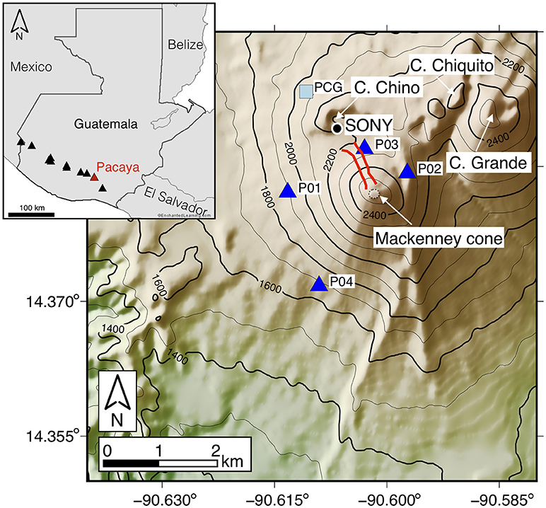
Figure 1. Map of Pacaya volcano showing the location of the seismic stations used in this study (blue triangles). The single permanent station of the local network, PCG, is shown by the light blue square. The black circle indicates the position of the portable SONY video camera used during the field campaign. Red lines indicate the linear depression that developed during the May 27, 2010 eruption. Contour interval is 100 m. The box in the upper left corner shows the position of Pacaya volcano in Guatemala with respect to the Central American Volcanic Arc volcanoes marked as black triangles.
Beginning in January 2013, the volcano entered a new period of increased activity taking place mainly at the Mackenney cone and characterized by more continuous and energetic strombolian eruptions, ash eruptions and lava flows often accompanied by strong seismic tremor as reported by INSIVUMEH (Instituto Nacional de Sismologìa, Vulcanologìa, Meterologìa and Hidrologìa). Tremor was not only recorded by the INSIVUMEH seismic network, but it was also felt by the population of the nearby villages (Gustavo Chigna, pers. comm.). This new unrest prompted the installation of a local network to augment the single permanent station located ~1 km from the Mackenney cone (PCG—Figure 1) with the aim of monitoring and investigating the seismic activity.
This study focuses on modeling the source mechanism of thousands of small LP events associated with weak strombolian explosions at the summit vent of Pacaya volcano. The persistent volcanic activity and the proximity of numerous villages are just two factors that motivate us to better understand the magmatic processes and structure of this very active volcano. Due to the limited number of stations available for the seismic experiment, we employ a recently developed nonlinear moment-tensor inversion approach (Waite and Lanza, 2016; Lanza and Waite, 2018), which adds a more thorough quantitative evaluation of source mechanism reliability. The study of Lanza and Waite (2018) provides a framework for evaluating moment-tensor solutions for a variety of hypothetical seismic networks and seismic source types. The procedure involves a grid search over all possible moment-tensor types and orientations at the best-fit centroid location and the results provide a range of acceptable models that fit the data. The present study is the first to thoroughly investigate the source processes of Pacaya's shallow LP seismicity.
Data Acquisition and Processing
Temporary Seismic Network
We conducted a seismic experiment at Pacaya volcano during October-November 2013 to study the continuous tremor-like signals and the explosions occurring at the summit crater. Three Guralp CMG-ESPC 3-component broadband seismometers (60s corner period) and one Guralp CMG-40T sensor (30s corner period) were installed around the central vent at distances between 0.6 and 1.5 km from the crater (Figure 1).
Two of these stations (P01 and P02) were also outfitted with 3-element, equilateral triangular infrasound arrays, with ~30 m between elements. Data were recorded on Reftek 130 digitizers operating in continuous mode at 125 samples per second and equipped with Global Positioning Systems (GPS) timing. Concerns about vandalism and theft discouraged us from deploying solar panels; therefore, the experiment ran for about 10 days from 31 October through 10 November. The single permanent station (PCG) from the local network operating at the time has an uncalibrated short-period sensor so the data from that station could not be incorporated into the study.
Visual Observations
During the installation of the temporary seismic network, about ~3 h of video recordings using a SONY HD video camera were acquired. Camera clock was calibrated by hand, referencing hand-held GPS units. The recordings show the occurrence of frequent small strombolian explosions and puffing of gas from the cinder /spatter cones inside the summit vent (Mackenney cone, Figure 2A).
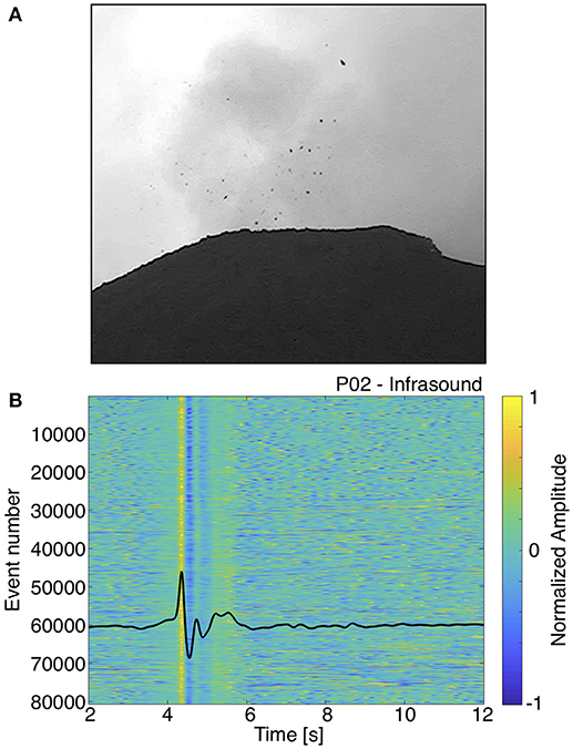
Figure 2. (A) Single frame from a video-recording of one small explosion at the crater recorded on November 3, 2013. The video camera was positioned on Cerro Chino at about 1 km NNW of the Mackenney cone (see black circle in Figure 1). (B) Waveforms of 80,701 events on the infrasonic record over a 10-day long period from 31 October to 11 November 2013, normalized to the maximum absolute amplitude. Plotted in black is the stacked infrasound template event used in the matched filter approach.
LP Events
During the 10 days the temporary network was operative, the infrasound network recorded thousands of impulsive events with an inter-event time of about 1–2 s. Because the events were more clear in the infrasound than the seismic, we used one of these events as a template and performed waveform cross-correlation to search for similar events within the acoustic record. Cross-correlation is carried out on filtered data bandpassed between 0.5 and 10 Hz. By applying this time-domain matched filter approach, we were able to identify hundreds of events that correlated with the template with a cross-correlation coefficient of 0.9 or higher, which were stacked to create a new template (Shearer, 1994; Richardson and Waite, 2013). To improve the signal-to-noise (S/N) ratio of the template, we then ran this new template through the dataset again with a cross-correlation cut off of 0.8. In this way, we identified more than 80,000 events over a 10-day long period from 31 October to 11 November 2013 (Figure 2B). This infrasound catalog was then used to extract the corresponding waveforms from seismic data. This revealed the presence of a repetitive seismic signal (LP event type) associated with the acoustic emissions that was not clearly visible above the background tremor and/or other noise sources (Figure 3). With the term association we here refer to those LP events that are happening at the same time of the infrasound pulses and that have a cross-correlation > 0.8. These amount to 32,908 events in the same 10-day time period.
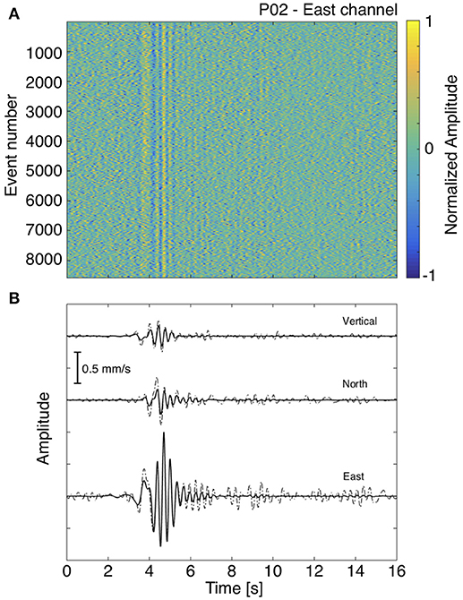
Figure 3. (A) Waveforms of 8,587 seismic events with S/N greater than 1.2 observed on station P02 (east channel) over the same 10-day long period used for the infrasound detections. Waveforms are normalized to the maximum absolute amplitude. (B) Stacked seismograms for all three-components at station P02. Both linear time-domain (dashed lines) and phase-weighted stacks (bold lines) are shown.
While the infrasound data helped to identify the associated seismic event, the seismic data had minor time shifts when aligned with the times of the infrasound events. While the seismic velocity structure was presumably stable over the course of the deployment, variations in wind velocity and air temperature may have produced small variations in the sound speed profile between the vent and our array. In order to overcome this, we cross-correlated one channel of the seismic data at each station to determine time shifts that would improve the alignment. These shifts were on the order of 0.1 s.
We reduced the number of events from 32,908 to 8,587 by considering only those events that have a S/N ratio greater than 1.2 on the east component of station P02 (Figure 3A). We then followed the phase-weighted stacking approach (Schimmel and Paulssen, 1997; Thurber et al., 2014), which resulted in waveforms with an improved signal to noise ratio when compared to the linear stacks. Although the phase-weighted stack is slightly lower in amplitude, the pre- or post-event noise is much lower (Figure 3B).
One additional challenge in obtaining a representative stacked seismic event resulted from the somewhat discontinuous nature of the seismic data. Because the stations were not all contemporaneously operational, simply stacking waveforms to obtain a waveform that would synthesize the response from all four stations would produce a stack with disproportionally low amplitudes for those stations with fewer events. We employed a method described by Richardson and Waite (2013) to assure correct amplitudes in the stacks. As station P02 was running concurrently with all the other stations, we used it to tie events recorded by different stations and to compare amplitudes. Since the east component is consistently the highest amplitude component for P02, we used it as the reference channel. For each of the other stations, we generated temporary stacked seismograms of P02 east that included only the events recorded by the station of interest (i.e., Figures 4A–C, bottom row, panel 1). We then calculated the ratio of the stack for a particular component to that of the P02 east component stack for the same subset of events (Figures 4A–C, bottom row, panel 2). In this way, all the channels were converted from stacked amplitudes to amplitudes proportional to the east component of P02 (Figures 4A–C, bottom row, panel 3). All stacked amplitudes were then converted back to true amplitudes proportional to one of the largest observed LP events seen at P02 through simple multiplication of each trace by the maximum velocity amplitude of P02 for that event.
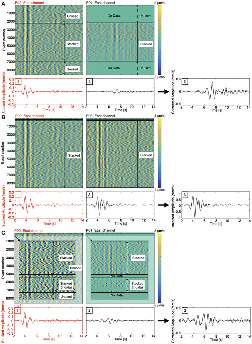
Figure 4. Stacking procedure for east components of P02 and P04 (A), P02 and P03 (B), P02 and P01 (C). P02 is the reference station used for normalization. (A) top row: waveforms of events recorded at P02 and at P04; black lines indicate the stacking interval used for P04. Waveforms are bandpass filtered between 0.5 and 2.0 Hz, and amplitudes are scaled appropriately to the color bar. Bottom row, panel 1: we show in red the phase-weighted (solid line) and linear (dashed line) stacks for P02 over the stacking interval of P04. Bottom row, panel 2: we show in black the phase-weighted (solid line) and linear (dashed line) stacks for P04. In panel 3, we show the phase-weighted and linear stacks of the east component waveform for P04 with amplitude normalized by the maximum absolute amplitude of the P02 stack over the stacking interval station P04. (B) and (C) same as (A) but for stations P03 and P01 respectively.
At the two closest stations, P02 and P03, the main part of the signal lasts 2.5–3 s. The coda, a significant component of which is likely due to scattering, continues for more than 10 s. Interestingly the largest amplitudes at these closest stations, which are ~600 m east and 500 m north of the summit vent, respectively, are on the east component. This is also the case at P01, which lies 1200 m west of the source. While the dominant E-W signal is not so clear on station P04, 1500 m SW of the summit, it is evidence of a significant E-W feature of the source-time process.
We prepared the stacked waveforms for the full-waveform inversion by band-pass filtering 0.5–2 Hz with a zero-phase Butterworth filter. The data were also downsampled from 125 samples per seconds (sps) to 50 sps, trimmed, and multiplied by a cosine tapered window centered on the highest amplitudes. Last, we transformed the data into the frequency domain.
LP Inversion
Full-Waveform Inversion Procedure
We followed an inversion approach that is similar to other studies (see e.g., Auger et al., 2006; Waite et al., 2008; Dawson et al., 2011; Richardson and Waite, 2013) where the inversion is performed in the frequency domain to reduce the computation time and permit a grid search over a large volume. With this approach, we solved for the full spectra of the bandpass filtered (0.5–2 Hz) seismograms and invert at each frequency separately. In terms of the classic least-squares inversion equation, d = Gm, d represents the vector of complex spectra for a single frequency for all the data channels, G represents the matrix of Green's functions for that frequency, and m represents the spectral component of the corresponding source components (e.g., six moment-tensor components). After inverting for each frequency, the source-time functions for the model components are computed from their inverse Fourier transforms.
This procedure is performed at thousands of points within the three-dimensional (3D) model of the volcano, allowing to scan the model space for location. In this paper, the inversion is initially unconstrained, meaning that the inversion is performed for different combinations of the nine free parameters (six moment-tensor components and three single forces) with no constraint on the source-time functions. In some cases, this leads to an unrealistic and uninterpretable set of time histories for the source components, but this is quantified through the similarity of the waveforms. The moment tensor is comprised of force couples, but because mass advection processes can also produce single forces on the Earth, it's important to consider the single forces as parameters to invert for in source inversions of volcanic signals. Examples for which the single forces have been used to explain the seismic signals recorded at volcanoes include Asama volcano, where the results of the waveform analyses of 5 explosion earthquakes indicated that a vertical single force dominated the force system at the source region (Ohminato et al., 2006); lateral ejection of material at Mount St. Helens in 1980 was also attributed to a single force system (Kanamori and Given, 1982), and LPs recorded at Villarica volcano were related to a single force resulting from a bursting bubble in the lava lake and the responsive drag force of the lava sloshing to fill in the void produced by the gas emissions (Richardson and Waite, 2013).
We here adopt the term MT+F to describe unconstrained inversions that include all nine free parameters; the term MT indicates unconstrained inversions that only include six moment-tensor components; and the term F here stands for unconstrained inversions performed using only single forces. In a second step, “constrained” inversions at the best-fit centroid obtained from the unconstrained inversions are performed as part of the nonlinear inversion procedure which involves a grid search over all possible moment-tensor types and orientations.
For both unconstrained and constrained inversions, synthetic Green's functions were computed with the 3D finite-difference method of Ohminato and Chouet (1997). We used a cosine smoothing function to synthetize the Green's functions and assure stability. This wavelet has a time constant period of 1 s (1 Hz) to approximate the peak frequency of the LP events recorded at Pacaya volcano. The Green's functions convolved with the cosine function represent the elementary source-time functions used in the inversion. We used a model that includes the 3D topography of Pacaya, derived from a digital elevation map (DEM) from 2006 with a resolution of 10 m. The model domain is centered on the active summit crater of the volcano (Mackenney cone), and it has lateral dimensions of 4 by 4 km and a vertical extent of 3.5 km. This yields a model with 401 × 401 × 351 nodes spaced 10 m apart. All station locations were rounded to the nearest node, and topography was resampled to match the correct node grid. The node spacing satisfies the criterion of minimum number of grids per wavelength of 25 established through a trial-and-error approach by Ohminato and Chouet (1997) to insure a stable computation. The model is also wide enough to minimize edge reflections of the boundaries while including all the stations. To find the best location for each of the point sources, we conducted a grid search over a volume of 740 × 740 × 500 m centered on the summit vent at a spacing of 20 m. In order to reduce the number of calculations required to derive the Green's functions, we followed Chouet et al. (2005), and used the reciprocal relation (Aki and Richards, 2002) between source and receiver in which each station is treated as a point source and each potential source as a receiver.
Nonlinear Inversion Procedure
As described in Waite and Lanza (2016) and Lanza and Waite (2018) we explore the uncertainty in the source type through a grid search over all possible moment-tensor types and orientations. In this nonlinear inversion, the single forces are kept as free parameters when they are included.
The search over source types is determined using the fundamental lune source-type definition of Tape and Tape (2012). Similar to a Hudson-type plot (Hudson et al., 1989), the lune maps the distribution of all possible moment-tensor source types onto a surface. Source types are defined by two parameters, the spherical coordinates γ and δ, which are defined by the ratios of the moment-tensor eigenvalues. The longitude parameter, γ, ranges from −30° to 30°, and it is defined as:
where L1, L2, and L3 are the eigenvalues of each point of the source-time function.
The latitude parameter, δ, ranges from −90° to 90°, and it is derived from the co-latitude parameter, β, for which:
where L1, L2, and L3 are the eigenvalues of each point of the source-time function. The latitude δ is zero for deviatoric patterns, and both δ and γ are zero for double couple mechanisms.
The search over the γ and δ uses the surface spline method described in Tape and Tape (2012), which effectively reduces the number of points required to evenly sample the distribution over an evenly spaced grid. We evaluate the full range of γ and δ and the full lune are shown for the real data. However, for the synthetic tests, because we didn't use time-shifts, we show only the upper half of the lune which is in this case simply the opposite sign of the lower half (e.g., net positive isotropic versus net negative isotropic).
In addition to exploring the full source-type space, the range of possible orientations for each source is also examined. To do this, we rotate the moment tensor at 10° intervals using a sequence of three rotations about the initial coordinate system of the moment tensor. Complete sampling of the symmetric tensor orientations requires exploring three rotations: a full 360° range about one axis, for example, the z axis; a range from 0 to 180° of dip of z to z'; and finally, 90° of rotation about the new, rotated z' axis (Goldstein et al., 2002; Waite and Lanza, 2016). The 10° interval was chosen for computational reasons after having assessed, through multiple tests with finer intervals, that although there are small changes in the misfit values, there were no significant changes in the pattern of misfits. This involves 5832 combinations of rotation angles combined with 223 γ-δ pairs, for a total of 1,300,536 trial moment-tensor solutions.
For each individual moment source-type in the gridded lune we invert for the source-time function that provides the best fit to the data by fixing the moment tensor and fitting the best source-time function. We refer to Waite and Lanza (2016) for the details of the inversion approach.
Evaluation of the Inversion Results
The overall selection of the best solution was based on a weighted squared error between the observed and modeled data described as E2 (Ohminato et al., 1998; Chouet et al., 2003):
where is the pth sample of the nth data trace, is the pth sample of the nth synthetic trace, Ns is the number of samples in each trace, and Nr is the number of three-component receivers. Here the squared error is normalized by station, so that stations with varying amplitude contribute equally to the error. We adopt E2 error as it accounts for stations from all distances equally; with just four stations we felt it more important to find a well-balanced of fit on all receivers, rather than favoring only the nearest stations with the largest amplitude arrivals. The use of misfit information here is not only employed to define uncertainty on the source centroid as a result of the unconstrained inversions, but also to examine the uncertainty in the moment-tensor type.
For the unconstrained inversion results, the influence of the number of free parameters in each source model was evaluated by calculating the Akaike's information criterion (AIC; Akaike, 1974), expressed as:
where E2 is the squared error from equation (4), Nm is the number of source mechanisms, and Nf is the number of frequencies in the passband of interest. In general, the use of more free parameters is considered justified when both the squared error and AIC are reduced.
Evaluation of the Velocity Model
We considered a homogeneous velocity model with P-wave velocity of 978 m/s, S-wave velocity of 565 m/s and density of 1750 kg/m3. These values are based on the mean of the first 5 layers (first 130 m in depth) of the shear-wave velocity model of Lanza et al. (2016), which was derived from Love and Rayleigh dispersion curves. While this homogenous model is not ideal, we did not have a detailed 3D model available. In order to evaluate how the limitations in the velocity model influence the solution, we performed synthetic tests that use a smooth 1D model. The 1D model follows the topography and is composed of 2 layers followed by a half space. The first layer extends until 100 m depth and we assigned P-velocity of 866 m/s, so that it will be lower than the homogeneous model in which VP is set to 978 m/s. This choice is functional to test the presence of a low velocity layer, which is very common in volcanic areas. The second layer extends until 530 m, which is the maximum depth reached by the S- wave velocity model of Lanza et al. (2016). This layer has a P-velocity of 1.66 km/s obtained by averaging the VP velocities of Lanza et al. (2016)'s model for layers encompassing the same depths. A P-wave velocity of 3.05 km/s was assigned to the half space. The S wave speed is fixed at Vp/√3. For each layer, the density was calculated averaging by depth the density values derived from the model of Lanza et al. (2016), so that the first layer has a density of 1.99 g/cm3, the second layer of 2.24 g/cm3, and the half space of 2.56 g/cm3.
For the synthetic tests, we computed synthetic Green's functions in both homogeneous and 1D models for a vertical crack input model striking 80° E with dipole magnitude ratios of [3, 1, 1] (γ = −30°, δ = 60.5°). Synthetic tests involving different source types (from double couple to isotropic sources) were also carried out in a parallel study that focused on the assessment of network performances for moment-tensor studies of long-period events at volcanoes, in which one of the network array considered mirrored the one deployed at Pacaya volcano (Lanza and Waite, 2018). To synthesize a realistic set of seismograms, the Green's functions calculated for the input source model were convolved with a portion of the Mxx component of the source-time function obtained from the unconstrained inversion of data (see section Inversion Results). Synthetics were computed for (1) an input location situated 260 m directly beneath the highest point in the topographical model of Pacaya volcano, at 2330 m a. s. l. where all source points are below topography in order to minimize possible edge effects in the Green's functions; (2) an input location situated 100 m beneath the crater, in order to consider a case of a very shallow source. Both locations are chosen to be directly beneath the active summit vent based on the initial hypothesis that the close association of seismic and infrasound events, tied by visual observations, is related to a source located below the summit vent. To simulate noisy traces in real data, white noise bandpass filtered in the LP band was added to the final synthetic waveforms. Noise amplitude was calculated using the average of the root mean squared of the synthetic signal amplitudes from the four stations. In this way, the noise amplitude was constant across the network.
We modeled synthetic data through both the homogeneous and the smooth 1D model at the two chosen depths. For all cases, we inverted the synthetic waveforms using the Green's functions generated for the homogeneous velocity model in an effort to simulate modeling real data with Green's functions from a homogeneous model. While inversions of synthetic data computed in the homogenous model were very good, the moment-tensor source-time functions from the 1D model synthetics have a shift in the source type from the initial input crack model toward a linear-vector dipole (LVD) source mechanism, with a much broader γ and δ distribution (Figure 5). The values of E2 are higher with respect to the misfits obtained with the homogenous model. Since the lune plots do not give the orientation of the source, we plotted the eigenvectors of the best fit moment tensors in the top left corners of Figure 5 as rose diagrams of the azimuth ϕ. The original orientation is recovered well in the homogeneous case (Figures 5A,C), while it presents some deviations from the original input orientation for the solution obtained with the 1D smooth velocity model (Figures 5B,D) for both depths considered. These tests confirm an expected degradation of the accuracy of the solution related to the incorrect velocity model (Bean et al., 2008) and shallow depth (Trovato et al., 2016). However, even with an incorrect velocity, which usually constitutes one of the major unknowns in source modeling studies, we can constrain the reconstructed source mechanism to a region of the lune that includes source types similar to the input source model.
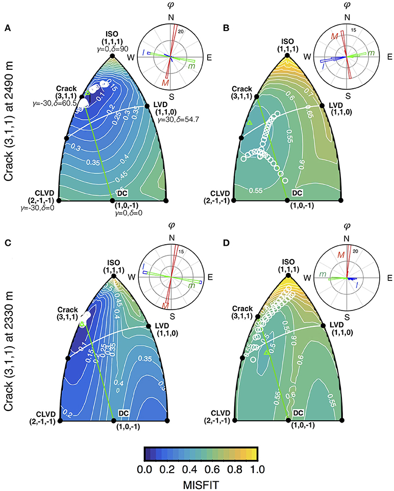
Figure 5. Misfit by fixed moment tensor solution, plotted together with the point-by-point eigenvalue decomposition of the moment-tensor solution for the unconstrained inversion as white circles for a crack input source model located at 2490 m, and 2330 m a.s.l. The green triangles indicate the γ-δ pairs with the minimum misfit. (A) Solution for synthetic data generated with a homogeneous velocity model. (B) Solution for synthetic data generated with a 1D velocity model. (C) and (D) same as (A) and (B) but for an input source located at 2330 m a.s.l. Rose diagrams show the orientations of the maximum, intermediate and minimum eigenvectors for the unconstrained inversion solutions.
Inversion Results
Unconstrained Inversion Results
Data were first inverted in the 0.5–2 Hz band without constraining the solution in any way. We prefer this method for searching over possible source centroid locations. We solved for three types of source models: single forces alone (F); moment-tensor components alone (MT); and a combination of both single forces and moment components (MT+F). We then use several approaches for evaluating the best model from these inversion results as has been done in prior work (e.g., Matoza et al., 2015).
Generally, source locations for all of the unconstrained inversion trials (F, MT, and MT+F) are displaced from the summit; they are either to the north for the F, MT+F and a local minimum of solutions for the MT, or to the east for the global minimum solution for the MT inversion. All reveal a shallow source location ranging from 20 to 240 m below the highest topographical point (Figure 6). Given the close association between the seismic and the infrasound signal associated with these events we are confident that the true LP source is shallow and just below the vent.
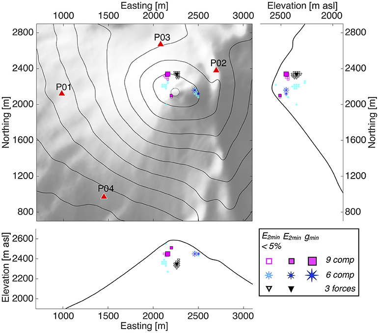
Figure 6. Locations of best-fit source centroids for minimum misfit (E2min), for all solutions within 5% of the minimum misfit (E2min < 5 %), and when both source-time function stability and minimum misfit are considered (gmin). Locations for all three unconstrained inversion trials are shown. Contour interval is 100 m. Red triangles indicate the broadband network position.
The error in centroid location is primarily attributed to the homogeneous model used in the inversion, but the uncertainties seen in the hypocenter location can be a result of a combination of errors in the velocity model and station distribution. And even though the first arrivals are difficult to time accurately, it is clear from the signal travel time move-out that the LP source must be located within the upper cone.
The best-fit model, based on both the residual error estimates and AIC, is the one that includes a combination of six moment-tensor components and three single forces (MT+F), as seen in Table 1. However, the choice of the best source model has to consider not only an assessment of the overall misfits, but also an evaluation of whether the model is geologically reasonable. We explore interpretations of the single forces in terms of other observations of the events and previous work to determine if they are reasonable, or more likely a result of an artifact, such as unmodeled structure in the edifice.
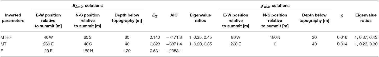
Table 1. Unconstrained inversion results.
Because no constraints on the source type were used in these inversions, the model source-time function components can be inconsistent over time, resulting in a difficult to interpret, geologically unreasonable model. For source nodes having E2 within 5% of the minimum, we calculated the consistency of the source-time function over its duration using the standard deviations of the ratios of the eigenvalues. This measurement is expressed by a statistic called gamma by Matoza et al. (2015), and g by Waite and Lanza (2016) to avoid possible confusion with the previously defined moment-tensor lune longitude. The parameter g is obtained by calculating the square root of the sum of the squared standard deviations of the ratios of the minimum to maximum and intermediate to maximum eigenvalues for each time in the source history (also equation 6 in Matoza et al., 2015):
where σ is the standard deviation, and α1, α2, α3 are the minimum, intermediate, and maximum moment-tensor eigenvalues, respectively. The standard deviations provide a measure of the consistency of the source-time function over its duration, so we seek a solution that both minimized the misfit (low E2) and has a consistent set of moment-tensor components (low g).
We computed the ratio of eigenvalues at each point in the source-time function having amplitude greater than 60% of the maximum to reduce the influence of noise in low-amplitudes. For both the MT and MT+F models, the solution with the lowest value of g within these error volumes is very similar to the source-time function at the minimum E2, both in terms of the misfit and the moment tensor. The best-fit source centroids for minimum misfit, together with the gmin best-fit locations, and all the solutions within 5% of the minimum misfit, are shown in Figure 6.
We note that although the absolute value of g is a function of the moment-tensor eigenvalue ratios assumed in the calculation, this assumption does not significantly influence the identification of the solution with the lowest value for g. For example, Waite and Lanza (2016), based on a priori information, used moment-tensor eigenvalue ratios of 2:1:1 for examining g values for a source-time function of a VLP signal recorded at Fuego volcano. They also considered different ratios and found that although the values for g vary, there was no difference in which solutions had the lowest g. Based on those results, we simply assumed ratios of 1:1:1 in our computations for g. We computed a similar statistic for the case of single forces only which is based only on the consistency of the single-force source-time functions, but we do not report this here to avoid unnecessary complexity when comparing to the moment components. In summary, for the MT and MT+F models, both solutions with minimum E2 and those with minimum g have moment-tensor source-time functions that are consistent throughout the time history of the source.
Based on the model fits (E2 = 0.531), and the AIC (AIC = −2353.1), we first discard the force-only solution. In addition to fact that it has the worst fit, which is partially due to the smaller number of parameters used in the inversion, the single forces only inversion source-time function components are not in phase, indicating that the mechanism is not stable in time (see Figure S2). The largest force is in the east-west direction, which is consistent with the large east-west component on the nearest stations. But the overall poor fit to the data suggests this is not a reasonable model for this stacked event (Figure S1).
We next consider the subtle differences between the MT and the MT+F solutions. Both have a moment tensor somewhat like a dipping crack with similar solutions for both the minimum E2min and minimum gmin solutions. The E2min misfits are 0.323 and 0.140 for MT and MT+F, respectively (Table 1). The model synthetic fits to the data are quite good and match the large amplitudes on the east components much better than the single force model does. For brevity, we focus on results from the E2min MT model, but include results from the MT+F inversions and the gmin MT model in the supplementary materials (Figures S3–S6). For reasons described below, we favor the model that does not include single forces. Figure 7 shows the data (black) along with the modeled waveforms for the MT E2min solutions. The unconstrained inversion synthetics, shown in red, generally fit the data fairly well. The synthetics from the fixed tensor solution, shown in cyan and described in the following section, have greater misfits, as expected for models with fewer free parameters. A similar plot for the MT+F model is shown in Figure S3.
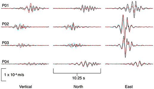
Figure 7. Waveform fits for the representative LP event obtained from the phase-weighted stacks of 8,587 repeating events. Fits are for the E2min solution for the 6- components unconstrained inversion. Red lines indicate unconstrained -inversion synthetics, cyan lines are best-fitting constrained inversion synthetics, and black lines represent observed velocity waveforms.
The source-time functions for both the unconstrained and constrained MT inversion are shown in Figure 8A. We used the general formulation convention with Mxx oriented East, Myy North, and Mzz Up. Note how the dipole components Mxx and Mzz are in phase, even for the unconstrained inversions, and dominate the source-time function.
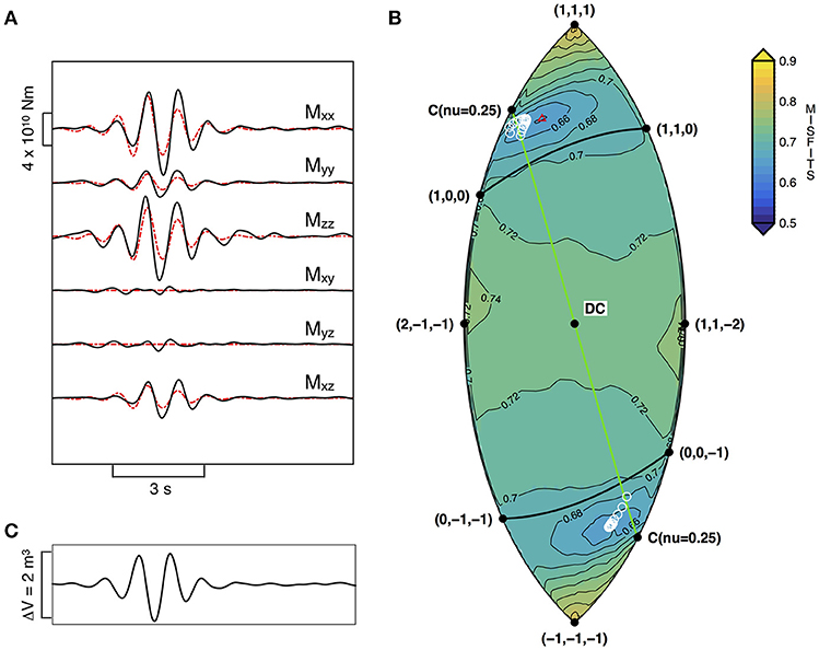
Figure 8. (A) Source-time function from the MT unconstrained inversion (black line), and for the E2min solution from the constrained inversion (dashed red line). (B) Misfit by fixed moment-tensor solution, plotted together with the γ-δ distribution for the unconstrained inversion (white circles), and with the γ-δ pair for the constrained inversion (red triangle). (C) Estimated volume change for the source-time function of the MT solution.
The source-time function of the unconstrained MT inversion is further analyzed through point-by-point eigenvector decomposition. We use only points with amplitude of at least 60% of the peak amplitude to assure stability. Figure 9 shows the statistics of the eigenvectors through rose diagrams of the azimuth ϕ, and inclination angle ϑ, measured from the vertical. For each point of the source-time history, we calculated the longitude γ and the latitude δ of the fundamental lune and the ratios of minimum and intermediate eigenvalues to the largest, whose median values are reported in Table 1. The eigenvector analysis and the point-by-point γ-δ pairs define a fairly constrained solution in the region that includes sources from a tension crack (white circles in Figure 8B) dipping ~40° to the east (ϕ = −6.4°).
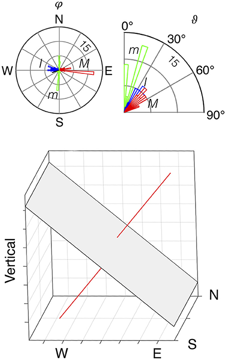
Figure 9. Eigenvector statistic for the unconstrained MT inversion solution. The smallest (m), intermediate (I), and largest (M) eigenvectors are shown by green, blue, and red bins, respectively. ϕ is the azimuth, measured clockwise from north and ϑ is the inclination angle, measured from the vertical. The orientation of the crack plane and its normal (maximum eigenvector) are also shown in the xyz coordinate system.
Although the network includes only four stations, they are well distributed. The solution behaves consistently through time, in agreement with the finding by Lanza and Waite (2018) that the azimuthal coverage has an important influence in the stability of the source-time function compared to factors such as the number of stations used in the inversion.
Constrained Inversion Results
The source-time functions derived from the unconstrained inversion were further investigated through constrained inversions for source type. Again, we focus on results for the MT inversion, but include results from the MT+F inversions in the supplementary materials. Figure 8B shows the misfits at each moment-tensor type for the lowest misfit tensor orientation. That is, each point in the lune plot represents the lowest misfit value for all moment-tensor orientations with the particular γ - δ pair. The misfits for the constrained inversion results are much larger than those of the unconstrained inversions, ranging from values of 0.64 to 0.84, with respect to the minimum value of 0.32 obtained from the unconstrained inversion. This is not unexpected given that there is essentially one model parameter in the constrained inversions, compared to six independent model parameters for the unconstrained inversions. The nonlinear inversion suggests a slightly larger area of possible source mechanisms types; however the region surrounding 5% above the minimum occupies an area in which all the eigenvalues are the same sign. Uncertainties of the moment tensor for each component and cross-components trade-off in the moment tensors within this area are explored by calculating the ratios of each moment components with the moment components of the best fitting solution (red triangle in Figure 8B). As shown in Figure S7, the cross-components Mxy and Myz components are poorly constrained compared to the other components which, instead, show a tighter range of variation.
The ratio of eigenvalues (0.20, 0.42, 1) from the nonlinear inversion points to a source not precisely like a known theoretical source. It is somewhat like a theoretical tensile crack in a Poisson solid (1, 1, 3) in which the largest eigenvalue is perpendicular to the crack, but with less symmetry in the in-plane deformation. This is explored further below.
The constrained inversions for the MT+F inversions (Figures S4, S5) have much lower misfit values but appear to be completely unconstrained. While the best-fit mechanisms are very close to the mechanisms determined from the unconstrained inversions for MT+F, the area of acceptably low misfit covers most of the lune. We attribute this result to the lack of constraint on the single forces. For nearly any mechanism type, the combination of the three unconstrained single force model parameters and one moment tensor model parameter can fit the data reasonably well. So, in this model, the use of the full lune is not as illustrative of model fit.
Discussion
The LP events we recorded at Pacaya volcano in 2013 are associated with small explosive outgassing events at the summit. With a scalar seismic moment of about 4x10¹⁰ Nm, these events release about as much energy as a Mw 1 earthquake. The fact that this same source was activated as often as every 1–2 s, with larger, clearer signals about every 15 s during our short deployment, suggests this dominant style of activity is important to understand. We rely on the infrasound record of these events, along with our visual observations of puffing and weak explosions, to inform our interpretation of the seismic moment tensor and help constrain the models. Given the association of the seismic LP with the infrasound source we attribute the LPs to strombolian bubble-burst events. Here we interpret the seismic source models to provide some constraints on the process involved in these explosions and on the conduit structure just below the vent.
The ascent of a bubble, and the flow of magma down and around it should produce a reaction force in the Earth. Assuming a nearly vertical conduit, we should expect to see a nearly vertical single force together with a moment tensor that models some associated conduit deformation. This has been seen in laboratory experiments (James et al., 2009) and in data from other volcanoes. One excellent example is the Kilauea VLP source model of Chouet et al. (2010). They modeled VLP events as resulting from the ascent, expansion, and burst of a large slug of gas. They interpreted the presence of a dominant vertical single force as a result of an upward force on the Earth induced by the approaching of the slug to the surface and consequent pressure decrease and conduit deflation below the slug. The magnitudes of the vertical forces were consistent with slug masses of 104 to 106 kg.
In another study involving a bubble ascent mechanism, Richardson and Waite (2013) found that a dipping single force model provided the best-fit to repetitive LPs associated with strombolian explosions at Villarrica volcano. In that case, the E-W oriented particle motions at all azimuths were attributed to near horizontal viscous forces associated with a structural feature in the upper conduit. The moment-tensor components were not required by the data.
In the case of Pacaya, the single forces involved in the source process might be too small to model. We estimate the mass of bubbles that produce the small strombolian explosions we observe as LP events assuming a monopole source in which the mass emission as a function of time, q(t), can be estimated as (Lighthill, 1978; Firstov and Kravchenko, 1996):
where r is distance from the source, c is the speed of sound (~340 m/s) and p represents the excess pressure time series. This approach was extended by Johnson and Miller (2014) to ensure zero net pressure over a finite window around the recorded event. We then calculated the mass of gas from discrete infrasound events using the integral of mass emission rate. These events, which have amplitudes between 1 and 3 Pa at our closest sensors, are up to about 500 kg. These values are similar to those Dalton et al. (2010) estimated from records of Pacaya in 2008), a time period in which the style of summit activity was very similar to the 2013 activity. They found repeated events characteristic of strombolian explosions with peak amplitudes ranging from 0.17 to 2.61 Pa at about twice the distance of our array in 2013 (~1 km) and estimated masses of 12 to 962 kg.
The vertical single forces in the MT+F inversions have amplitudes on the order of 5-10 x109 N. When we compare the amplitudes of the modeled single forces to prior work on bubble ascent, we find they are orders of magnitude too large. Using the empirical scaling relation of James et al. (2009), in which the magnitude of the upward force is proportional to the square root of the slug mass, and the magnitude of our vertical single force of nearly 1.0 GN, we estimated a slug mass of up to 108 kg. Even considering the uncertainties associated with our mass estimates, we should not expect to be five orders of magnitude in error.
Any single force associated with the ascent of these bubbles must be many orders of magnitude smaller than what we find with our MT+F inversion. The inversion results, therefore might be unreliable due to the small number of stations (12 channels) we model. In a study of synthetic sources, Lanza and Waite (2018) found that there is a strong trade-off between single forces and moment tensor components when they are in phase. Further they found that inverting for single forces can increase the discrepancy between the modeled and input moment tensors. A similar study by Trovato et al. (2016) also points to challenges with MT+F inversions. While the source process we model here may involve mass advection or another process that would lead to a single force, the actual forces are likely much too small to be reliably modeled.
We therefore attribute the most reasonable data fit to a 6-component (MT) mechanism. The best-fitting source for the MT inversion when both source-time function stability and minimum misfit are considered is found ~200 m to the ESE of the summit of the Mackenney cone at 2450 m above sea level, corresponding to about 40 m below the highest node in the topographical model in this location (Figure 6). While the model epicenter is displaced from the active vent, the shallow depth is consistent with the related infrasound and observed explosions and the epicentral error is likely a result of inaccuracies in the velocity model.
An important challenge of this work is that we are working with a small number of stations. We can clearly identify a dominant LP event but questioned how reliably we could resolve the source mechanism. Synthetic tests described in Lanza and Waite (2018) have shown that a complete azimuthal coverage, with a maximum gap of about 130°, is desired for a higher resolution of the retrieved source-time function. They also stated that azimuthal coverage has a larger influence on network performances over the number of stations used. However, for sources with a large isotropic component, four stations were deemed to be the limit of acceptable performances as with a lower number of stations the source mechanisms are unconstrained. Therefore, the case study of Pacaya where LP events were recorded by a network of only four stations with a fairly good azimuthal coverage should provide a reasonable model of the source mechanism.
As shown by additional synthetic tests described in this study, an unknown velocity model can introduce a further degradation of the solution. Although the source-time function is constrained to a region in which sources have a large isotropic component, the range of source-type shown in Figure 8 could reflect the effect of a scarcity of stations and of an incorrect velocity model.
With that in mind, we find that both the constrained and unconstrained inversions point to a source mechanism somewhat like a tension crack but with less symmetry. The nonlinear inversions indicate a range of possible solutions could fit the data reasonably well. The magnitude of the derived moment tensor is around 4 x 10¹⁰ Nm. This is comparable to moment-tensor solutions obtained for low-amplitude LPs at other volcanoes. At Mount St. Helens, Matoza et al. (2015) inverted small LP events and found a moment tensor with amplitudes on the order of 1010 Nm. Small LP events have been also imaged at Popocatepetl, Mexico, and showed moment-tensor components of similar order of magnitude (Arciniega-Ceballos et al., 2012). In both cases the low-amplitude LP events were related to shallow crack mechanisms and interpreted as hydrothermally driven fractures. At Pacaya, while the source mechanism is not precisely a theoretical crack, we can interpret it as a source that is dominated by volume change, consistent with a repetitive source that is associated with bubble bursts. We estimate the volume change in the source-time function from the amplitude (λ +2μ)ΔV, assuming ν = 1/4 (λ = μ) as the source-time function occupies a region along the arc with ν = 1/4 in the fundamental lune (Figure 8C). We use a shear modulus for the crack wall rock of 10 GPa following Lyons and Waite's (2011) study at Fuego volcano. The calculated volume change is ~ 2 m3. This value reflects the representative average event obtained from the stacked waveforms, and it is reasonable for the size of the events recorded. We used the relationship between excess pressure and volume change in a penny-shaped crack (equation 11 from Chouet et al., 2010) to estimate the crack width as ~2.3 m. We envision the crack not as an isolated feature, but as a component of the shallow conduit that responds to the passage of these bubbles.
A schematic of the proposed physical interpretation of the source of these small shallow long-period events is shown in Figure 10. As gas slugs rise toward the surface, they expand and burst, creating an initial positive infrasonic pulse followed by a negative pulse. This generates the infrasound signal which was also observed in 2008 by Dalton et al. (2010). Both LPs and the acoustic waves show compressional first motions, with LP signals preceding the infrasound by ~ 1 s. The time delay is compatible with a source that simultaneously causes both the seismic and infrasound, given an airwave travel time of nearly 2 s and seismic travel time of under a second. One possibility is that the LPs are a manifestation of the reaction force to the expansion and ejection of the slugs (or bubbles). While the coupling of this source could possibly explain the dipping crack-like moment tensor, a simple calculation of the vertical force associated with bubble expansion (Gerst et al., 2013) indicates that it is perhaps 6 orders of magnitude smaller than would be required to explain the seismic moment of the LP.
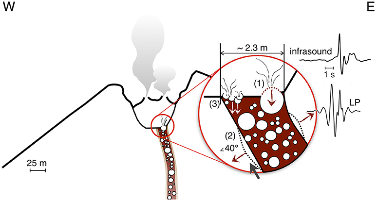
Figure 10. Schematic of the proposed interpretations of the source-time function of the small long-period events recorded at Pacaya: (1) LPs seen as a manifestation of the reaction force to the expansion and ejection of the bubbles; (2) LPs seen as originating from the movement of the bubbles through an inclined crack that inflates and deflates as a result of the passage of fluids; (3) LPs seen as the results of bubbles that act as a volumetric source exploding at the surface with a sudden release in pressure.
A second explanation is that the non-destructive LP events originate from the movement of the slugs (or bubbles) through a N-S oriented, dipping crack that inflates and deflates as a result of the passage of fluids; when the slugs (bubbles) reach the lava free surface, they burst creating the infrasound signals. Given the short delay between the seismic and infrasound arrivals, the LP crack source must be very close to the surface, but this mechanism is compatible with timing of infrasound and seismic arrivals and the observations of E-W particle motions at stations west, north, and east of the summit.
Another possible explanation to the source dominated by isotropic components obtained by our inversion could involve the presence of bubbles that act as a volumetric source exploding at the surface with the sudden release in pressure. Distortions in the wavefield caused by propagation through the near-vertical walls of the conduit could explain why the mechanism is not calculated as perfectly isotropic.
In the broader context of the Mackenney cone and the recent eruptive history, the N-S orientation of the seismic source is consistent with both shallow and somewhat deeper features. The NNW oriented depression that developed during the 2010 eruption, shares a similar orientation. Flank vents, both north and south of the summit vent, have formed since the 2010 eruption. Modeling of InSAR data collected in from 2012-2014 points to the repeated opening of a NNW oriented dike within the upper 400 m of Mackenney cone (Wnuk and Wauthier, 2017). The Mackenney cone itself is built upon the scarp of a prehistoric flank collapse to the WSW and recent largescale motion of that flank has been in roughly the same direction (Schaefer et al., 2017). The conduit just below the vent, as modeled by the shallow LP seismicity, shares this dominant N-S direction imparted by deeper structures.
Concluding Remarks
We investigated the source mechanism and geometry of a class of LP events that includes thousands of small, repetitive, events that are associated with weak strombolian explosions at the summit vent of Pacaya volcano, Guatemala. LP events were recorded in October-November 2013 by four broadband stations located around the summit. Tremor-like seismic signals dominate the records at Pacaya during much of the deployment, but we find that the tremor is comprised in part by many small events, closely spaced in time. By employing the less noisy infrasound records to identify discrete events, we generate a representative LP event that we model with full waveform inversion.
Uncertainty in the velocity model and the small number of stations employed in the inversion allow for a certain degree of ambiguity in the source location, but we can clearly demonstrate that this event involves volume change in the source process. Our modeling demonstrates that the LP events reflect a shallow crack-like mechanism most likely related to bubble-bursting events at the summit. The N-S orientation of the model crack is consistent with aligned surficial features including vents and the NNW oriented depression that formed during the May 2010 explosive eruption. Similarly, dikes modeled geodetically have a N-S orientation such that the conduit must be elongated N-S throughout the edifice. Our study of 10 days of seismic data represents only a snapshot of the dynamic recent history of Pacaya volcano, but the combined seismic-infrasound approach provides constraints on the magmatic processes within the shallow conduit and the relationship between conduit structure and the overall structure of the Mackenney cone.
Data Availability
Data collected during the 2013 experiment are available through the IRIS Data Management Center. The facilities of the IRIS Consortium are supported by the National Science Foundation under Cooperative Agreement EAR-0552316 and by the Department of Energy National Nuclear Security Administration. The phase-weighted stacking code was provided by D. Mikesell.
Author Contributions
FL took part in the seismic network installation, performed initial data processing for the temporary array, carried out the full waveform moment-tensor inversion, and wrote the first draft of the manuscript. GPW supervised all the work, advised FL on data processing, contributed to the development of the nonlinear inversion methodology, and provided revisions for/edited the manuscript. All authors read and approved the submitted manuscript.
Funding
This work has been supported by the National Science Foundation Career Award No. 1053794 entitled Eruption Dynamics From Low-Frequency Volcano-Seismic Signals.
Conflict of Interest Statement
The authors declare that the research was conducted in the absence of any commercial or financial relationships that could be construed as a potential conflict of interest.
Acknowledgments
We thank J. Richardson for his guidance and fieldwork support. We are grateful to Parque Nacional Volcán de Pacaya and INSIVUMEH for allowing access and permission to install seismometers. We also thank two reviewers and Chief Editor Valerio Acocella for their useful comments which resulted in this improved version of the original manuscript.
Supplementary Material
The Supplementary Material for this article can be found online at: https://www.frontiersin.org/articles/10.3389/feart.2018.00139/full#supplementary-material
References
Akaike, H. (1974). A new look at the statistical model identification. IEEE Trans. Automat. Control 19, 716–723. doi: 10.1109/TAC.1974.1100705
Aki, K., and Richards, P. G. (2002). Quantitative seismology, 2nd Edn. Sausalito, CA: University Science Books.
Arciniega-Ceballos, A., Dawson, P. B., and Chouet, B. A. (2012). Long period seismic source characterization at Popocatépetl volcano, Mexico, Geophys. Res. Lett. 39:L20307. doi: 10.1029/2012GL053494
Auger, E., D'Auria, L., Martini, M., Chouet, B. A., and Dawson, P. B. (2006). Real-time monitoring and massive inversion of source parameters of very long period seismic signals: An application to Stromboli Volcano, Italy. Geophys. Res. Lett. 33:L04301. doi: 10.1029/2005GL024703
Bean, C. J., Lokmer, I., and O'Brien, G. S. (2008). Influence of near-surface volcanic structure on long-period seismic signals and on moment tensor inversions: Simulated examples from Mount Etna. J. Geophys. Res. 113:B08308. doi: 10.1029/2007JB005468
Chouet, B. A. (1996). “New methods and future trends in seismological volcano monitoring,” in Monitoring and Mitigation of Volcano Hazards, eds R. Scarpa and R. I. Tilling (New York, NY: Springer-Verlag), 23–97.
Chouet, B. A., Dawson, P. B., and Arciniega-Ceballos, A. (2005). Source mechanism of Vulcanian degassing at Popocatepetl Volcano, Mexico, determined from waveform inversions of very long period signal. J. Geophys. Res. 110:B07301. doi: 10.1029/2004JB003524
Chouet, B. A., Dawson, P. B., James, M. R., and Lane, S. J. (2010). Seismic source mechanism of degassing bursts at Kilauea Volcano, Hawaii: results from waveform inversion in the 10–50 s band. J. Geophys. Res. 115:B09311. doi: 10.1029/2009JB006661
Chouet, B. A., Dawson, P. B., Ohminato, T., Martini, M., Saccorotti, G., Giudicepietro, F., et al. (2003). Source mechanisms of explosions at Stromboli Volcano, Italy, determined from moment-tensor inversion of very-long-period data. J. Geophys. Res. 108:2019. doi: 10.1029/2003JB002535
Chouet, B. A., and Matoza, R. S. (2013). A multi-decadal view of seismic methods for detecting precursors of magma movement and eruption. J. Volcanol. Geotherm. Res. 252, 108–175. doi: 10.1016/j.jvolgeores.2012.11.013
Dalton, M. P., Waite, G. P., Watson, I. M., and Nadeau, P. A. (2010). Multiparameter quantification of gas release during weak Strombolian eruptions at Pacaya volcano, Guatemala. Geophys. Res. Lett. 37:L09303. doi: 10.1029/2010GL042617
Dawson, P. B., Chouet, B. A., and Power, J. (2011). Determining the seismic source mechanism and location for an explosive eruption with limited observational data: Augustine Volcano, Alaska. Geophys. Res. Lett. 38:L03302. doi: 10.1029/2010GL045977
Firstov, P. P., and Kravchenko, N. M. (1996). Estimation of the amount of explosive gas released in volcanic eruptions using air waves. Volcanol. Seismol. 17, 547–560.
Gerst, A., Hort, M., Aster, R. C., Johnson, J. B., and Kyle, P. R. (2013). The first second of volcanic eruptions from the Erebus volcano lava lake, Antarctica—Energies, pressures, seismology, and infrasound. J. Geophys. Res. Solid Earth 118, 3318–3340. doi: 10.1002/jgrb.50234
Goldstein, H., Poole, C. P., and Safko, J. L. (2002). Classical Mechanics, 3rd Edn. San Francisco: Addison Wesley. doi: 10.1119/1.1484149
Hudson, J. A., Pearce, R. G., and Rogers, R. M. (1989). Source type plot for inversion of the moment tensor. J. Geophys. Res. 94, 765–774.
James, M. R., Lane, S. J., Wilson, L., and Corder, S. B. (2009). Degassing at low magma-viscosity volcanoes: Quantifying the transition between passive bubble-burst and Strombolian eruption. J. Volcanol. Geotherm. Res. 180, 81–88. doi: 10.1016/j.jvolgeores.2008.09.002
Johnson, J. B., and Miller, A. J. C. (2014). Application of the monopole source to quantify explosive flux during vulcanian explosions at sakurajima volcano (Japan). Seismol. Res. Lett. 85, 1163–1176. doi: 10.1785/0220140058
Kanamori, H., and Given, J. W. (1982). Analysis of long-period seismic waves excited by the May 18, 1980, eruption of mount St. Helens – A Terrestrial Monopole? J. Geophys. Res. 87, 5422–5432.
Kitamura, S., and Matías, O. (1995). Tephra stratigraphic approach to the eruptive history of Pacaya volcano, Guatemala. Sci. Rep. Tohoku Univ. Seventh Ser. 45, 1–41.
Lanza, F., Kenyon, L. M., and Waite, G. P. (2016). Near-surface velocity structure of Pacaya volcano, Guatemala, derived from small-aperture array analysis of seismic tremor. Bull. Seism. Soc. Am. 106, 1438–1445. doi: 10.1785/0120150275
Lanza, F., and Waite, G. P. (2018). A nonlinear approach to assess network performance for moment-tensor studies of long-period signals in volcanic settings. Geophys. J. Int. 215, 1352–1367. doi: 10.1093/gji/ggy338
Lyons, J. J., and Waite, G. P. (2011). Dynamics of explosive volcanism at Fuego volcano imaged with very long period seismicity. J. Geophys. Res. 116:B09303. doi: 10.1029/2011JB008521
Matoza, R. S., Chouet, B. A., Dawson, P. B., Shearer, P. M., Haney, M. M., Waite, G. P., et al. (2015). Source mechanism of small long-period events at Mount St. Helens in July 2005 using template matching, phase-weighted stacking, and full-waveform inversion. J. Geophys. Res. 120, 6351–6364. doi: 10.1002/2015jb012279
Ohminato, T., Chouet, B. A. (1997). A free-surface boundary condition for including 3D topography in the finite-difference method. Bull. Seism. Soc. Am. 87, 494–515.
Ohminato, T., Chouet, B. A., Dawson, P. B., and Kedar, S. (1998). Waveform inversion of very long period impulsive signals associated with magmatic injection beneath Kilauea Volcano. J. Geophys. Res. 103, 839–823. doi: 10.1029/98JB01122
Ohminato, T., Takeo, M., Kumagai, H., Yamashina, T., Oikawa, J., Koyama, E., et al. (2006). Vulcanian eruptions with dominant single force components observed during the Asama 2004 volcanic activity in Japan. Earth Planets Space. 58, 583–593. doi: 10.1186/BF03351955
Richardson, J. P., and Waite, G. P. (2013). Waveform inversion of shallow repetitive long period events at Villarrica Volcano, Chile. J. Geophys. Res. 118, 4922–4936. doi: 10.1002/jgrb.50354
Rose, W. I., Palma, J. L., Escobar Wolf, R., and Matias, O. (2013). “A 50 yr eruption of a basaltic composite cone: Pacaya, Guatemala,” in Understanding Open-Vent Volcanism and Related Hazards, eds W. I. Rose, J. L. Palma, H. D. Granados, and N. Varley (Boulder, CO: Geological Society of America).
Schaefer, L. N., Wang, T., Escobar-Wolf, R., Oommen, T., Lu, Z., Kim, J., et al. (2017). Three-dimensional displacements of a large volcano flank movement during the May 2010 eruptions at Pacaya Volcano, Guatemala. Geophys. Res. Lett. 44, 135–142. doi: 10.1002/2016GL071402
Schimmel, M., and Paulssen, H. (1997). Noise reduction and detection of weak, coherent signals through phase-weighted stacks. Geophys. J. Int. 130, 497–505. doi: 10.1111/j.1365-246X.1997.tb05664.x
Shearer, P. M. (1994). Global seismic event detection using a matched filter on long-period seismograms. J. Geophys Res. 99, 13713–13725. doi: 10.1029/94JB00498
Tape, W., and Tape, C. (2012). A geometric setting for moment tensors. Geophys. J. Int. 190, 476–498. doi: 10.1111/j.1365-246X.2012.05491.x
Thurber, C. H., Zeng, X., Thomas, A. M., and Audet, P. (2014). Phase-weighted stacking applied to low-frequency earthquakes. Bull. Seism. Soc. Am. 104, 2567–2572. doi: 10.1785/0120140077
Trovato, C., Lokmer, I., De Martin, F., and Aochi, H. (2016). Long period (LP) events on Mt Etna volcano (Italy): the influence of velocity structures on moment tensor inversion. Geophys. J. Int. 207, 785–810. doi: 10.1093/gji/ggw285
Waite, G. P., Chouet, B. A., and Dawson, P. B. (2008). Eruption dynamics at Mount St. Helens imaged from broadband seismic waveforms: Interaction of the shallow magmatic and hydrothermal systems. J. Geophys. Res. 113:B02305. doi: 10.1029/2007JB005259
Waite, G. P., and Lanza, F. (2016). Nonlinear inversion of tilt-affected very-long-period records 1 of explosive eruptions at Fuego volcano. J. Geophys. Res. 121, 7284–7297. doi: 10.1002/2016JB013287
Keywords: long-period event, phase-weighted stacking, waveform inversion, source processes, Pacaya volcano
Citation: Lanza F and Waite GP (2018) Nonlinear Moment-Tensor Inversion of Repetitive Long-Periods Events Recorded at Pacaya Volcano, Guatemala. Front. Earth Sci. 6:139. doi: 10.3389/feart.2018.00139
Received: 13 June 2018; Accepted: 04 September 2018;
Published: 25 September 2018.
Edited by:
Benoit Taisne, Nanyang Technological University, SingaporeReviewed by:
Yosuke Aoki, The University of Tokyo, JapanCynthia J. Ebinger, Tulane University, United States
Copyright © 2018 Lanza and Waite. This is an open-access article distributed under the terms of the Creative Commons Attribution License (CC BY). The use, distribution or reproduction in other forums is permitted, provided the original author(s) and the copyright owner(s) are credited and that the original publication in this journal is cited, in accordance with accepted academic practice. No use, distribution or reproduction is permitted which does not comply with these terms.
*Correspondence: Federica Lanza, ZmxhbnphQHdpc2MuZWR1